| Issue |
A&A
Volume 661, May 2022
|
|
|---|---|---|
| Article Number | A138 | |
| Number of page(s) | 18 | |
| Section | Galactic structure, stellar clusters and populations | |
| DOI | https://doi.org/10.1051/0004-6361/202142667 | |
| Published online | 19 May 2022 | |
Prospects of measuring a metallicity trend and spread in globular clusters from low-resolution spectroscopy⋆
1
Leibniz-Institut für Astrophysik Potsdam (AIP), An der Sternwarte 16, 14482 Potsdam, Germany
e-mail: This email address is being protected from spambots. You need JavaScript enabled to view it.
2
Indian Institute of Astrophysics, Koramangala II Block, Bangalore 560034, India
3
Pondicherry University, R.V. Nagar, Kalapet, 605014 Puducherry, India
4
NAT – Universidade Cidade de São Paulo/Universidade Cruzeiro do Sul, Rua Galvão Bueno 868, São Paulo-SP 01506-000, Brazil
5
CRAL-Observatoire de Lyon, Université de Lyon, Lyon I, CNRS, UMR5574, St-Genis-Laval, France
Received:
15
November
2021
Accepted:
17
February
2022
Abstract
Context. The metallicity spread, or the metallicity trend along the evolutionary sequence of a globular cluster, is a rich source of information to help understand the cluster physics (e.g., multiple populations) and stellar physics (e.g., atomic diffusion). Low-resolution integral-field-unit spectroscopy in the optical with the MUSE spectrograph is an attractive prospect if it can provide these diagnostics because it allows us to efficiently extract spectra of a large fraction of the cluster stars with only a few telescope pointings.
Aims. We investigate the possibilities of full-spectrum fitting to derive stellar parameters and chemical abundances at low spectral resolution (R ∼ 2000).
Methods. We reanalysed 1584 MUSE spectra of 1061 stars above the turn-off of NGC 6397 using FERRE and employing two different synthetic libraries.
Results. We derive the equivalent iron abundance [Fe/H]e for fixed values of [α/Fe] (solar or enhanced). We find that (i) the interpolation schema and grid mesh are not critical for the precision, metallicity spread, and trend; (ii) with the two considered grids, [Fe/H]e increases by ∼0.2 dex along the sub-giant branch, starting from the turn-off of the main sequence; (iii) restricting the wavelength range to the optical decreases the precision significantly; and (iv) the precision obtained with the synthetic libraries is lower than the precision obtained previously with empirical libraries.
Conclusions. Full-spectrum fitting provides reproducible results that are robust to the choice of the reference grid of synthetic spectra and to the details of the analysis. The [Fe/H]e increase along the sub-giant branch is in stark contrast with the nearly constant iron abundance previously found with empirical libraries. The precision of the measurements (0.05 dex on [Fe/H]e) is currently not sufficient to assess the intrinsic chemical abundance spreads, but this may change with deeper observations. Improvements of the synthetic spectra are still needed to deliver the full possibilities of full-spectrum fitting.
Key words: methods: data analysis / techniques: spectroscopic / stars: abundances / stars: fundamental parameters / globular clusters: individual: NGC 6397
The table with the results for each individual star is only available in electronic format the CDS via anonymous ftp to cdsarc.u-strasbg.fr (130.79.128.5) or via http://cdsarc.u-strasbg.fr/viz-bin/cat/J/A+A/661/A138
© ESO 2022
1. Introduction
Globular clusters (GCs) are studied for their own sakes, for instance, to investigate the characteristics of their stellar population and infer their formation and evolution processes. They are also benchmarks for probing theories of stellar physics, such as the variations in the surface chemical composition of stars with respect to their initial composition as expected from atomic diffusion (Chapman 1917).
Significant abundance spreads were documented in Gratton et al. (2012) or Mészáros et al. (2015), for example, with amplitudes larger by more than 0.1 dex for the α-elements. With a few exceptions such as ω Cen and Terzan 5, the iron ([Fe/H]) spreads are in contrast lower than the observational uncertainties in general (about 0.05 dex; Carretta et al. 2009). Some abundance trends (i.e. systematic change along the temperature sequence of the cluster) were also suggested (Korn et al. 2007; Lind et al. 2008; Nordlander et al. 2012, in NGC 6397). These studies are at the precision limit of the measurements, and a number of observational or modelling effects can mislead the interpretation.
In these investigations, the authors analysed observations with high signal-to-noise ratio (S/N) and high spectral resolution of as many stars as possible. However, these observations are expensive because the multiplexing capability of high-resolution spectrographs is limited and exposure times are long, and they are hampered by crowding in the central regions of the clusters. The final samples are therefore often restricted to typically a dozen stars in the outskirts of the cluster. Low-resolution integral-field-unit (IFU) spectroscopy may be considered as an alternative. It benefits from a large multiplexing and from the development of crowded-field spectroscopy (Kamann et al. 2013).
The MUSE IFU spectrograph, attached to the ESO Very Large Telescope (Bacon et al. 2010), allows observing a significant fraction of a Galactic GC in a single telescope pointing. It has been used by Husser et al. (2016, hereafter H16) to observe NGC 6397, where the parameters of about 1600 stars above the turn-off (TO) point of the main sequence were measured. Because of the low spectral resolution (R ∼ 2000), individual spectral lines from different chemical species are blended, and classical methods are not applicable. Therefore, the authors used full-spectrum fitting (see e.g., Koleva et al. 2009), where all the spectral bins are compared at once to reference spectra to derive the atmospheric parameters such as effective temperature (Teff), surface gravity (log g), and [Fe/H]. This has demonstrated that low-resolution IFU spectroscopy can be effective at analysing large samples of stars in a GC with good internal precision. H16 found a [Fe/H] trend of ∼0.2 dex along the effective temperature sequence, but when the same dataset was reanalysed by Jain et al. (2020, hereafter J20), the iron abundance was found to be nearly constant ([Fe/H] ∼ −2.0 dex). Both studies used the full-spectrum fitting technique to derive the parameters, and the origins of the different results lie in the details of the analyses. Specifically, while H16 was using synthetic spectra from the Göttingen Spectral Library1 (hereafter GSL; Husser et al. 2013) as reference, J20 used empirical libraries (ELODIE; Prugniel & Soubiran 2001; Wu et al. 2011, and MILES; Sánchez-Blázquez et al. 2006). We also stress that with full-spectrum fitting, the derived iron abundance depends on the abundance pattern inscribed in the set of reference spectra. For this reason, we call it an equivalent iron abundance, hereafter noted [Fe/H]e, whose relation to the true abundance has to be considered with care.
To assess the external accuracy of these results, we need to understand the systematics caused by the analysis methods, such as those due to the interpolation performed within the spectral library and those due to the adopted libraries. Comparing the results obtained with different libraries and methods may give a lower limit of this second source of errors.
As a step in this direction, we reanalyse here the set of MUSE observations previously used by H16 and J20. We use a different analysis tool and different sets of reference models to explore the prospects of using full-spectrum fitting methods to derive accurate parameters from the analysis of low-resolution stellar spectra. The paper is organised as follows: in Sect. 2 we present the observational material, and in Sect. 3 we describe the analysis method based on FERRE2 (Allende-Prieto 2015). Section 4 presents the analysis with the GSL grid (the same grid as was used by H16), hence allowing us to compare the results and investigate the effect of the interpolation scheme and of other details of the setup. In Sect. 5 we carry out the analysis with the Allende Prieto et al. (2018, hereafter AP18) grid of models to investigate the effect of the choice of model and of the mesh size. We finally discuss the different aspects that affect the ability of measuring metallicity trends and spreads in Sect. 6, and we draw conclusions in Sect. 7.
2. Observational material
NGC 6397 was observed during the MUSE commissioning between July 26 and August 3, 2014 (ESO ID program 60.A-9100(C)). The observations consist of a 5 × 5 square mosaic (two tiles are missing) and reach about 3.5 arcmin from the cluster centre on its diagonal. They are based on 127 pointings with exposure times of about 60 s to avoid saturation of the brightest stars for a total integration time of 95 min. Each pointing covers a field of 1 × 1 arcmin, and the seeing is between 0.6 and 1 arcsec. All the data have already been reduced by the MUSE consortium using the official pipeline. The MUSE spectra cover a wide wavelength range, λλ = 470 − 950 nm, with a resolution R = λ/Δλ ∼ 2000, where λ is the wavelength, and Δλ the full width at half maximum (FWHM) of an unresolved line.
The spectra were extracted by H16 (see that paper for further details) and were downloaded from the website set for commissioning data3. The typical S/N of stars at the TO is ∼50 on average, and the brightest giants reach S/N ∼ 200. The table with photometry and measurements made in H16 were kindly provided by Tim-Oliver Husser (priv. comm.). We corrected the spectra for the telluric absorption by dividing each stellar spectrum by the corresponding telluric spectrum determined by H16. We then reduced the spectra to the rest-frame velocity by changing the world coordinate system (WCS), using the mean velocity of the cluster. Because the sampling is not exactly the same in all the spectra (starting wavelength at 4749.75 or 4750 Å), we rebinned all of them to the same WCS to simplify the analysis with FERRE (see Sect. 3). The normalisation of the spectra to their continuum was performed during the analysis in order to employ the same algorithm and parameters for the observations and the models. The weight of the individual spectral bins was computed assuming a constant S/N throughout the spectrum. We experimented with various weighting schemes and retained the scheme that provided the best precision.
These commissioning observations are based on short observing time and moderate image quality (they were obtained before the ground-layer adaptive optics entered routine use to improve the image quality). Moreover, since that early epoch, the data reduction software has been improved. Still, this public collection of reduced spectra is unique in its the possibility of comparing different approaches for measuring stellar atmospheric parameters.
2.1. Selected sample and surface gravities
H16 used this observational material to determine the atmospheric parameters of 4132 stars from 5881 spectra (because the individual tiles of the mosaic overlap, some stars were observed more than once) with S/N > 20. With this S/N cut-off, the formal errors on Teff and [Fe/H]e are lower than 100 K and 0.16 dex for stars along the giant and sub-giant (SG) branches, and near the TO, as discussed by H16. Later, J20 restricted this sample further to the cluster members (based on the radial velocity), excluded the hot stars (restricting to Teff < 7000 K), and finally selected only the stars with log g < 4.2. This resulted in a sample of 1587 spectra for 1063 stars.
We adopt the values of log g computed by H16 using the photometry from Anderson et al. (2008) and isochrones from Bressan et al. (2012). J20 has shown that fitting log g at the same time as Teff and [Fe/H]e produces results consistent with the photometric log g and does not affect the observed iron abundance trend. Adopting this photometric log g simplifies the comparison with the earlier studies.
In the J20 sample, three of the 1587 stars have log g < 1, but the two model grids that we use (GSL and AP18) start at log g = 1 because the slice at log g = 0 is incomplete (see Sect. 4 for further details). Thus, we excluded them from our analysis, and the final sample consists of 1584 spectra for 1061 stars.
2.2. Injection of the line-spread function
The full-spectrum fitting method we used involves comparing each spectral bin of an observed spectrum to the corresponding bin of model spectra and searching for the physical parameters that provide the best match (in a χ2 sense). Because models are computed at a high resolution, they must be transformed to have the same line-spread function (LSF) as the observations. This process is called LSF injection, and the function used in the transformation is called relative LSF.
The mean LSF of the MUSE spectra varies with wavelength, and it varies by 0.1 Å across the 24 spectrographs that form MUSE. H16 has pointed out the difficulty of accurately matching the LSF for each individual spectrum, and following them and J20, we neglected the variation between the different spectrograph. This simplification is justified a posteriori in Sect. 4.3 by testing the effect of the LSF width and centring on the uncertainties.
To model its variation across the wavelength range, we defined the LSF in two segments, and we used a piece-wise convolution similar to the implementation in ULySS4 (Koleva et al. 2009). As the GSL and AP18 models have the same spectral resolution (R = 10 000), we adopted the same relative Gaussian LSF for both: at λ = 4750 Å, the FWHM is 2.75 Å, at λ = 7000 Å, it is 2.45 Å, and at λ = 9300 Å, it is 2.50 Å. Moreover, we noticed a small shift in the NIR range, for which the spectra were corrected by adding a 0.20 Å shift at λ = 9300 Å. Each model spectrum was convolved with these three LSFs, and the final model was obtained by interpolating linearly in wavelength between the first and second spectra for wavelengths smaller than 7000 Å, and between the second and third spectra for larger wavelengths.
3. Analysis code: FERRE
In H16 and J20, similar codes were used in the analysis, namely spexxy5 and ULySS, respectively. The main difference is in the adopted models: while H16 used the GSL synthetic library, J20, employed empirical spectra. We used FERRE, a public code for full-spectrum fitting, notably used in the SEGUE stellar parameter pipeline (Lee et al. 2008) and in the APOGEE pipeline (García Pérez et al. 2016, ASPCAP). Briefly, it interpolates between the nodes of an evenly sampled grid of synthetic stellar models and performs a χ2 minimisation to find the parameters of the model that best reproduce the observed spectrum. We used two different model grids: GSL and AP18 (described in Sects. 4 and 5).
FERRE offers a choice of optimisation algorithms (we used the default Nelder-Mead minimisation algorithm6), of different interpolation schemes in the grid, and of different normalisations of the spectra to their pseudo-continuum. Thus, it allows us to investigate how the different algorithms of interpolation in the grids could affect the measurements.
In spexxy or ULySS, the broadening function and systemic velocity are fitted at the same time as the atmospheric parameters, as well as a multiplicative polynomial that absorbs the differences in flux calibration between the observation and the reference spectra. Fitting these parameters simultaneously with the atmospheric parameters avoids biases that may occur when the different parameters are partially degenerate, but it requires more computations. In contrast, FERRE does not adjust the broadening and continuum: the observations and the model grid should have the same LSF and be normalised in the same way. These are the essential differences between the two approaches.
3.1. Equivalent iron abundance
While classical abundance methods at high spectral resolution (R ∼ 40 000) measure individual resolved lines, full-spectrum fitting uses the complete spectral information by combining all the spectral lines from any chemical species present in the considered wavelength range. This is an optimal use of the signal, and thus opens the method to the exploitation of low S/N spectra (e.g., in SEGUE, [Fe/H] was determined for spectra with S/N > 10 by Lee et al. 2008), and of low- and medium-resolution spectra.
A rigorous application of this method would be to simultaneously determine the abundances of all the elements that significantly contribute to the opacity in the considered wavelength range. This would be very difficult for two reasons. Firstly, because the larger the number of free parameters, the more unstable the fit. Secondly, because this will require a grid with separate dimensions sampling each chemical element. This is not practically feasible because of the excessively large volume of data it would represent, and because of the time needed to compute such a grid. The usual simplification is to fit only one or two abundance parameters, typically [Fe/H] or [Fe/H] plus [α/Fe], and assume a fixed (solar) pattern for the other elements: for this reason, we refer to the metallicity as the equivalent iron abundance ([Fe/H]e). A mismatch between the assumed and real pattern will result in biases of the derived parameters. For example, if a spectrum enhanced in α-elements is fit with solar-scaled reference spectra, the measured equivalent [Fe/H]e would be larger than the true one: the iron lines will be over-fitted, and the α-elements will be under-fitted. A strategy for measuring the abundance of individual α-elements has been tried at higher spectral resolution in the ASPCAP pipeline (García Pérez et al. 2016). It consists of determining [Fe/H] and [α/Fe] first, and then using spectral masks to isolate the lines of each element to measure its abundance. This approach is probably difficult to use at the MUSE resolution, where the lines are blended.
In the following analysis, we use a fixed abundance pattern, either with [α/Fe] = 0, or with enhanced α-elements ([α/Fe] = 0.4 or 0.5 dex) corresponding to the pattern expected in NGC 6397. The first equivalent [Fe/H]e is expected to over-estimate the real iron abundance, and the second is expected to be a more accurate estimate.
3.2. Interpolation schemes
As already mentioned in the previous section, FERRE has different options for interpolating the models at any arbitrary location in the parameter space, namely, linear interpolation, and quadratic and cubic Beziér splines following the description in Auer (2003). These methods are local interpolations, computed on two (for linear) to four (for cubic interpolations) neighbours on each axis7.
Although all the interpolation schemes implemented in FERRE are locally infinitely derivable over their computation interval, the overall interpolating function is continuous but not derivable at the nodes. On each side of a node, a different interpolation neighbourhood is used, and the local interpolating functions are therefore different. In contrast, a true spline interpolation, like in Press et al. (1992), would be derivable at the nodes, but it would be more demanding in computation time and memory storage.
Mészáros & Allende Prieto (2013) evaluated the accuracy of the different interpolation schemes. They computed synthetic models at random locations in the parameter space between the nodes of the grids and compared them to those derived by interpolating the grid. They found that the cubic interpolation schemes produce residuals that are about 40% smaller than the linear interpolation, and are marginally better than the quadratic interpolation. We therefore adopted the cubic Beziér spline interpolation as a default choice (i.e. we use this method when not specified otherwise), and we used the other methods to perform comparisons.
3.3. Normalisation to the pseudo-continuum
The observations and the models were normalised in the same way before the minimisation was run. This is essential to avoid that a mismatch in the shape of the continuum does not contribute to the χ2, which would unavoidably happen even with the most carefully flux-calibrated spectra (because of uncertainties in the flux calibration or in the correction for Galactic extinction). This normalisation was made using a running average implemented in FERRE. The code also has two other normalisation methods that we did not find appropriate for the present work: polynomial, which is limited to very low degrees, and segmented average, which does not remove the local shape of the spectral energy distribution.
3.4. Default set-up
Unless otherwise indicated, we adopted the following setup. We run FERRE on the complete MUSE wavelength range, λλ = 4749.52 − 9300 Å. The effect of using different wavelength ranges is discussed in Sect. 6. We adopted the cubic interpolation, because this option was preferred by Mészáros & Allende Prieto (2013) and it indeed produces satisfactory results. We evaluate the importance of this choice in Sect. 4.4. As normalisation scheme, we chose the running mean with a default window of 60 pixels (i.e. 75 Å), as with this value the residuals (i.e. the difference between the observed and fitted spectra) appear flat. We evaluate the sensitivity of this parameter in Sect. 4.5. As initial guesses for the stellar parameters, we set Teff = 5500 K and [Fe/H] = −1.9 dex. We tested that other choices, such as starting from the photometric Teff or from Teff = 4500 K, do not affect the solutions. As in H16 and J20, we kept log g fixed to the photometric value (see Sect. 2.1). We fixed [α/Fe] = 0.4 dex (for GSL) or 0.5 dex (for AP), as it corresponds to the abundance pattern expected in the cluster. We explore the effect of using [α/Fe] = 0 in Sect. 5.1.
4. Analysis with the GSL grid
GSL is a grid of high-resolution synthetic spectra created with the PHOENIX stellar atmosphere code (Hauschildt & Baron 1999). The spectra were computed in spherical geometry (important in the low-gravity regime) and in local thermal equilibrium (LTE). The structure of the models is similar to the structure of MARCS models (Gustafsson et al. 2008), and they were computed adopting the PHOENIX-ACES equation of state and opacities. The adopted line list comes from Kurucz (2009). GSL covers a wide range of parameters: 2300 < Teff < 12 000 K8, 0 < log g < 6, −4 < [Fe/H] < 1 dex, and −0.2 < [α/Fe]< 1.2 dex.
In GSL, as extensively described in Husser et al. (2013), the micro-turbulence velocity parameter, ξ, is computed from the macro-turbulence velocity, that is, from the convection, and it varies from one model to the other. Its values are stored in the header of the fits files. Abundance ratios are calculated with respect to the solar reference abundances given by Asplund et al. (2009).
We used the version post-processed to a reduced spectral resolution, R = 10 000, over the wavelength range from 3000 to 25 000 Å. We selected grids with fixed [α/Fe] = 0 and +0.4 dex (the latter being a reasonable assumption for low-metallicity GCs), and we restricted the range of the other parameters to what is suitable for the cluster. At low gravity, log g = 0 and 0.5 dex, the temperature coverage of GSL is restricted. For instance, at [Fe/H] = −2 dex, for log g = 0 dex, the coverage is 2300 < Teff < 6000 K. The absence of hotter models is an obstacle for making a grid, because FERRE requires a strictly rectangular grid. We therefore chose to truncate the sample to log g > 1.
4.1. Construction of the grids and analysis
In Fig. 8 of H16, we noticed an irregular distribution of the measurements along the Teff sequence. We investigate these issues in Appendix A and find a non-physical discontinuity at Teff = 5000 K. For this reason, we limited the range of our grid to Teff ≥ 5100 K. The characteristics of the resulting grid are presented in Table 1. FERRE requires the grid to sample each axis evenly9, but the GSL [Fe/H] sampling is not uniform. We show in Fig. 1 (left panel) the parameter space coverage of the grids (the top and bottom rows show the log g versus Teff and [Fe/H] versus Teff planes, respectively), we added the missing [Fe/H] = −2.5 dex slice to GSL by averaging the −2.0 and −3.0 dex slices (red dots in Fig. 1). In Appendix A, we also found an outlier near the TO, and we replaced it with the average between the spectra 100 K apart in the grid. This outlier was found to affect the measurements, while the two others detected in this region were not found to have an impact.
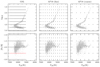 |
Fig. 1. Parameter space coverage of the grids. The grey dots represent the analysed sample, and the black dots mark the nodes of the grids of synthetic spectra. The top panels are the projections on the log g vs. Teff plane, and the bottom panels show the projections in [Fe/H] vs. Teff. The left column is for the GSL (the [Fe/H] = −2.5 dex slice, which is not originally a part of GSL, and is produced by averaging the [Fe/H] = −3 dex and [Fe/H] = −2 dex slices, see Sect. 4). The central column is the AP18 grid (see Sect. 5). The right column is also from the AP18 grid, but with twice larger steps on each axis to evaluate the effect of a coarser grid (see Sect. 5.2). |
Parameter space of the grids.
The procedure of building the grid in the FERRE format has three steps. (i) Conversion from vacuum into air wavelengths, (ii) injection of the relative LSF as described in Sect. 2, and (iii) rebinning as the observations.
When the grid was ready, we ran FERRE. Figure 2 (left column) presents the typical fit of a stellar spectrum. It shows three remarkable regions: around Hβ (spectral window 4790–4940 Å), Mgb (spectral window 5000–5300 Å), and the Ca II triplet (spectral window 8400–8750 Å). The rms of the residuals for the full wavelength range (not shown in the plot) is 0.01. The test spectrum has an estimated S/N of 115, and the residuals indicate a normalised χ2 of 1.7. The figure shows that the LSF and the wavelength calibration are adequately matched, but it also shows significant residuals on strong lines. As already noted in literature, strong lines such as the H lines or the Ca II triplet are difficult to model for a number of reasons, for instance the LTE approximation (see e.g., Martins & Coelho 2007).
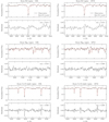 |
Fig. 2. Typical fits of a spectrum (ID = id000010747jd2456866p4985f000). The fit, performed over the complete wavelength range, 4750–9300 Å, returned Teff = 5471 K and [Fe/H]e = −1.84 dex for global rms residuals of 0.01 for both GSL and AP18. The left column shows the [α/Fe] = 0.4 dex GSL grid, and the right column presents the [α/Fe] = 0.5 dex fine AP18 grid. The top row shows a small wavelength region around the Hβ line, the middle row shows a region around the Mgb triplet, and the bottom one shows a region around the Ca II triplet. For each plot, the top panel presents the observation (black line) with the best-fit model over-plotted in red. The bottom panel presents the residuals, observation minus model. |
Table 2 reports the results obtained for the different setups we used. Our measurements of Teff and [Fe/H]e for the individual stars for each combination of wavelength, interpolation, and assumed [α/Fe] are available in electronic form at the CDS. In order to assess the precision and to compare these solutions, we estimated (i) the measurement errors and (ii) the iron abundance spread of the sequence. The measurement errors (due to the noise in the observations, the data reduction, and the analysis) can be reliably estimated using pairs of repeated observations. As in J20, given two observations (1 and 2) of the same star i, we computed  , where Pi is any of the stellar parameters ([Fe/H]e or Teff), and the measurement error ϵ(Pi) is estimated as the rms of ΔPi. Because the iron abundance may change along the sequence of the cluster, the [Fe/H]e dispersion measured over the entire sample would combine the effects of the trend and of the spread. To isolate the spread, we divided the Teff range into bins of 250 K and computed the [Fe/H]e dispersion, σj([Fe/H]), in each bin. For consistency, the final errors and spread, ϵ(Teff), ϵ([Fe/H]) and σ([Fe/H]), are the quadratic average of the ϵj(Pi) and σj(Pi) (Cols. 6–8), and the mean [Fe/H]e (Col. 5) is the average of the mean [Fe/H]e in each bin. As expected, we note that ϵ([Fe/H]) is always smaller than σ([Fe/H]). This reflects the fact that in addition to the effect of the noise and observation, σ([Fe/H]) includes other sources of errors (e.g., due to the precision of the spectral models) and a possible cosmic spread. Finally, the equivalent iron abundance trend τ([Fe/H]) (Col. 9) is defined as the difference between the mean [Fe/H]e in the first and last bins.
Mean iron abundance, errors, dispersion, and trend obtained from different setups, compared with H16 and J20.
4.2. Comparison with H16
Figure 3 compares our measurements with those of H16, both obtained with [α/Fe] = 0. On the left, we compare our Teff (y-axis) and Teff from H16 (x-axis) in the top panel, and at the bottom, we report the difference between our Teff and H16 (ΔTeff(our-H16)) as a function of the Teff from H16. On the right, we show the same set of plots for the [Fe/H]e measurements. Our average equivalent iron abundance is higher by 0.30 dex than the one reported in H16. The rms [Fe/H]e dispersion between the two series is 0.08 dex, which is consistent with the measurement errors. In contrast, there is no overall bias in Teff: the mean difference is −29 K with an rms of 41 K, but there is a significant drift with a ∼100 K amplitude; our values are cooler than those of H16 at the TO.
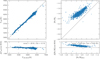 |
Fig. 3. Comparison between our measurements (y-axis) and H16 results (x-axis) obtained with solar [α/Fe]. Bottom panels: differences Δ (our − H16). We report the comparison between the Teff on the left and the comparison between our [Fe/H]e and [Fe/H] of H16 on the right. The mean and rms differences are indicated. |
The two analyses use the same data, the same reference synthetic spectra, and the same technique (full-spectrum fitting). The source of the [Fe/H]e bias and of the temperature drift was searched for in the several differences between the two approaches. The differences due to the analysis programs are that (i) we derived only the atmospheric parameters, while H16 also adjusted the broadening and shift of the spectra, (ii) we used various schema implemented in FERRE to interpolate over the grid of models, while H16 used a cubic spline interpolation, and (iii) we normalised the observed and model spectra to their pseudo-continuum before fitting them, while H16 fitted a multiplicative polynomial at the same time as all the other parameters.
The significance of these three aspects is investigated in detail in the next sections: apparently, they cannot explain the difference of [Fe/H]e between the two analyses. After excluding differences in the programs as a source for the bias, a possible explanation could be searched for in the weighting schema of each individual wavelength bin. To support this hypothesis, we note that the H16 solution is intermediate between our solutions with the full and trimmed to 740 nm wavelength ranges. By decreasing the weight of the near-IR (NIR) region, we can indeed recover a mean [Fe/H]e consistent with H16, but with larger errors. When we use a constant weight throughout the wavelength range, the Teff drift with respect to H16 is cancelled (but the abundance difference remains). We cannot attempt to precisely reproduce the H16 results because we lack information about the weighting that was used. This sensitivity to the weighting reflects inconsistencies in the modelling in different spectral regions, reminiscent of those emphasised by Lançon et al. (2021).
4.3. Effect of the LSF matching
An accurate LSF injection is a priori more critical here than in H16 and J20, where the velocity broadening adjusted to each individual spectrum was absorbing part of its variation throughout the MUSE sample. We carried out two tests to evaluate the effect of the LSF on the parameters. The first test simulated the variation in resolution amongst the MUSE spectrographs, and the second test simulated wavelength shifts that could result from errors in the dispersion relation, or in the rest-frame reduction.
For the first test, we used a GSL grid with an LSF FWHM increased by 0.1 Å, equivalent to the real uncertainty. We find that the Teff increases by 3 K, and [Fe/H]e by 0.01 dex for the whole sample. This is about 10–20% of the measurement errors, and therefore a minor contribution to the error budget.
For the second test, we shifted the LSF by 0.5 Å (i.e. 0.4 times the wavelength bin). This corresponds to about 30 km s−1, that is, about five times higher than the velocity dispersion measured by H16. Here, we find an increase in Teff by 21 K and a decrease in [Fe/H]e by 0.03 dex. Therefore, the wavelength calibration uncertainty and internal velocity dispersion are also minor contributions to the total error.
We note that this second test also mimics the effect of inaccurate line lists that manifests as spectral lines modelled at incorrect wavelengths, or with incorrect strengths. This well-known problem is probably responsible for a significant fraction of the spectral mismatch between observation and models (Franchini et al. 2018; Martins et al. 2019). By splitting the sample into two temperature regimes, we find that [Fe/H]e decreases by 0.04 dex for the warm stars (Teff > 5800 K), while it decreases by only 0.01 dex for the cool stars. This suggests that inaccurate line lists may affect the measured equivalent [Fe/H]e trend.
4.4. Effect of the interpolation schema
The possible importance of interpolation has been pointed out by J20, who noted that the iron abundance trend along the SG branch is only a small fraction of the mesh size. This trend is presented in Fig. 4, in which we compare the H16 measurements with those obtained with FERRE using various interpolation schemes, namely, linear (second panel), quadratic Beziér spline (third panel), and cubic Beziér spline (fourth panel). It is evident that the trend is similar with the different interpolation schemas. The measurement errors (ϵ([Fe/H]) and ϵ(Teff)), the mean and spread of equivalent iron abundance, ⟨[Fe/H]⟩ and σ([Fe/H]) obtained in each case are comparable (see Table 2). This implies that the choice of the interpolation scheme is not critical in this analysis.
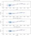 |
Fig. 4. [Fe/H]e vs. Teff diagrams published in H16 (top panel, with [α/Fe] = 0) and those obtained with FERRE using GSL and the three different interpolation schemes (other panels, with [α/Fe] = +0.4). The measurements of individual spectra are shown as blue dots, and the nodes of the grids are overlaid as thin crosses. The red dots and line are the mean [Fe/H]e in bins of 250 K, and the error bars are the dispersion in these bins. |
A peculiar pattern in Fig. 4 is to be mentioned: there is a concentration of measurements aligned on [Fe/H]e = −2.0 dex with the linear, and to a lesser extent with the quadratic interpolation. This is an artefact of the interpolation that is discussed in Appendix B.
4.5. Effect of the continuum normalisation
The observations and the models were both normalised by dividing them by a running mean with a window of 60 wavelength bins, which corresponds to 75 Å. With this width, the residuals of the fits (Fig. 2) do not show low frequencies. We also tested different normalisation windows by fixing the width to twice larger (120) and twice smaller (30). In Table 3 we report the dispersion values corresponding to these tests. The trend is similar in the three cases, and the smaller dispersions obtained with 60 bins justify our choice.
[Fe/H]e dispersion: Effect of the normalisation window.
5. Analysis with AP18 grid
Allende Prieto et al. (2018) provided a comprehensive set of synthetic spectral grids obtained with ATLAS9 atmosphere models, computed by Mészáros et al. (2012) using opacity distribution functions assuming plane-parallel and LTE approximations. The spectra were synthesised with the radiative code ASSϵET (Koesterke 2009). The line lists are from the Kurucz public database (updated in 2007), plus some specific updates. The grids cover the parameter space from 3500 to 30 000 K, 0 to 5 dex, and −5.0 to 0.5 dex for Teff, log g, and [Fe/H], respectively, and also sample [α/Fe] and ξ. The adopted solar reference abundance is from Asplund et al. (2009), as for the GSL grid. Different grids are provided at various spectral resolutions and with various coverage and sampling of this wide domain of parameters.
We used their so-called fine grids ns1 and ns2, at the resolution R = 10 000 (see Table 1 from Allende Prieto et al. 2018), with both solar and enhanced [α/Fe] (+0.50 dex), and with ξ = 1 and 2 km s−1. From our fine grid (AP18 in Table 2), we extracted a coarse grid (APC in Table 2) with a twice larger mesh size. Details can be found in Table 1 and in Fig. 1.
To build our final AP18 and APC grids, we processed them as done for the GSL grid, that is, with the same procedure of LSF injection and rebinning. The only difference was that the AP18 grids were already in air wavelengths.
5.1. Comparison with our GSL results
We repeated the fits of the previous section with the AP18 fine-grained grid with [α/Fe] = 0.5 dex and ξ = 1 km s−1 for the three interpolation schemes. A typical fit is presented in Fig. 2 and can be compared with the fit of the same spectrum with GSL made in Sect. 4. A quantitative comparison of spectral fits with GSL and AP18 grids is made by measuring the mean rms residuals over the whole sample in different spectral regions. We find that these values in the Hβ, Mgb, and Ca II triplet regions are almost the same with both grids. In the full wavelength range (not shown in the plot), as seen with the GSL grid, the rms residual is equal to 0.01.
A comparison of the solutions with AP18 and GSL grids and cubic interpolation is presented in Fig. 5. A systematic difference of equivalent [Fe/H]e is expected because the two grids are computed at different α-elements enhancements, 0.5 dex for AP18, and 0.4 dex for GSL (see Sect. 3.1). The solutions with solar-scaled and enhanced grids are reported in Table 2. For solar-scaled models, when the full wavelength range is considered, the equivalent [Fe/H]e are increased by 0.233 and 0.379 dex for GSL and AP18, respectively. This important effect shows that the α-elements are a major contribution to the total opacity in the considered spectral region. By extrapolating this effect linearly, we can correct the solutions obtained with the two grids to a mid-point enhancement of 0.45 dex. For GSL, the correction is −0.029 dex, and for AP18, it is 0.047 dex. Hence, the mean difference is Δ[Fe/H]e(AP18 − GSL) = − 0.076 dex. This is represented in the figure (dashed blue line), and it closely matches the observed bias of −0.073 dex.
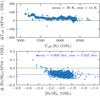 |
Fig. 5. Comparison between Teff and [Fe/H]e obtained with GSL and AP18 grids. Top panel: difference between Teff (ΔTeff(AP18-GSL), computed by subtracting the GSL results from the AP18 results) as a function of Teff values with GSL. Bottom panel: difference of equivalent iron abundance (Δ[Fe/H]e) as a function of the iron abundance with GSL. The dashed blue line shows the expected bias due to the different level of α-element enhancement in the two grids (0.4 vs. 0.5 dex, see the text for details). In both panels we report the mean and rms of the differences. |
The mean biases (AP18 − GSL, reported in the figure) are well within the generally accepted external errors. The rms dispersions between the two series are two to three times smaller than the uncertainties inferred from pair-wise comparisons. This indicates that in our dataset, the random errors linked to the choice of synthetic grid contribute marginally to the error budget.
The [Fe/H]e distributions along the Teff sequence using either linear or cubic interpolation are represented in Fig. 6 (top and central panels). The equivalent iron abundance trend is qualitatively similar to the trend obtained before with GSL: this is also corroborated by the values of τ([Fe/H]) reported in Table 2. As with GSL, the choice of the interpolation scheme does not affect the trend.
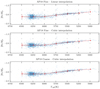 |
Fig. 6. [Fe/H]e vs. Teff relation using the AP18 fine (top and second panels) and coarse (third panel) grids. The top panel shows the linear interpolation, and the two other panels show the cubic interpolation. The grey lines and symbols represent the solution (with an offset of −0.076) obtained with the GSL grid (cubic interpolation) and reported on Fig. 4. The other symbols and line styles are as in Fig. 4. |
Table 2 also shows that the estimated errors (ϵ) and the spreads (σ) are slightly smaller with AP18 than with GSL (by roughly 0.01–0.02 dex). This is consistent with Franchini et al. (2018), who also compared GSL and other grids of synthetic spectra to high-resolution spectra (R ∼ 50 000) obtained in the Gaia-ESO survey (Gilmore et al. 2012) over a 500 Å spectral range around 5200 Å. They found that GSL matches the spectra less well than other libraries.
5.2. Effects of different mesh sizes
A valuable characteristic of the AP18 grid is its fine [Fe/H] sampling. To test the importance of the mesh size, we used the coarse grid (see Table 1), whose [Fe/H] sampling is the same as that of H16. The [Fe/H]e mean value and spread for the coarse grid with different interpolation schema are given in Table 2, and the [Fe/H]e versus Teff diagram with cubic interpolation is shown in Fig. 6 (bottom panel). The values of ϵ([Fe/H]) with the coarse grid are not significantly higher than those with the fine grid, and the mean iron abundance is not affected when quadratic or cubic interpolation is used. With linear interpolation, the dispersion is marginally increased and the mean iron abundance is marginally decreased. We conclude that the mesh size is not critical, and that a 0.5 dex iron abundance step does not affect the results dramatically even for effects ten times smaller than the mesh. Together with the minor effect of changing the interpolation schema seen in Sect. 4.4, this shows that (i) a linear approximation within the considered grids of models is usually satisfactory, and (ii) using a higher-order interpolation schema with a grid mesh as large as 0.5 dex in [Fe/H] allows us to recover the precision of a twice finer mesh.
5.3. Effects of micro-turbulence velocity
Micro-turbulence velocity (ξ) is an ad hoc parameter introduced to account for the difference between the measured and expected strength of spectral lines. The ξ parameter works as an additional broadening and can be derived spectroscopically by imposing that weak and strong iron lines match with the same abundance (see Mucciarelli 2011 for an extensive discussion). It also depends on the other atmospheric parameters: ξ increases with Teff, and it has a tight correlation with log g, being larger in giants than in dwarf stars (Gray et al. 2001; Takeda et al. 2008).
In the series of models used by Lind et al. (2008) to analyse NGC 6397 spectra, ξ decreases from 1.86 ± 0.13 km s−1 at 6250 K (TO) to 1.47 ± 0.09 km s−1 at 5450 K (SG). In the APOGEE ASPCAP analysis (García Pérez et al. 2016), ξ was fixed to a value bound to log g through the relation ξ = 2.478 − 0.325 log g. Along the evolutionary sequence of the cluster, this corresponds to 1.1 km s−1 at Teff = 6250 K and 1.5 km s−1 at Teff = 5250 K. In GSL, ξ was derived consistently from the macro-turbulence velocity and was computed for each model. According to the indications in the header of the individual files, it varies from ξ = 1.2 km s−1 near the TO (near 6250 K, at log g = 4.0 dex) and 1.35 km s−1 at the SG (near 5450 K, at log g = 3.0 dex), which is almost flat.
In AP18, ξ is a free parameter. To assess its importance, we compared the results obtained with the grids produced with either ξ1 = 1 and ξ2 = 2 km s−1. The mean Teff for the whole sample is not affected by the value of ξ: Teff(ξ2)−Teff(ξ1) = 6 K (with a dispersion of 6 K), but as expected, [Fe/H]e depends on ξ: ⟨[Fe/H]⟩(ξ2)−⟨[Fe/H]⟩(ξ1) = − 0.062 dex. Finally, the choice of the variation of ξ along the sequence may affect the trend by ∼0.03 dex, that is, ∼15% of the observed trend. In other words, this is a noticeable effect, but it is unlikely to account for the currently observed trend.
6. Discussion
We analysed the set of NGC 6397 spectra using two synthetic libraries, and in the previous sections, we assessed how several details of the analysis may affect the precision and accuracy of the measurements. Table 4 summarises the factors that we investigated. The first aspect discussed below is the accuracy, as reflected by the mean metallicity computed over the whole sample. We then focus on the trend of [Fe/H] with Teff and on the [Fe/H] spread around the cluster sequence.
Summary of the different tests conducted in this work.
6.1. Mean metallicity
NGC 6397 has [Fe/H] = −2.02 dex in Harris (2010). Gratton et al. (2001) obtained high-resolution (R ∼ 43 000) spectra of 5 TO stars and 3 subgiants, analysed them with LTE models, and measured individual abundances in the range −2.10 < [Fe/H] < −2.00 dex, with a precision of about 0.04 dex on each measurement. Nordlander et al. (2012, revising the earlier analysis by Korn et al. 2007) measured [Fe/H] = −2.23 dex at the TO and [Fe/H] = −2.13 dex for the SG, using 12 TO and SG stars observed with FLAMES-UVES (R = 47 000). In a companion paper by Lind et al. (2008) that used R = 27 000 spectra of 116 stars, the same trend was obtained, but with an abundance lower by ∼0.05 dex. Lovisi et al. (2012) re-analysed the latter data and obtained [Fe/H] = −2.12 dex. Mészáros et al. (2020) used 141 giants from the APOGEE survey at R = 22 500 and obtained [Fe/H] = −1.89 dex, but their metallicity scale has been documented to be 0.06 − 0.15 dex larger than others. This is illustrative of the uncertainty on the [Fe/H] scale due to a number of factors. The iron abundance at the TO may be depleted because of atomic diffusion, and the value for the SG should be more representative of the composition of the gas when the cluster formed: we can therefore retain that the initial abundance reported in the literature is [Fe/H] ∼ −2.1 dex.
This value compares well with the mean equivalent iron abundances measured with the α-enhanced models in the full wavelength range: −1.945 and −2.014 dex, with GSL and AP18, respectively. Our values may be marginally higher, but they are still in the range of values found in earlier studies. We then compared our results with those of J20 by repeating the fits using the wavelength ranges explored in their paper. The two empirical libraries used by J20, ELODIE and MILES, are limited redwards to λ = 5800 Å and 7400 Å, respectively. As these empirical libraries are made of stars from the solar neighbourhood and therefore are enhanced in α-elements in the low-metallicity regime (similar to NGC 6397), we consistently compared the J20 results with those we obtained with the enhanced models. The results for the MILES range are reported in Table 2: the mean equivalent iron abundances with GSL and AP18 are −2.17 and −1.93 dex, respectively, compared with −2.09 dex in J20. Such ∼0.15 dex differences are often observed between different series of measurements. In our case, the analysed spectra are the same and only some details in the analysis differ. We have shown in previous sections that these details are unlikely to affect the results, and the origin of the difference is certainly the choice of the set of reference spectra. For instance, the mismatch of [α/Fe] ([α/Fe] = 0.4 dex in GSL and 0.5 dex in AP18) can account for a 0.07 dex difference on the equivalent iron abundance (Sect. 5.1). It should be noted that the mean solution obtained with the empirical library falls between the solutions obtained with the two synthetic libraries. We are therefore satisfied by the consistency between these results. The precision of the metallicity measurements is lower with the synthetic libraries than in J20 (ϵ([Fe/H]) is larger).
It should also be noted that with GSL, ⟨[Fe/H]⟩ decreases by ∼0.25 dex when the wavelength is trimmed from the full range λλ = 4750 − 9300 Å to the optical domain (Fig. 7). The systematic is less clear with AP18 (Fig. 8): the bias on ⟨[Fe/H]⟩ is smaller, but it masks a decrease in abundance for the warm stars and an increase for the cool stars. This difference between the different regions of the spectrum reveals the limited quality of the synthetic spectra. This includes the limitation on the atmosphere models, spectral synthesis, and atomic and molecular data, and the possible unsuitability of the abundance pattern (flat α-enhancement). Access to the bluer region of the spectrum, where α-enhancements opacities become more important, would certainly help to clarify this difference (this is unfortunately not possible with MUSE).
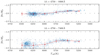 |
Fig. 7. [Fe/H]e vs. Teff relation obtained with GSL using different wavelength ranges of the observations. The top panel shows the relation for the full range, and the bottom panel shows the relation for the trimmed wavelength range (same as the MILES range in J20). The symbols and decorations are the same as in Fig 4. |
We have discussed the degeneracy between [Fe/H]e and [α/Fe] in the full wavelength range in Sect. 5.1. Comparing the solutions reported in Table 2 for the solar-scaled and enhanced models, we note that this degeneracy is a factor 2 smaller in the MILES range and 2.5 times smaller in the ELODIE range. This certainly reflects the dominance of the iron lines in the optical range.
6.2. Metallicity trend
A trend of the surface metallicity along the sequence of the cluster may be due to atomic diffusion. This is a balance between the gravitational settling and the radiative force that is counter-acted by the convective mixing. The resulting depletion of metals is larger at the TO, where the stars have thin convective layers. After the TO, these layers start to expand and to deepen, so that convection acts against atomic diffusion, re-homogenizing the matter (Salaris & Cassisi 2017). Consequently, the giant stars show the initial chemical composition at their surface. Theoretical models (e.g., Dotter et al. 2017) predict that the Fe abundance will be 0.1 − 0.2 dex lower at the TO. These models predict depletions that vary for the different atomic species.
In Korn et al. (2007) and Nordlander et al. (2012), a 0.1 dex depletion of Fe at the TO compared to the SGB of NGC 6397 was detected. They also measured similar trends for other elements (Mg, Ca, Ti, and Cr). The follow-up paper by Lind et al. (2008) confirmed the higher-resolution results. It should be noted that while the former results were derived from a non-LTE analysis, the latter are derived in LTE approximation: however, given the limited Teff range of the sample, the LTE correction is not expected to induce a metallicity trend. These trends, compared to models of atomic diffusion by Richard et al. (2005), allowed the authors to constrain the mixing parameters, which in turn could be used to derive the initial or primordial abundance of Li. Lovisi et al. (2012) independently re-analysed the latter dataset, and their results did not show the above [Fe/H] trend. Studies by other groups, albeit based on only a few stars, did show no or even opposite trends (Gratton et al. 2001; Koch & McWilliam 2011). Metallicity trends were subsequently detected in several other GCs by the same group. In NGC 6752, using similar data, Gruyters et al. (2013, 2014) found a Fe depletion of 0.08 ± 0.06 dex that is significant at the 1–2σ level. Finally, a similar depletion was found in M 30 (also known as NGC 7099; Gruyters et al. 2016; Gavel et al. 2021), a more distant cluster for which measuring abundances of TO stars is challenging.
In other clusters with similar spectroscopic measurements extending to the TO, no [Fe/H] trends were observed. This is the case in M 4 (also known as NGC 6121, with [Fe/H] = −1.1 dex) (Mucciarelli et al. 2011).
In our analysis, the trend (τ([Fe/H])) is reported in Table 2. With the two considered synthetic grids, [Fe/H]e increases from the TO along the SG. When the analysis is carried out over the full wavelength range and models are used that are enhanced in α-elements, we find τ([Fe/H])∼0.2 dex, which agrees with earlier results by H16. At first sight, it corroborates the earlier analyses of high-resolution spectra reported above. However, while we tend to have more confidence in the results based on the full spectral range because they have the best precision, we do not ignore the solutions obtained on the shortened optical range, which are notably different. They reach τ([Fe/H])∼0.3 − 0.4 dex (Figs. 7 and 8). As noted when we discussed the mean equivalent Fe abundance, there appears to exist a difference between the optical and NIR regions, and it is certainly due to imperfections in the synthetic spectra.
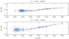 |
Fig. 8. [Fe/H]e vs. Teff relation obtained with AP18 grids ([α/Fe] = +0.5 dex) using different wavelength ranges of the observations: the full range (top panel), and the trimmed wavelength range (bottom panel). The symbols and decorations are the same as in Fig 4. |
The discrepancy pointed out in J20 between the nearly constant Fe abundance found with empirical libraries and the rising abundance obtained with synthetic libraries is even starker when the comparison is made over the same wavelength range. Our new analyses produced unrealistic values in some cases, in particular for the coolest stars analysed with AP18 ([Fe/H]e ∼ −1.6 dex).
The libraries used in J20 are sets of observations of real stars, and they provide a better spectral match with other observations than synthetic spectra do. However, these libraries had to be calibrated in Teff, log g, and [Fe/H] using classical methods based on high spectral resolution spectroscopy, and they therefore also rely on synthetic spectra. This means that the advantage of a better spectral match may to some extend be dampened by the uncertainties linked to this indirect calibration, and in particular its inhomogeneity resulting from the many sources of measurements used to build a library. A more arguable aspect of empirical libraries, however, is their limited coverage of the parameter space. J20 questioned the small number of low-metallicity stars in libraries as a possible source of the discrepancy.
On the other hand, synthetic libraries entail shortcomings in the lists of atomic or molecular lines or in the implementation of the physics in the models that are probably the origin of the poorer spectral match. They may also cause systematics on the derived parameters that might also explain the discrepancy.
The consistency between the solutions obtained with the two synthetic grids is an interesting point, but it does not disqualify the results of J20. The two types of reference libraries have their respective strengths and weaknesses, and at this point, we cannot conclude about the accuracy of the empirical or synthetic solutions. It would be premature to interpret our full-spectrum fitting analyses of low-resolution spectra in physical terms and claim the detection of signatures of atomic diffusion.
6.3. Cosmic metallicity spread
Some massive clusters, such as ω Cen, and Terzan 5, exhibit a large [Fe/H] spread (see e.g., Origlia et al. 2003; Ferraro et al. 2009) and are regarded as atypical. Most other clusters are homogeneous concerning iron: Carretta et al. (2009) assessed the [Fe/H] spread in GCs using medium-resolution (R = 20 000) spectra of 2000 stars in 19 clusters (about 100 stars in each cluster). They found a measured spread of 0.048 dex, dominated by the uncertainties on the measurements to a level at which it was impossible to measure reliable intrinsic values.
Mészáros et al. (2020) more recently reached the same conclusion from a homogeneous analysis of 30 clusters in the APOGEE survey. The compilation by Bailin (2019) reported 55 clusters with a possibly detected [Fe/H] spread with a median value of 0.045 dex. However, this is comparable to the errors on individual measurements and therefore critically depends on a precise knowledge of them (in this case, the errors are essentially derived from the dispersion of the measurements obtained on individual spectral lines; by ignoring the propagation of the random errors on the atmospheric parameters, the errors may have been under-estimated and the spread over-estimated). In some clusters, spreads of ∼0.05 dex were claimed, but later disputed (see e.g., Mucciarelli et al. 2015, in NGC 6656), reflecting the caveat of precision abundances measurements. For about 40 giants in NGC 6752, Yong et al. (2013) carried out a relatively detailed abundances analysis using high-resolution spectra. They achieved an internal precision of about 0.01 dex and measured a 0.02 dex spread for [Fe/H]. These small spreads may be more representative of the general population of Galactic cluster, but He variation could also contribute to this apparent spread. In contrast, spreads in lighter elements with amplitudes reaching 0.1 dex are widely observed (e.g., Carretta et al. 2009), and are certainly associated with the presence of multiple stellar populations.
In our analysis, the squared difference between the measured spread and the dispersion due to the noise and data reduction, ![Mathematical equation: $ \Delta(\mathrm{[Fe/H]}) = \sqrt{ \sigma(\mathrm{[Fe/H]})^2 - \epsilon(\mathrm{[Fe/H]})^2} $](/articles/aa/full_html/2022/05/aa42667-21/aa42667-21-eq2.gif) , reflects the other causes of uncertainty and the intrinsic equivalent [Fe/H]e spread. Considering the fits giving the smallest ϵ([Fe/H]) in Table 2, those over the full wavelength range with either GSL or AP18, the residual spread is Δ([Fe/H]) = 0.057 dex. If we consider the J20 solution, we obtain a similar estimate: Δ([Fe/H]) = 0.054 dex (although it is based on a shorter wavelength range, this solution has a precision comparable to that of the synthetic libraries on the full wavelength range). This is an upper limit to the intrinsic spread in equivalent [Fe/H]e, but the consistency between the two estimates suggests that it is close to the real value.
, reflects the other causes of uncertainty and the intrinsic equivalent [Fe/H]e spread. Considering the fits giving the smallest ϵ([Fe/H]) in Table 2, those over the full wavelength range with either GSL or AP18, the residual spread is Δ([Fe/H]) = 0.057 dex. If we consider the J20 solution, we obtain a similar estimate: Δ([Fe/H]) = 0.054 dex (although it is based on a shorter wavelength range, this solution has a precision comparable to that of the synthetic libraries on the full wavelength range). This is an upper limit to the intrinsic spread in equivalent [Fe/H]e, but the consistency between the two estimates suggests that it is close to the real value.
Δ([Fe/H]) combines the spread on the iron abundance and the effect of the spread on other elements. We discussed the degeneracy between [Fe/H]e and [α/Fe] above. A change in δ[α/Fe] results in a δ[Fe/H] change in δ[Fe/H] = a × δ[α/Fe], where according to the values in Table 2, a = 0.58 for GSL and a = 0.75 for AP18. An intrinsic [α/Fe] spread of ∼0.08 − 0.1 dex would therefore be sufficient to explain Δ([Fe/H]). This value is possible, and the observed residual spread does not require a spread of iron abundance.
7. Conclusion
We re-analysed the MUSE commissioning observations of 1061 stars in NGC 6397 previously studied by H16 and J20 in order to evaluate whether such a large set of low-resolution (R ∼ 2000) spectra may allow us to probe subtle effects in the stellar atmospheres. In particular, our aim was to determine whether variations in the surface chemical composition along the sequence of the cluster may be reliably studied or if they remain masked by effects due to the analysis procedures or to the modelling of the spectra.
Specifically, we focused on the disagreement between H16 and J20 on the [Fe/H]e trend: H16 found that the equivalent iron abundance rises by about 0.15 dex along the SG branch, while J20 did not find any trend. The two studies used the same data and similar analysis methods, but the first used as reference the GSL grid of synthetic spectra and the second used empirical libraries (ELODIE and MILES). The open questions were (i) whether the details of the analysis procedure, for instance the interpolation between spectra within the grid, affect the measured metallicty trend and (ii) whether the spectral models of stellar atmospheres have the required reliability to reveal the fine physical details.
Our analysis was made with a different code, FERRE. This code allowed us to explore the importance of the interpolation schema and different grids of models, GSL and AP18, which enabled us to explore the effect of the mesh size.
We found that (i) the interpolation schema and grid sampling are not critical with the considered grids, and (ii) GSL and AP18 are essentially consistent for the measured iron abundance trend: In both cases, we find an abundance increase along the SG branch, which also agrees with the results of H16; and (iii) the precision of the measurements is mostly similar with both grids, although it is marginally better with AP18. When it is restricted to the optical wavelength range, the precision is strongly degraded and does not rival the precision reached by J20 using empirical libraries.
Therefore, we give a robust and unambiguous answer to the first question: The interpolation is not an issue, even for interpreting abundance trends that are one-fivth or one-tenth of the mesh size. A linear approximation of the variations in the grid is still satisfactory, although cubic interpolations are better.
The second question is more difficult. The consistency between the results obtained with the two grids of models is encouraging, but does not formally imply that the results are reliable. It remains risky to simply reject the results obtained by J20 with empirical libraries. Although these latter libraries are used at the edge of their validity space and the results stand on a limited number of reference stars with well-documented parameters, the nearly constant iron abundance found with both MILES and ELODIE is striking. Nothing in the process biases the result towards a constant abundance, and the probability of obtaining this result by chance is certainly low. In addition, the quality of the spectral fits is considerably better with the empirical libraries, and the abundance uncertainties and spread are smaller.
We recall that the GSL and AP18 models share some physical assumptions and ingredients. In particular, the atomic and molecular line lists have similar limitations that may explain a large part of the observed spectral residuals. The difference observed between the solutions obtained in the optical and in the optical plus NIR (see Sect. 6.1) indicates that the models are not yet accurate enough. Metallicity biases of 0.1 or 0.2 dex are possible, and the divergence of the iron abundance trend when the wavelength range is shortened (in particular with AP18) casts some doubts on the reality of this trend.
In contrast, we found the trend to be relatively robust toward the choice of the micro-turbulence velocity parameter and of its variation along the cluster sequence. The possible effect is only ∼0.03 dex on τ([Fe/H]).
The difference between synthetic and empirical libraries is not explained, and there are still some open questions that need to be further investigated in the future. The use of the X-Shooter Spectral Library (Gonneau et al. 2020; Verro et al. 2022) to fit the whole wavelength range may help to shed light on the current difference observed between optical and NIR. Our dataset comes from short exposures, and therefore the achieved S/N is not the best that could be obtained with the instrument. The observed spread is definitely dominated by the effect of the noise. With better observations, the main source of error may be lowered, which would improve the determination of the intrinsic equivalent iron abundance spread. It may also allow us to separate the [α/Fe] and [Fe/H] spreads. Improving the synthetic models is a more difficult and critical issue. One route could be the empirical calibration of the atomic and molecular line lists (Martins et al. 2014; Shetrone et al. 2015; Franchini et al. 2018), but this may mask some more fundamental questions in the stellar models, such as the effects of non-LTE or 3D treatment.
We checked that the other minimisation algorithms accurately produce the same results for any interpolation scheme. Therefore, we adopt this default algorithm, and will not discuss the other algorithms.
FERRE also proposes a method called “cubic spline”, based on Press et al. (1992), but while the scope of the cubic spline is to provide an interpolating function with continuous first and second derivatives over the whole range of the parameters, the implementation is “local” (solved in each dimension in a four-point neighbourhood).
The original grid was limited to Teff ≤ 8000 K. The version available on the website extends the grid to hotter models.
This aspect, not fundamental to the FERRE principle, is due to the choice of describing the grid with a simple coordinate system.
Acknowledgments
We thank the anonymous referee for very helpful comments and suggestions. We thank Tim-Oliver Husser who shared with us the tables with the results of the H16 analysis, and the MUSE team for making public the extracted spectra on their website. We are grateful to Lucimara Martins, Ariane Lançon, Anke Arentsen, Paula Coelho, and Rashi Jain for fruitful discussions. We acknowledge the LABEX Lyon Institute of Origins (ANR-10-LABX-0066) of the Université de Lyon for its support within the program “Investissements d’Avenir” (ANR-11-IDEX-0007) of the French government operated by the National Research Agency (ANR), IUCAA and CRAL for their support for the IFAS summer school where this work was started. This work was supported in part by grant ANR-19-CE31-0022 (POPSYCLE) of the French ANR.
References
- Allende-Prieto, C., & Apogee Team 2015, in Am. Astron. Soc. Meeting Abstr., 225, 422.07 [NASA ADS] [Google Scholar]
- Allende Prieto, C., Koesterke, L., Hubeny, I., et al. 2018, A&A, 618, A25 [NASA ADS] [CrossRef] [EDP Sciences] [Google Scholar]
- Anderson, J., Sarajedini, A., Bedin, L. R., et al. 2008, AJ, 135, 2055 [Google Scholar]
- Asplund, M., Grevesse, N., Sauval, A. J., & Scott, P. 2009, ARA&A, 47, 481 [NASA ADS] [CrossRef] [Google Scholar]
- Auer, L. 2003, in Stellar Atmosphere Modeling, eds. I. Hubeny, D. Mihalas, & K. Werner, 288, 3 [NASA ADS] [Google Scholar]
- Bacon, R., Accardo, M., Adjali, L., et al. 2010, in Ground-based and Airborne Instrumentation for Astronomy III, eds. I. S. McLean, S. K. Ramsay, & H. Takami, SPIE Conf. Ser., 7735, 773508 [Google Scholar]
- Bailin, J. 2019, ApJS, 245, 5 [NASA ADS] [CrossRef] [Google Scholar]
- Bressan, A., Marigo, P., Girardi, L., et al. 2012, MNRAS, 427, 127 [NASA ADS] [CrossRef] [Google Scholar]
- Carretta, E., Bragaglia, A., Gratton, R., D’Orazi, V., & Lucatello, S. 2009, A&A, 508, 695 [NASA ADS] [CrossRef] [EDP Sciences] [Google Scholar]
- Chapman, S. 1917, MNRAS, 77, 540 [NASA ADS] [CrossRef] [Google Scholar]
- Dotter, A., Conroy, C., Cargile, P., & Asplund, M. 2017, ApJ, 840, 99 [Google Scholar]
- Ferraro, F. R., Dalessandro, E., Mucciarelli, A., et al. 2009, Nature, 462, 483 [Google Scholar]
- Franchini, M., Morossi, C., Di Marcantonio, P., et al. 2018, ApJ, 862, 146 [Google Scholar]
- García Pérez, A. E., Allende Prieto, C., Holtzman, J. A., et al. 2016, AJ, 151, 144 [Google Scholar]
- Gavel, A., Gruyters, P., Heiter, U., et al. 2021, A&A, 652, A75 [NASA ADS] [CrossRef] [EDP Sciences] [Google Scholar]
- Gilmore, G., Randich, S., Asplund, M., et al. 2012, Messenger, 147, 25 [Google Scholar]
- Gonneau, A., Lyubenova, M., Lançon, A., et al. 2020, A&A, 634, A133 [NASA ADS] [CrossRef] [EDP Sciences] [Google Scholar]
- Gratton, R. G., Bonifacio, P., Bragaglia, A., et al. 2001, A&A, 369, 87 [NASA ADS] [CrossRef] [EDP Sciences] [Google Scholar]
- Gratton, R. G., Carretta, E., & Bragaglia, A. 2012, A&ARv, 20, 50 [CrossRef] [Google Scholar]
- Gray, R. O., Graham, P. W., & Hoyt, S. R. 2001, AJ, 121, 2159 [NASA ADS] [CrossRef] [Google Scholar]
- Gruyters, P., Korn, A. J., Richard, O., et al. 2013, A&A, 555, A31 [NASA ADS] [CrossRef] [EDP Sciences] [Google Scholar]
- Gruyters, P., Nordlander, T., & Korn, A. J. 2014, A&A, 567, A72 [NASA ADS] [CrossRef] [EDP Sciences] [Google Scholar]
- Gruyters, P., Lind, K., Richard, O., et al. 2016, A&A, 589, A61 [NASA ADS] [CrossRef] [EDP Sciences] [Google Scholar]
- Gustafsson, B., Edvardsson, B., Eriksson, K., et al. 2008, A&A, 486, 951 [NASA ADS] [CrossRef] [EDP Sciences] [Google Scholar]
- Harris, W. E. 2010, ArXiv e-prints [arXiv:1012.3224] [Google Scholar]
- Hauschildt, P. H., & Baron, E. 1999, J. Comput. Appl. Math., 109, 41 [NASA ADS] [CrossRef] [Google Scholar]
- Husser, T. O., Wende-von Berg, S., Dreizler, S., et al. 2013, A&A, 553, A6 [NASA ADS] [CrossRef] [EDP Sciences] [Google Scholar]
- Husser, T.-O., Kamann, S., Dreizler, S., et al. 2016, A&A, 588, A148 [NASA ADS] [CrossRef] [EDP Sciences] [Google Scholar]
- Jain, R., Prugniel, P., Martins, L., & Lançon, A. 2020, A&A, 635, A161 [EDP Sciences] [Google Scholar]
- Kamann, S., Wisotzki, L., & Roth, M. M. 2013, A&A, 549, A71 [NASA ADS] [CrossRef] [EDP Sciences] [Google Scholar]
- Koch, A., & McWilliam, A. 2011, AJ, 142, 63 [NASA ADS] [CrossRef] [Google Scholar]
- Koesterke, L. 2009, in Recent Directions in Astrophysical Quantitative Spectroscopy and Radiation Hydrodynamics, eds. I. Hubeny, J. M. Stone, K. MacGregor, & K. Werner, Am. Inst. Phys. Conf. Ser., 1171, 73 [NASA ADS] [Google Scholar]
- Koleva, M., Prugniel, P., Bouchard, A., & Wu, Y. 2009, A&A, 501, 1269 [CrossRef] [EDP Sciences] [Google Scholar]
- Korn, A. J., Grundahl, F., Richard, O., et al. 2007, ApJ, 671, 402 [NASA ADS] [CrossRef] [Google Scholar]
- Kurucz, R. L. 2009, in Recent Directions in Astrophysical Quantitative Spectroscopy and Radiation Hydrodynamics, eds. I. Hubeny, J. M. Stone, K. MacGregor, & K. Werner, Am. Inst. Phys. Conf. Ser., 1171, 43 [NASA ADS] [Google Scholar]
- Lançon, A., Gonneau, A., Verro, K., et al. 2021, A&A, 649, A97 [NASA ADS] [CrossRef] [EDP Sciences] [Google Scholar]
- Lee, Y. S., Beers, T. C., Sivarani, T., et al. 2008, AJ, 136, 2022 [Google Scholar]
- Leibniz, G. W. 1765, New Essay on Human Understanding (Book IV, Chapter 16) [Google Scholar]
- Lind, K., Korn, A. J., Barklem, P. S., & Grundahl, F. 2008, A&A, 490, 777 [NASA ADS] [CrossRef] [EDP Sciences] [Google Scholar]
- Lovisi, L., Mucciarelli, A., Lanzoni, B., et al. 2012, ApJ, 754, 91 [Google Scholar]
- Martins, L. P., & Coelho, P. 2007, MNRAS, 381, 1329 [Google Scholar]
- Martins, L. P., Coelho, P., Caproni, A., & Vitoriano, R. 2014, MNRAS, 442, 1294 [NASA ADS] [CrossRef] [Google Scholar]
- Martins, L. P., Lima-Dias, C., Coelho, P. R. T., & Laganá, T. F. 2019, MNRAS, 484, 2388 [NASA ADS] [CrossRef] [Google Scholar]
- Mészáros, S., & Allende Prieto, C. 2013, MNRAS, 430, 3285 [CrossRef] [Google Scholar]
- Mészáros, S., Allende Prieto, C., Edvardsson, B., et al. 2012, AJ, 144, 120 [Google Scholar]
- Mészáros, S., Martell, S. L., Shetrone, M., et al. 2015, AJ, 149, 153 [Google Scholar]
- Mészáros, S., Masseron, T., García-Hernández, D. A., et al. 2020, MNRAS, 492, 1641 [Google Scholar]
- Mucciarelli, A. 2011, A&A, 528, A44 [NASA ADS] [CrossRef] [EDP Sciences] [Google Scholar]
- Mucciarelli, A., Salaris, M., Lovisi, L., et al. 2011, MNRAS, 412, 81 [NASA ADS] [CrossRef] [Google Scholar]
- Mucciarelli, A., Lapenna, E., Massari, D., et al. 2015, ApJ, 809, 128 [NASA ADS] [CrossRef] [Google Scholar]
- Nordlander, T., Korn, A. J., Richard, O., & Lind, K. 2012, ApJ, 753, 48 [NASA ADS] [CrossRef] [Google Scholar]
- Origlia, L., Ferraro, F. R., Bellazzini, M., & Pancino, E. 2003, ApJ, 591, 916 [Google Scholar]
- Press, W. H., Teukolsky, S. A., Vetterling, W. T., & Flannery, B. P. 1992, Numerical Recipes in Fortran 77, 2nd edn. (Cambridge, USA: Cambridge University Press) [Google Scholar]
- Prugniel, P., & Soubiran, C. 2001, A&A, 369, 1048 [CrossRef] [EDP Sciences] [Google Scholar]
- Richard, O., Michaud, G., & Richer, J. 2005, ApJ, 619, 538 [Google Scholar]
- Salaris, M., & Cassisi, S. 2017, R. Soc. Open Sci., 4, 170192 [Google Scholar]
- Sánchez-Blázquez, P., Peletier, R. F., Jiménez-Vicente, J., et al. 2006, MNRAS, 371, 703 [Google Scholar]
- Shetrone, M., Bizyaev, D., Lawler, J. E., et al. 2015, ApJS, 221, 24 [Google Scholar]
- Takeda, Y., Sato, B., & Murata, D. 2008, PASJ, 60, 781 [NASA ADS] [CrossRef] [Google Scholar]
- Verro, K., Trager, S. C., Peletier, R. F., et al. 2022, A&A, 660, A34 [NASA ADS] [CrossRef] [EDP Sciences] [Google Scholar]
- Wu, Y., Singh, H. P., Prugniel, P., Gupta, R., & Koleva, M. 2011, A&A, 525, A71 [NASA ADS] [CrossRef] [EDP Sciences] [Google Scholar]
- Yong, D., Meléndez, J., Grundahl, F., et al. 2013, MNRAS, 434, 3542 [NASA ADS] [CrossRef] [Google Scholar]
Appendix A: Discontinuity and outliers in GSL
Natura non facit saltum (nature does not make jumps, Leibniz 1765) expresses a “continuity principle” that has been called along the centuries to justify or describe important theories in various fields of sciences, from the infinitesimal calculus to the evolution of biological organisms. If not a strong physical law, this is definitely an assumption behind interpolating in a grid of models to determine physical parameters. In the considered region of parameters, the stellar spectra are continuous with respect to Teff, log g, and chemical composition, but artificial discontinuities, irregularities, or outlier spectra may arise from the modelling. The irregular distribution of the measurements along the cluster sequence (see H16 their figure 8 and J20 their figure 1) suggests such discontinuities: there are gaps and concentrations in the Teff coverage, in particular, near Teff = 5000 K. Tim-Oliver Husser reported suspicions of problems in GSL in this region for giant stars (private communication).
Therefore, we explored the grid in search for outliers or discontinuities. For each log g, [Fe/H], and [α/Fe], we computed the difference between a spectrum on the grid and a spectrum that was linearly interpolated using the preceding and following spectra along the temperature sequence. This allowed us to clearly detect a sharp discontinuity separating the region with Teff ≤ 5000 K from the rest (this affects the entire range of gravities, not only the giants). We also found isolated outliers at [Teff, log g, [Fe/H]]=[5400, 2.0, −1.5],[6900, 2.0, −1.5], and [5600, 2.0, −3.0], which are too far from the cluster sequence to affect our analysis, and also at [6400, 4., − 2], [6300, 4., − 1.5], [6400, 4., − 3]. These latter outliers, and in particular the first, may affect the measurements near the TO and may be due to undiagnosed failure in the convergence of the models. Some convergence issues due to numerical instabilities where the convection layer is thin are identified in the header of the GSL files, and in some cases, the convection has been disabled and/or the ξ parameter set to zero, but this affects warm giants, not the outliers detected here. ======= In the considered region of parameters, the stellar spectra are continuous with respect to Teff, log g, and chemical composition, but artificial discontinuities, irregularities, or outliers in spectra may arise from the modelling. The irregular distribution of the measurements along the cluster’s sequence (see H16 their figure 8 and J20 their figure 1) suggests such discontinuities: there are gaps and concentrations in the Teff coverage, in particular, near Teff = 5000 K. Tim-Oliver Husser reported to us suspicions of problems in GSL in this region for giant stars (private communication).
Therefore, we explored the grid in search for outliers or discontinuities. For each log g, [Fe/H], and [α/Fe], we computed the difference between a spectrum on the grid, and the one linearly interpolated using the preceding and following spectra along the temperature sequence. This allowed us to clearly detect a sharp discontinuity separating the region with Teff ≤ 5000 K from the rest (this affects all the range of gravities, not only the giants). We also found isolated outliers at [Teff, log g, [Fe/H]]=[5400, 2.0, −1.5],[6900, 2.0, −1.5], and [5600, 2.0, −3.0], which are too far from the cluster’s sequence to affect our analysis, and also at [6400, 4., − 2], [6300, 4., − 1.5], [6400, 4., − 3]. These latter outliers, and in particular the first one, may affect the measurements near the TO, and may be due to undiagnosed failure in the convergence of the models. Some convergence issues, due to numerical instabilities where the convection layer is thin are identified in the header of the GSL files, and in some cases the convection has been disabled and/or the ξ parameter set to zero; but this affects warm giants, and not the outliers detected here.
To study the discontinuity at Teff = 5000 K further, we selected spectra from J20 with 4300 < Teff < 5300 K and used FERRE to build χ2 maps. For each point of a Teff versus log g grid, we linearly interpolated a spectrum in GSL at the log g obtained in J20, and we computed the corresponding χ2 value. An example of the resulting χ2 map is presented in the right panel of Fig. A.1 for the spectrum ID = id000009229jd2456865p5898f000. The map shows a step where the region with Teff ≤ 5000 K has a higher χ2, that is, the quality of the grid is lower in the low-temperature regime, and the temperature of the minimum χ2, Teff = 5035 K has been biased toward a higher value. The left panel presents the stacked χ2 map for the 214 spectra with 4300 < Teff < 5300 K. The stacking shows that the problem is not due to an individual spectrum, and is definitely a sharp step in the χ2 space. The transition in the range 5000 < Teff < 5100 K is due to the linear interpolation used in the visualisation process.
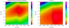 |
Fig. A.1. χ2 map with GSL in the region of the Teff = 5000 K discontinuity. On the right, we show the spectrum ID = id000009229jd2456865p5898f000 in the full wavelength range. On the left, we show a stacked map for the 214 spectra with 4300 < Teff < 5300 K, selected from J20. |
We are not certain about the origin of this discontinuity, but the GSL paper (Husser et al. 2013) mentions that above 5000 K the reference wavelength used to determine the mean optical depth changes from 12 000 Å to 5 000 Å. Other discontinuities of the parameters are also mentioned at 4000 K and 8000 K, but because they are not in the region of interest for the present work, we did not explore them and we cannot report whether they are associated with discontinuities in the spectra. The first is a threshold above which NLTE corrections are used in the computations of some line profiles, and the second marks the temperature over which the molecular line list is limited to a few important species.
Lançon et al. (2021) carried out an extensive comparison between the empirical X-Shooter Spectral Library (Gonneau et al. 2020, XSL) and GSL, and found discrepancies arising below Teff = 5000 K, particularly in the blue region of the spectra. It is difficult to precisely relate this degradation to the discontinuity we observe, however. There are indeed a number of reasons why the model matches become more problematic at low temperature. We limited the range of our grids to Teff ≥ 5100 K in order to avoid problems with the interpolation at cooler temperatures.
Appendix B: Interpolation artefacts
As mentioned in Sect. 4.4, there are obvious concentrations of points at [Fe/H] = −2.0 dex (a slice of the grid) in Fig. 4 where the analysis was made with GSL. The same pattern is seen in Fig. 6, with a second concentration at [Fe/H] = −2.25 dex, also a slice for the AP18 grid. These patterns are particularly visible with the linear interpolation, but they also present with the quadratic interpolation (as already noticed by García Pérez et al. 2016, who analysed the APOGEE data with FERRE). These are artefacts of the interpolation methods.
Whether it explicitly computes the derivatives or not, the minimisation algorithm descends the slope, and may get contradictory indications on the two sides of a slice where the derivatives are discontinuous. This may cause the solution to diverge from the slice (which is not seen in the distribution of the solutions), or to converge to the slice and produce concentration of points aligned on slices. This difficulty is inherent to any local interpolation, regardless of its order, as they are by nature non-derivable at the nodes. However, with higher-order interpolation, the problem becomes smaller, certainly because the discontinuities are reduced. It is barely apparent with the quadratic interpolation and is invisible with the cubic one. A global spline interpolation would avoid this artefact. These concentrations will often not bias the solutions statistically: although they are easily detected on graphs, they may concern only a small fraction of the solutions and affect a very limited region of the parameter space in the close vicinity of a slice of the grid.
All Tables
Mean iron abundance, errors, dispersion, and trend obtained from different setups, compared with H16 and J20.
All Figures
|
Fig. 1. Parameter space coverage of the grids. The grey dots represent the analysed sample, and the black dots mark the nodes of the grids of synthetic spectra. The top panels are the projections on the log g vs. Teff plane, and the bottom panels show the projections in [Fe/H] vs. Teff. The left column is for the GSL (the [Fe/H] = −2.5 dex slice, which is not originally a part of GSL, and is produced by averaging the [Fe/H] = −3 dex and [Fe/H] = −2 dex slices, see Sect. 4). The central column is the AP18 grid (see Sect. 5). The right column is also from the AP18 grid, but with twice larger steps on each axis to evaluate the effect of a coarser grid (see Sect. 5.2). |
| In the text | |
|
Fig. 2. Typical fits of a spectrum (ID = id000010747jd2456866p4985f000). The fit, performed over the complete wavelength range, 4750–9300 Å, returned Teff = 5471 K and [Fe/H]e = −1.84 dex for global rms residuals of 0.01 for both GSL and AP18. The left column shows the [α/Fe] = 0.4 dex GSL grid, and the right column presents the [α/Fe] = 0.5 dex fine AP18 grid. The top row shows a small wavelength region around the Hβ line, the middle row shows a region around the Mgb triplet, and the bottom one shows a region around the Ca II triplet. For each plot, the top panel presents the observation (black line) with the best-fit model over-plotted in red. The bottom panel presents the residuals, observation minus model. |
| In the text | |
|
Fig. 3. Comparison between our measurements (y-axis) and H16 results (x-axis) obtained with solar [α/Fe]. Bottom panels: differences Δ (our − H16). We report the comparison between the Teff on the left and the comparison between our [Fe/H]e and [Fe/H] of H16 on the right. The mean and rms differences are indicated. |
| In the text | |
|
Fig. 4. [Fe/H]e vs. Teff diagrams published in H16 (top panel, with [α/Fe] = 0) and those obtained with FERRE using GSL and the three different interpolation schemes (other panels, with [α/Fe] = +0.4). The measurements of individual spectra are shown as blue dots, and the nodes of the grids are overlaid as thin crosses. The red dots and line are the mean [Fe/H]e in bins of 250 K, and the error bars are the dispersion in these bins. |
| In the text | |
|
Fig. 5. Comparison between Teff and [Fe/H]e obtained with GSL and AP18 grids. Top panel: difference between Teff (ΔTeff(AP18-GSL), computed by subtracting the GSL results from the AP18 results) as a function of Teff values with GSL. Bottom panel: difference of equivalent iron abundance (Δ[Fe/H]e) as a function of the iron abundance with GSL. The dashed blue line shows the expected bias due to the different level of α-element enhancement in the two grids (0.4 vs. 0.5 dex, see the text for details). In both panels we report the mean and rms of the differences. |
| In the text | |
|
Fig. 6. [Fe/H]e vs. Teff relation using the AP18 fine (top and second panels) and coarse (third panel) grids. The top panel shows the linear interpolation, and the two other panels show the cubic interpolation. The grey lines and symbols represent the solution (with an offset of −0.076) obtained with the GSL grid (cubic interpolation) and reported on Fig. 4. The other symbols and line styles are as in Fig. 4. |
| In the text | |
|
Fig. 7. [Fe/H]e vs. Teff relation obtained with GSL using different wavelength ranges of the observations. The top panel shows the relation for the full range, and the bottom panel shows the relation for the trimmed wavelength range (same as the MILES range in J20). The symbols and decorations are the same as in Fig 4. |
| In the text | |
|
Fig. 8. [Fe/H]e vs. Teff relation obtained with AP18 grids ([α/Fe] = +0.5 dex) using different wavelength ranges of the observations: the full range (top panel), and the trimmed wavelength range (bottom panel). The symbols and decorations are the same as in Fig 4. |
| In the text | |
|
Fig. A.1. χ2 map with GSL in the region of the Teff = 5000 K discontinuity. On the right, we show the spectrum ID = id000009229jd2456865p5898f000 in the full wavelength range. On the left, we show a stacked map for the 214 spectra with 4300 < Teff < 5300 K, selected from J20. |
| In the text | |
Current usage metrics show cumulative count of Article Views (full-text article views including HTML views, PDF and ePub downloads, according to the available data) and Abstracts Views on Vision4Press platform.
Data correspond to usage on the plateform after 2015. The current usage metrics is available 48-96 hours after online publication and is updated daily on week days.
Initial download of the metrics may take a while.