| Issue |
A&A
Volume 661, May 2022
|
|
|---|---|---|
| Article Number | A79 | |
| Number of page(s) | 15 | |
| Section | Stellar atmospheres | |
| DOI | https://doi.org/10.1051/0004-6361/202142298 | |
| Published online | 17 May 2022 | |
X-ray activity of the young solar-like star Kepler-63 and the structure of its corona
1
Institut für Astronomie und Astrophysik Tübingen, Kepler Center for Astro and Particle Physics, Eberhard Karls Universität,
Sand 1,
72076
Tübingen,
Germany
e-mail: This email address is being protected from spambots. You need JavaScript enabled to view it.
2
INAF – Osservatorio Astronomico di Palermo,
Piazza del Parlamento 1,
90134
Palermo,
Italy
Received:
24
September
2021
Accepted:
10
February
2022
Abstract
The X-ray satellite XMM-Newton has so far revealed coronal cycles in seven solar-like stars. Of these, the youngest stars ϵ Eridani (~400 Myr) and ι Horologii (~600 Myr) display the shortest X-ray cycles and the smallest amplitudes, defined as the variation of the X-ray luminosity between the maximum and minimum of the cycle. The X-ray cycle of ϵ Eridani was characterised by applying a novel technique that allowed us to model the corona of a solar-like star in terms of magnetic structures, such as those observed on the Sun (active regions, cores of active regions, and flares), at various filling factors. The high surface coverage of the magnetic structures on ϵ Eridani (65%–95%) that emerged from that study was suggested to be responsible for the low cycle amplitude in the X-ray band. It was also hypothesised that the basal surface coverage with magnetic structures may be higher on the corona of solar-like stars while they are young. To investigate this hypothesis, we started the X-ray monitoring campaign of Kepler-63 in 2019. The star had been observed once before, in 2014, with XMM-Newton. With an age of 210 ± 45 Myr and a photospheric cycle of 1.27 yr, Kepler-63 is the youngest star so far to be observed in X-rays in order to reveal its coronal cycle. Our campaign comprised four X-ray observations of Kepler-63 spanning 10 months (i.e. three-fifths of its photospheric cycle). The long-term X-ray light curve did not reveal a periodic variation of the X-ray luminosity, but a factor two change would be compatible with the considerable uncertainties in the low signal-to-noise data for this relatively distant star. In the case of ϵ Eridani, we describe the coronal emission measure distribution (EMD) of Kepler-63 with magnetic structures such as those observed on the Sun. The best match with the observations is found for an EMD composed of cores and flares of GOES Class C and M following the canonical flare frequency distribution. More energetic flares are occasionally present but they do not contribute significantly to the quasi-stationary high-energy component of the emission measure probed with our modelling. This model yields a coronal filling factor of 100%. This complete coverage of the corona with X-ray-emitting magnetic structures is consistent with the absence of an X-ray cycle, confirming the analogous results derived earlier for ϵ Eridani. Finally, combining our results with the literature on stellar X-ray cycles, we establish an empirical relation between the cycle amplitude LX,max/LX,min and the X-ray surface flux, FX,surf. From the absence of a coronal cycle in Kepler-63, we infer that stars with higher X-ray flux than Kepler-63 must host an EMD that comprises a significant fraction of higher energy flares than those necessary to model the corona of Kepler-63, that is, flares of Class X or higher. Our study opens a new path for studies of the solar-stellar analogy and the joint exploration of resolved and unresolved variability in stellar X-ray light curves.
Key words: X-rays: stars / stars: activity / stars: coronae / stars: solar-type / stars: individual: Kepler 63
© ESO 2022
1 Introduction
The magnetic field in solar-like stars is maintained by the so-called α – Ω dynamo, which is responsible for periodically changing the configuration of the magnetic field lines. The timescale on which these changes take place defines the length of the activity cycle (Böhm-Vitense 2007). A consequence of the magnetic field re-configuration is the formation of magnetic structures that rise on the stellar surface, and evolve and decay periodically in the course of the magnetic cycle. The surface coverage with these structures therefore varies continuously between a minimum and a maximum. Therefore, by tracing the evolution of the magnetic structures we can characterise the activity cycles of solar-like stars. These structures are manifest in all layers of the stellar atmosphere, from the photosphere to the corona. Because of the temperature gradient that characterises the solar and stellar atmospheres, triggering different emission mechanisms for each layer of the atmosphere, activity cycles are expected to be found at different wavelengths, from the optical to the X-rays.
Photospheric and chromospheric cycles are well studied. In particular, ~60% of the main sequence stars show chromospheric cycles with periods lasting up to 20 yr (Wilson 1978). These cycles are characterised with Ca II H and K emission lines emitted by plages in the chromosphere. The photospheric cycles can instead be characterised by tracing the evolution of the starspots. One way of gathering information on the starspot evolution is the so-called spot transit method (Silva 2003), which infers the presence of starspots through the brightness changes during a planet transit.
Our knowledge about cycles in the outermost atmospheric layer, the corona, is still scarce. As the same dynamo process is responsible for the magnetic cycle in all parts of the stellar atmosphere, the length of X-ray cycles is expected to coincide with that of the chromospheric cycles. The latter have been seen to last up to 20 yr, and so long X-ray monitoring campaigns would be required to detect their coronal counterparts. Moreover, the search for X-ray cycles relies on sparsely sampled light curves. This is clearly a disadvantage for reliable coronal cycle detections. Therefore, studies of long-term X-ray variability have focused on stars with a known chromospheric cycle.
To date we are aware of the existence of only seven stars that show an X-ray activity cycle, all detected by the X-ray satellite XMM-Newton. For most of them, the common denominator is their age and the period of their coronal cycles. These stars are α Centauri A and B (Robrade et al. 2012), 61 Cygnus A and B (Hempelmann et al. 2006; Robrade et al. 2012), HD 81809 (Favata et al. 2008; Orlando et al. 2017), with ages between 3 and 6 Gyr and with X-ray activity cycles that last from 7 up to 20 yr. The remaining two stars with observed X-ray cycle, ι Horologii (Sanz-Forcada et al. 2013, 2019) and ϵ Eridani (Coffaro et al. 2020), are young stars, with ages of 600 and 400 Myr and with short coronal cycles that have periods of 1.6 and 2.9 yr, respectively. Moreover, these two young stars show another intriguing characteristic: the amplitude of their X-ray cycles, i.e. the variation of the X-ray luminosity between the minimum and maximum of their coronal emission, is remarkably small.
The X-ray emission of the Sun throughout its cycle is related to magnetic structures whose coronal coverage fraction changes along with the solar cycle. Exploiting the solar-stellar analogy, the hypothesis is that, for solar-like stars, we can link their X-ray variability to the same phenomenon. In this context, Coffaro et al. (2020) applied a novel technique which enables the X-ray emission of a star to be reproduced from time-variations in the coverage of its corona by the same kinds of magnetic structures that are observed on the Sun. This technique was developed in the framework of the study “The Sun as an X-ray star” (Orlando et al. 2000, 2001; Peres et al. 2000; Reale et al. 2001; see Sect. 3.1) in which observations of the solar corona by the X-ray satellite Yohkoh were converted into an almost identical format to that of the observations obtained with non-solar X-ray satellites, such as XXMM-Newton. The final data products of this method are synthetic X-ray spectra that are distinguished by a particular fractional coverage of magnetic structures on the corona, and can be directly compared to the observed spectra of a star with an active corona: from such a comparison, a percentage surface coverage with solar magnetic structures can be inferred for each stellar X-ray observation.
This method was first applied to HD81809 (Orlando et al. 2017). A more detailed study was carried out by Coffaro et al. (2020) for ϵ Eridani. In that work we revealed the significant presence of magnetic structures on the corona throughout the X-ray activity cycle of ϵ Eridani. We argued that the high level of coverage of the corona by these magnetic structures (from ~70 to ~90%) does not allow the X-ray luminosity to significantly vary during the coronal cycle, explaining the small amplitude of the X-ray luminosity from ϵ Eridani.
To better understand the origin of small cycle amplitudes and to investigate whether or not solar-like stars younger than ϵ Eridani show X-ray activity cycles, we began the study of Kepler-63, a young G2V star at a distance of 200 pc. With its age of 210 ± 45 Myr (Sanchis-Ojeda et al. 2013), it is younger than the other stars that show short coronal activity cycles. It is also a fast rotator, with a rotational period of ~5.4 days and hosts a Jupiter-like planet with a polar orbit of 9.43 days (Sanchis-Ojeda et al. 2013).
Kepler-63 was extensively observed with the NASA satellite Kepler and a photospheric cycle was detected by Estrela & Valio (2016) and Netto & Valio (2020) from the analysis of the Kepler light curves by applying the spot transit method. These authors found a significant periodicity at 1.27 yr. Its young age and the short activity cycle make Kepler-63 an ideal target for an X-ray monitoring campaign in search of its coronal cycle.
In Sect. 2 we present our X-ray monitoring campaign and the analysis of the X-ray observations. In Sect. 3, we apply the method developed by Orlando et al. (2017) and refined by Coffaro et al. (2020) with the aim being to model the corona of Kepler-63 in terms of the same type of magnetic structures observed on our Sun. In Sect. 4, we discuss our results and give our conclusions.
Observing log of the X-ray monitoring campaign of Kepler-63.
2 Observations and data analysis
The X-ray monitoring campaign of Kepler-63 with the satellite XMM-Newton started in 2019 and continued until 2020 (PI: M.Coffaro; Proposal ID: 084123). During this monitoring, four X-ray observations were acquired. The elapsed time between each X-ray observation was of a few months and the full X-ray campaign covered three-fifths of the photospheric cycle.
Prior to this X-ray campaign, Kepler-63 had already been observed with XMM-Newton once in 2014 (Lalitha et al. 2018). This earlier observation was used to define the observational strategy of the X-ray monitoring campaign. In Table 1, the XMM-Newton observing log of Kepler-63 is presented, including all available observations. Kepler-63 was observed employing all instruments on board XMM-Newton. In this paper, only the analysis of the EPIC/pn data is presented.
For some observations, the light curves of the EPIC/pn background showed irregularities and high count rates during the acquisition. Our visual inspection showed that the standard values for identifying the Good Time Intervals (GTIs) – that is, RATE < 0.4 cnt s−1 as suggested by the threads of Science Analysis Software (SAS; version 1.3; de la Calle 2019) for the extraction of the EPIC/pn scientific data – did not remove all times of high background. Instead, we defined the GTIs ad hoc, visually identifying those intervals of time where the full-detector count rate was constant and low. Figure A.1 shows the light curves of the full-detector background of the EPIC/pn for the five observations. For the observations of September 2014 and August 2019, the GTIs were chosen over the whole light curve of the detector background, corresponding to RATE < 0.8 cnt s−1 and RATE < 1.45 cnt s−1 respectively (red solid lines in Fig. A.1). For the remaining observations, the GTIs were chosen as specific time intervals (highlighted by the red ranges in the plots). Because of this choice, these latter observations are shorter in duration with respect to their original exposure time.
After applying the source-detection procedure of SAS, Kepler-63 was detected in all five EPIC/pn observations. The positions of Kepler-63 on the detector identified by the source-detection procedure were used to localise the extraction regions for the light curves and spectra: a circular region with a radius of 20 arcsec was chosen, centred at the coordinates given by the source detection. The background regions were chosen in a source-free part of the CCD where Kepler-63 was detected (and nearby the source). In the following subsections, details of the light curve and spectral analysis are given.
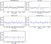 |
Fig. 1 EPIC/pn background-subtracted light curves for all observations of Kepler 63. The blue lines are the mean count rate (solid lines) obtained from the source-detection procedure, with the associated error (dashed lines). |
2.1 EPIC/pn light curves
The EPIC/pn light curves of Kepler-63 were extracted in the soft energy band of XMM-Newton (0.2–2.0 keV), employing the tools of SAS, evselect, and epiclccorr. All light curves were binned with a time bin size of 1000 s, with the exception of the observation of March 2020. In this case, the GTIs have a duration that is less than 1000 s and therefore a smaller bin size is more suitable. We chose 600 s.
Figure 1 shows the background-subtracted light curves of Kepler-63. In these plots, the solid blue lines represent the time-averaged count rates calculated with the source-detection procedure, and its uncertainties (dashed lines). These values are reported in Table 1.
We checked for short-term variability in each light curve, employing the software R and its package changepoint (Killick & Eckley 2014). This package allows the user to look for changes in the mean and variance in time-series data. The application of this method did not yield any significant short-term variability in our observations, that is, no flare-like events occurred during the X-ray monitoring of Kepler-63.
2.2 EPIC/pn spectra
The spectra of Kepler-63 were extracted for the whole energy band of XMM-Newton, i.e. 0.2–12.0 keV, and grouped with a minimum of 15 counts per bin, with the exception of the observation from March 2020. For this last observation, a grouping size of minimum 15 counts per bin would result in very few spectral bins, as it is the observation with the lowest photon statistics, and with a short exposure time. Therefore, only the spectrum of the observation of March 2020 was grouped choosing a minimum of 5 counts per bin. However, even with the reduced number of counts per bin, the spectrum of this observation does not have a sufficient number of bins to be properly fitted and was therefore excluded from the analysis.
Each of the other four spectra was analysed with the standard spectral software xspec (version 12.10; Arnaud 1996) and was fitted with the simplest thermal model, i.e. a one-temperature (1-T) APEC model, considering the energy range 0.3–2.0 keV1. The abundances Z are kept frozen during the fitting procedure, on a value equal to 0.3 Z⊙, which is typical for the corona of solar-like stars (Maggio et al. 2007). Tests for other values of abundances are explained in Sect. 2.2.1. The photoelectric absorption is not considered in the spectral model: although Kepler-63 is at a distance for which this effect plays a relevant role, i.e. at 200 pc, below 0.3 keV the uncertainties on the counts are too high to make the spectrum physically reliable.
The best-fitting values resulting from this procedure are reported in Table 2. The uncertainties on each best-fitting parameter are obtained with the error command of xspec, which calculates the confidence interval for the model parameters within a confidence level of 90%. The spectra of each observation, with the spectral model overplotted, are shown in Fig. B.1.
The observation from September 2014 and the one from August 2019 show sufficiently high statistics to be fitted with a 2-T APEC model. For these two spectra, the best-fitting parameters for the 2-T model are also shown in Table 2. The abundances are again frozen to the value of 0.3 Z⊙.
Best-fitting parameters for the X-ray spectra of Kepler-63.
2.2.1 Metal abundances
We carried out tests with the aim of constraining the coronal abundances for each observation. To this end, we adopted a 1-T APEC model in which the metal abundances were left free to vary during the fitting procedure. However, because of the low photon statistics shown by each spectrum, a statistically significant fit was not possible. Only the fit of the archival observation yielded a constrained value for Z, equal to 0.24 ± 0.07, with a reduced χ2 of 1.25 (with 25 d.o.f).
We additionally noticed that when considering a range of different values of metal abundances, each of them kept frozen in the fitting procedure, the statistics of the fit did not show significant differences. Thus, with the quality of the available data, we cannot constrain the coronal metal abundances. For thew subsequent analysis, we kept the metal abundances frozen to 0.3 Z⊙, as mentioned above.
2.2.2 Simultaneous fitting
We performed a simultaneous fit of all usable observations obtained in 2019 (three observations in total) in order to increase the signal-to-noise ratio (S/N). This allowed us to use a 2-T APEC model. The 2-T fit enables (1) a more detailed comparison to the observation from September 2014 and (2) a more meaningful investigation of Kepler-63 in the framework of the study “The Sun as an X-ray star” (see Sect. 3).
We carried out the simultaneous fit as described in Sect. 2.2. The results are shown in the bottom right panel of Fig. B.1 and reported in Table 2.
3 Modelling the corona of Kepler-63 in terms of solar magnetic structures
Here, we present our technique for indirectly identifying magnetic structures on the corona of Kepler-63. As explained in Sect. 1, the method is based on the study “The Sun as an X-ray star” and was previously applied to the old binary star HD 81809 (Favata et al. 2008; Orlando et al. 2017) and the young solarlike star ϵ Eridani (Coffaro et al. 2020). In Sect. 3.1, we present a summary of the study “The Sun as an X-ray star”, and then describe its application to the case of Kepler-63 (Sect. 3.2).
3.1 The solar emission measure distributions
In the study “The Sun as an X-ray star”, different types of magnetic structures observed with the Soft X-ray Telescope (SXT) on board the solar satellite Yohkoh on the corona of the Sun during the 22nd solar activity cycle were spatially and temporally analysed. The three kinds of structures that were identified in the X-ray images of the Sun are quiet regions (also termed background corona, BKCs), active regions (ARs), and cores of active regions (COs). For each of these structures, a distribution of emission measures as a function of temperature (EMD) was derived from the observations. In this way, for each phase of the solar cycle it was possible to identify the contribution of each type of magnetic structure to the total EMD.
The Yohkoh satellite also provided several images of solar flares on the corona, and eight flares were analysed over time, from their rise and throughout their decay (Reale et al. 2001). These flares range from Class C (relatively low-energy flares) to Class X (the most energetic ones observed on the Sun), and the corresponding flare EMDs were retrieved. Moreover, Yohkoh collected observations of flares with different filters, hard filters sensitive to plasma temperatures around and above 107 K, and soft filters for lower temperatures. The vast majority of the flares were observed with a pair of hard filters only; a few of them were observed also with a pair of soft filters, thus allowing a better reconstruction of the EMD at temperatures as low as 3 MK. One of these flares (a Class M flare, namely a flare of mid energy) was observed with two pairs of filters (soft and hard) and analysed by Reale et al. (2001). It was also possible to trace the temporal evolution of one AR and its corresponding CO from the rise to the decay (see Fig. 2 of Orlando et al. 2004).
In the final paper of “The Sun as an X-ray star” (Orlando et al. 2001), for each observed type of solar EMD, that is, BKCs, ARs, and COs, a corresponding synthetic spectrum was extracted using the response matrix of X-ray satellites that can observe stars. This way, Orlando et al. (2001) simulated solar coronal observations as if the Sun was observed by non-solar X-ray instruments.
3.2 The case of Kepler-63
With the aim of investigating whether and how the corona of young active stars can be described by magnetic structures similar to those observed in the solar corona, we applied the method presented in Sect. 3.1 to Kepler-63. The Sun is indeed the only star on which magnetic structures can be spatially and temporally resolved with current technology, and therefore the corona of the Sun is the only template that can be used for such investigations.
For applying the above study, we considered that at least two spectral components are needed in order to achieve a basic description of the temperature structure of the corona. However, the individual observations of the 2019 campaign are too poor for a 2-T fit, and therefore we fitted the three spectra jointly (see Sect. 2.2.2). We therefore have two epochs with spectral fits for Kepler-63 available: one representing the archival observation (from 2014) and one representing the average corona observed in 2019.
3.2.1 Choice of the appropriate magnetic structures
In the first step we aimed at finding the appropriate types of magnetic structures whose EMDs, scaled to the coronal metal abundance (i.e. 0.3 Z⊙) and the surface area of Kepler-63 (R★ = 0.91 R⊙; Sanchis-Ojeda et al. 2013), are suited to reproducing the X-ray luminosity (LX) and emission-measure-weighted thermal energies (kTav) observed during the XXMM-Newton monitoring campaign of the star. The kTav is calculated as
 (1)
(1)
where kTi and EMi (i = 1, 2) are the spectral components of the 2-T APEC model.
In Fig. 2 we show the EMDs derived from Yohkoh data for the different types of coronal structures: BKCs (yellow line), ARs (red line), and COs (green line). The figure also shows two EMDs for flaring regions: one derived from a sample of flares from Class C to X observed with Yohkoh/SXT using a pair of hard filters (Reale et al. 2001; solid black line) and the other one derived from flares of the sample from Class C to M (dashed black line), with the latter also analysed using a pair of soft filters in addition to the hard ones.
From Fig. 2 we see that the EMD per unit surface area of the solar BKCs and ARs is much lower than that of the COs, and therefore any percentage of these two structures would negligibly contribute to the total EMD. Covering part of the corona with BKCs and/or ARs implies less space left available for other magnetic structures that have a higher surface brightness and would better reproduce the X-ray luminosity of Kepler-63, which is at least two orders of magnitude higher than that of the Sun (log Lx Kep63 [erg s−1] ~ 29 versus log LX⊙ [erg s−1] ~ 27.3; Peres et al. 2000). We interpret this as a clear indication that Kepler-63 requires a high surface coverage with COs, meaning that the contribution of BKCs and ARs to the X-ray emission is negligible. Therefore, we do not consider the contribution of BKCs and ARs in the following.
For the case of ϵ Eridani, Coffaro et al. (2020) used the EMD obtained from the CO observed in 1996 by Orlando et al. (2004), which was time-averaged during its evolution (solid green line in Fig. 2), together with the contribution of the EMDs of FLs. These EMDs of COs and FLs were able to reproduce the X-ray luminosity of ϵ Eridani (log LX ϵEri [erg s−1] ~ 28). Because of the higher X-ray luminosity of Kepler-63 (log LX Kep63 [erg s−1] ~ 29), it is necessary to increase the percentage of surface coverage of COs and FLs in order to reach the observed X-ray emission level of the star. We therefore started to test the same scenario adopted for the case of ϵ Eridani, where the synthetic corona is covered with time-averaged COs and FLs, albeit assuming a greater percentage of them than in the case of ϵ Eridani. For the flaring contribution, we tested two different FL EMDs as we describe in Sects. 3.2.4 and 3.2.5. These two distributions are plotted in Fig. 2 as solid and dotted black lines respectively.
We took into account that the different classes of flares have different occurrence rates and therefore the flare filling factor depends on the flare energy (here approximated by peak flux, alias GOES class). To determine the average contribution of the different flare classes to the total EMD, we assumed that the differential frequency of the peak flux (Fpeak) of solar flares is described as  with index α = 1.57. This is the value calculated by Aschwanden & Parnell (2002) from Yohkoh observations of solar flares. The flare flux frequency distribution (FFD) is normalised to the peak flux of the flare with the lowest flux (a Class C flare in the case of the sample of flares considered here). The flare filling factors we derive with our modelling thus apply to a Class C5.8 flare, and filling factors for flares with other peak fluxes can be obtained by scaling from the power law (see Sect. 4.4). We note that the normalization of the FFD is degenerate with the filling factor of flares. If the normalization was made on a less energetic flare, the absolute values for the flare frequencies of the more energetic events would be lower, and a higher filling factor would be required to compensate for this.
After defining the appropriate classes of magnetic structures (here COs and FLs), a grid of EMDs was constructed where each grid point is distinguished from the others by a different fractional surface coverage with each class of magnetic structure.
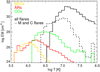 |
Fig. 2 Average EMDs per unit surface area for each type of magnetic structure observed with Yohkoh. The black lines are the two flaring EMDs tested within this work: a time-averaged distribution derived from a sample of eight flares from Class C to X observed with a pair of hard filters with Yohkoh (solid black line; Sect. 3.2.4) and a time-averaged distribution derived from the flares of Class C and M in the sample (dotted black line; Sect. 3.2.5); M flares were also observed with a pair of soft filters. |
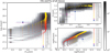 |
Fig. 3 X-ray luminosity as a function of emission-measure-weighted thermal energy kTav (left panel) and the two temperatures and emission measures (right panel). The circles represent the synthetic spectra extracted from EMDs that are composed of time-averaged COs varying from a coverage of 10–100% of the total coronal surface (change of colour shade) and FLs – from Class C to X time-averaged over their evolution – that vary from 0 to 4% of the area of the COs (change of symbol size). The best-fitting parameters of the observations of Kepler-63 are overplotted with the blue square (2014) and the magenta circle (2019). In the background, the occurrences of each best-fitting parameter – that is, simulated 1000 times for each combination of magnetic structures by introducing Poisson noise – are shown with the corresponding colour bar in log scale. |
3.2.2 Synthesis of the X-ray spectra
We extracted a synthetic XMM-Newton spectrum for each grid point, making use of the EPIC/pn response matrix and taking into account the distance of Kepler-63. In order to estimate uncertainties, 1000 spectra were generated for each grid point, and Poisson statistics were introduced in the extraction procedure for the synthesis of the spectra. Each of these 1000 spectra was then fitted in xspec with a 2-T APEC model, and with metal abundances frozen to 0.3 Z⊙, i.e. the same spectral model used to represent the observed spectra of Kepler-63. In this way, each grid point, i.e. each combination of magnetic structures, is not unequivocally represented by only two couples of kT s and EMs for the cold and hot components, but rather by a set of 1000 values for each of the four fit parameters drawn from a Poisson distribution. The four parameters (two kT s and two EMs) for each point of the final grid are calculated as the mean of the 1000 values obtained from the spectral analysis.
Furthermore, from analyzing the synthetic spectra, we obtained the X-ray luminosity as a function of the EM-weighted coronal temperature, calculated as in Eq. (1), and we performed a first visual comparison of these values with those calculated from the spectra of Kepler-63 in order to verify whether or not the chosen combination of magnetic structures can reproduce the observations. The left panel of Fig. 3 is an example of LX as a function of kTav, where the grid and the observations are compared. We discuss the details of such comparisons for different grids in Sects. 3.2.4 and 3.2.5.
As a final step, we performed a quantitative match between the temperatures and emission measures obtained from the analysis of the synthetic spectra with those retrieved from the observations, according to the approach described by Coffaro et al. (2020) and summarised in the following section.
3.2.3 Selection criterion
The match between synthetic and observed X-ray spectra of Kepler-63 was performed using a set of four equations, one for each of the four best-fitting parameters (kTi and EMi, with i = 1, 2), following Coffaro et al. (2020):
 (2)
(2)
where  are the parameters obtained from the spectral analysis of the observations of Kepler-63, and
  are the corresponding errors.
  are the best-fitting parameters of the synthetic spectra. The index j denotes the 1000 spectra, randomised with a Poisson distribution, generated for each k-th grid point2.
In Eq. (2), the parameter σ is the same for all four equations and determines the global confidence range of the match between observed and synthetic values. Thus, the criterion finds the set of best-fitting parameters for each of the 1000 sets (j) of spectra among all grid-points (k) within the smallest σ. At the end of the selection procedure, there are a total of 1000 best matches between one observation and the synthetic spectra, which correspond to a range of best-fitting combinations of young COs and FLs. From these 1000 representations, the unique best-matching combination of young COs and FLs was found from the median of the j selected values, associating the 10 and 90% quantile of these values as error.
3.2.4 Match with the standard flaring Sun
The first grid of EMDs and corresponding spectra that we tested is composed of time-averaged COs, varying from 10 to 100% coverage of the corona, and a distribution of FLs, time-averaged over their evolution and varying from 0 to 4% of the COs. The FL distribution was computed by considering a sample of flares from Class C to X observed with Yohkoh, from their rise to their decay phase (the average EMD per unit surface is shown in Fig. 2 as a black solid line), and taking into account the power-law FFD as explained in Sect. 3.2.1.
The plot of the X-ray luminosity as a function of the kTav calculated from this grid is shown in Fig. 3 on the left: each of the circles represents one point of the synthetic grid, that is one specific combination of magnetic structures. As the coverage fraction of COs increases on the corona, the X-ray luminosity increases while the EM-weighted thermal energy is less affected. Similarly, the greater the percentage of FLs, the higher the EM-weighted thermal energy, whereas the variation of X-ray luminosity is moderate3. This general behaviour of the grid is the same as that found for ϵ Eridani (Coffaro et al. 2020). In this figure, the best-fit parameters obtained from the spectral analysis of Kepler-63 (see Table 2) are also plotted.
The right panel in Fig. 3 shows the thermal energies and emission measures calculated from the grid and from the spectra of Kepler-63. The colour and size code of the plotting symbols are the same as in the left panel. We can see that an increase in the percentage of COs corresponds to an increase in EM1 and EM2 only, whereas the FLs influence both thermal energies and the EM2. The number of occurrences for each pair of the best-fitting parameters, obtained from the 1000 simulations of each k-th grid point, are shown in the background of each plot. The spread of these values provides an indication of the range of synthetic parameters compatible with the observations.
In Fig. 3, the LX – kTav plot shows that the chosen combination of magnetic structures can reproduce the EM-weighted thermal energy of Kepler-63, but the observed X-ray luminosity is not reached by the grid, that is, even a full surface coverage (100%) with COs and FLs does not produce enough LX at the observed values of kTav to explain the brightness of the corona of Kepler-63.
We note that the simulations presented above do not consider any extension of the corona above the chromosphere. In other words, the corona is assumed to have a thickness close to zero. However, the observations of the Sun show that the corona expands significantly above the chromosphere, with coronal magnetic loops of ARs extending up to 20–30% of the solar radius (DeForest 2007). It is therefore reasonable to consider an extension of the corona of Kepler-63 above the limb.
By assuming the same types of magnetic structures (time-averaged COs and FLs) with the same range of fractional coverage as before, we produced a grid of EMDs adopting a 30% larger radius for the corona of Kepler-63 to account for its extension above the chromosphere. The left panel in Fig. 4 shows LX as a function of kTav calculated from this grid. The coding of the plot follows that of Fig. 3. Here, the X-ray luminosity reproduces the observations of Kepler-63, although at the limit within the error bars. We therefore examined this model in more detail.
First, by adopting the selection criterion of Eq. (2), we obtained the EMDs that best match the observations; these are shown in Fig. 5. In these plots, the grey line is the total EMD that best matches the observations of Kepler-63, and the green and red lines are the EMDs of the COs and FLs that contribute to the total distribution at a given fraction coverage which is reported in the legend of the plots. The red and black symbols are the best-fitting parameters obtained from the spectral analysis of the actual spectra of Kepler-63 and the synthetic ones, respectively.
In Fig. 6 the ratio between the best-fitting parameters of the spectra of Kepler-63 and those of the best-matching synthetic spectra are plotted as circles. We note that the observations of 2019 (magenta circles) show better agreement with the selected models than the observation of 2014 (blue circles), which shows larger discrepancies in particular in terms of the ratios of the parameters of the first spectral component.
3.2.5 Match with the modified flaring Sun
To reduce the discrepancies seen in Figs. 4 and 5 between the best-fitting parameters of the models and those of the observations of Kepler-63, we need to change the components of the EMDs. As can be seen in Fig. 4 (right panel), a grid with lower kT2 and EM2 would better represent the data (especially for 2014). It is also clear in the plot that the COs reach the high X-ray luminosity of Kepler-63, and therefore this kind of structure is needed. We can therefore only modify the FL component. Furthermore, as we see from Fig. 4, we need smaller values of kT2, and so an FL distribution composed of mid-energetic flares appears more suited.
Among the solar flaring observations acquired with Yohkoh and presented by Reale et al. (2001), there are two Class M flares that were observed by the satellite with a pair of soft filters in addition to the pair of hard filters that are most frequently used for Yohkoh observations of flares. The soft filters yield an EMD that extends to lower temperatures, thus providing a more complete description of the EMD of flaring regions (see Reale et al. 2001, for more details). This is seen in Fig. 2 where the EMD that includes the soft-filter observations (dotted black line) extends to lower temperatures than the time-averaged EMD of all (hard-filter) flares in the sample observed with Yohkoh.
We therefore changed the FL distribution using the EMDs of Class M solar flares analysed with the two pairs of filters (soft and hard) and time-averaged across their evolution. Together with the Class M flares, we also considered the contribution of the Class С flare observed by Reale et al. (2001) to the EMD, as from the canonical flare frequency distribution (see Sect. 3.2.1) the number of Class С flares is higher than that of Class M events, and therefore the former cannot be excluded.
In this new simulation, the grid range of the coverage fraction of COs remains unchanged, and varies from 10 to 100%. The FLs are instead allowed to vary in a broader range of CO filling factor than before, namely 0–15%. This is motivated by the fact that the new FL component shows an EMD per unit surface area smaller than the flares from Class С to X used in the previous grid (see the dotted black line versus the solid one in Fig. 2). Moreover, the EMD of Class M flares covers a wider range of temperatures than the one of the time-averaged flares at different energies. This is due to the fact that the flaring distribution of Class M FLs was derived using both soft and hard filters, providing a contribution to the EMD at lower temperatures. Therefore, to reproduce the observed kTav, we needed to assume a higher percentage of FLs than in the previous case.
Starting from these EMDs, we extracted the corresponding synthetic spectra and analysed them as described above, using a 2-T APEC model. We then proceeded with the selection criterion explained in Sect. 3.2.3.
In Fig. 7, the plot of LX as a function of kTav (on the left) and the plots of the kTs and EMs (on the right) are shown. The coding of these plots is the same as for Fig. 3. Such a high percentage of FLs reproduces the X-ray luminosity without the need to account for the thickness of the corona of Kepler-635. In Fig. 8, the EMDs that best match the observations are shown. In Fig. 6, the ratios between the observed best-fitting parameters and the ones of the best-matching synthetic spectra for this test are shown as triangles. Here, the overall the ratios between the temperatures are closer to one than in the previous case, indicating that the replacement of the flaring EMD leads to better agreement between the observations and synthetic spectra. On the other hand, the EM values, and in particular those of the 2014 observation, have not changed significantly with respect to the previous combination of magnetic structures.
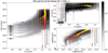 |
Fig. 4 X-ray luminosity as a function of emission-measure-weighted thermal energy kТav (left panel) and the kTs and EMs (right panel). The EMDs used for these grids assume the same magnetic structures and the same percentage coverage as in Fig. 3, with the difference that each EMD is scaled to a larger extension of the corona of Kepler-63, i.e. the stellar radius is set to be 30% larger. The coding of the plots follows Fig. 3. |
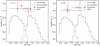 |
Fig. 5 EMDs constructed from solar magnetic regions that best match the observations of Kepler-63 (on the left: 2014; on the right: 2019). The contributions to the total EMD (grey line) are from time-averaged COs (green line) and FLs (red line) from Class С to X time-averaged over their evolution. The confidence level σ within which the models are selected is given in the upper left corner of each plot. The EMDs are scaled to a larger size of the corona of Kepler-63, i.e. 30% larger than its stellar radius. The red squares are the best-fitting parameters of the X-ray spectra of Kepler-63. The black circles are the best-fitting parameters retrieved from the best-matching synthetic spectra. The filling factor for the best-matching combination of magnetic structures is given in the legend. |
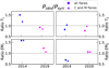 |
Fig. 6 Ratios between the best-fitting parameters of the spectra of Kepler-63 and the kT and EM values of the best-matching synthetic spectra4. The blue symbols are the ratios obtained from the comparison with the observation of 2014, whereas the magenta ones are obtained for the 2019 observations. The circles refer to those parameters calculated from the best-matching EMDs that have as flaring contribution the FLs from Class С to X time-averaged over their evolution (Sect. 3.2.4). The magenta triangles are instead calculated from the best-matching EMDs that include flares of Class С and M time-averaged over their evolution. (Sect. 3.2.5) |
4 Discussion
Kepler-63, a solar-like star with an age of only ~200 Myr, is the youngest star so far to be observed in X-rays with XMM-Newton with the goal of searching for a coronal magnetic cycle. Our X-ray monitoring campaign consisted of four snapshots of its corona, distributed between 2019 and 2020, thus spanning three-fifths of the photospheric cycle (Pcycl = 1.27 yr; Estrela & Valio 2016).
One additional observation was available in the XMM-Newton archive, dating back to 2014. Lalitha et al. (2018) analysed this observation using a 2-T APEC model, and obtained an X-ray luminosity log LX [erg s−1] = 29.00 ± 0.17 and an EM-weighted thermal energy kTav = 0.59 ± 0.07 keV. These values are in agreement with our analysis.
The spectral analysis of all available XMM-Newton observations, comprising the archival observation of 2014, yields a mean X-ray luminosity of log LX [erg s−1] = 29.03 ± 0.49, which corresponds to an X-ray surface flux of log FX,surf [erg cm−2 s−1] = 6.32 ± 0.05.
4.1 Search for an X-ray cycle
The photospheric cycle of Kepler-63 was revealed from observations with the Kepler telescope over 4 yr (from 2009 to 2013), during which the variation of stellar spots was monitored. The first observed minimum and maximum happened in August 2009 and March 2010, respectively (see Fig. 10 in Estrela & Valio 2016). We propagated the sinusoidal function representing the 1.27-yr photospheric cycle of Kepler-63 – that Estrela & Valio (2016) obtained from the Lomb-Scargle analysis of the number of spots seen in the photosphere6 – over time. We found that the maximum and minimum closest to our X-ray campaign were expected for the end of January 2019 and for mid-September 2019. In Fig. 9 we show the long-term X-ray light curve of Kepler-63 where the solid blue line is the folded sinusoidal function calculated by Estrela & Valio (2016) and the dotted line is our extrapolation of the photospheric cycle. The red symbols are the X-ray fluxes derived from our monitoring of Kepler-63. Clearly, the uncertainties of the X-ray flux in each XMM-Newton observation are larger than the changes of the flux between the observations. Therefore, we can only state that any potential X-ray cycle during our campaign in 2019-2020 had a minimum-to-maximum variation smaller than a factor 2.
4.2 Activity level and cycle amplitude of Kepler-63
In Fig. 10 we put Kepler-63 together with stars with known coronal cycle. It can be seen that Kepler-63 is the most active of them, that is, it presents the highest surface X-ray flux. Figure 10 shows the logarithm of the X-ray surface fluxes (FX,surf = LX/4πR★) as a function of the X-ray cycle amplitude (A = Lmax/Lmin) in log scale, defined as the variation of the X-ray luminosity between the maximum and minimum of the coronal cycle7. We note that there is a linear correlation between the log of these two quantities: as the X-ray activity level of the stars decreases (and, in turn, the stellar age increases), the amplitude of their coronal cycles increases. We interpret this result as being due to a decrease in the coverage of the stellar surface with magnetic structures as the star evolves. When the star is young, the massive presence of magnetic structures limits the variations of X-ray luminosity during the stellar cycle; when the star is old, the lower coverage of the stellar surface with coronal structures allows large variations of X-ray luminosity to be seen during the cycle. This scenario is consistent with the expectation from dynamo theory where the alternation of the α- and Ω-effect causes periodic changes in the number of magnetic structures, and their number is larger for faster rotators. As rotation rate drops with stellar age, our colour code in Fig. 10 can be taken as a code for rotation rate, and with Prot = 5 d, Kepler-63 is the fastest rotator in the sample.
According to the linear regression on the dataset in Fig. 10, the X-ray surface flux of the stars reaches a maximum value of log FX;surf [erg cm−2 s−1] ~ 6:13 when the stars have no activity cycle (i.e. when the amplitude log Lmax=Lmin = 0). However, this flux cannot be considered as an upper limit to the Xray flux that active stars can reach because X-ray observations have revealed a significant fraction of stars with fluxes up to log FX;surf [erg cm−2 s−1] ~ 7:5 (Schmitt 1997).We show through our modelling of Kepler-63 (summarised in Sect. 4.3) that the stellar corona is fully covered with magnetically active structures already at one order of magnitude smaller flux, and therefore such high values for FX;surf indicate not only that the coronae of these stars have a 100% filling factor but also that they must have flares of higher energy than the ones we infer to be present on Kepler-63. The presence of high-energy flares is a reasonable hypothesis, because for example pre-main sequence stars have flares with much greater energies (and X-ray fluxes) than solar flares (Getman & Feigelson 2021).
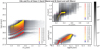 |
Fig. 7 X-ray luminosity as a function of emission-measure-weighted thermal energy kТav (left panel) and the two temperatures and emission measures (right panel). The EMDs used for generating these grids are composed of time-averaged COs covering from 10 to 100% of the total corona and FLs of Class С and Class M, time-averaged over their evolution and varying from 0 to 15% of the area of the COs. The Class M flares were also observed with Yohkoh with a pair of soft filters in addition to the pair of hard filters (used for the analysis of the Class С flare). The coding of the plots follows Fig. 3. |
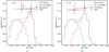 |
Fig. 8 EMDs constructed from solar magnetic regions that best match the observations of Kepler-63. The contributions to the total EMDs are from COs and FLs of Class С and Class M, time-averaged over their evolution. The confidence level σ within which the models are selected is given in the upper left corner of each plot. The coding of the plots follows Fig. 5. |
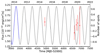 |
Fig. 9 Long-term X-ray light curve of Kepler-63. The red triangles are the X-ray fluxes calculated from the XMM-Newton observations, with their associated errors. The blue solid line is the sinuisodal function describing the photospheric cycle (1.27 yr) obtained by Estrela & Valio (2016). The dotted black line is our extrapolation of the sine curve. |
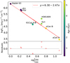 |
Fig. 10 X-ray surface flux of all stars with known X-ray cycles as a function of the cycle amplitude, i.e. the variation of LX between the maximum and the minimum of the activity cycle. Kepler-63 is included in the plot, although we detect no X-ray cycle. The colour bar denotes the ages of the stars. The dotted red line is the linear regression performed on the data set. The result of the fit is given in the legend of the plot, while the residuals of the procedure are reported in the bottom panel. |
4.3 Magnetic structures on the corona of Kepler-63 and implications for cycles
We quantitatively investigated whether or not the undetected X-ray cycle amplitude is linked to the massive presence of magnetic structures on the corona of Kepler-63 by applying a novel technique based on the study “The Sun as an X-ray star” (Sect. 3.1). This technique allows us to indirectly gain information on the magnetic structures that determine the X-ray emission level of Kepler-63. The method builds on the EMDs of the magnetic structures observed by the solar X-ray satellite Yohkoh on the corona of the Sun: BKCs, ARs, COs, and FLs. The EMDs can be built assuming that different percentages of these magnetic structures determine the total emission. From these EMDs, X-ray spectra of a pseudo-Sun (in the present case, Kepler-63) can then be synthesised as if they were collected with XMM-Newton.
In our previous application of this technique to ϵ Eridani (Coffaro et al. 2020), the high S/N of the observations enabled a very detailed description of the coronal temperature structure of the star in the form of a 3-T model fit to the EPIC/pn spectra. On the other hand, for the case of Kepler-63, we can analyse most of its EPIC/pn observations by employing a 1-T spectral model, as seen in Sect. 2.2. To increase the S/N, and thus enable the use of a 2-T spectral model to achieve a more detailed description of the corona of Kepler-63, it was necessary to reduce the X-ray monitoring campaign to only two observational epochs, one describing the corona in 2014 and the other describing its average behaviour during 2019. This was achieved by simultaneously analysing all observations acquired in that year.
We find that the coronal temperature structure of Kepler-63 is reproduced when we assume time-averaged COs together with a FL EMD. BKCs and ARs are neglected as they have a low surface brightness. Excluding BKCs and ARs does not imply that such regions are not present on the stellar corona. However, the high surface coverage of COs necessary to produce an X-ray luminosity as high as that observed leaves only a small percentage of the stellar surface available for BKCs and ARs. The low filling factor of these types of regions together with the fact that they are characterised by a much lower surface brightness in comparison with that of COs and FLs mean that the contribution of BKCs and ARs to the total X-ray emission of the star is negligible with respect to that of COs.
For the flaring contribution to the total EMD, we tested two scenarios: In the first one, we assumed that a distribution of flares from (GOES) Class С to Class X, from their rise to their decay, is present in the corona of Kepler-63, realigning its behaviour with that of a standard flaring Sun. In the second scenario, we assumed that only lower energetic flares, namely those from Class С (the least energetic flaring events of our sample) to Class M, are present. This was necessary because, as shown in Fig. 6, the first scenario cannot reproduce the X-ray temperatures observed in Kepler-63.
For the case of the standard flaring EMD, we examined the effect of scaling the simulated EMDs to two different sizes of the corona: in a first approach, we adopted the literature value for the radius of Kepler-63, neglecting the extension of its corona above the chromosphere. In a second test, we considered the possibility that the corona of Kepler-63 significantly extends above its surface, and in particular that the extension is 30% of the stellar radius (R★ = 0.91 R⊙). This hypothesis is motivated by solar observations, from which it is evident that the corona of the Sun is spread above the surface, expanding up to 20–30% of its radius (DeForest 2007).
Figures 5 and 8 show that, because of the large errors associated to each best-fitting parameter for both observations and synthetic spectra (black and red symbols), both tested scenarios (i.e. the EMDs with different flaring components and different sizes of the corona) can reproduce the spectra of Kepler-63. The parameter σ, which is defined in Eq. (2), has a value of ~ 1 when the selection criterion is run over the first scenario, i.e. the EMDs composed of all classes of FLs plus a 30% coronal extension. In the second tested case, namely the EMDs with Class C and M FLs and no extension of the corona, the value of σ is found to be equal to ~0.6. Thus, we choose this latter model as the preferred one. For this scenario, we find that the magnetic structures cover the whole corona, i.e. the filling factor is 100% for both X-ray epochs of Kepler-63 (Fig. 8). The complete coverage of the corona of Kepler-63 strengthens the hypothesis that the amplitude of an eventual X-ray cycle is significantly reduced by the massive presence of coronal structures in all phases of the cycle.
With the above simulation we can reproduce the observations of Kepler-63 without considering the thickness of the corona and therefore we underestimate the extension of the corona above the stellar surface. Therefore, the filling factors of the magnetic structures can be taken as upper limits. If we consider the corona to have an extent of 30% of the stellar radius covered with the same types of structures (i.e. Class C and M flares and COs), the surface coverage with magnetic structures is reduced by a factor of 1.7 and only ~60% of the corona is filled by COs and FLs. Most likely, the regions not covered with COs and FLs may be filled with BKCs and ARs. However, this has a negligible impact on the EMD and X-ray emission, as explained above. The lower coverage fraction of the extended corona would imply that a change in the X-ray luminosity by a factor of 2 is possible during the cycle of Kepler-63, as almost half of the corona would be free for new magnetic structures to rise and evolve during a potential cycle maximum. Although our data do not suggest the presence of an X-ray cycle, a factor 2 variation cannot be excluded given the large uncertainties on the individual flux measurements (see Fig. 9 and Sect. 4.1).
4.4 Nature of the flares on Kepler-63
Another intriguing characteristic we face is related to the nature of the magnetic structures we used for modelling the corona of Kepler-63. To best reproduce the coronal structure of Kepler-63, the hottest component of the total EMDs needs to be at a lower energy than the typical solar flare EMD (which indicatively has temperatures around 7–10 MK). To represent such energies, we made use of low- and mid-energy flares from Class C to M, but omitting the more energetic Class X events. As young solar-like stars show lower metallicity than the Sun, the radiative cooling is less efficient. This in turn implies that the evolution of flares is slowed down and the events are on average seen at lower temperatures. Thus, it is plausible that, overall, low- and mid-energetic flares are dominant on Kepler-63, and such a scenario is supported by our models.
We stress that we are exploring a quasi-stationary component of the corona of Kepler-63 resulting from the superposition of several unresolved flares. From the canonical power-law distribution, the frequency of higher energy flares (such as Class X flares) is expected to be lower than that of low-to-mid-energetic flares, and therefore they would not contribute significantly to the quasi-stationary component. High-energy flares may be revealed as short-term variability in the X-ray light curves. As a rough estimate, we can assume that a flare would have been detected in the light curve if it was 2δ above the mean count rate. Here δ is the standard deviation, and for Kepler-63 we find δ = 0.01 cts s−1. Using the rate-to-flux conversion factor obtained from the EPIC/pn spectral analysis (CF = 1.2 × 10⁻¹² erg cm−2 cts−1) such a 2δ event corresponds to a flux amplitude of 2.5 × 10⁻¹⁴ erg cm−2 s−1, and the corresponding peak flare flux at the surface of Kepler-63 is FX,surf,2δ = 2.3 × 10⁶ erg cm−2 s−1. The total surface flux of the quiescent X-ray emission of Kepler-63 (which includes the quasi-stationary flaring component) is 2.1 × 10⁶ erg cm−2 s−1. This means that a 2δ event has 1.1 times the total surface flux of the star; that is, only events that provide an X-ray flux that is higher than that of the rest of the star’s corona combined can be identified in the EPIC/pn light curve. Such events have 45 times the surface flux of an X9 Class flare. This estimate does not consider the different energy bands of XMM-Newton/EPIC and the GOES flare classification (see below for an estimate of the conversion). No clear flare signatures are seen in Fig. 1, but the strong variability between two subsequent bins of the light curve could, in principle, be caused by such high-energy flares. Judging from the light curves, the rate of such events would be one every 2–3 ksec with a duration of ~1 ksec (one bin) each. In this interpretation, the mean count rates indicated in Fig. 1 would not represent the quiescent activity level. We defer a more quantitative analysis of flare-detection thresholds to a future study. In the following, we estimate the number of Class X flares on Kepler-63 on the basis of the frequency distribution of flare energies.
The coronal filling factor for Class X flares can be estimated from the FFD power law. In our analysis, we normalised the FFD to the smallest Yohkoh flare which is of Class C5.8. With the power slope α = 1.57 we infer a flare frequency for Class X9 flares8 that is smaller than that of Class C5.8 flares by 7.2 × 10⁻⁴. Our modelling of the X-ray spectra of Kepler-63 in Sect. 3.2.5 yields a filling factor with FL of ~13.4% of the stellar surface. This number refers to Class C5.8 flares. Accordingly, the filling factor for Class X9 flares is f fX9 ~ 9.7 × 10⁻⁵. With a reasonable assumption on the coronal area covered by one such flare, we can estimate the number of Class X9 flares present on the surface of Kepler-63 at any time. We carry out the calculation assuming that the area covered by a Class X9 flare on the corona is Af = 3 × 1019 cm2. This value is directly derived from the Yohkoh images for the X9 flare of the sample which is our reference point (Reale et al. 2001). We then scale this result to the total surface area of Kepler-63. The number of Class X9 flares on Kepler-63, NX9, is then given by the ratio of the filling factor f fX9 and the fractional surface area of one such event,  . We find NX9 ~ 0.16. This means that bright flares are rare events on Kepler-63, justifying a posteriori the omission of Class X flares in our EMD modelling on timescales consistent with those of observations.
We note that several uncertainties contribute to this calculation of the flare number and energetics. In particular, the number of X9 Class flares depends strongly on the area covered by such an event. The Yohkoh X9 flare from Reale et al. (2001) was a so-called complex flare, characterised by an arcade of loops. The value for the flare area derived by Reale et al. (2001) for this event is consistent with the areas inferred by Aschwanden & Aschwanden (2008) for GOES Class M and Class X flares. Our above estimate for the flare number is therefore likely to be representative of solar flares in general.
A second uncertainty in our modelling is the slope of the FFD distribution for which we used the Yohkoh value, α = 1.57. If we instead assume a steeper FFD (α = 2.0, based on observations of stellar flares in the optical; see e.g. the summary by Ilin et al. 2021), the conditions are even more relaxed, yielding flare numbers that are lower by approximately a factor of 10.
Finally, as mentioned in Sect. 4.4, we are mixing numbers derived from different instruments. The flare classification is based on GOES 1–8 Å flux while our analysis uses data from the Yohkoh/SXT. Argiroffi et al. (2008) determined the scaling between the flare emission measures observed with these two instruments to be EMYohkoh ~ 0.5 • EMGOES. The factor two uncertainties obtained if a similar relation holds for the flux values of Yohkoh and GOES are clearly smaller than the uncertainties caused by the other assumptions described above.
In summary, a calculation based on the properties of a Class X9 flare observed with Yohkoh shows that the number of such bright flares present in the corona of Kepler-63 is negligible, which is consistent with the requirements from our “The Sun as an X-ray star” modelling of the X-ray spectrum and with the non-detection of such events in the X-ray light curve of the star. However, for other plausible flare parameters, a higher number of X9-type events can be obtained, and such a scenario cannot be excluded by the X-ray light curve, which has too low a S/N to distinguish individual Class X flares.
5 Conclusions and outlook
With our simulations and their comparison to the observed XMM-Newton spectra we identify the types of solar magnetic structures that best reproduce the coronal X-ray emission of Kepler-63. We find that modifications are required as to the presence and relative importance of the different magnetic features with respect to those that dominate the X-ray emission of the Sun. In an earlier, analogous study of another young solar-like star, ϵ Eridani (Coffaro et al. 2020), we also had to adapt the solar magnetic structures to be able to fit the observations of the stellar corona, but in different ways from what we require for Kepler-63. We conclude that stellar coronae have a variety of physical characteristics.
The non-detection of an X-ray cycle on Kepler-63 is compatible with the complete coverage of its corona with magnetic structures, as we derive from our modelling. The correlation between cycle amplitude and X-ray surface flux that we find for the sample of stars with X-ray cycles suggests a limiting X-ray brightness for stars that can sustain cycles of log FX,surf [erg cm−2 s−1] ~ 6.3, the value of Kepler-63. Stars with much higher values of X-ray surface flux than Kepler-63 are known (see e.g. Schmitt 1997), and we speculate that these stars must present higher energy flares in order to reach their observed X-ray radiation output.
The modelling is likely also affected by the quality of the observations, for example the S/N of the stellar X-ray spectra and the range of flares included in the Yohkoh EMDs. Future works should address these points by investigating additional stellar X-ray observations with the technique of “The Sun as an X-ray star” and by improving the statistics for solar flares at all relevant energies.
Acknowledgements
We thank the anonymous referee for the useful input that improved our final discussion. M.C. acknowledges financial support by the Bundesministerium für Wirtschaft und Energie through the Deutsches Zentrum für Luft- und Raumfahrt e.V. (DLR) under the grant FKZ 50 OR 2008. S.O. acknowledges financial contribution from the agreement ASI-INAF n.2018-16-HH.0. This work is based on observations obtained with XMM-Newton, an ESA science mission with instruments and contributions directly funded by ESA Member States and NASA.
Appendix A EPIC/pn light curve of the background detector
Here, the light curve of the background detector of the EPIC/pn for each observation of Kepler-63 is shown. In each plot, the red lines and red intervals denote the GTIs chosen in each light curve as explained in Sect. 2.
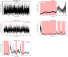 |
Fig. A.1 Light curves of the full-detector background of EPIC/pn. The red lines and the red intervals show where the GTIs were chosen. |
Appendix B Spectral analysis
The EPIC/pn spectra of Kepler-63 are shown in this section. The solid red line is the spectral model (APEC) used for fitting the observations. The bottom panels in each plot are the residuals of the fitting. For the observations of 2014, of August 2019, and the simultaneous fit of 2019 observations, a two-temperature spectral model is adopted. In all other cases, only one thermal component is used, with the exception of the observation of March 2020. As explained in Sect. 2.2, this latter observation suffers from low photon statistics, and it is not possible to carry out a meaningful fit. Values of the best-fitting parameters are found in Table 2.
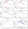 |
Fig. B.1 EPIC/pn spectra of Kepler-63. The solid line is the best-fitting spectral model. The bottom panels are the reduced χ2 residuals of the fitting. |
References
- Argiroffi, C., Peres, G., Orlando, S., & Reale, F. 2008, A&A, 488, 1069 [NASA ADS] [CrossRef] [EDP Sciences] [Google Scholar]
- Arnaud, K. A. 1996, ASP Conf. Ser., 101, 17 [Google Scholar]
- Aschwanden, M. J., & Aschwanden, P. D. 2008, ApJ, 674, 530 [NASA ADS] [CrossRef] [Google Scholar]
- Aschwanden, M. J., & Parnell, C. E. 2002, ApJ, 572, 1048 [NASA ADS] [CrossRef] [Google Scholar]
- Böhm-Vitense, E. 2007, ApJ, 657, 486 [CrossRef] [Google Scholar]
- Coffaro, M., Stelzer, B., Orlando, S., et al. 2020, A&A, 636, A49 [EDP Sciences] [Google Scholar]
- DeForest, C. E. 2007, ApJ, 661, 532 [NASA ADS] [CrossRef] [Google Scholar]
- de la Calle, I. 2019, Users Guide to the XMM-Newton Science Analysis System [Google Scholar]
- Estrela, R., & Valio, A. 2016, ApJ, 831, 57 [NASA ADS] [CrossRef] [Google Scholar]
- Favata, F., Micela, G., Orlando, S., et al. 2008, A&A, 490, 1121 [NASA ADS] [CrossRef] [EDP Sciences] [Google Scholar]
- Getman, K. V., & Feigelson, E. D. 2021, ApJ, 916, 32 [NASA ADS] [CrossRef] [Google Scholar]
- Hempelmann, A., Robrade, J., Schmitt, J. H. M. M., et al. 2006, A&A, 460, 261 [NASA ADS] [CrossRef] [EDP Sciences] [Google Scholar]
- Ilin, E., Poppenhäger, K., & Alvarado-Gómez, J. D. 2021, Astron. Nachr., submitted [arXiv:2112.09676] [Google Scholar]
- Killick, R., & Eckley, I. 2014, J. Stat. Softw., Articles, 58, 1 [Google Scholar]
- Lalitha, S., Schmitt, J. H. M. M., & Dash, S. 2018, MNRAS, 477, 808 [NASA ADS] [CrossRef] [Google Scholar]
- Maggio, A., Flaccomio, E., Favata, F., et al. 2007, ApJ, 660, 1462 [NASA ADS] [CrossRef] [Google Scholar]
- Netto, Y., & Valio, A. 2020, A&A, 635, A78 [NASA ADS] [CrossRef] [EDP Sciences] [Google Scholar]
- Orlando, S., Peres, G., & Reale, F. 2000, ApJ, 528, 524 [NASA ADS] [CrossRef] [Google Scholar]
- Orlando, S., Peres, G., & Reale, F. 2001, ApJ, 560, 499 [NASA ADS] [CrossRef] [Google Scholar]
- Orlando, S., Peres, G., & Reale, F. 2004, A&A, 424, 677 [NASA ADS] [CrossRef] [EDP Sciences] [Google Scholar]
- Orlando, S., Favata, F., Micela, G., et al. 2017, A&A, 605, A19 [NASA ADS] [CrossRef] [EDP Sciences] [Google Scholar]
- Peres, G., Orlando, S., Reale, F., Rosner, R., & Hudson, H. 2000, ApJ, 528, 537 [NASA ADS] [CrossRef] [Google Scholar]
- Reale, F., Peres, G., & Orlando, S. 2001, ApJ, 557, 906 [CrossRef] [Google Scholar]
- Robrade, J., Schmitt, J. H. M. M., & Favata, F. 2012, A&A, 543, A84 [NASA ADS] [CrossRef] [EDP Sciences] [Google Scholar]
- Sanchis-Ojeda, R., Winn, J. N., Marcy, G. W., et al. 2013, ApJ, 775, 54 [Google Scholar]
- Sanz-Forcada, J., Stelzer, B., & Metcalfe, T. S. 2013, A&A, 553, L6 [NASA ADS] [CrossRef] [EDP Sciences] [Google Scholar]
- Sanz-Forcada, J., Stelzer, B., Coffaro, M., Raetz, S., & Alvarado-Gómez, J. D. 2019, A&A, 631, A45 [NASA ADS] [CrossRef] [EDP Sciences] [Google Scholar]
- Schmitt, J. H. M. M. 1997, A&A, 318, 215 [NASA ADS] [Google Scholar]
- Silva, A. V. R. 2003, ApJ, 585, L147 [Google Scholar]
- Wilson, O. C. 1978, ApJ, 226, 379 [Google Scholar]
Beyond 2.0 keV the spectra are extremely noisy and the high uncertainties would compromise the goodness of the fit.
This trend of X-ray luminosity and EM-weighted thermal energy, induced by magnetic structures was reported for the Sun by Orlando et al. (2004).
The error bars are not taken into account as the calculated uncertainties are greater than the corresponding ratios.
We note that neglecting the thickness of the corona corresponds to deriving an upper limit to the surface coverage of COs and FLs; see discussion in Sect. 4.3.
The number of spots seen in the transit curve of Kepler-63 was scaled to the running mean over a range of five data points (i.e. five stellar spots) and to the residuals of a quadratic polynomial fit to the data. This implied that the final number of spots had non-interger and negative values (Estrela & Valio 2016).
The X-ray surface fluxes and the cycle amplitude of each star in the sample are calculated from the X-ray luminosity and the long-term light curves published in the literature (the Sun from Peres et al. 2000; α Centauri A and В and 61 Cygnus A and В from Robrade et al. 2012; HD81809 from Orlando et al. 2017; ι Horologii from Sanz-Forcada et al. 2019; ϵ Eridani from Coffaro et al. 2020).
We arbitrarily choose the X9 flare for our calculation since this is the largest flare in the Yohkoh sample (Reale et al. 2001); a more accurate treatment should take account of the continuous flare distribution.
All Tables
All Figures
|
Fig. 1 EPIC/pn background-subtracted light curves for all observations of Kepler 63. The blue lines are the mean count rate (solid lines) obtained from the source-detection procedure, with the associated error (dashed lines). |
| In the text | |
|
Fig. 2 Average EMDs per unit surface area for each type of magnetic structure observed with Yohkoh. The black lines are the two flaring EMDs tested within this work: a time-averaged distribution derived from a sample of eight flares from Class C to X observed with a pair of hard filters with Yohkoh (solid black line; Sect. 3.2.4) and a time-averaged distribution derived from the flares of Class C and M in the sample (dotted black line; Sect. 3.2.5); M flares were also observed with a pair of soft filters. |
| In the text | |
|
Fig. 3 X-ray luminosity as a function of emission-measure-weighted thermal energy kTav (left panel) and the two temperatures and emission measures (right panel). The circles represent the synthetic spectra extracted from EMDs that are composed of time-averaged COs varying from a coverage of 10–100% of the total coronal surface (change of colour shade) and FLs – from Class C to X time-averaged over their evolution – that vary from 0 to 4% of the area of the COs (change of symbol size). The best-fitting parameters of the observations of Kepler-63 are overplotted with the blue square (2014) and the magenta circle (2019). In the background, the occurrences of each best-fitting parameter – that is, simulated 1000 times for each combination of magnetic structures by introducing Poisson noise – are shown with the corresponding colour bar in log scale. |
| In the text | |
|
Fig. 4 X-ray luminosity as a function of emission-measure-weighted thermal energy kТav (left panel) and the kTs and EMs (right panel). The EMDs used for these grids assume the same magnetic structures and the same percentage coverage as in Fig. 3, with the difference that each EMD is scaled to a larger extension of the corona of Kepler-63, i.e. the stellar radius is set to be 30% larger. The coding of the plots follows Fig. 3. |
| In the text | |
|
Fig. 5 EMDs constructed from solar magnetic regions that best match the observations of Kepler-63 (on the left: 2014; on the right: 2019). The contributions to the total EMD (grey line) are from time-averaged COs (green line) and FLs (red line) from Class С to X time-averaged over their evolution. The confidence level σ within which the models are selected is given in the upper left corner of each plot. The EMDs are scaled to a larger size of the corona of Kepler-63, i.e. 30% larger than its stellar radius. The red squares are the best-fitting parameters of the X-ray spectra of Kepler-63. The black circles are the best-fitting parameters retrieved from the best-matching synthetic spectra. The filling factor for the best-matching combination of magnetic structures is given in the legend. |
| In the text | |
|
Fig. 6 Ratios between the best-fitting parameters of the spectra of Kepler-63 and the kT and EM values of the best-matching synthetic spectra4. The blue symbols are the ratios obtained from the comparison with the observation of 2014, whereas the magenta ones are obtained for the 2019 observations. The circles refer to those parameters calculated from the best-matching EMDs that have as flaring contribution the FLs from Class С to X time-averaged over their evolution (Sect. 3.2.4). The magenta triangles are instead calculated from the best-matching EMDs that include flares of Class С and M time-averaged over their evolution. (Sect. 3.2.5) |
| In the text | |
|
Fig. 7 X-ray luminosity as a function of emission-measure-weighted thermal energy kТav (left panel) and the two temperatures and emission measures (right panel). The EMDs used for generating these grids are composed of time-averaged COs covering from 10 to 100% of the total corona and FLs of Class С and Class M, time-averaged over their evolution and varying from 0 to 15% of the area of the COs. The Class M flares were also observed with Yohkoh with a pair of soft filters in addition to the pair of hard filters (used for the analysis of the Class С flare). The coding of the plots follows Fig. 3. |
| In the text | |
|
Fig. 8 EMDs constructed from solar magnetic regions that best match the observations of Kepler-63. The contributions to the total EMDs are from COs and FLs of Class С and Class M, time-averaged over their evolution. The confidence level σ within which the models are selected is given in the upper left corner of each plot. The coding of the plots follows Fig. 5. |
| In the text | |
|
Fig. 9 Long-term X-ray light curve of Kepler-63. The red triangles are the X-ray fluxes calculated from the XMM-Newton observations, with their associated errors. The blue solid line is the sinuisodal function describing the photospheric cycle (1.27 yr) obtained by Estrela & Valio (2016). The dotted black line is our extrapolation of the sine curve. |
| In the text | |
|
Fig. 10 X-ray surface flux of all stars with known X-ray cycles as a function of the cycle amplitude, i.e. the variation of LX between the maximum and the minimum of the activity cycle. Kepler-63 is included in the plot, although we detect no X-ray cycle. The colour bar denotes the ages of the stars. The dotted red line is the linear regression performed on the data set. The result of the fit is given in the legend of the plot, while the residuals of the procedure are reported in the bottom panel. |
| In the text | |
|
Fig. A.1 Light curves of the full-detector background of EPIC/pn. The red lines and the red intervals show where the GTIs were chosen. |
| In the text | |
|
Fig. B.1 EPIC/pn spectra of Kepler-63. The solid line is the best-fitting spectral model. The bottom panels are the reduced χ2 residuals of the fitting. |
| In the text | |
Current usage metrics show cumulative count of Article Views (full-text article views including HTML views, PDF and ePub downloads, according to the available data) and Abstracts Views on Vision4Press platform.
Data correspond to usage on the plateform after 2015. The current usage metrics is available 48-96 hours after online publication and is updated daily on week days.
Initial download of the metrics may take a while.