| Issue |
A&A
Volume 661, May 2022
The Early Data Release of eROSITA and Mikhail Pavlinsky ART-XC on the SRG mission
|
|
|---|---|---|
| Article Number | A13 | |
| Number of page(s) | 15 | |
| Section | Cosmology (including clusters of galaxies) | |
| DOI | https://doi.org/10.1051/0004-6361/202141211 | |
| Published online | 18 May 2022 | |
The eROSITA Final Equatorial-Depth Survey (eFEDS)
LOFAR view of brightest cluster galaxies and AGN feedback
1
Hamburger Sternwarte, Universität Hamburg,
Gojenbergsweg 112,
21029
Hamburg, Germany
e-mail: thomas.pasini@hs.uni-hamburg.de
2
Max Planck Institute for Extraterrestrial Physics,
Giessenbachstrasse 1,
85748
Garching, Germany
3
Faculty of Physics, Ludwig-Maximilians-Universität,
Scheinerstr. 1,
81679
Munich, Germany
4
ASTRON, The Netherlands Institute for Radio Astronomy,
Postbus 2,
7990 AA
Dwingeloo, The Netherlands
5
Leiden Observatory, Leiden University,
PO Box 9513,
2300 RA
Leiden, The Netherlands
6
Centre for Astrophysics Research, School of Physics, Astronomy and Mathematics, University of Hertfordshire,
College Lane,
Hatfield
AL10 9AB, UK
7
IASF–Milano, INAF,
Via A. Corti 12,
20133
Milano, Italy
8
INAF–Istituto di Radioastronomia,
via P. Gobetti 101,
40129
Bologna, Italy
9
Argelander-Institut für Astronomie (AIfA), Universität Bonn,
Auf dem Hügel 71,
53121
Bonn, Germany
Received:
29
April
2021
Accepted:
24
June
2021
Context. During the performance verification phase of the Spectrum-Roentgen-Gamma eROSITA telescope, the eROSITA Final Equatorial-Depth Survey (eFEDS) was carried out. It covers a 140 deg2 field located at 126° < RA < 146° and–3° < Dec < + 6° with a nominal unvignetted exposure over the field of 2.2 ks. Five hundred and forty-two candidate clusters and groups were detected in this field, down to a flux limit FX ~ 10–14 erg s–1 cm–2 in the 0.5–2 keV band.
Aims. In order to understand radio-mode feedback in galaxy clusters, we study the radio emission of brightest cluster galaxies (BCGs) of eFEDS clusters and groups, and we relate it to the X-ray properties of the host cluster.
Methods. Using LOFAR, we identified 227 radio galaxies hosted in the BCGs of the 542 galaxy clusters and groups detected in eFEDS. We treated non-detections as radio upper limits. We analysed the properties of radio galaxies, such as redshift and luminosity distribution, offset from the cluster centre, largest linear size, and radio power. We studied their relation to the intracluster medium of the host cluster.
Results. We find that BCGs with radio-loud active galactic nucleus (AGN) are more likely to lie close to the cluster centre than radioquiet BCGs. There is a clear relation between the cluster X-ray luminosity and the 144 MHz radio power of the BCG. Statistical tests indicate that this correlation is not produced by biases or selection effects in the radio band. We see no apparent link between largest linear size of the radio galaxy and the central density in the host cluster. Converting the radio luminosity into kinetic luminosity, we find that radiative losses of the intracluster medium are in an overall balance with the heating provided by the central AGN. Finally, we tentatively classify our objects into disturbed and relaxed based on different morphological parameters, and we show that the link between the AGN and the ICM apparently holds for both subsamples, regardless of the dynamical state of the cluster.
Key words: galaxies: clusters: general / radio continuum: galaxies / X-rays: galaxies: clusters / galaxies: groups: general / galaxies: clusters: intracluster medium
© ESO 2022
1 Introduction
Radio galaxies that sit at the centres of galaxy clusters and galaxy groups play an important role in regulating the temperature of the intra-cluster medium (ICM) and intra-group medium (IGrM). Radio-loud active galactic nuclei (AGN) are usually hosted by brightest cluster galaxies (BCG) and they quench the cooling of the hot (~107 K) ICM through mechanical feedback (see e.g. reviews by McNamara & Nulsen 2012; Gitti et al. 2012). Effects of AGN feedback are manifested in the form of X-ray cavities and ripples in the cluster atmosphere (e.g. McNamara et al. 2000; Bîrzan et al. 2004; Fabian et al. 2006; Markevitch & Vikhlinin 2007; Gastaldello et al. 2009). Consequences are also observed in the thermodynamical properties of the ICM, such as the gas entropy distribution (e.g. Cavagnolo et al. 2009) or in the transport of high-metallicity gas from the cluster centre to the outskirts (e.g. Liu et al. 2019). This type of feedback is generally positive, in the sense that when the radiative losses of the ICM increase, the AGN counteracts this by heating the ICM. The more gas cools and fuels the super-massive black hole (SMBH) at the centre of the BCG, the higher the energy output that is able to quench the ICM radiative losses and establish what is commonly known as the AGN feedback loop (see the review from Gaspari et al. 2020). AGN feedback has been observed in systems ranging from isolated elliptical galaxies (Croton et al. 2006; Sijacki et al. 2015; O’Sullivan et al. 2011a) to massive clusters where it prevents the formation of cooling flows (McDonald et al. 2019; Ehlert et al. 2011; Pasini et al. 2021b). Most of the AGN associated with BCGs are in the so-called radio-or maintenance-mode (to distinguish it from the radiatively dominated quasar-mode feedback), where the accretion rate is modest and the feedback is mediated via mechanical work from powerful jets. A scaling relation between cavity power and radio luminosity, spanning over seven orders of magnitude in radio and jet power, has been observed in nearby systems (Bîrzan et al. 2004, 2008; Merloni & Heinz 2007; Cavagnolo et al. 2010; O’Sullivan et al. 2011b; Heckman & Best 2014).
It has been pointed out that AGN feedback may operate differently in galaxy groups, where the gravitational potential is shallower (Sun 2012). Here, less energetic AGN than in clusters can have a larger impact on the IGrM (Giodini et al. 2010) because outbursts are also capable of expelling cool gas from the central region (Alexander et al. 2010; Morganti et al. 2013). As a result, AGN feedback may break the self-similarity between galaxy clusters and groups, especially in terms of their baryonic properties (Jetha et al. 2007). Hence, galaxy groups may be particularly interesting to study AGN feedback because their different environment should be reflected in the properties of the central AGN (e.g. Giacintucci et al. 2011).
Von Der Linden et al. (2007) found that brightest group galaxies (BGGs) and BCGs lie on a different fundamental plane in terms of velocity dispersion, effective radius, and average surface brightness and have experienced star formation for a shorter time than non-BCGs1. In the companion paper by Best et al. (2007), they also argued that BCGs are more likely to host radio- loud AGN than satellites of the same mass (cluster-hosted and not), but are less likely to host an optical AGN. These differences are particularly pertinent for BGGs. Main et al. (2017) studied the relation between AGN feedback and central (at 0.004R500) cooling time in a sample of 45 galaxy clusters. They reported a clear correlation between AGN power, halo mass, and X-ray luminosity in clusters with a central cooling time of <1 Gyr.
X-ray observations of galaxy groups are more difficult than for galaxy clusters because groups have lower surface brightnesses and emit at lower temperatures that are outside of the sweet spot of most X-ray observatories (see e.g. Willis et al. 2005). Some notable work on groups has been reported, however. Lovisari et al. (2015) presented scaling relations in the group regime, and Johnson et al. (2009) and O’Sullivan et al. (2017) classified their samples of groups into cool-core and non-coolcore. Kolokythas et al. (2018) focused on central radio galaxies in the so-called Complete Local Volume Group Sample (CLoGS) and found that ~ 92% of groups in their high-richness sample (26 objects) have dominant galaxies (BGGs) hosting radio sources. They also argued that radio galaxies showing jets are more common in bright groups, while radio non-detections are mostly found in X-ray faint systems. In the CLoGS low-richness sample (27 objects) studied in Kolokythas et al. (2019), the same authors report a radio detection rate of ~82% in the luminosity range 1020–1025 WHz–1 at 235MHz. Malarecki et al. (2015) proposed that the lower densities in the IGrM compared to the ICM allow the lobes of group radio galaxies to expand to large distances. Werner et al. (2014) used far-infrared (FIR), optical, and X-ray data to study eight nearby giant elliptical galaxies, all central members of relatively low-mass groups. The authors found evidence that cold gas in these centrals galaxies is produced mostly by cooling from the hot phase and that this cool gas fuels outbursts of the AGN. Dunn et al. (2010) investigated a statistically complete sample of 18 nearby massive galaxies with X-ray and radio coverage and reported that 10 of them exhibit extended radio emission, with 9 also showing indications of interplay with the surrounding hot gas.
Mittal et al. (2009) determined that all cool-core clusters in a complete sample of ~60 clusters show a central radio galaxy, while only half of the non-cool core clusters have one. Interestingly, when this study was extended to galaxy groups, the trend became much weaker (Bharadwaj et al. 2014, 2015). A similar result was recently discussed in Pasini et al. (2020) (hereafter P20). In this paper, the authors studied a sample of 247 X-ray detected galaxy groups in the COSMOS field, matching them to radio galaxies detected in the VLA-COSMOS Deep Survey (Schinnerer et al. 2010) and in the COSMOS MeerKAT survey (MIGHTEE, Jarvis et al. 2016). They found that more than 70% of their radio galaxies are not hosted in BGGs, while in clusters, ~85% of the central radio galaxies are associated with BCGs. They also discussed a correlation between the X-ray luminosity of groups and the radio power from the central radio galaxy because more massive groups seem to host more powerful sources. Pasini et al. (2021a) recently showed that in their sample of groups, BGGs showing powerful radio emission are always found within 0.2 Rvir ~ 0.3 R200 from the centre.
The extended ROentgen Survey with an Imaging Telescope Array (eROSITA) on board the Spectrum-Roentgen-Gamma (SrG) mission (Predehl et al. 2021) was launched on July 13, 2019. The large effective area (1365 cm2 at 1 keV), large field of view (FoV, 1 deg diameter), good spatial resolution (half-energy width of 26″ averaged over the FoV at 1.49 keV, 16″ on-axis) and spectral resolution (~80 eV full width at half maximum at 1 keV) of eROSITA allow unique survey science capabilities by scanning large areas of the X-ray sky quickly and efficiently (Merloni et al. 2012). Thus, eROSITA is detecting a large number of previously undetected groups and clusters, most of them with low surface brightnesses and at low redshifts, even though the confirmation of these groups in the optical is challenging for z < 0.1-0.2.
In this work, we exploit the results of the eROSITA Final Equatorial-Depth Survey (eFEDS), a mini-survey designed to demonstrate the science capabilities of eROSITA. We study the radio galaxies observed in cluster centres at a frequency of 144 MHz by the LOw Frequency ARray (LOFAR, van Haarlem et al. 2013) in order to investigate their relation to their host clusters. This paper is structured as follows: in Sect. 2 we give a detailed description of how we built the sample. In Sect. 3, we show the results, compare them to previous work, and analyse the implications for AGN feedback. Finally, in Sect. 4 we summarise our results. Throughout this paper, we assume a standard ΛCDM cosmology with H0 = 70 kms–1 Mpc–1, ΩΛ = 0.7 and Ωm = 1−ΩΛ = 0.3.
2 Sample
2.1 eROSITA observation of eFEDS and the cluster catalogue
eFEDS covers a 140 deg2 field located in an equatorial region, with RA from ~126 to ~ 146 deg, and declination from ~−3 to ~6deg. This field was uniformly scanned by eROSITA during the Performance Verification phase, resulting in a nominal exposure of about 2.2 ks (unvignetted) over the field, which is similar in depth to the final exposure that will be reached in four years in equatorial fields in the eROSITA all-sky survey (Liu et al. 2022).
The eFEDS data were acquired by eROSITA over four days, between November 4 and 7, 2019. These data were processed by the eROSITA Standard Analysis Software System (eSASS, Brunner et al. 2022). We refer to Ghirardini et al. (2022, hereafter G22) for further details on the data processing. The source detection was performed using the tool erbox in eSASS on the merged 0.2–2.3 keV image of all seven eROSITA telescope modules (TMs). erbox is a modified sliding-box algorithm that searches for sources in the input image that are brighter than the expected background fluctuation at a given image position. For each candidate source, the detection likelihood and the extent likelihood are determined by fitting the image with the source model, which is a β-model convolved with the calibrated point spread function (PSF). Sources for which the extension is too broad to be fitted by the PSF have a higher extent likelihood. For further details on the source detection procedure, we refer to Brunner et al. (2022). We detect 542 candidate clusters over the full field (Liu et al. 2022). This corresponds to a source density of ~4 clusters per square degree at the equatorial depth. Photometric redshifts are obtained through the multi-component matched filter (MCMF) cluster confirmation tool (Klein et al. 2018). Optical data from the Hyper Suprime-Cam Subaru Strategic Program (HSC-SSP, Aihara et al. 2018) and from the DESI Legacy Survey (LS, Dey et al. 2019) were exploited. We refer to Klein et al. (2022) and Liu et al. (2022) for further details. Spectroscopic redshifts derived from 2MRS (Huchra et al. 2012), SDSS (Blanton et al. 2017), or GAMA (Driver et al. 2009) were used when available (296 out of 542 clusters). For each cluster, a massive red-sequence galaxy near the X-ray emission peak was selected as the BCG, following Klein et al. (2022).
The sample of clusters can be expected to be contaminated by spurious sources or by misclassified AGN at a level of ~19.7% (see Liu et al. 2022). Cluster contamination is therefore taken into account through the parameter fcont;i (Klein et al. 2019), which is defined as
 (1)
(1)
where frand,z is the richness distribution of random positions at the cluster candidate redshift zi, fobs(λ, zi:) is the richness distribution of true candidates, and λi is the richness of the cluster candidate. The estimator fcont;i is correlated with the probability of a source being a chance superposition. Applying a given cut to this parameter allowed us to reduce the initial contamination of the cluster sample. When independence of contaminants in the X-ray sample is assumed, the fractional contamination of the sample is simply the product of the initial fractional contamination of the X-ray sample and the applied cut in fcont For example, applying a cut in fcont,i < 0.3 results in a sample of about 88% (477 out of 542) of the eFEDS extended sources that are confirmed as galaxy clusters. When an initial contamination of the X-ray sample of 20% is assumed (Klein et al. 2022), this fcont selected sample is expected to contain ~6% contamination. Subsequent tests described in Klein et al. (2022) confirmed the expected amount of contamination to be 6 ± 3%. For more details about the X-ray catalog, we refer to Liu et al. (2022), while further details on the optical confirmation and contamination can be found in Klein et al. (2022).
2.2 LOFAR observations of eFEDS and the radio source catalogue
The eFEDS field was observed with the LOFAR high band antennae (HBA) for a total of 184 h (including simultaneous observations by two LOFAR pointings) between February 24, 2016, and May 27, 2020, by projects LC13_029 (100 h), LT5_007 (32 h), LT10_010 (44 h), and LT14_004 (8 h). The eFEDS field is entirely covered by six pointings of LC13_029 that are separated by 2.7° in a row. The LT5_007 observations that are centred on the GAMA 09 field cover the central region of the eFEDS field with four pointings separated by 2.4°. LT10_010 and LT14_004, as part of the LOFAR Two-meter Sky Survey (LoTSS; Shimwell et al. 2017, 2019), are positioned on the LoTSS grid where pointings are typically 2.58° apart. We present a layout of the LOFAR observations of the eFEDS field in Fig. 1. The setup for all observations is described in detail in Shimwell et al. (2017, 2019). The observing frequency is from 120 MHz to 187 MHz, but we removed the data above 168 MHz where the signal is highly contaminated by RFI. Each pointing was performed by multiple chunks of 2 or 4 h when the field was at high elevation (i.e. an average elevation of 35°). Bright radio sources 3C 196 and/or 3C 295 were observed for 10 min each before and after the observations of the target fields and were used as primary calibrators. Details of the observations are given in Table 1.
We adopted the standard calibration procedure that has been developed for LoTSS (Shimwell et al. 2017, 2019). The calibration aims to correct for the direction-independent and direction-dependent effects (e.g. ionosphere and beam model errors), which need to be corrected for high-fidelity imaging with the LOFAR HBA. The data for each pointing were separately processed with PREFACTOR2 (van Weeren et al. 2016; Williams et al. 2016; de Gasperin et al. 2019) and DDF-pipeline3 (Tasse 2014a,b; Smirnov & Tasse 2015; Tasse et al. 2018, 2021). In detail, the processing was identical to that described by Tasse et al. (2021), with one exception: in order to deal with the effect of sources that lie outside the target 8 × 8 degree field, but are still covered by the very N–S elongated LOFAR primary beam, the first step of the pipeline for each image was to make a very large (27 × 27 degree) image of the whole primary beam and subtract sources detected by DDFacet that appeared in this image, but lay outside the target field.
The pipeline produces high-resolution (<9″) images for each pointing with an rms noise of ≈ 170 μJy beam−1 in the pointing centre and ≈ 335 μJy beam−1 in the regions 2.5° from the pointing centres. Given the large LOFAR station beam (i.e. FWHM of 4° in an E–W direction at the central frequency of 144 MHz), the separation of 2.4–2.7° between the pointings leads to a significant overlap between the images. To increase the fidelity of the images, we convolved the images to a common resolution of 8″ × 9″ and made a mosaic of the entire eFEDS field in the manner described by Shimwell et al. (2019) by reprojecting each image onto a 50 000 × 27 000 pixel image with 1.5″ pixels centred on RA = 9 h, Dec = 1° and then combining the reprojected images weighting by the local image noise at each pixel, taking the primary station beam into account. No astrometric blanking was carried out in the mosaicing, and each image was corrected before mosaicing to the flux scale of Roger et al. (1973) in the manner described by Hardcastle et al. (2021). The noise in the resulting mosaic is non-uniform, but reduces to ≈ 135 μJy beam−1 in the central parts of the image.
To produce a catalog of radio sources, we performed source detection on the high-resolution (8″ × 9″) mosaic of the eFEDS field with the Python Blob Detector and Source Finder (PyBDSF4; Mohan & Rafferty 2015). Sources were detected with a peak detection threshold of 5σ (thresh_pix = 5) and an island threshold of 4σ (thresh_isl = 4) that limits the boundary for the source fitting. Here, the local noise rms, σ, was calculated using a box of (150 × 150) pixels2 that slides across the mosaic with a step of 15 pixels. Around bright sources, typically compact, where the pixel values are higher than 150σ (adaptive_thresh = 150), we used a smaller box of (60 × 60) pixels2 and a sliding step of 15 pixels. The smaller box is more accurate for the estimate of the high noise rms around bright sources. The source detection produces a catalog of 45 207 sources, most of which (99.6%) have 144 MHz flux densities below 1 Jy.
The mosaic that is made with the standard procedure described above typically has a flux density uncertainty of 10%. However, to further check the flux scale in the eFEDS mosaic, we compared the integrated flux densities of the LOFAR detected sources with those in the TGSS-ADR1 (TIFR GMRT Sky Survey–Alternative Data Release 1, Intema et al. 2017) 150 MHz data, which have a similar central frequency. The LOFAR mosaic was smoothed to the resolution of the TGSS- ADR1 (i.e. 25″) and regridded to match the spatial dimensions of the TGSS-ADR1 image. Radio sources in the LOFAR and TGSS-ADR1 25″ images are detected with PyBDSF in an identical manner as for the LOFAR 8″×9″ mosaic above. There are 4585 sources detected with both LOFAR and TGSS-ADR1 observations. Sixty percent of these sources (i.e. 2695) were modeled with a single Gaussian and were used for the flux scale comparison. Because the observing frequencies for the LOFAR and TGSS-ADR1 data are different, we rescaled the flux densities of the TGSS-ADR1 sources to match those at the frequency of the LOFAR data (144 MHz) by assuming a common spectral index of 0.8 (see Sect. 2.3 for a definition). We performed a linear fit to the LOFAR and TGSS-ADR1 scaled flux densities, weighting by the LOFAR flux densities, and obtained a relation log10 (SLOFAR) = 0.92 × log10(STGSS-ADR1;scaled) + 0.03 (Jy). The integrated flux densities of the radio sources in the LOFAR catalog are ~10% higher than those in the TGSS-ADR1 catalogue. We assumed an uncertainty of 20% for the integrated flux densities of the LOFAR detected sources. In Fig. 2, we present a scatter plot of the flux densities of the LOFAR and TGSS-ADR1 detected sources. The LOFAR detected sources, especially the faint ones, have higher flux densities than those found with the TGSS-ADR1 observations.
Following Shimwell et al. (2019), we checked the astrometry of the sources detected with PyBDSF in the LOFAR 8″ × 9″ mosaic by comparing their locations with those of their FIRST 1.4 GHz counterparts. We used the FIRST survey because of its high astrometric accuracy of 0.1″ compared to the absolute radio reference frame (White et al. 1997) and the comparable spatial resolution of both surveys (i.e. 5″ × 5″ for FIrSt and 8″ × 9″ for LOFAR). We cross-matched the sources within a radius of 9″ in the LOFAR and FIRST catalogues and found 10709 sources in common, of which 6601 are singleGaussian LOFAR sources. We calculated the offsets in RA and Dec for these single-Gaussian sources and present them in Fig. 2. The histograms of the RA and Dec offsets are fitted with a Gaussian whose location and standard deviation are defined as the systematic offsets and total astrometric uncertainty. There are systematic offsets of 0.13″ and 0.04″ in RA and Dec, respectively. The standard deviations of the offsets in RA and Dec are 0.70″ and 0.82″, respectively. When this is compared to the offsets of FIRST and LoTSS sources (Shimwell et al. 2019), our results on the RA and Dec offsets are a factor of two to seven higher, and the standard deviations are a factor of two to three higher. These are likely due to the lower declination of the eFEDS field compared with the declination of ~50° of the LoTSS-DR1 field, which results in a larger elongated beam and slightly more disturbed ionospheric conditions. However, the uncertainties are well within the resolution of the LOFAR observations (i.e. 8″ × 9″).
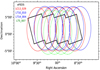 |
Fig. 1 LOFAR observations of the eFEDS field, shown in the black region. The elliptical lines show the LOFAR pointing locations in the projects LC13_029 (red), LT5_007 (green), LT10_010 (blue), and LT14_004 (blue). The major and minor axes of the ellipse (i.e. 4.0° and 6.7°) are the FWHM of the LOFAR station beam along the RA and Dec axes, respectively. |
LOFAR HBA observations of the eFEDS field.
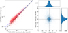 |
Fig. 2 Left: scatter plot between the TGSS-ADR1 (scaled) and LOFAR flux densities for single-Gaussian sources. The dashed blue line is the best fit of the LOFAR and TGSS-ADR1 (scaled) flux densities, log10 (SlOfar) = 0.92 × log10 (STGSS-ADRI;scaled) + 0.03 (Jy). The solid black line is a diagonal line with slope 1. Right: RA and Dec offsets for the LOFAR and FIRST detected single-Gaussian sources. The histograms of the offsets, including the best-fit Gaussian dashed lines, are plotted in the top and right panels. The ellipse shows the peak location (i.e. 0.13″ to the left and 0.04″ to the top of the centre point) and the FWHM (i.e. 0.70″ and 0.82″ in RA and Dec) of the Gaussian functions that are obtained from the fitting of the RA and Dec offset histograms. |
2.3 Sample construction and properties
The catalogue of radio sources was cross-matched with the BCG positions (see Sect. 2.1) by setting a sky threshold ~3θ, with θ being the synthesised beam of the interferometric radio observation. The results were then manually inspected to check for the presence of false positives (i.e. radio sources incorrectly associated with an optical BCG) or false negatives (i.e. radio emission lying at more than 30 from the BCG, but with an obvious association to it). We find no incorrect BCG-radio association, while two clusters were initially mistakenly classified as non-detections. To limit contamination, we applied the same cut fcont,i < 0.3 as discussed in Sect. 2.1. According to Eq. (1), this implies that we statistically allowed for 6% contamination. This value, albeit conservative, produces a relatively small impact on our results.
The final catalog contains a total of 227 clusters, with only ~1% (3 out of 230) of objects lost to contamination. This is consistent with our expectations because the cut we applied should result in a cluster catalogue that is ~99% complete (see Klein et al. 2022; Liu et al. 2022). Out of the parent sample of 542 X-ray clusters, 312 did not match any of LOFAR radio sources. After applying the same contamination criteria, we were left with 248 clusters without detected radio emission, which is a loss of ~21% of the original sample. These were then treated as radio upper limits assuming a flux limit of 3σ, where σ is the local rms noise of the LOFAR mosaic at the position of the cluster. The increase in the number of clusters lost to contamination with respect to detections is easy to explain when we consider that excluded objects are not real clusters, but mostly contaminants (e.g. bright AGN). This makes finding a radio counterpart less likely. Again, we refer to Klein et al. (2022) and Liu et al. (2022) for further details.
Nevertheless, not every cluster or group hosts radio galaxies in reality. Some groups only contain a few (< 10) galaxies, and only ~1% of all observed galaxies are active (Padovani et al. 2017). This fraction should also be significantly higher in overdense environments such as clusters. Sabater et al. (2019) found that 100% of their sample of AGN in massive galaxies (>1011 M⊙) are always switched on above a 144 MHz luminosity of 1021 WHz−1. A strong link between radio AGN activity and the host galaxy mass is observed (Best et al. 2005; Sabater et al. 2013). As already discussed in Sect. 1, Kolokythas et al. (2018, 2019) reported rates at 235 MHz of 92% and 82% for their sample of 26 and 27 galaxy groups, respectively. P20 reported a detection rate for COSMOS groups of ~70%, with rms ~ 12μJy beam−1. Here, the same fraction is only 48% (given the cut we applied for contamination). This is likely due to the lower signal-to-noise ratio (S/N) of LOFAR eFEDS with respect to the single-target observations that were used to build CLoGS, while P20 exploited the VLA-COSMOS Deep Survey. Furthermore, CLoGS was built with low-redshift (z < 0.02) groups, while our sample reaches z ~ 1.3.
The luminosity of all the radio sources, including upper limits, was estimated as
 (2)
(2)
where S144 is the flux density at 144 MHz, DL is the luminosity distance at redshift z, and α is the spectral index Sv ∝ v− α, assumed to be ~0.8 for all radio galaxies because our study is conducted at low frequency and most sources show a relatively extended morphology, rather than being compact and point-like, as is usually observed at higher frequency.
The left panel of Fig. 3 presents the redshift distribution for the sample, classified into detections and radio upper limits. The detection and non-detection distributions look similar up to z ~ 0.9. The highest-z detection is at z ~ 1.1, while there is one radio upper limit at z ~ 1.3. The right panel shows LX,500 kpc versus redshift with the same classification, with LX,500 kpc being the 0.5–2.0 keV luminosity measured within a 500 kpc radius. The flux sensitivity is FX = 1.5 × 10⁻¹⁴ erg s−1 cm−2. Further details on the eROSITA selection function and completeness can be found in Liu et al. (2022).
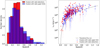 |
Fig. 3 Left: histogram showing the redshift distribution of the sample, classified into radio detections (red) and upper limits (blue). Right: LX500 vs. redshift for the sample. The dashed line denotes the theoretical flux cut of the eROSITA observation. |
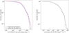 |
Fig. 4 Left: X-ray luminosity distribution for the parent sample of clusters and groups divided into objects with (red) and without (blue) radio detection. Right: radio luminosity distribution for clusters and groups with radio detection. |
3 Analysis and discussion
3.1 X-ray and radio luminosity distributions
In Fig. 4, we show the X-ray and radio luminosity distributions. The X-ray distribution, in the left panel, spans the range from LX,500 kpc ~ 1041 ergs−1 to 4×1044 ergs−1 for objects with radio detections, while the range for clusters with upper limits is slightly narrower, reaching 3 × 1044 erg s−1. Due to the high sensitivity of eROSITA, we are able to reach lower luminosities than the existing X-ray samples of clusters and groups. The BCS sample, compiled with rOsAT (Ebeling et al. 1997), reaches LX ~ 1042 erg s−1, similarly to the REFLEX II catalogue (Böhringer et al. 2014). On the other hand, our upper range is lower than both the BCS and the REFLEX II, which extend well beyond LX ~ 1045 erg s−1, because our sample comes from a relatively small field in the sky. The forthcoming eROSITA all-sky survey (eRASS, Bulbul et al., in prep.) will observe a large number of clusters and groups, allowing us to extend our analysis to higher luminosities.
The radio luminosity distribution at 144 MHz, in the right panel, ranges from L144MHz ~ 1029 erg s−1 Hz−1 to ~1034 ergs−1 Hz−1. Given the assumption on the spectral index made above, the upper range of luminosities at 144 MHz corresponds to L1.4GHz ~ 1.6× 1033 ergs−1 Hz−1. This is lower than other samples that have recently been studied at this frequency. The catalogue of 1.4 GHz radio sources in galaxy groups analysed in P20 reaches L1.4GHz ~ 1034 ergs−1 Hz−1, similarly to the sample of BCG radio galaxies by Hogan et al. (2015). Finally, we note that the sample studied at 235 MHz by Kolokythas et al. (2018, 2019) ranges from L235 MHz ~ 1027 to 1032 ergs−1 Hz−1. Converting from 144MHz luminosity, eFEDS radio galaxies span from L235 MHz ~ 6.8 × 1028 to 6.7 × 1033 erg s−1 Hz−1. Therefore our sample extends to higher radio powers, but does not reach as deeply as CLoGS. Nevertheless, it consists of 227 clusters and groups, compared to the 53 groups that belong to CLoGS.
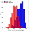 |
Fig. 5 BCG offsets from the X-ray emission peak, assumed as the centre of the cluster or group, for galaxies with AGN radio emission (red) and for those with radio upper limits (blue). |
3.2 BCG offsets
Figure 5 shows the histogram of the BCG offset from the centre of the host cluster or group. The centre was estimated by fitting a two-dimensional β-model (Cavaliere & Fusco-Femiano 1976) to the X-ray emission. Most BCGs with detected AGN radio emission lie within ~50 kpc from the cluster centre (~84%). For these clusters, the median value of the offset distribution is ~ 15 kpc, with dispersion ~ 30 kpc. At larger offsets, it is easier to find BCGs that do not host a radio galaxy. For clusters with no radio detection, the median is ~ 130 kpc with a dispersion of ~ 190 kpc.
Small offsets (<50 kpc) are expected and found in most relaxed clusters because even a minor merger can induce sloshing and displace the X-ray emission peak from the BCG (e.g. Hamer et al. 2016; Pasini et al. 2019, 2021b; Ubertosi et al. 2021). Large offsets (100-1000 kpc) are often an indication of a strongly disturbed cluster environment (Rossetti et al. 2016; De Propris et al. 2021, and references therein). The relation of BCGs, the triggering of the AGN, and the offset from the cluster centre has been widely discussed and was recently studied in Pasini et al. (2021a). In that paper, the authors found that it is more common for more central BCGs to show radio-loud AGN because in these galaxies the accretion onto the central BH is boosted by the strong cooling in the cluster core. Similar results have also been discussed in Burns (1990), Best et al. (2007), Cavagnolo et al. (2008) and Shen et al. (2017). On the other hand, off-centre galaxies have to rely on more episodic processes, such as cluster and group mergers and/or galaxy interactions. We find the same results in this sample because, as discussed above, radio-loud AGNs are mostly found at an offset <50 kpc.
3.3 Extent of BCG radio galaxies
Radio galaxies exhibit a plethora of different shapes and sizes. The reasons for the unusual size of some giant radio galaxies (e.g. Brüggen et al. 2021; Dabhade et al. 2020) and for the significantly smaller extent of some others (e.g. FR0, Baldi et al. 2015) have been investigated previously. Hardcastle et al. (2019) presented the currently largest sample of radio galaxies in which the relation between the radio power and the linear size was investigated. The location of a source in this diagram is indicative of its initial conditions and current evolutionary state (Hardcastle 2018). Kolokythas et al. (2018) found a clear link between the 235 MHz power and the projected largest linear size (LLS) of their resolved radio galaxies. The same relation was already found for cluster and field radio galaxies by Ledlow et al. (2002) and is investigated for our sample of BCGs at 144 MHz (top panel of Fig. 6). The LLS of radio galaxies was manually measured from the LOFAR eFEDS mosaic, assuming an error equal to the synthesised beam. To exclude unresolved sources, only those with a largest angular size LAS >2 × beam were taken into account.
Most sources show an LLS between 100 and 300 kpc, with the mean at LLS~235 kpc and standard deviation ~ 160 kpc. Large sources mostly show a classical double-lobed morphology, while the smallest ones are point-like. As previously observed, there is a positive correlation between LLS and luminosity, with larger radio galaxies being more powerful. The relation holds even at relatively high luminosities5. Nevertheless, we note that we are likely missing large, low-power radio sources because of surface brightness limitations. This issue has been extensively addressed in Hardcastle et al. (2019) based on a significantly larger sample (23 344 objects) of radio galaxies.
Multiple environmental factors are likely to contribute to the size of the radio source. The most important factor is the age, which necessarily introduces scatter into any relation with other physical quantities. Other factors include the location of the galaxy within the host cluster, the density of the ICM at the position of the galaxy, the efficiency of the accretion onto the AGN, and the radio power of the outburst (see e.g. Moravec et al. 2020, and references therein).
To this end, in the bottom panel of Fig. 6 we show the LLS of the radio galaxy plotted against the central density (at R = 0.02R500) of the host cluster, obtained by fitting the cluster model by Vikhlinin et al. (2006) to density profiles (see G22 for further details). We see no correlation of the LLS with the central density, suggesting that radio power is more prominent than ambient density in determining the size of the radio galaxy and that the contribution of other factors could affect a possible link.
3.4 Correlation between X-ray and 144 MHz radio luminosity
In P20, we have studied the correlation between the 1.4 GHz power of radio galaxies and the X-ray luminosity of the host group for 247 galaxy groups in COSMOS. A similar correlation between the mass of galaxy clusters, known to correlate with the X-ray luminosity (e.g. Lovisari et al. 2020), and the radio power of BCGs has been found by Hogan et al. (2015). Here, we focus on the same relation, but at the lower radio frequency of 144 MHz.
Figure 7 shows the 144 MHz power of the radio galaxy plotted against the X-ray luminosity of the host group or cluster. The size of the symbols is proportional to the LLS of the radio sources, and the colour corresponds to the redshift. Upper limits are represented by downward-pointing arrows. There is a clear trend for stronger radio galaxies to be hosted in more X-ray luminous clusters, as found by P20. However, the significant number of radio upper limits makes it harder to determine whether the observed correlation is real or produced by selection effects set by the sensitivity of the observation.
To ascertain if the correlation is genuinely detected, we performed the partial correlation Kendall’s τ (Akritas & Siebert 1996) test. This tool has already been used in a number of papers (e.g. Ineson et al. 2015; Pasini et al. 2020) to test correlations in the presence of upper limits and redshift dependence. The algorithm estimates the null-hypothesis probability that selection effects produce the correlation. If the probability is low, then it is likely that the correlation is real. The test performed on our sample gives a null-hypothesis probability p < 0.0001% (τ = 0.1178, σ = 0.0227), indicating that the correlation is real and not generated by selection effects. This result is consistent with P20, who also found that such a correlation, but at higher frequency, was not produced by biases.
Bianchi et al. (2009) argued that the Kendall τ test may underestimate the redshift contribution, particularly when the significance and the functional relation are to be determined. For this reason, they performed a ‘scrambling’ test that has also been used in other works (e.g. Merloni et al. 2006). The principle of this algorithm is to keep each Lx/z pair because their association comes from the source selection. Then they shuffled the corresponding radio fluxes, assigning them to a new Lx/z pair. The new radio luminosity is then computed at the new redshift (see Eq. (2)). If the correlation is real, it is expected to disappear when the luminosity pairs are shuffled. We applied this test 100 times and estimated for each cycle the null-hypothesis probability through the Kendall τ test. The results are shown in Fig. 8. In 100 cycles, the null-hypothesis probability is never found to be lower than the real sample. The mean probability value lies at ~4%, with a standard deviation of ~9%, while the peak lies between 0.7% and 5%. This result supports the hypothesis that the observed correlation is real.
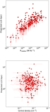 |
Fig. 6 Top: projected LLS vs. radio power of eFEDS radio galaxies. Bottom: projected LLS of the radio galaxy vs. ICM central density. |
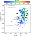 |
Fig. 7 144 MHz power of radio galaxies vs. X-ray luminosity of the host cluster. Symbol sizes are proportional to the LLS of the source, and their colour indicates the redshift. Downward-pointing arrows denote radio upper limits. Bars represent errors on both axes. |
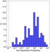 |
Fig. 8 Null-hypothesis probability distribution that the correlation is not real for 100 mock datasets produced by the scrambling test. The dashed red line indicates the probability of the real sample. |
3.5 X-ray/radio correlation at 1.4 GHz
We compared our 144 MHz sample in eFEDS with a subsample of 137 systems from the 247 COSMOS galaxy groups studied at 1.4 GHz in P20. A further cross-match of our sample with all-sky surveys at this frequency (e.g. NVSS, Condon et al. 1998) is not trivial because of the significant differences in surface brightness sensitivity and resolution. For this reason, the 144 MHz luminosities were converted into luminosities at a frequency of 1.4 GHz assuming α = 0.8 ± 0.2. The assumed uncertainty on the spectral index dominates the previous 144 MHz flux error. Combining the two catalogues, we obtain 364 galaxy clusters and groups that allow us to assess the radio/X-ray correlation using a larger sample. The corresponding log LR–log LX plot is shown in Fig. 9.
The distributions of COSMOS and eFEDS clusters and groups agree well. This is confirmed by the two-dimensional Kolmogorov-Smirnov test, which gives p = 0.41 under the null-hypothesis that the two samples are drawn from the same parent distribution. This implies that our assumption of a uniform spectral index of α = 0.8 for every radio galaxy is valid, although it introduces more scatter in the correlation. Still, a clear trend for more massive groups and clusters hosting more powerful radio sources is seen. This is also supported by the Kendall τ test, which results in p < 0.0001 (τ = 0.1331, σ = 0.0138) for eFEDS+COSMOS. The best-fit relation was estimated by exploiting the parametric EM algorithm coded in the AStronomical SURVival statistics package (ASURV, Feigelson et al. 2014), which takes into account different contributions by detections and upper limits. We find log Lr = (0.84 ± 0.09) log Lx−(6.46 ± 4.07). This estimate is marginally consistent with the best-fit relations of P20 (log Lr = (1.07 ± 0.12) × log Lx−(15.90 ± 5.13) and Pasini et al. (2021a) (log Lr = (0.94 ± 0.43) × log Lx−(9.53 ± 18.19)), obtained through the same method and applying Bayesian inference, respectively.
The correlation may imply a link between radiative cooling from the ICM and the more variable and episodic activity of the AGN. Because the X-ray luminosity is predominantly driven by the cluster or group mass, this correlation may be produced by massive clusters hosting more massive BCGs and in turn more massive BHs. In relaxed clusters, the cooling of the ICM is able to efficiently feed the central AGN, leading to higher radio powers (Soker & Pizzolato 2005; Gaspari et al. 2011). This is reflected in the well-studied link between the cavity power of systems hosting X-ray bubbles and the luminosity of the cluster cooling region (e.g. Bîrzan et al. 2004, 2017; Rafferty et al. 2006). Sun (2009) also argued that small coronae of X-ray emitting gas in BCGs are able to trigger strong radio outbursts long before cool cores are formed in the host cluster, leading to heating in their surroundings and even preventing their formation, especially in low-mass systems. The correlation presented here shows a large scatter, especially at high luminosities. This might for instance be caused by differences in the dynamical states, which we explore in the next section.
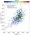 |
Fig. 9 1.4 GHz power of radio galaxies vs. X-ray luminosity of the host cluster for the eFEDS and P20 samples. The colours correspond to the redshift. eFEDS data are represented by circles, while diamonds are COSMOS systems. Downward-pointing arrows denote radio upper limits. Bars represent errors on both axes. Errors on the y-axis are dominated by the assumed uncertainty on the spectral index. The best-fit relation is shown in grey: log LR = (0.84 ± 0.09) log LX−(6.46 ± 4.07). |
3.6 Kinetic luminosity and AGN feedback
The radio luminosity is a measure of the instantaneous radiative loss rate of the radio lobes, and as such is only indirectly related to the energy produced by the AGN through accretion onto the SMBH. For an active source, only a small fraction of the total power supplied to the lobes has been radiated away at any given time, while a much larger fraction is stored in the lobes and a similar amount has been dissipated into the surrounding ICM during the expansion of the jets through the ICM (Willott et al. 1999; Smolcic et al. 2017). The latter, which we refer to as kinetic luminosity, is directly linked to the heating of the ICM and contributes to quenching the radiative losses of the hot plasma (see Sect. 1 for references).
The relation of the kinetic and radio luminosity has been the subject of many works (e.g. Willott et al. 1999; Bîrzan et al. 2004, 2008; Cavagnolo et al. 2010; O’Sullivan et al. 2011b; Smolcic et al. 2017). As thoroughly discussed in Hardcastle et al. (2019), there are currently two methods to infer the kinetic luminosity. The first relies on the identification of X-ray cavities and is affected by assumptions on the cavity age and biased towards small sources in cluster-rich environments (Bîrzan et al. 2012). The second method relies on a conversion based on a theoretical model and, as such, can lead to unrealistic results if the contribution of source age, environment, and redshift to the radio luminosity are not taken into account properly. We refer to Hardcastle et al. (2019) and Appendix A of Smolčić et al. (2017) for a detailed discussion of this scaling relation. Here, we assume the relation adopted by Willott et al. (1999) to convert into the 1.4 GHz rest-frame luminosity (Heckman & Best 2014),
 (3)
(3)
where Lkin,1.4GHz is the kinetic luminosity, L1.4GHz is the luminosity as measured at 1.4 GHz, and fW is an uncertainty parameter that we assumed, fW = 15, as estimated by X-ray observations of ICM bubbles in galaxy clusters (e.g. Merloni & Heinz 2007; Bîrzan et al. 2008). We determined the kinetic luminosity for the radio galaxies of the eFEDS and the P20 sample, and we compared it to the X-ray luminosity within 500 kpc of the host cluster. The result is shown in Fig. 10.
In order to infer the relation of the X-ray and the kinetic luminosity, we applied Bayesian inference on the two samples using the linmix6 package (Kelly 2007). With this tool, we performed a linear fit in the log-log scale of the form
 (4)
(4)
with α and β representing the intercept and the slope, respectively, while e is the intrinsic scatter of the relation. We find α = −2.19 ± 4.05, β = 1.07 ± 0.11 and ϵ = 0.25 ± 0.05. We note that the conversion from radio into kinetic luminosity, which also depends on external factors such as the morphology and age of the radio source, the extrapolation of 1.4 GHz fluxes, or the surrounding environment, and which relies on theoretical models, may have introduced artificial scatter into the correlation.
Nevertheless, the plot suggests that in most clusters and groups, the heating from the central AGN efficiently counterbalances the ICM radiative losses, as has been found in a large number of publications (see the references above and McNamara & Nulsen 2007, 2012 for reviews). However, most of these papers take the luminosity from within the cooling region into account, which is usually defined as the cluster region within which the cooling time of the ICM is shorter than 7.7 Gyr. These usually range between ~50 and ~ 150 kpc (Bîrzan et al. 2017), and their extent can only be estimated through a deprojected analysis of the thermodynamical profiles (i.e. temperature, density, and cooling time) derived from X-ray observations. The detection of cavities as an indication for AGN heating (McNamara et al. 2000; Bîrzan et al. 2004) usually requires deep, high-resolution X-ray observations as well.
The kinetic luminosity–X-ray luminosity relation, estimated through survey data but with the unprecedented sensitivity of eROSITA is able to provide a first insight into the processes of AGN feedback of a large number of clusters and groups. Kinetic and X-ray luminosity act as proxy for mechanical feedback and cooling luminosity, respectively, which together constitute the ‘parent’ correlation usually found in cool core clusters. Nevertheless, we performed the analysis on all our objects and did not distinguish between cool cores and merging clusters. Main et al. (2017) found that in their sample of clusters, this correlation only holds for cool cores. Their classification was based on the central cooling time, determined through Chandra observations at 0.004R500 by Hudson et al. (2010). The eROSITA observations do not yield cooling times at such small cluster-centric radii, and we are not able to reproduce the same classification for our objects. Instead, we quantified the dynamical state of clusters through the concentration parameter as defined in Lovisari et al. (2017) and estimated for eFEDS clusters in G22 as
 (5)
(5)
where sB is the surface brightness estimated inside 0.1R500 for the numerator and inside R500 for the denominator. This parameter is an indicator of a centrally peaked X-ray surface brightness profile, which correlates with the dynamical state of the cluster. Lovisari et al. (2017) discussed the use of different thresholds to classify clusters into cool cores and disturbed systems, showing how completeness (i.e. being able to select all clusters belonging to a given class) and purity (i.e. being able to securely assign clusters to a given class) change depending on the chosen threshold. Here, following the work cited above, we chose to define as non-cool cores (NCC) clusters with cSB < 0.15, while cool cores (CC) have cSB > 0.27. This classification allows for 100% purity for both subsamples, but the completeness decreases to ~53% for CC and ~75% for NCC (see Lovisari et al. 2017 for more details). Clusters with 0.15 < cSB < 0.27 cannot be securely categorised and are arbitrarily referred to as moderately cool cores (MCC). In the left panel of Fig. 11 we show the Lkin−LX plot for the eFEDS cluster sample, in which clusters were classified through the concentration parameter. We find that ~53% of clusters are NCC, ~28% are MCC, and ~19% are CC. We see no obvious difference in the distribution between the three subsamples. Therefore the dynamical state of the cluster does not seem to have a large effect on the scatter in the X-ray/radio relation.
As discussed in more detail in G22, the concentration acts as an indicator of a cool core. However, while a relaxed cluster will generally present a cool core, a cool core is not always an indication of relaxation: a merger in its initial stage predominantly affects the cluster outskirts and does not disrupt the cool core (see e.g. theoretical work by Rasia et al. 2015 and Biffi et al. 2016). This means that classifying the dynamical state of clusters based on concentration alone is useful to distinguish disturbed objects with low concentration, but does not provide a clear identification of relaxed clusters (see Fig. 9 of G22 and related discussion). For this reason, we performed an alternative classification based on a new morphological parameter first introduced in the same paper, the so-called relaxation score (Rscore). Because a complete, physical definition of this parameter requires detailed discussion of a number of parameters (see below), we refer to G22 for more insights, and provide a brief description here. The Rscore combines a number of morphological parameters that are usually determined for galaxy clusters, such as concentration, central density, ellipticity (ratio of the minor and major axes of the cluster), and cuspiness (slope of the density profile at a given radius). The resulting Rscore provides a clearer indication than concentration alone of the dynamical state of a cluster. In particular, the Rscore should be higher for relaxed objects, which show a high concentration, central density, ellipticity, and cuspiness. On the other hand, the same parameter should decrease in disturbed clusters.
Following the discussion in G22, we defined as relaxed objects with Rscore > 0.0137. The results of this alternative classification are shown in the right panel of Fig. 11. We only plot clusters for which a proper estimate of the Rscore was feasible in G22. Objects classified as relaxed through the Rscore and as CC through the concentration are generally referred to as CC, those with low Rscore and concentration are NCC, and clusters with a high concentration (same threshold as used for left panel) but Rscore < 0.0137 are labelled unclear. We refer to G22 for a discussion and comparisons of the different classifications and focus on the correlation here.
Even when a more accurate parameter such as the Rscore is introduced, the distinction in the distribution between cool cores and merging objects is still unclear, as was instead found in Main et al. (2017), for instance. Furthermore, it is not clear how this relation can be present in disturbed systems. In these objects, the cooling of the ICM is slow and BCGs are often hard to identify. Morphological parameters have been widely used to determine the dynamical state of clusters, but a more secure classification based on the central cooling time may be more useful for understanding in which clusters a connection of AGN and cooling ICM can ensue. A possibility is that the link between AGN and their environment could be produced, even in disturbed objects, by rapidly cooling coronae permeating the host galaxy (Sun et al. 2007; Gastaldello et al. 2008; Sun 2009). This idea has been suggested for NCC hosting radio AGN, such as A2028 (Gastaldello et al. 2010). It is also plausible that small, low-entropy regions of the cluster core such as cool core remnants (Rossetti & Molendi 2010) could affect the AGN, leading to the observed relation. Another possibility is that NCC do not in fact belong to the correlation. To test this, we studied the scatter of the correlation after applying Bayesian inference only on CC. If NCC are not part of the correlation, the scatter of the data should decrease when CC are fitted alone. We find ϵ = 0.17 ± 0.10, consistent within errors with the previous estimate. Nevertheless, the uncertainty increases because of the relatively small number of CC, and further analyses exploiting larger samples are needed to investigate this further.
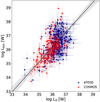 |
Fig. 10 Kinetic luminosity of BCG radio galaxies estimated at 1.4 GHz vs. X-ray luminosity of the host cluster or group for the eFEDS (blue) and P20 (red) samples. The black line represents the best-fit estimated from Bayesian inference: log Lkin = (1.07 ± 0.11)log LX−(2.19 ± 4.05). The grey area indicates 1σ errors. |
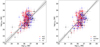 |
Fig. 11 Left: kinetic luminosity of BCG radio galaxies estimated at 1.4 GHz vs. X-ray luminosity of the host cluster or group for the eFEDS sample. Data are classified into non-cool cores (red), moderately cool cores (blue), and cool cores (black) based on the concentration parameter. Right: same as in the left panel, with data classified based on the Rscore (see discussion). |
4 Conclusions
We used eROSITA (X-ray) and LOFAR (radio) observations of the eFEDS field in order to investigate radio galaxies hosted in BCGs. Our results are summarised below:
Our sample yields 227 detections and 248 upper limits in the redshift range 0.01 < z < 1.3 and luminosity range 1022−1027 WHz−1 at 144 MHz. The remaining 67 clusters were excluded from the analysis to avoid contamination by misclassified AGN (see Sect. 2.3). The radio detection rate is ~48%, which is lower than in other samples of well-studied groups and clusters;
BCGs hosting radio-loud AGN mostly (~84%) lie within 50 kpc from the cluster centre. BCGs that are more offset tend to have lower levels of radio emission or lie below our detection threshold;
As was argued in previous works, larger radio galaxies are usually more powerful. However, we note that a relevant selection effect is present in our sample because we lack large, low-power radio sources because of limited sensitivity. We see no correlation of the central cluster density (R = 0.02R500) with the LLS, suggesting that the luminosity is a better predictor for the size of the radio galaxy;
We studied the relation of the 144 MHz radio galaxy power and the host cluster X-ray luminosity measured within 500 kpc from the cluster centre and found a positive correlation. Because of the large number of upper limits, we relied on statistical tests, such as the partial correlation Kendall’s τ test and the scrambling test, to show that the correlation is not produced by selection effects in the radio band;
Converting the 144 MHz power of radio galaxies into 1.4 GHz, we compared our results with the correlation between the X-ray luminosity and the 1.4 GHz power of a COSMOS galaxy groups sample first investigated by Pasini et al. (2020). We found that the two samples agree well based on a Kolmogorov-Smirnov test, which under the nullhypothesis that the samples are drawn from the same parent distribution, gives p = 0.41. We estimated a best-fit relation log Lr = (0.84 ± 0.09) log Lx−(6.46 ± 4.07);
We converted the radio powers of radio galaxies into kinetic luminosities, making use of widely used scaling relations. Comparing the kinetic luminosity to the X-ray luminosity within 500 kpc from the cluster centre, we found that in most objects the ICM radiative losses are efficiently counterbalanced by heating supplied from the central AGN. We derived the best-fit relation applying Bayesian inference, obtaining log Lkin = (−2.19 ± 4.05) + (1.07 ± 0.11) log Lx + (0.25 ± 0.05);
We classified eFEDS clusters into disturbed and relaxed objects based on two different parameters: concentration, and the relaxation score (see Sect. 3.6 for a definition). No significant differences in the Lkin−Lx relation of the subsamples were visible.
Future prescriptions of radio-mode AGN feedback in simulations need to be able to recover the properties described in this paper. In addition to massive halo gas fractions, entropy slopes, and galaxy properties, they need to recover radio luminosities as a function of the host cluster properties. With the new all-sky X- ray surveys, a correlation between the cluster X-ray luminosity and the BCG radio power can be used to probe AGN feedback across a wider range of host masses and to control for the effect of other observables. Particularly, the synergy between eRASS (Bulbul et al., in prep.) and the lOfAR Two-Metre Sky Survey (LoTSS, Shimwell et al. 2017), as well as the forthcoming LOFAR LBA Sky Survey (LoLSS, de Gasperin et al. 2021), will provide samples of thousands of clusters and groups for which the interplay between the AGN and the ICM can be investigated.
Acknowledgements
The authors thank the anonymous referee for useful suggestions that have improved the presentation of the results. T.P. thanks Philip Best for useful comments. T.P. is supported by the BMBF Verbundforschung under grant number 50OR1906. M.B. acknowledges support from the Deutsche Forschungs- gemeinschaft under Germany’s Excellence Strategy–EXC 2121 “Quantum Universe”–390833306. D.N.H. acknowledges support from the ERC through the grant ERC-Stg DRANOEL no. 714245. A.B. acknowledges support from the VIDI research programme with project number 639.042.729, which is financed by the Netherlands Organisation for Scientific Research (NWO). F.G. acknowledges support from INAF mainstream project ‘Galaxy Clusters Science with LOFAR’ 1.05.01.86.05. R.J.vW. acknowledges support from the ERC Starting Grant ClusterWeb 804208. W.L.W. acknowledges support from the CAS-NWO programme for radio astronomy with project number 629.001.024, which is financed by the Netherlands Organisation for Scientific Research (NWO). This work is based on data from eROSITA, the soft X-rays instrument aboard SRG, a joint Russian-German science mission supported by the Russian Space Agency (Roskosmos), in the interests of the Russian Academy of Sciences represented by its Space Research Institute (IKI), and the Deutsches Zentrum für Luft- und Raumfahrt (DLR). The SRG spacecraft was built by Lavochkin Association (NPOL) and its subcontractors, and is operated by NPOL with support from the Max Planck Institute for Extraterrestrial Physics (MPE). The development and construction of the eROSITA X-ray instrument was led by MPE, with contributions from the Dr. Karl Remeis Observatory Bamberg & ECAP (FAU Erlangen-Nuernberg), the University of Hamburg Observatory, the Leibniz Institute for Astrophysics Potsdam (AIP), and the Institute for Astronomy and Astrophysics of the University of Tübingen, with the support of DLR and the Max Planck Society. The Argelander Institute for Astronomy of the University of Bonn and the Ludwig Maximilians Universität Munich also participated in the science preparation for eROSITA. The eROSITA data shown here were processed using the eSASS/NRTA software system developed by the German eROSITA consortium. LOFAR data products were provided by the LOFAR Surveys Key Science project (LSKSP; https://lofar-surveys.org/) and were derived from observations with the International LOFAR Telescope (ILT). LOFAR (van Haarlem et al. 2013) is the Low Frequency Array designed and constructed by ASTRON. It has observing, data processing, and data storage facilities in several countries, that are owned by various parties (each with their own funding sources), and that are collectively operated by the ILT foundation under a joint scientific policy. The efforts of the LSKSP have benefited from funding from the European Research Council, NOVA, NWO, CNRS-INSU, the SURF Co-operative, the UK Science and Technology Funding Council and the Jülich supercomputing centre.
Appendix A Examples of interesting systems
The high flux sensitivity and spatial coverage of eROSITA and LOFAR at their respective frequencies allows for interesting comparisons. In the past, the combination of X-ray and radio observations of galaxy clusters and of their BCGs have led to a significant improvement in the understanding of the thermal and non-thermal processes in these environments (e.g. Gitti et al. 2010; Kolokythas et al. 2018; Botteon et al. 2020; see Sect. 1 for more references and reviews).
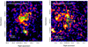 |
Fig. A.1 eROSITA 0.2-2.3 keV images of eFEDSJ085022.3+001607 (left panel) and eFEDSJ085830.1-010656 (right panel), smoothed with a 3σ Gaussian filter. LOFAR 144 MHz contours at 3, 6, 12, 24 × rms (local) are plotted in green. The white cross represents the cluster X-ray peak, and the yellow cross is the BCG position. For eFEDSJ085830.1-010656, the BCG is coincident with the X-ray peak. |
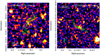 |
Fig. A.2 eROSITA 0.2-02.3 keV images of eFEDSJ091322.9+040618 (left panel) and eFEDSJ093056.f9+034826 (right panel), smoothed with a 3σ Gaussian filter. LOFAR 144 MHz contours at 3, 6, 12, 24 × rms (local) are plotted in green. The white cross represents the cluster X-ray peak. For eFEDSJ091322.9+040618, the BCG is coincident with the X-ray peak. |
We used the eROSITA and LOFAR observations to search for systems showing interesting morphologies and signs of possible interaction between the ICM and the central AGN. In this section, we present four of the most interesting examples of these clusters. We focus on AGN emission, and diffuse emission more directly associated with the ICM and clusters dynamical state will be presented in a forthcoming paper (Hoang et al., in prep.). Table A.1 summarises the main properties of these systems.
A.0.1 eFEDSJ085022.3+001607
eFEDSJ085022.3+001607 (left panel of Fig. A.1) is located at a redshift of z = 0.196 (spectroscopic). The strongly elliptical and irregular morphology of the X-ray emission and low concentration (cSB = 0.02) suggest that this cluster is disturbed. The BCG hosts an elongated, head-tail shaped radio galaxy (major axis ~500 kpc), with a 144 MHz luminosity of LR = (4.1 ± 0.2) × 1024 WHz−1. The AGN lies at ~150 kpc from the X-ray peak. Surface brightness discontinuities that coincide with the lobes of the radio galaxy are detected in the X-ray image. However, the relatively low resolution does not reveal any ICM cavities, which have never been detected around head-tails, however. The shape of the non-thermal emission follows that of the hot plasma, with the jet extending towards the east through the X-ray ripple. Meanwhile, the expansion in the opposite direction appears to be halted.
X-ray observables and BCG radio power for four relevant eFEDS clusters.
A.0.2 eFEDSJ085830.1-010656
The irregular morphology and low concentration (cSB = 0.13) of eFEDSJ085830.1-010656 (right panel of Fig. A.1) leads us to classify it as a non-cool core. The BCG hosts a wide-angle tail radio galaxy with two tails departing in the S and SW directions for ~250 kpc each. The tails are expanding into a lower-density region within the group. Deeper X-ray observations are needed to study the ICM emission of this group because of its low surface brightness and relatively high redshift.
A.0.3 eFEDSJ091322.9+040618
eFEDSJ091322.9+040618 (left panel of Fig. A.2) is a low- redshift (z = 0.088, spectroscopic) galaxy group classified as a disturbed cluster due to its irregular shape and low concentration (cSB = 0.04). The radio galaxy extends for more than 200 kpc along the NW-SE axis. The lobes are expanding into the SE and NW directions following the hot plasma. Diffuse emission with unclear origin is detected in the SE direction, correspondingly to a low surface brightness region, extending for ~ 150 kpc.
A.0.4 eFEDSJ093056.9+034826
eFEDSJ093056.9+034826 (right panel of Fig. A.2) is a galaxy group located at z = 0.09 (photometric). The elliptical shape and relatively high concentration (cSB = 0.21) classify it as a moderately cool core. The BCG hosts a double-lobe elongated radio galaxy with a major axis of ~600 kpc and LR = (7.7 ± 0.2) × 1023 W Hz−1. The long lobes (~300 kpc) of the central radio galaxy extend far beyond the X-ray bright core of the group. The low X-ray flux of this group makes it difficult to identify depressions in the surface brightness.
References
- Aihara, H., Arimoto, N., Armstrong, R., et al. 2018, PASJ, 70, S4 [NASA ADS] [Google Scholar]
- Akritas, M. G., & Siebert, J. 1996, MNRAS, 278, 919 [NASA ADS] [CrossRef] [Google Scholar]
- Alexander, D. M., Swinbank, A. M., Smail, I., McDermid, R., & Nesvadba, N. P. H. 2010, MNRAS, 402, 2211 [CrossRef] [Google Scholar]
- Baldi, R. D., Capetti, A., & Giovannini, G. 2015, A&A, 576, A38 [NASA ADS] [CrossRef] [EDP Sciences] [Google Scholar]
- Best, P. N., Kauffmann, G., Heckman, T. M., et al. 2005, MNRAS, 362, 25 [Google Scholar]
- Best, P. N., von der Linden, A., Kauffmann, G., Heckman, T. M., & Kaiser, C. R. 2007, MNRAS, 379, 894 [Google Scholar]
- Bharadwaj, V., Reiprich, T.H., Schellenberger, G., et al. 2014, A&A, 572, A46 [NASA ADS] [CrossRef] [EDP Sciences] [Google Scholar]
- Bharadwaj, V., Reiprich, T. H., Lovisari, L., & Eckmiller, H. J. 2015, A&A, 573, A75 [NASA ADS] [CrossRef] [EDP Sciences] [Google Scholar]
- Bianchi, S., Bonilla, N. F., Guainazzi, M., Matt, G., & Ponti, G. 2009, A&A, 501, 915 [NASA ADS] [CrossRef] [EDP Sciences] [Google Scholar]
- Biffi, V., Borgani, S., Murante, G., et al. 2016, ApJ, 827, 112 [NASA ADS] [CrossRef] [Google Scholar]
- Bîrzan, L., Rafferty, D. A., McNamara, B. R., Wise, M. W., & Nulsen, P. E. J. 2004, ApJ, 607, 800 [Google Scholar]
- Bîrzan, L., McNamara, B. R., Nulsen, P. E. J., Carilli, C. L., & Wise, M. W. 2008, ApJ, 686, 859 [Google Scholar]
- Bîrzan, L., Rafferty, D. A., Nulsen, P. E. J., et al. 2012, MNRAS, 427, 3468 [Google Scholar]
- Bîrzan, L., Rafferty, D. A., Brüggen, M., & Intema, H. T. 2017, MNRAS, 471, 1766 [CrossRef] [Google Scholar]
- Blanton, M. R., Bershady, M. A., Abolfathi, B., et al. 2017, AJ, 154, 28 [Google Scholar]
- Böhringer, H., Chon, G., & Collins, C. A. 2014, A&A, 570, A31 [NASA ADS] [CrossRef] [EDP Sciences] [Google Scholar]
- Botteon, A., Brunetti, G., van Weeren, R. J., et al. 2020, ApJ, 897, 93 [Google Scholar]
- Brüggen, M., Reiprich, T. H., Bulbul, E., et al. 2021, A&A, 647, A3 [NASA ADS] [CrossRef] [EDP Sciences] [Google Scholar]
- Brunner, H., Liu, T., Lamer, G., et al. 2022, A&A, 661, A1 (eROSITA EDR SI) [NASA ADS] [CrossRef] [EDP Sciences] [Google Scholar]
- Burns, J. O. 1990, AJ, 99, 14 [NASA ADS] [CrossRef] [Google Scholar]
- Cavagnolo, K. W., Donahue, M., Voit, G. M., & Sun, M. 2008, ApJ, 683, L107 [Google Scholar]
- Cavagnolo, K. W., Donahue, M., Voit, G. M., & Sun, M. 2009, ApJS, 182, 12 [Google Scholar]
- Cavagnolo, K. W., McNamara, B. R., Nulsen, P. E. J., et al. 2010, ApJ, 720, 1066 [Google Scholar]
- Cavaliere, A., & Fusco-Femiano, R. 1976, A&A, 49, 137 [NASA ADS] [Google Scholar]
- Condon, J. J., Cotton, W. D., Greisen, E. W., et al. 1998, AJ, 115, 1693 [Google Scholar]
- Croton, D. J., Springel, V., White, S. D. M., et al. 2006, MNRAS, 365, 11 [Google Scholar]
- Dabhade, P., Röttgering, H. J. A., Bagchi, J., et al. 2020, A&A, 635, A5 [NASA ADS] [CrossRef] [EDP Sciences] [Google Scholar]
- de Gasperin, F., Dijkema, T. J., Drabent, A., et al. 2019, A&A, 622, A5 [NASA ADS] [CrossRef] [EDP Sciences] [Google Scholar]
- de Gasperin, F., Williams, W. L., Best, P., et al. 2021, A&A, 648, A104 [NASA ADS] [CrossRef] [EDP Sciences] [Google Scholar]
- De Propris, R., West, M. J., Andrade-Santos, F., et al. 2021, MNRAS, 500, 310 [Google Scholar]
- Dey, A., Schlegel, D. J., Lang, D., et al. 2019, AJ, 157, 168 [Google Scholar]
- Driver, S. P., Norberg, P., Baldry, I. K., et al. 2009, Astron. Geophys., 50, 5.12 [NASA ADS] [CrossRef] [Google Scholar]
- Dunn, R. J. H., Allen, S. W., Taylor, G. B., et al. 2010, MNRAS, 404, 180 [NASA ADS] [Google Scholar]
- Ebeling, H., Edge, A. C., Fabian, A. C., et al. 1997, ApJ, 479, L101 [NASA ADS] [CrossRef] [Google Scholar]
- Ehlert, S., Allen, S. W., von der Linden, A., et al. 2011, MNRAS, 411, 1641 [NASA ADS] [CrossRef] [Google Scholar]
- Fabian, A. C., Sanders, J. S., Taylor, G. B., et al. 2006, MNRAS, 366, 417 [NASA ADS] [CrossRef] [Google Scholar]
- Feigelson, E. D., Nelson, P. I., Isobe, T., & LaValley, M. 2014, ASURV: Astronomical SURVival Statistics, Astrophysics Source Code Library [record ascl:1406.001] [Google Scholar]
- Gaspari, M., Melioli, C., Brighenti, F., & D’Ercole, A. 2011, MNRAS, 411, 349 [Google Scholar]
- Gaspari, M., Tombesi, F., & Cappi, M. 2020, Nat. Astron., 4, 10 [Google Scholar]
- Gastaldello, F., Buote, D. A., Brighenti, F., & Mathews, W. G. 2008, ApJ, 673, L17 [NASA ADS] [CrossRef] [Google Scholar]
- Gastaldello, F., Buote, D. A., Temi, P., et al. 2009, ApJ, 693, 43 [NASA ADS] [CrossRef] [Google Scholar]
- Gastaldello, F., Ettori, S., Balestra, I., et al. 2010, A&A, 522, A34 [NASA ADS] [CrossRef] [EDP Sciences] [Google Scholar]
- Ghirardini, V., Bahar, Y. E., Bulbul, E., et al. 2022, A&A, 661, A12 (eROSITA EDR SI) [NASA ADS] [CrossRef] [EDP Sciences] [Google Scholar]
- Giacintucci, S., O’Sullivan, E., Vrtilek, J., et al. 2011, ApJ, 732, 95 [Google Scholar]
- Giodini, S., Smolčić, V., Finoguenov, A., et al. 2010, ApJ, 714, 218 [NASA ADS] [CrossRef] [Google Scholar]
- Gitti, M., Brighenti, F., & McNamara, B. R. 2012, Adv. Astron., 2012, 950641 [CrossRef] [Google Scholar]
- Gitti, M., O’Sullivan, E., Giacintucci, S., et al. 2010, ApJ, 714, 758 [Google Scholar]
- Hamer, S. L., Edge, A. C., Swinbank, A. M., et al. 2016, MNRAS, 460, 1758 [Google Scholar]
- Hardcastle, M. J. 2018, MNRAS, 475, 2768 [Google Scholar]
- Hardcastle, M. J., Williams, W. L., Best, P. N., et al. 2019, A&A, 622, A12 [NASA ADS] [CrossRef] [EDP Sciences] [Google Scholar]
- Hardcastle, M. J., Shimwell, T. W., Tasse, C., et al. 2021, A&A, 648, A10 [EDP Sciences] [Google Scholar]
- Heckman, T. M., & Best, P. N. 2014, ARA&A, 52, 589 [Google Scholar]
- Hogan, M. T., Edge, A. C., Hlavacek-Larrondo, J., et al. 2015, MNRAS, 453, 1201 [NASA ADS] [CrossRef] [Google Scholar]
- Huchra, J. P., Macri, L. M., Masters, K. L., et al. 2012, ApJS, 199, 26 [Google Scholar]
- Hudson, D. S., Mittal, R., Reiprich, T.H., et al. 2010, A&A, 513, A37 [NASA ADS] [CrossRef] [EDP Sciences] [Google Scholar]
- Ineson, J., Croston, J. H., Hardcastle, M. J., et al. 2015, MNRAS, 453, 2682 [Google Scholar]
- Intema, H. T., Jagannathan, P., Mooley, K. P., & Frail, D. A. 2017, A&A, 598, A78 [NASA ADS] [CrossRef] [EDP Sciences] [Google Scholar]
- Jarvis, M., Taylor, R., Agudo, I., et al. 2016, in MeerKAT Science: On the Pathway to the SKA, 6 [Google Scholar]
- Jetha, N. N., Ponman, T.J., Hardcastle, M. J., & Croston, J. H. 2007, MNRAS, 376, 193 [NASA ADS] [CrossRef] [Google Scholar]
- Johnson, R., Ponman, T. J., & Finoguenov, A. 2009, MNRAS, 395, 1287 [CrossRef] [Google Scholar]
- Kelly, B. C. 2007, ApJ, 665, 1489 [Google Scholar]
- Klein, M., Mohr, J. J., Desai, S., et al. 2018, MNRAS, 474, 3324 [Google Scholar]
- Klein, M., Grandis, S., Mohr, J. J., et al. 2019, MNRAS, 488, 739 [Google Scholar]
- Klein, M., Oguri, M., Mohr, J. J., et al. 2022, A&A, 661, A4 (eROSITA EDR SI) [NASA ADS] [CrossRef] [EDP Sciences] [Google Scholar]
- Kolokythas, K., O’Sullivan, E., Intema, H., et al. 2019, MNRAS, 489, 2488 [CrossRef] [Google Scholar]
- Kolokythas, K., O’Sullivan, E., Raychaudhury, S., et al. 2018, MNRAS, 481, 1550 [NASA ADS] [Google Scholar]
- Ledlow, M. J., Owen, F. N., & Eilek, J. A. 2002, New Astron. Rev., 46, 343 [CrossRef] [Google Scholar]
- Liu, A., Zhai, M., & Tozzi, P. 2019, MNRAS, 485, 1651 [NASA ADS] [CrossRef] [Google Scholar]
- Liu, A., Bulbul, E., Ghirardini, V., et al. 2022, A&A, 661, A2 (eROSITA EDR SI) [NASA ADS] [CrossRef] [EDP Sciences] [Google Scholar]
- Lovisari, L., Reiprich, T.H., & Schellenberger, G. 2015, A&A, 573, A118 [NASA ADS] [CrossRef] [EDP Sciences] [Google Scholar]
- Lovisari, L., Forman, W. R., Jones, C., et al. 2017, ApJ, 846, 51 [Google Scholar]
- Lovisari, L., Schellenberger, G., Sereno, M., et al. 2020, ApJ, 892, 102 [Google Scholar]
- Main, R. A., McNamara, B. R., Nulsen, P. E. J., Russell, H. R., & Vantyghem, A. N. 2017, MNRAS, 464, 4360 [NASA ADS] [CrossRef] [Google Scholar]
- Malarecki, J. M., Jones, D. H., Saripalli, L., Staveley-Smith, L., & Subrahmanyan, R. 2015, MNRAS, 449, 955 [NASA ADS] [CrossRef] [Google Scholar]
- Markevitch, M., & Vikhlinin, A. 2007, Phys. Rep., 443, 1 [Google Scholar]
- McDonald, M., McNamara, B. R., Voit, G. M., et al. 2019, ApJ, 885, 63 [NASA ADS] [CrossRef] [Google Scholar]
- McNamara, B. R., & Nulsen, P. E. J. 2007, ARA&A, 45, 117 [NASA ADS] [CrossRef] [Google Scholar]
- McNamara, B. R., & Nulsen, P. E. J. 2012, New J. Phys., 14, 055023 [NASA ADS] [CrossRef] [Google Scholar]
- McNamara, B. R., Wise, M., Nulsen, P. E. J., et al. 2000, ApJ, 534, L135 [NASA ADS] [CrossRef] [Google Scholar]
- Merloni, A., & Heinz, S. 2007, MNRAS, 381, 589 [Google Scholar]
- Merloni, A., Körding, E., Heinz, S., et al. 2006, New Astron., 11, 567 [CrossRef] [Google Scholar]
- Merloni, A., Predehl, P., Becker, W., et al. 2012, ArXiv e-prints [arXiv:1209.3114] [Google Scholar]
- Mittal, R., Hudson, D. S., Reiprich, T. H., & Clarke, T. 2009, A&A, 501, 835 [NASA ADS] [CrossRef] [EDP Sciences] [Google Scholar]
- Mohan, N., & Rafferty, D. 2015, PyBDSF: Python Blob Detection and Source Finder, Astrophysics Source Code Library [record ascl:1502.007] [Google Scholar]
- Moravec, E., Gonzalez, A. H., Stern, D., et al. 2020, ApJ, 888, 74 [Google Scholar]
- Morganti, R., Fogasy, J., Paragi, Z., Oosterloo, T., & Orienti, M. 2013, Science, 341, 1082 [NASA ADS] [CrossRef] [Google Scholar]
- O’Sullivan, E., Giacintucci, S., David, L. P., et al. 2011a, ApJ, 735, 11 [Google Scholar]
- O’Sullivan, E., Giacintucci, S., David, L. P., Vrtilek, J. M., & Raychaudhury, S. 2011b, MNRAS, 411, 1833 [CrossRef] [Google Scholar]
- O’Sullivan, E., Ponman, T.J., Kolokythas, K., et al. 2017, MNRAS, 472, 1482 [CrossRef] [Google Scholar]
- Padovani, P., Alexander, D. M., Assef, R. J., et al. 2017, A&ARv, 25, 2 [Google Scholar]
- Pasini, T., Gitti, M., Brighenti, F., et al. 2019, ApJ, 885, 111 [NASA ADS] [CrossRef] [Google Scholar]
- Pasini, T., Brüggen, M., de Gasperin, F., et al. 2020, MNRAS, 497, 2163 [NASA ADS] [CrossRef] [Google Scholar]
- Pasini, T., Finoguenov, A., Brüggen, M., et al. 2021a, MNRAS, 505, 2628 [NASA ADS] [CrossRef] [Google Scholar]
- Pasini, T., Gitti, M., Brighenti, F., et al. 2021b, ApJ, 911, 66 [NASA ADS] [CrossRef] [Google Scholar]
- Predehl, P., Andritschke, R., Arefiev, V., et al. 2021, A&A, 647, A1 [EDP Sciences] [Google Scholar]
- Rafferty, D. A., McNamara, B. R., Nulsen, P. E. J., & Wise, M. W. 2006, ApJ, 652, 216 [NASA ADS] [CrossRef] [Google Scholar]
- Rasia, E., Borgani, S., Murante, G., et al. 2015, ApJ, 813, L17 [Google Scholar]
- Roger, R. S., Costain, C. H., & Bridle, A. H. 1973, AJ, 78, 1030 [Google Scholar]
- Rossetti, M., & Molendi, S. 2010, A&A, 510, A83 [NASA ADS] [CrossRef] [EDP Sciences] [Google Scholar]
- Rossetti, M., Gastaldello, F., Ferioli, G., et al. 2016, MNRAS, 457, 4515 [Google Scholar]
- Sabater, J., Best, P. N., & Argudo-Fernández, M. 2013, MNRAS, 430, 638 [Google Scholar]
- Sabater, J., Best, P. N., Hardcastle, M. J., et al. 2019, A&A, 622, A17 [NASA ADS] [CrossRef] [EDP Sciences] [Google Scholar]
- Schinnerer, E., Sargent, M. T., Bondi, M., et al. 2010, ApJS, 188, 384 [Google Scholar]
- Shen, L., Miller, N. A., Lemaux, B. C., et al. 2017, MNRAS, 472, 998 [NASA ADS] [CrossRef] [Google Scholar]
- Shimwell, T. W., Röttgering, H. J. A., Best, P. N., et al. 2017, A&A, 598, A104 [NASA ADS] [CrossRef] [EDP Sciences] [Google Scholar]
- Shimwell, T. W., Tasse, C., Hardcastle, M. J., et al. 2019, A&A, 622, A1 [NASA ADS] [CrossRef] [EDP Sciences] [Google Scholar]
- Sijacki, D., Vogelsberger, M., Genel, S., et al. 2015, MNRAS, 452, 575 [NASA ADS] [CrossRef] [Google Scholar]
- Smirnov, O. M., & Tasse, C. 2015, MNRAS, 449, 2668 [Google Scholar]
- Smolčić, V., Novak, M., Bondi, M., et al. 2017, A&A, 602, A1 [Google Scholar]
- Soker, N., & Pizzolato, F. 2005, ApJ, 622, 847 [NASA ADS] [CrossRef] [Google Scholar]
- Sun, M. 2009, ApJ, 704, 1586 [NASA ADS] [CrossRef] [Google Scholar]
- Sun, M. 2012, New J. Phys., 14, 045004 [NASA ADS] [CrossRef] [Google Scholar]
- Sun, M., Jones, C., Forman, W., et al. 2007, ApJ, 657, 197 [NASA ADS] [CrossRef] [Google Scholar]
- Tasse, C. 2014a, ArXiv e-prints, [arXiv:1410.8706] [Google Scholar]
- Tasse, C. 2014b, A&A, 566, A127 [NASA ADS] [CrossRef] [EDP Sciences] [Google Scholar]
- Tasse, C., Hugo, B., Mirmont, M., et al. 2018, A&A, 611, A1 [NASA ADS] [CrossRef] [EDP Sciences] [Google Scholar]
- Tasse, C., Shimwell, T., Hardcastle, M. J., et al. 2021, A&A, 648, A1 [EDP Sciences] [Google Scholar]
- Ubertosi, F., Gitti, M., Torresi, E., Brighenti, F., & Grandi, P. 2021, MNRAS, 503, 4627 [NASA ADS] [CrossRef] [Google Scholar]
- van Haarlem, M. P., Wise, M. W., Gunst, A. W., et al. 2013, A&A, 556, A2 [NASA ADS] [CrossRef] [EDP Sciences] [Google Scholar]
- van Weeren, R. J., Williams, W. L., Hardcastle, M. J., et al. 2016, ApJS, 223, 2 [Google Scholar]
- Vikhlinin, A., Kravtsov, A., Forman, W., et al. 2006, ApJ, 640, 691 [Google Scholar]
- Von Der Linden, A., Best, P. N., Kauffmann, G., & White, S. D. M. 2007, MNRAS, 379, 867 [Google Scholar]
- Werner, N., Oonk, J. B. R., Sun, M., et al. 2014, MNRAS, 439, 2291 [NASA ADS] [CrossRef] [Google Scholar]
- White, R. L., Becker, R. H., Helfand, D. J., & Gregg, M. D. 1997, ApJ, 475, 479 [Google Scholar]
- Williams, W. L., van Weeren, R. J., Röttgering, H. J. A., et al. 2016, MNRAS, 460, 2385 [Google Scholar]
- Willis, J. P., Pacaud, F., Valtchanov, I., et al. 2005, MNRAS, 363, 675 [NASA ADS] [CrossRef] [Google Scholar]
- Willott, C. J., Rawlings, S., Blundell, K. M., & Lacy, M. 1999, MNRAS, 309, 1017 [Google Scholar]
All Tables
All Figures
|
Fig. 1 LOFAR observations of the eFEDS field, shown in the black region. The elliptical lines show the LOFAR pointing locations in the projects LC13_029 (red), LT5_007 (green), LT10_010 (blue), and LT14_004 (blue). The major and minor axes of the ellipse (i.e. 4.0° and 6.7°) are the FWHM of the LOFAR station beam along the RA and Dec axes, respectively. |
| In the text | |
|
Fig. 2 Left: scatter plot between the TGSS-ADR1 (scaled) and LOFAR flux densities for single-Gaussian sources. The dashed blue line is the best fit of the LOFAR and TGSS-ADR1 (scaled) flux densities, log10 (SlOfar) = 0.92 × log10 (STGSS-ADRI;scaled) + 0.03 (Jy). The solid black line is a diagonal line with slope 1. Right: RA and Dec offsets for the LOFAR and FIRST detected single-Gaussian sources. The histograms of the offsets, including the best-fit Gaussian dashed lines, are plotted in the top and right panels. The ellipse shows the peak location (i.e. 0.13″ to the left and 0.04″ to the top of the centre point) and the FWHM (i.e. 0.70″ and 0.82″ in RA and Dec) of the Gaussian functions that are obtained from the fitting of the RA and Dec offset histograms. |
| In the text | |
|
Fig. 3 Left: histogram showing the redshift distribution of the sample, classified into radio detections (red) and upper limits (blue). Right: LX500 vs. redshift for the sample. The dashed line denotes the theoretical flux cut of the eROSITA observation. |
| In the text | |
|
Fig. 4 Left: X-ray luminosity distribution for the parent sample of clusters and groups divided into objects with (red) and without (blue) radio detection. Right: radio luminosity distribution for clusters and groups with radio detection. |
| In the text | |
|
Fig. 5 BCG offsets from the X-ray emission peak, assumed as the centre of the cluster or group, for galaxies with AGN radio emission (red) and for those with radio upper limits (blue). |
| In the text | |
|
Fig. 6 Top: projected LLS vs. radio power of eFEDS radio galaxies. Bottom: projected LLS of the radio galaxy vs. ICM central density. |
| In the text | |
|
Fig. 7 144 MHz power of radio galaxies vs. X-ray luminosity of the host cluster. Symbol sizes are proportional to the LLS of the source, and their colour indicates the redshift. Downward-pointing arrows denote radio upper limits. Bars represent errors on both axes. |
| In the text | |
|
Fig. 8 Null-hypothesis probability distribution that the correlation is not real for 100 mock datasets produced by the scrambling test. The dashed red line indicates the probability of the real sample. |
| In the text | |
|
Fig. 9 1.4 GHz power of radio galaxies vs. X-ray luminosity of the host cluster for the eFEDS and P20 samples. The colours correspond to the redshift. eFEDS data are represented by circles, while diamonds are COSMOS systems. Downward-pointing arrows denote radio upper limits. Bars represent errors on both axes. Errors on the y-axis are dominated by the assumed uncertainty on the spectral index. The best-fit relation is shown in grey: log LR = (0.84 ± 0.09) log LX−(6.46 ± 4.07). |
| In the text | |
|
Fig. 10 Kinetic luminosity of BCG radio galaxies estimated at 1.4 GHz vs. X-ray luminosity of the host cluster or group for the eFEDS (blue) and P20 (red) samples. The black line represents the best-fit estimated from Bayesian inference: log Lkin = (1.07 ± 0.11)log LX−(2.19 ± 4.05). The grey area indicates 1σ errors. |
| In the text | |
|
Fig. 11 Left: kinetic luminosity of BCG radio galaxies estimated at 1.4 GHz vs. X-ray luminosity of the host cluster or group for the eFEDS sample. Data are classified into non-cool cores (red), moderately cool cores (blue), and cool cores (black) based on the concentration parameter. Right: same as in the left panel, with data classified based on the Rscore (see discussion). |
| In the text | |
|
Fig. A.1 eROSITA 0.2-2.3 keV images of eFEDSJ085022.3+001607 (left panel) and eFEDSJ085830.1-010656 (right panel), smoothed with a 3σ Gaussian filter. LOFAR 144 MHz contours at 3, 6, 12, 24 × rms (local) are plotted in green. The white cross represents the cluster X-ray peak, and the yellow cross is the BCG position. For eFEDSJ085830.1-010656, the BCG is coincident with the X-ray peak. |
| In the text | |
|
Fig. A.2 eROSITA 0.2-02.3 keV images of eFEDSJ091322.9+040618 (left panel) and eFEDSJ093056.f9+034826 (right panel), smoothed with a 3σ Gaussian filter. LOFAR 144 MHz contours at 3, 6, 12, 24 × rms (local) are plotted in green. The white cross represents the cluster X-ray peak. For eFEDSJ091322.9+040618, the BCG is coincident with the X-ray peak. |
| In the text | |
Current usage metrics show cumulative count of Article Views (full-text article views including HTML views, PDF and ePub downloads, according to the available data) and Abstracts Views on Vision4Press platform.
Data correspond to usage on the plateform after 2015. The current usage metrics is available 48-96 hours after online publication and is updated daily on week days.
Initial download of the metrics may take a while.