| Issue |
A&A
Volume 660, April 2022
|
|
|---|---|---|
| Article Number | A75 | |
| Number of page(s) | 13 | |
| Section | Stellar structure and evolution | |
| DOI | https://doi.org/10.1051/0004-6361/202142232 | |
| Published online | 13 April 2022 | |
X-ray variability of HD 189733 across eight years of XMM-Newton observations
1
INAF-Osservatorio Astronomico di Palermo, Piazza del Parlamento 1, 90134 Palermo, Italy
e-mail: This email address is being protected from spambots. You need JavaScript enabled to view it.
2
Signal Processing Group Dpt. of Signal Theory and Communications, Universidad Carlos III de Madrid, Avda. de la Universidad 30, 28911 Leganés, Madrid, Spain
Received:
16
September
2021
Accepted:
28
January
2022
Abstract
The characterization of exoplanets, their formation, evolution, and chemical changes is tightly linked to our knowledge of their host stars. In particular, stellar X-rays and UV emission have a strong impact on the dynamical and chemical evolution of planetary atmospheres. We analyzed 25 XMM-Newton observations encompassing about eight years and totaling about 958 ks in order to study the X-ray emission of HD 189733 A. We find that the corona of HD 189733 A has an average temperature of 0.4 keV and it is only during flares that the mean temperature increases to 0.9 keV. Apart from the flares, there is no significant change in the flux and hardness of the coronal emission on a timescale of several months to years. Thus, we conclude that there is no detectable activity cycle on such timescales. We identified the flares and built their energy distribution. The number of flares observed around the phases of the planetary eclipses is not statistically different from the number of flares during transit phases. However, we do find a hint of a difference in the flare-energy distributions, as the flares observed around the planetary eclipses tend to be more energetic than the flares observed around the primary transits of the planet. We modeled the distribution of the number of flares per day with a power law, showing that it is steeper than the one observed in the Sun and in other Main Sequence stars. The steepness hints at a significant fraction of undetected micro-flares. Altogether, the plasma temperatures below 1 keV observed during the flares, along with the slightly larger fraction of energetic flares seen at the secondary transits highlight the peculiarity of the corona of HD 189733 A and points to star-planet interaction as the plausible origin of part of its X-ray emission. However, more observational and modeling efforts are required to confirm or disprove this scenario.
Key words: stars: activity / stars: flare / stars: individual: HD 189733 / X-rays: stars / planetary systems
© ESO 2022
1. Introduction
More than 4500 extra-solar planets are already known thanks to spaceborne missions such as Kepler (Borucki et al. 2006) and TESS (Ricker et al. 2015) or ground-based photometric and spectroscopic surveys. However, the fraction of exoplanets that can be characterized with respect to their masses, density, and chemical composition is biased towards planets orbiting very close to their hosts. Transmission spectroscopy to infer the chemical composition of the planetary atmospheres is more feasible in close-in planets than in exoplanets in wider orbits. In the future, the next JWST observations (Gardner et al. 2006) and Ariel (Tinetti et al. 2018) will enable detailed chemical studies of the atmospheres of a significant fraction of known exoplanets. A full characterization of these atmospheres requires a multi-wavelength approach to reveal the high energy flux and space weather conditions where exoplanets are in orbit.
To properly investigate the conditions for the formation and the evolution of planetary atmospheres, the effects that originate from close star-planet separations must be taken into account. These effects are related to the intense flux originating from the star especially at high energies, namely UV and X-rays bands, the stellar wind and the magnetized medium where such planets orbit. Models of photo-chemical evolution (Cecchi-Pestellini et al. 2009; Locci et al. 2022) and evaporation (Kubyshkina et al. 2018) need to be constrained by the dose of XUV fluxes to which the planets are exposed. In this context, a detailed characterization of the stellar coronae, their X-ray spectra, and their time variability in form of flares and coronal mass ejections (CMEs) is of crucial importance. The present paper addresses the X-ray characterization of the corona of HD 189733, which is one of the best-studied exoplanet host. Our goal is to provide the most updated description of the X-ray emission of this nearby system.
HD 189733 is a wide binary system composed of a K1 type star and a M star (Bakos et al. 2006). The stellar companion, HD 189733 B, is an M4 type star in an 3200 yr period orbit at about 216 AU of projected separation from the primary. HD 189733A hosts a transiting hot Jupiter in a 2.2 days orbit (Bouchy et al. 2005). Extensive observations in the UV and optical/IR bands have enabled the inference that the planet of HD 189733 A is inflated and actively evaporating (Lecavelier des Etangs et al. 2012; Bourrier et al. 2013, 2020).
X-rays from HD 189733A have been investigated in detail with Chandra and XMM-Newton (Pillitteri et al. 2010, 2011, 2014; Pillitteri et al. 2015; Poppenhaeger & Wolk 2014). HD 189733 A has an X-ray luminosity of order of 1028 erg s−1 and a corona with mean temperature around 5 MK, thus brighter and hotter than the solar corona. HD 189733 B has been detected in Chandra observations (Poppenhaeger et al. 2013) with a quiescent X-ray luminosity of LX ∼ 4.7 × 1026 erg s−1 and a coronal temperature of about 3.5 MK.
The ages of HD 189733 A and HD 189733 B derived from their levels of X-ray and chromospheric activity are discrepant with HD 189733 A looking younger (≤1 Gyr) than HD 189733 B (few Gyr). Pillitteri et al. (2010) and Poppenhaeger & Wolk (2014) suggested that the star has been spun up from the exchange of angular momentum between the planet and its star.
HD 189733 A is the first star for which a planetary transit in X-rays has been reported based on the stacked light curve of six Chandra observations (Poppenhaeger et al. 2013). The authors suggested that the radius of HD 189733 Ab in X-rays is larger than in the optical band due to the opaque envelope of the inflated atmosphere surrounding the planet.
In this paper, we present a comprehensive analysis of the observations of HD 189733 made with XMM-Newton for a total of ∼958 ks. In particular, we study the coronal variability and the occurrence of flares, their duration, shape, and energy. We compare these characteristics to those of other variable coronal sources to seek any difference or analogy with flares of single stars without hot Jupiters. The structure of the paper is as follows. In Sect. 2, we present the archival observations and their analysis. In Sect. 3, we present our results and in Sect. 4, we discuss the results and present our conclusions.
2. Observations and data analysis
HD 189733 has been observed 25 times with XMM-Newton during primary (phase ϕ = 0) and secondary (ϕ = 0.5) planetary transits. Table 1 lists the available observations and their duration. The observations span about eight years between 2007 and 2015 for a total exposure time of 1012 ks (with science exposures totaling 958 ks). Figure 1 shows the range of observed phases during each exposure. About 20 out of 25 observations were taken at the primary transits of the planet, the remaining five were taken at or just after secondary transits. About 400 ks accumulated in 16 observations are part of a large program (P.I. Wheatley) that observed planetary transits of HD 189733A b. The typical length of the exposures is of order of 35–40 ks, however the fourth observation was more than 60 ks long. Twenty of the observations were acquired with the Thin1 filter, while five were obtained with the Medium filter. The Thin1 filter has a slightly better sensitivity than the Medium filter at very low energies (< 0.5 keV), however, it could be more prone to high background episodes and UV leaks.
Log of the XMM-Newton observations.
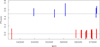 |
Fig. 1. Planetary phases observed as a function of MJD. Phases of the primary and secondary transits are marked by horizontal lines for sake of clarity. |
The five observations carried with the Medium filter were acquired in FullWindow mode (field of view ∼35′), while the remaining 20 observations that used the Thin1 filter were obtained in SmallWindow mode, where only a fraction of the chips were used to imaging the region around the target. The faster timing allowed by the SmallWindow mode reduces pile-up effects, however this is irrelevant in the case of HD 189733 A, since the source count rate is not exceptionally high (as compared to other very bright astrophysical sources).
The datasets were downloaded from the XMM-Newton web archive1 and reduced with SAS v18.0 in order to obtain tables of events calibrated in sky and detector positions, arrival times, pulse energies, and quality grades. The selection of events and their filtering in appropriate energy bands and quality grade has been performed through the SAS task EVSELECT. The same task allows us to accumulate light curves and spectra for the EPIC datasets.
A circular region of a 30″ radius used to extract the events associated with an X-ray source imaged with XMM-Newton-pn contains about 80% of the total events emitted by the source. HD 189733 has two nearby X-ray sources within about 12″: the M type star HD 189733 B, and an X-ray source that is likely of extra-galactic nature and perhaps associated with an AGN (hereafter source C) (Pillitteri et al. 2010; Poppenhaeger et al. 2013). Figure 2 shows the positions in one of the MOS1 images. We display here the MOS because allows for a better resolution over the pn. For the analysis of light curves and spectra, we used the data from pn because they offer a higher count statistics over MOS. The contribution of events from these sources to the light curves and spectra of HD 189733 A must thus be taken into account. For HD 189733 B and source C we extracted the events and light curves in two 5″ regions around their centroids. Source C has a hard spectrum (Pillitteri et al. 2010, 2011) and, from an examination of its light curves, it does not seem to vary significantly in time. These two conditions allow us to minimize the contamination from source C by simply restricting our analysis to the band 0.3−2.0 keV and excising the core of the counts centroid up to 8″. Previous analyses of the X-ray spectra of HD 189733 A have demonstrated that most of the coronal emission of HD 189733 A is concentrated at energies below 1 keV (Pillitteri et al. 2014).
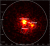 |
Fig. 2. MOS1 image of HD 189733 during observation 0744981201. The brightest source is HD 189733 A, followed by HD 189733 B and source C (likely a background AGN). The circles indicate regions of size 5″. The large circle has radius 30″. HD 189733 B was flaring during this observation while during quiescence was barely detected. |
The operative way to minimize the contamination of the light curves of HD 189733 A is thus summarized as follows:
-
(i) select pn events in a 30″ region centered on HD 189733 A and in the band 0.3–2.0 keV;
-
(ii) exclude the events in two 8″ circular regions centered on the positions of HD 189733 B and source C;
-
(iii) select the events in a semi-circular region opposite; to and not encompassing the positions of HD 189733 B and source C. This is a control set for the variability of HD 189733 B, (cf. Fig. 3);
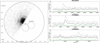
Fig. 3. Discriminating among different sources of variability. Left panel: pn image and selection of events of HD 189733 A in a semicircular region during observation 0744981201 in the band 0.3–2.0 keV. The circles indicate regions of size 5″. The large circle has radius 30″. Right panel: three examples of light curves where flaring of HD 189733 A or HD 189733 B is detected. The gray light curves are from events in a 30″ region minus two 8″ regions around HD 189733 B and source C (selection i + ii ). The time bins are 600 s each. The black light curves are accumulated from the events in the semicircular region opposite to HD 189733 B and source C as the figure in the left panel. Green light curves are made from the events of HD 189733 B in two 5″ regions. The background light curves scaled to the area of selection i + ii are also shown. In the top panel, a flare is visible both in the gray and green curves, but not in the black curve; this allows us to conclude that the flaring source was HD 189733 B and contaminated the selection in i + ii but not the selection in the semicircular region on the opposite side. In the middle panel, a flare is detected both in gray and black curves, this flare is genuinely due to HD 189733 A. In the bottom panel three flares are detected, the first one, seen in gray and black curves, attributed to HD 189733 A; while the second one is visible in gray and green curves and attributed to HD 189733 B. Another small flare of HD 189733 A is visible after the flare of HD 189733 B.
-
(iv) select events from a 40″ circular region for background subtraction to be applied to the light curves obtained in ii and iii.
Light curves with binning of 600 s obtained from events selected at points i and ii have been used for the analysis of variability of HD 189733 A and HD 189733 B, respectively. The choice of the binning interval is justified by the subsequent use of an algorithm to detect variability and flares, which assumes that in each bin, the counts follow an underlying Gaussian distribution (see Sect. 3.2.2). A bin of 600 s gives on average about 100–150 counts per bin, which fulfills the requirement of Gaussianity for all the observations, even during quiescent phases. When HD 189733 B was quiescent, its flux was very low and similar to the local background flux. However, in the case of flares from HD 189733 B, the light curves of HD 189733 A obtained at i+ii also show an excess due to the flares from HD 189733 B. The flux of HD 189733 B can overwhelm the flux of HD 189733 A at the position of the centroid of HD 189733 A even when excising the events in a 8″ region as in ii. Hence, the flares of HD 189733 B can be mistakenly attributed to HD 189733 A. To check any flaring of HD 189733 B we used the light curves obtained in point iii in order to determine the intervals with flares from HD 189733 B in the light curves obtained from points i+ii. The light curves of the events in a semicircular region of 30″ not comprising HD 189733 B and source C (point iii) served as a control sample to be compared to the light curves obtained at points i and ii. Figure 3 shows both the selection region in i through iii, along with three examples where the light curves of the primary are contaminated by flares of the secondary.
While the background can be variable in our XMM-Newton observations, we did not remove high background intervals. We preferred to keep uninterrupted time series within each observation and subtract the scaled background count rates to obtain the net source count rates. However, we did not consider the intervals of strong background variability for the subsequent analysis of flares (see Sect. 3).
3. Results
Here, we introduce the variability analysis of HD 189733 B and the variability of HD 189733 A.
3.1. Flares of the M star HD 189733 B
As mentioned in the introduction, HD 189733 B is a M4 star with a relatively low level of quiescent emission, We identified the flares by eye as the main episodes of variability, characterized by a steep rise followed by a slower decay. We thus identified four bright flares from HD 189733 B in the 25 XMM-Newton observations. In the remaining 21 observations, HD 189733 B was quiescent and its flux was barely in excess with respect to the background level.
Figure 4 shows the four pn light curves during which HD 189733 B was flaring. The flare in ObsId 0744980201 is heavily affected by background variability, so we do not discuss it in detail here. Its duration was about 5 ks with a rise time of about 900−1200 s, the peak intensity was about a factor of four with respect to the quiescent rate, and it is the faintest among the flares detected in HD 189733 B.
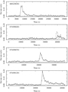 |
Fig. 4. pn light curves of HD 189733 B with flares. The time bins are 600 s. The light curves of the star (black curve) and the scaled background (gray curve) are shown. |
During observation 0744981201, we observed the brightest flare from HD 189733 B, with a ratio of the peak-to-quiescent rate equal to ∼30. The rise phase of the flare was about 1200 ± 300 s. The decay phase is characterized by an initial steep decrease of duration of about 8000 s (e-folding time ∼3500 s), followed by a much flatter decay that covers the remaining exposure time (about 16 ks). The star did not return to its initial quiescent rate, rather it kept emitting a flux about 3.5 times higher than the quiescent flux before the flare. Small impulses are visible during this post-flare phase – this flickering perhaps occurred in the same coronal region after the main ignition resulting thus in an overall flux higher than before the flare.
Flares detected in ObsIds 0692290301 and 0744980701 are very similar, with rise times tr ∼ 1200−1500 s and decay encompassing about 5000 s. The flare in ObsId 0692290301 has been cited in Bourrier et al. (2020). These two flares were less bright than the flare in 0744981201, reaching a peak rate of 28 and 13 times the quiescent rate, respectively. All the three flares seem to show a secondary peak after the initial fast decay hinting a second ignition or a triggered ignition in nearby coronal loops after the first event.
The spectra of the quiescent phases are well described with a thermal component at 0.3 ± 0.1 keV with a flux of 4−6 × 10⁻¹⁴ erg s−1 cm−2 in 0.3−2.0 keV band corresponding to a luminosity of 2−3 × 1027 erg s−1. These values are a factor of four to five higher than the X-ray luminosity derived by Poppenhaeger et al. (2013) with Chandra. During the flares a second thermal component is found at 1.3−1.5 keV in addition to the cool one. The flux rises by a factor of 10 or more and the luminosity reaches ∼3 × 1028 erg s−1. Using some diagnostics based on peak temperatures and decay time (Serio et al. 1991; Reale 2007), we can infer flaring loop sizes of order of 5 × 1010 cm, which is comparable to the radius of the star. The shape and temperatures of these flares resemble those observed in the Sun and other solar analogs that are due to mechanisms of coronal heating and are related to magnetic reconnection. The energy released by these flares is of order of 1.2−1.4 × 1032 erg and the cumulative energy is more than 4 × 1032 erg released on a total exposure time of 958 ks. Two of these flares were observed four days apart (ObsId 0744980701 and 0744981201). We speculate that they could have been originated in the same region – one that is more active than the rest of the corona.
3.2. Emission and variability of HD 189733 A
3.2.1. Hardness ratio and mean coronal temperature of HD 189733 A
We constructed the light curves of HD 189733 A in 0.3–1.0 keV and 1.0–2.0 keV bands with binnings of 600 s in order to calculate an hardness ratio (HR: (H − S)/(H + S)) (Fig. B.1). From the HR values we derived a mean coronal temperature of the star by means of a library of synthetic spectra calculated with XSPEC software. The spectra were modeled with a single thermal APEC component with temperatures in a range between 0.1 and 2.0 keV. From the synthetic spectra convolved with the spectral response and effective area of XMM-Newtonpn, we derived counts and HRs in the bands 0.3−1.0 keV (soft) and 1.0−2.0 keV (hard) as for the real data. We used the effective area files calculated for the Thin1 and the Medium filters and used the appropriate set of simulated spectra for each observation to calculate the expected HR values corresponding to each value of kT of the spectra. Then we interpolated the simulated HRs onto the observed HRs to obtain the corresponding values of kT. Figure 5 shows the values of HR during the 25 observations as well as the relationship between HR and kT of the model and the values of temperatures as a function of the XMM-Newton exposure time. The differences between the Thin1 and Medium filters are minimal (less than 1%). The intervals where the flares of HD 189733 B occurred were removed from the analysis. The kT light curve indicates that almost all the coronal emission of HD 189733 A is always below 1 keV. The relationship between HR and kT becomes insensitive for temperature above 1.4 keV but it works well for HD 189733 A because of the softness of its spectrum. Overall, we do not recognize cyclic variations of the hardness of the coronal spectrum of HD 189733 A over a timescale of eight years or fewer, which could arise from an activity cycle on such a timescale.
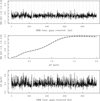 |
Fig. 5. Hardness ratio and coronal temperature. Top panel: time series of the hardness ratio (HR) calculated in the bands 0.3−1.0 keV (soft) and 1.0−2.0 keV (hard) as a function of the exposure time (bins of 600 s). Vertical lines indicate the durations of each XMM-Newton observation. The average uncertainty of HR is about 0.09 (quantile range 25%–75%: 0.08–0.11). Middle panel: relationship between HR and temperature (kT) derived with a library of synthetic spectra and XSPEC software for the case of Thin1 filter (solid line) and Medium filter (dashed line). Bottom panel: Time series of kT expressed in keV (average uncertainty is 0.09 keV, range 25%–75%: 0.07–0.12 keV). |
Figure 6 shows the histogram of the values of the mean temperatures (kT) of the corona of HD 189733 A derived from HR. The distribution of kT has a median of 0.4 keV corresponding to about 4.4 MK, the 25%−75% quantile range is in 0.3−0.5 keV and the maximum temperature is ∼0.9 keV (10.8 MK).
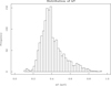 |
Fig. 6. Histogram of the values of the mean temperature (kT) inferred from the hardness ratio values. |
From the count rates and the mean coronal kT derived from HR, we obtained fluxes and luminosities by adopting a conversion factor (CF) between count rates and fluxes in the 0.3–2.0 keV band. We used PIMMS to convert pnThin1 (Medium) filter count rates to fluxes with a grid of optically thin plasma thermal APEC models spanning kT in 0.1–1.2 keV. We set NH = 0 cm−2 as this is compatible with the gas absorption measured from the spectra of HD 189733 A and its nearby distance (Pillitteri et al. 2010), and the overall metal abundance was chosen equal to Z = Z⊙ 2. We thus derived a relationship between kT and CF for observations made with either Thin1 or Medium filters. The CF values range between 1.08 × 10⁻¹² and 1.31 × 10⁻¹² erg cnt−1 cm−2. We interpolated these relationships to obtain the CFs for each time bin of each observation and relative to Thin1 or Medium filter. We also corrected the count rates for systematic offsets like the fraction of PSF comprised in the extraction region of the events and dead time due to the read out of the frames with the SAS task epiclcorr. From the fluxes, we finally obtained luminosities, assuming a distance of 19.775 pc (plx = 50.57 ± 0.03 mas, Gaia Collaboration 2020). A synoptic view of the X-ray luminosity for all the XMM-Newton observations is given in Fig. B.3.
3.2.2. Flares of HD 189733 A
Once we identified the main flares of HD 189733 B, we went on to identify the flares of HD 189733 A. We first discarded the four time intervals where HD 189733 B was flaring and thus the predominant source of variability in the light curves. For identifying the flares of HD 189733 A and their lengths, we adopted a semi automatic method. We first determined a quiescent rate for each light curve corresponding to the 10% quantile of the distribution of the count rates in that curve. This approach excludes the bins where the count rate drops to low values due to telemetry issues (as in observation 2 of Fig. B.2 at ∼23 ks). The median quiescent luminosity of HD 189733 A in the 0.3 − |2.0 keV band is about 4.5 × 1027 erg s−1 (25%−75% range 4.3−5.3 × 1027 erg s−1).
We used the ChangePoint package (version 2.2.2) within R language (Killick & Eckley 2014) to detect changes of the count rates and to segment the light curves in intervals of statistically constant count rates. In our case we applied the ChangePoint package with the PELT algorithm to the background subtracted count rates of HD 189733 A and to the light curves of the background. The penalty parameter (p) is crucial for a coarser or finer segmentation of the light curve and needs to be properly set. A higher p results in fewer time segments, while a lower p produces more segments. The optimal value of p = 0.006 was assessed with a set of simulations of a constant source with count rates normally distributed around a mean value (rq), equal to the quiescent count rates that we determined in each light curve and with standard deviation (σq) equal to the median of the errors of the net count rates (after propagating the errors due to background subtraction). Thus, a value of p was chosen such that ChangePoint detects at most one break per light curve on average under the expectation that a constant (noisy) count rate produces only one time segment equal to the full exposure.
As explained in Sect. 2, the bin size of light curves was chosen in a way to guarantee enough counts per bin. We tested the use of smaller bin sizes of 100 s and 300 s with Changepoint. The results were that such finer binning produced a few more short time segments due to noise without additional information on the variability.
Using simulated light curves, we quantified also the sensitivity to small flares that could be confused with small statistical variability and were thus not detected. To do so, we injected a number of flares in the light curves of constant source described above. The flare profile was modeled with two exponentials for the rise and the decay phases. The analytical form is:
where t0 sets the time of the peak, τr and τd are the typical rise and decay times, respectively, and P is the peak normalization. To reduce the parameter space, we chose 1 ks for the rise time and 5 ks for the decay time. These values are reasonable choices that match well the observed characteristic rise and decay phases. The only free parameters of the flare model were thus the time of the peak (t0) and intensity of the peak (P) in units of sigma (σq).
The number of flares to inject was determined from a power law relationship dN/dE/day ∝ E−2 (see Sect. 4). We simulated flares with energies between 2 × 1030 − 1.2 × 1031 erg, which is the range where we observe a flattening of the flare distribution (cf. Fig. 8) and that corresponds to peaks in the range 0.5−1σq above the quiescent rates. The expected number of flares per day in this range of energy is about 16. We scaled this number for the duration of each observation and, thus, the number of injected flares was 5–11, depending on the length of each light curve. The ChangePoint algorithm applied to the simulated light curves resulted in about three time segments per light curve due to small flares detected at the penalty threshold chosen for the real data. These elevated segments are generated from a single flare or, more frequently, from the blend of several small flares.
Once we identified the time segments with ChangePoint, we grouped them into flares defined as the union of contiguous segments starting with a rising or a peaking segment and followed by one or more decay segments. In observation no. 2, the dip during the decay is due to a telemetry glitch; in this case, we considered the decay lasting from peak to the end of the observation. A reference level is given by the quiescent rate, rq, defined above. In some cases, the average rate is significantly above the quiescent level in a block more than 5 ks long, but it cannot be clearly associated to a single flare. In these cases, we checked whether the flickering could be due to blended small flares, as has been observed in several simulations. In those cases, and only when the average count rate in one block was higher than 1σq above the quiescent level rq, we tried to identify small flares subdividing the elevated interval into small ones. As a guidance, we checked the HR that tends to increase during the flares because of plasma heating. We applied the ChangePoint algorithm to the background curves as well and we discarded the time intervals when the background was very high from searching for flares (see Fig. B.2)
The number of flares identified in this way was 60 – with 47 occurring in observations taken around primary transits of HD 189733 Ab and another 13 occurring in observations taken at secondary transits. The rates of flares per ks were very similar: 0.063 ± 0.008 ks−1 for the total sample, 0.065 ± 0.01 ks−1 for the observations at primary transits and 0.054 ± 0.015 ks−1 for the observations at secondary transits. The rates of flares per day were 5.4 ± 0.7d−1, 5.7 ± 0.8d−1, 4.7 ± 1.3, respectively, for the full sample and the two sub-samples observed at the primary and secondary transits.
We multiplied the flares luminosities for each bin time (600 s) after subtracting the quiescent level and summed the energies per bin to obtain the total flare energies. In the next section, we discuss the properties of the flares, their energies, and the comparison between them and the flares observed in the Sun and solar type stars.
During transits, the planet could obscure a surface spot onto the star with projected size similar to that of the planet. Indeed, the available TESS light curve shows that some of the profiles of the optical transits are distorted due to the planet passing over a stellar spot (Colombo, priv. comm.). Moreover, it seems that the same spot lasted for more than one orbital period (∼2.2 days), so that the planet could have passed in front of the same region more than once. Photospheric spots are the anchors of magnetic loops and coronal active regions. The time required for the planet to transit across an active region of the size of Jupiter is about 1000 s. The possibility that the obscured region would flare during that interval and that the same flare would be unnoticed is, however, reputed to be low. Given the count statistics of the X-ray light curves and the chosen bin time, the event is hardly detectable with a high significance. Moreover, the patchy and variable stellar surface in X-rays makes these kinds of obscuration even less detectable.
4. Discussion and conclusions
In this paper, we analyze, in a homogeneous way, 25 observations of the HD 189733 system obtained with XMM-Newton between the years 2007–2015. This set of observations is quite unique in the context of stars hosting planets because they accumulated almost 1 Ms, devoted to observations of the same star in X-ray at two opposite phases of the orbit of its planet. The present study offers thus a comprehensive characterization of the variability across the lifetime of eight years for HD 189733 A.
In Table A.1, we report the list of identified flares with their duration, energy, total luminosity, and flux. We also report the flux received at the surface of HD 189733 Ab. When considering all the flares, the total flaring time was 423.6 ks out of 958 ks for a flare percentage of 44% of the exposure time. The total time of the flares that occurred around the secondary transits amounts to about 123.6 ks or ≈51.5% of the observing time (240 ks). The corresponding time at the primary transits was 300 ks or 41.8% of the observing time (718 ks). In the observed range of flare energies, the flares detected at secondary transits are more frequent than the flares detected at primary transits.
The range of flare energies spans about 1.2 orders of magnitude between log LX ≈ 30.6 erg and log LX ≈ 32.2 erg. The medians of flare energies observed around primary and secondary transits are slightly different (log EX ≈ 31.31 and 31.58, respectively) but the ranges of energies are similar in both sub-samples. A Kolmogorov-Smirnoff test applied to the two samples indicates a probability of ∼13% that the energies of flares seen at the secondary transit are drawn from the same underlying distribution of energies of flares detected at the primary transits. From this, we conclude that there is a slight, but not statistically significant hint that flares at the secondary transits were more energetic. In Fig. 7, we show the empirical cumulative distribution functions (ECDFs) of the two samples of flare energies. The greatest difference between the two ECDFs is seen at log E ≈ 31.6. The peak luminosities and the duration of the flares of the two samples do not show a trend, meaning that it is likely a combination of flares duration and peak luminosities to result in the slight difference of energies.
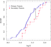 |
Fig. 7. Empirical cumulative distribution functions (ECDFs) of the energies of flares detected around primary and secondary transits. The arrow marks the largest separation between the two ECDFs at log E ≈ 31.63. |
Figure 8 shows the rate of flares per day with energies above a given threshold for the total sample, the flares detected near the planetary transits and those detected near or after the secondary transits. The frequency of X-ray flares with respect to their energies in the Sun and in Main Sequence stars is well described by a power law relationship:
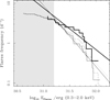 |
Fig. 8. Cumulative distributions of flares per day with energies above a given threshold (log N(E > E0)). Dashed line indicates the full sample of flares (Nflares = 60); thin solid line is relative to the flares observed at planetary transits (Nflares = 47); thick solid line is relative to the flares observed at secondary transits (Nflares = 13). The lines refer to a linear fit of each sample in the form log N(EX > E0)∝βlog EX. The range with energies log EX < 31.2 not used for the fit to the slopes is shaded in gray color. |

where the index α is of order of 2 (Hudson 1991; Kashyap et al. 2002; Drake et al. 2013). The log-log distribution shown in Fig. 8 allows us to estimate the slope γ of the linear relationship between the number of flares and their energies:

with the slope γ being related to α by the relationship γ = 1 − α.
The bias due to completeness of unidentified small flares makes the curves in Fig. 8 flatten below a given threshold (Eth). The value of Eth depends on the sensitivity of the instruments and the intensity of the flares. Above Eth the cumulative distribution is deemed complete and not affected by unidentified smaller flares, thus, it is possible to fit the tail of the distribution without any completeness bias. We calculated the slope at different energy thresholds and checked that for values log EX > 31.2, the slope does not change significantly. We thus considered only the 43/60 flares with energies above log Eth = 31.2 that roughly correspond to flares with peak luminosities between 5 × 1027 and 2.8 × 1028 erg s−1 or about one to six times the quiescent luminosities. In Sect. 3, we gave a statistical estimate of the number of small flares we could have missed. Their number amounts to about seven per light curve and 175 for the total observation time (11.1 days), or about ten small flares per day with energies 30.5 < log E < 31.2. However, in the case of a larger power law index α ∼ −2.5, the number of undetected small flares with 30.5 < log E < 31.2 can be up to 40 per day. In principle, our simulation of injected flares could be used to retrieve the completeness limit as a function of the flares energy. However, the flare model depends on a few choices we made about the shape and the rise and decay characteristic times, which we kept fixed to reduce the space parameter. The flare energies were obtained from the integration of the flare profiles, but any given value of total energy could correspond to flares with different profiles and duration. For this reason, we preferred to infer the completeness limit directly from the data.
For the full sample of flares, we obtained: α ∼ 2.45 ± 0.06; for the flares observed around the primary transits: α ∼ 2.53 ± 0.05; and for the flares observed at the secondary transit phases: α ∼ 2.04 ± 0.14. Overall, the modeling of the distribution of flare energies with a power law is a good approximation, however, the index of the power law that we find for HD 189733 A is steeper than the analog power law indices found is the Sun and in other solar-type stars.
The subsample of flares detected at the secondary transits shows a flatter energy distribution than the corresponding distribution at the primary transits. The respective power law indices differs by about 2−3σ, although the uncertainties in the slopes could be underestimated given the correlation of the errors among the bins.
We go on to consider whether the flares observed in HD 189733 A could be associated with coronal mass ejections (CMEs). For the Sun, Yashiro et al. (2004) observed that flares of classes higher than X2 (corresponding to fluxes of 0.2 erg s−1 cm−2) are always associated with CMEs. We calculated the average luminosities (0.3−2.0 keV) during flares and converted these to the GOES band (1−8 Å), with a scaling factor calculated assuming an APEC model with kT = 0.86 keV, which is appropriate for the peak temperatures we inferred from HR, assuming NH = 0 cm−2 and Z = Z⊙. The scaling factor was thus 0.1122. From the luminosities, we derived the fluxes at 1 AU and compared these to the GOES scale. Using Yashiro’s classification, a hypothetical Earth around HD 189733 A would have experienced flares of classes between X1 and X20, more than 70% of them associated with CMEs.
Drake et al. (2013) give an estimate of the mass rate of CMEs as a function of the GOES luminosity. The average luminosities of the flares of HD 189733 A converted in the GOES band give values above 6 × 1028 erg. From Fig. 3 in Drake et al. (2013), we infer that the mass rates ejected in the supposed CMEs are in excess of 10−12 M⊙ yr−1, with most of them peaking at 10−11 M⊙ yr−1 and reaching up to 10−10 M⊙ yr−1 in the most powerful flares, or about 6−600 × 1013 g s−1. Drake et al. (2013) give also the relationship between X-ray luminosity of flares and kinetic energy loss rate of the CME. From the flare luminosities of HD 189733 A, we infer a kinetic energy in excess of 10−4 L⊙ and a velocity of vCME ≈ 1000 km s−1.
Since the average X-ray activity of the stars declines with age, it is expected that also the most energetic flares become less frequent (see Johnstone et al. 2021). Audard et al. (2000) derived an empirical relationship between the number of flares per day with energies above 1032 erg and the average X-ray luminosities of the stars in the band 0.01–10 keV. After converting the luminosities in 0.0–10 keV, we detected five flares with energies above 1032 erg in 11.1 days or N(E > 1032 erg) ≈ 0.45 d−1 flares. The relationship described by Audard et al. (2000) for an average luminosity of HD 189733 A of 6 × 1028 erg s−1 predicts about 0.46 flares per day, which is perfectly matched with the observed rate. Two out of the five flares with E > 1032 erg were detected at secondary transits, again hinting that energetic flares occur preferentially at those phases. The finding that more energetic flares occur more frequently after the planetary eclipse is in agreement with prior results (Pillitteri et al. 2011, 2015). The reason for this could be some kind of star-planet interaction due to the escaping planetary gas trapped in the global magnetic field around the star. The interplay between ionized gas and magnetic field could generate reconnection events leading to energetic flares (cf. Cohen et al. 2011). In support of this scenario, the analysis of the flare observed in ObsID 0690890201 (Pillitteri et al. 2014) led us to conclude that the flaring structure had a size of a few stellar radii, which is compatible with a magnetic structure elongated towards the planet – produced by the dynamics of the ionized gas escaping the planet and launched towards the star (Colombo et al. 2021, see also the MHD modeling in Matsakos et al. 2015). Using Eq. (14) of Serio et al. (1991) and by assuming a typical decay time τd = 5 ks and a peak temperature of 0.9 keV, we estimated an average loop length of ≈1.6 stellar radii. For longer lasting flares with τd ∼ 10 ks, the loop would be twice in length with the top of the loop distant about 1 stellar radius above the stellar surface. HD 189733 was one of the first cases for which star-planet interaction was suggested from the varying emission of Ca II H&K lines (Shkolnik et al. 2008). Pillitteri et al. (2014) derived a loop length of about four stellar radii from the analysis of an oscillatory pattern detected in a flare light curve. The height of this loop was close to 25% of the separation between the planet and the star and it is above the star’s co-rotation radius. The latter indicates there is a mechanism that maintained the loop stable. The authors suggested that the star and the planet are magnetically connected. This hypothesis was later supported by MHD simulations and FUV observations (Matsakos et al. 2015; Pillitteri et al. 2015). The latter authors speculated that the star could accrete gas evaporating from the planet. The impact of the stream onto the stellar surface would cause a hot spot that is approximately 90 degrees ahead of the sub-planetary point. Pillitteri et al. (2015) also showed that the star exhibited FUV variability in phase with the planet motion. The hot spot would become visible during the secondary transit and be hidden to the observer during the primary transit. The stellar activity in the hot spot is higher in terms of flare occurrence and intensity but does not cause a perceptible enhancement in the quiescent emission of the star, possibly due to the reduced extension of the spot. Further MHD simulations show that the stream from the planet to the star is dynamically varying due to the interaction with the stellar wind (Colombo et al. 2021). In a concurrent scenario (not necessarily an alternative to the first one), the magnetized environment between the planet and the star traps the out-flowing ionized gas from HD 189733Ab, but the planetary orbital motion stretches the resulting magnetic field and triggers the flares (cf. Lanza 2013). These speculations are, however, biased by the fact that we have observed a relatively narrow portion of planetary orbital phases and that a continuous and repeated monitoring covering at least half orbit between the two opposite phases has not been obtained. Further monitoring at the secondary transit phases is desirable to match the unbalanced exposure times at the two opposite phases and to better determine any difference of flare energies when the planet is facing the two different sides of the star.
The average temperature of the corona of HD 189733A is estimated at around 0.4 keV (10%–90% range in 0.27–0.58 keV). It is only during flares that the temperature rises up to about 0.9 keV. The flares observed near primary transits and those observed at secondary transits show similar temperatures. The lack of temperatures in excess of 1 keV is not due to a lack of sensitivity of our analysis (which can, in principle, detect temperatures up to ∼1.5 keV). The corona of HD 189733 A remained relatively cold even during the most energetic flares, while, for example, HD 189733 B showed temperatures on the order of 1.3−1.5 keV during the four flares that we observed and that released energies E ≈ 1032 erg.
From the monitoring of chromospheric lines as activity indicators and in X-ray, a number of stars are known to possess activity cycles even among planet host stars. The ubiquity of such cycles are not established and depends on several factors such as the stellar age. Saar & Brandenburg (1999) and Böhm-Vitense (2007) showed that when comparing rotational periods with the lengths of activity cycles, stars can be divided into two sequences: a steeper sequence formed by young and active stars and a flatter sequence of inactive and older stars. The Sun fits in between the two sequences. HD 189733 A does not seem to possess an X-ray activity cycle, at least when considering a timescale of eight years. HD 189733 A has a rotational period of 11.7 days, as an active star (mimicking an age of less than 1 Gyr), it belongs to the steep sequence of active and young stars and, thus, it would have an activity cycle of ≥12 years.
One peculiar behavior characterizing HD 189733 A is the fact that its variability in X-rays is totally different from the variability in the optical band. TESS observed HD 189733 A (TIC 256364928) during sector 41 for about 27 days and about 11 transits were recorded. The TESS light curve does not clearly show short timescale variability due to flares. As remarked in Sect. 3, the planet obscured some surface spots but yet the star was relatively inactive, behaving instead like an old quiet star in spite of its level of X-ray activity and luminosity. We speculate that the stark difference between the activity and the relatively cold flares observed in X-rays and the optical band could be related to the angular momentum transfer from the planet to the star and its influence on the mechanism of magnetic dynamo that produces the corona. Furthermore, the magnetic interaction between the star and the planet could produce a significant part of the observed X-ray emission and variability. Lanza (2013) quantifies the power emitted by two possible mechanisms of loop stretching due to magnetic interaction of the star+planet magnetospheres or of magnetic loops anchored between a star and its hot Jupiter. In particular, the second mechanism could easily produce a power of order of 1028 erg s−1 (similar to the average X-ray luminosity of HD 189733 A) for a planetary magnetic field of ∼3 G at the pole and separation equal to that of HD 189733 Ab.
We analyzed the variability of HD 189733 B, taking into account the close angular separation with the primary HD 189733 A in order to carefully distinguish its time variability in X-ray. This mainly consisted of four bright flares detected in 958 ks, which correspond to a rate of one flare every 2.8 days. On average, the flares released energies in excess of 1032 erg. The quiescent luminosity of HD 189733 B is about log LX ∼ 27.27 in 0.3−2.0 keV, which is about a factor four higher than found in Chandra observations (Poppenhaeger et al. 2013). The luminosity is still consistent with that of a dM star with an age of a it is Gyr; however, in contrast to the age that would otherwise be inferred from the X-ray activity of HD 189733 A, which is less than 1 Gyr. The age discrepancy between the two components of the HD 189733 system has been discussed in literature and explained as the result of spin up on the part of the star with the hot Jupiter, accompanied by the transfer of angular momentum from the orbital motion of the planet to the rotation of the star (Pillitteri et al. 2010; Poppenhaeger & Wolk 2014). The flare temperatures of HD 189733 B were in excess of 1.3 keV – in stark contrast to the flare temperatures of the flares of HD 189733 A, which remained below 1 keV.
This choice is supported by the results of the best fit of the full exposure spectrum of observation nr. 15 where there was negligible flaring activity. From a best fit to a model with two thermal APEC components we obtained (90% confidence ranges quoted in braces): kT1 = 0.25 (0.22−0.28) keV, kT2 = 0.8 (0.76−0.91) keV, and Z = 0.15 Z⊙ (0.11−0.19).
Acknowledgments
The authors acknowledge the anonymous referee for their useful comments and suggestions. I.P., A.M. and G.M. acknowledge financial support from the ASI-INAF agreement n.2018-16-HH.0, and from the ARIEL ASI-INAF agreement n.2021-5-HH.0. Based on observations obtained with XMM-Newton, an ESA science mission with instruments and contributions directly funded by ESA Member States and NASA.
References
- Audard, M., Güdel, M., Drake, J. J., & Kashyap, V. L. 2000, ApJ, 541, 396 [Google Scholar]
- Bakos, G. Á., Pál, A., Latham, D. W., Noyes, R. W., & Stefanik, R. P. 2006, ApJ, 641, L57 [NASA ADS] [CrossRef] [Google Scholar]
- Böhm-Vitense, E. 2007, ApJ, 657, 486 [CrossRef] [Google Scholar]
- Borucki, W. J., Koch, D., Basri, G., et al. 2006, ISSI Sci. Rep. Ser., 6, 207 [NASA ADS] [Google Scholar]
- Bouchy, F., Udry, S., Mayor, M., et al. 2005, A&A, 444, L15 [EDP Sciences] [Google Scholar]
- Bourrier, V., Lecavelier des Etangs, A., Dupuy, H., et al. 2013, A&A, 551, A63 [NASA ADS] [CrossRef] [EDP Sciences] [Google Scholar]
- Bourrier, V., Wheatley, P. J., Lecavelier des Etangs, A., et al. 2020, MNRAS, 493, 559 [Google Scholar]
- Cecchi-Pestellini, C., Ciaravella, A., Micela, G., & Penz, T. 2009, A&A, 496, 863 [NASA ADS] [CrossRef] [EDP Sciences] [Google Scholar]
- Cohen, O., Kashyap, V. L., Drake, J. J., et al. 2011, ApJ, 733, 67 [NASA ADS] [CrossRef] [Google Scholar]
- Colombo, S., Pillitteri, I., Orlando, S., & Micela, G. 2021, ArXiv e-prints [arXiv:2111.11110] [Google Scholar]
- Drake, J. J., Cohen, O., Yashiro, S., & Gopalswamy, N. 2013, ApJ, 764, 170 [NASA ADS] [CrossRef] [Google Scholar]
- Gaia Collaboration 2020, VizieR Online Data Catalog: I/350 [Google Scholar]
- Gardner, J. P., Mather, J. C., Clampin, M., et al. 2006, Space Sci. Rev., 123, 485 [Google Scholar]
- Hudson, H. S. 1991, Sol. Phys., 133, 357 [Google Scholar]
- Johnstone, C. P., Bartel, M., & Güdel, M. 2021, A&A, 649, A96 [EDP Sciences] [Google Scholar]
- Kashyap, V. L., Drake, J. J., Güdel, M., & Audard, M. 2002, ApJ, 580, 1118 [Google Scholar]
- Killick, R., & Eckley, I. A. 2014, J. Stat. Softw., 58, 1 [CrossRef] [Google Scholar]
- Kubyshkina, D., Fossati, L., Erkaev, N. V., et al. 2018, ApJ, 866, L18 [NASA ADS] [CrossRef] [Google Scholar]
- Lanza, A. F. 2013, A&A, 557, A31 [NASA ADS] [CrossRef] [EDP Sciences] [Google Scholar]
- Lecavelier des Etangs, A., Bourrier, V., Wheatley, P. J., et al. 2012, A&A, 543, L4 [NASA ADS] [CrossRef] [EDP Sciences] [Google Scholar]
- Locci, D., Petralia, A., Micela, G., et al. 2022, Planet. Sci., 3, 1 [NASA ADS] [CrossRef] [Google Scholar]
- Matsakos, T., Uribe, A., & Königl, A. 2015, A&A, 578, A6 [NASA ADS] [CrossRef] [EDP Sciences] [Google Scholar]
- Pillitteri, I., Wolk, S. J., Cohen, O., et al. 2010, ApJ, 722, 1216 [NASA ADS] [CrossRef] [Google Scholar]
- Pillitteri, I., Günther, H. M., Wolk, S. J., Kashyap, V. L., & Cohen, O. 2011, ApJ, 741, L18 [NASA ADS] [CrossRef] [Google Scholar]
- Pillitteri, I., Wolk, S. J., Lopez-Santiago, J., et al. 2014, ApJ, 785, 145 [NASA ADS] [CrossRef] [Google Scholar]
- Pillitteri, I., Maggio, A., Micela, G., et al. 2015, ApJ, 805, 52 [Google Scholar]
- Poppenhaeger, K., & Wolk, S. J. 2014, A&A, 565, L1 [NASA ADS] [CrossRef] [EDP Sciences] [Google Scholar]
- Poppenhaeger, K., Schmitt, J. H. M. M., & Wolk, S. J. 2013, ApJ, 773, 62 [Google Scholar]
- Reale, F. 2007, A&A, 471, 271 [NASA ADS] [CrossRef] [EDP Sciences] [Google Scholar]
- Ricker, G. R., Winn, J. N., Vanderspek, R., et al. 2015, J. Astron. Telesc. Instrum. Syst., 1, 014003 [Google Scholar]
- Saar, S. H., & Brandenburg, A. 1999, ApJ, 524, 295 [NASA ADS] [CrossRef] [Google Scholar]
- Serio, S., Reale, F., Jakimiec, J., Sylwester, B., & Sylwester, J. 1991, A&A, 241, 197 [NASA ADS] [Google Scholar]
- Shkolnik, E., Bohlender, D. A., Walker, G. A. H., & Collier Cameron, A. 2008, ApJ, 676, 628 [NASA ADS] [CrossRef] [Google Scholar]
- Tinetti, G., Drossart, P., Eccleston, P., et al. 2018, Exp. Astron., 46, 135 [NASA ADS] [CrossRef] [Google Scholar]
- Yashiro, S., Gopalswamy, N., Michalek, G., et al. 2004, J. Geophys. Res. (Space Phys.), 109, A07105 [NASA ADS] [CrossRef] [Google Scholar]
Appendix A: Table of flares
List of identified flares.
Appendix B: Light curves
"In this appendix, we display the HR light curves derived from the pn count rates in the bands 0.3-1.0 keV and 1.0 - 2.0 keV (Fig. B.1), the pn light curves of HD 189733 A (Fig. B.2) obtained in 25 XMM-Newton observations, and the light curves of the X-ray luminosity of HD 189733 A in the band 0.3 - 2.0 keV (Fig. B.3).
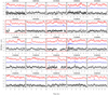 |
Fig. B.1. Solid black lines with error bars: light curves of hardness ratio of HD 189733 A obtained from pn events for each observation. Red and blue curves: Soft (0.3-1.0 keV) and hard (1.0-2.0) band light curves scaled between zero and the maximum of soft rate. As in Fig. B.2, the panels marked with a red border indicate observations where flares of HD 189733 B were detected. In these curves, we discarded the intervals relative to the flares of HD 189733 B. |
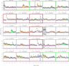 |
Fig. B.2. Light curves of HD 189733 A obtained with pn in the band 0.3−2.0 keV. The points with error bars are the net count rates of HD 189733 A for the events in the selection operated at points i and ii of Sect. 2. The horizontal red segments mark the intervals identified with the Changepoint algorithm. Similarly, the light red segments represent the intervals of constant background. In intervals of high background variability (gray shaded areas), we did not search for flares in HD 189733 A. The flares are shaded with different colors in each panel. The horizontal solid blue lines represent the quiescent rates and the ±1sigma range. Panels contoured with a green border refers to observations at the secondary transits. Panels marked with a red border indicate where variability of HD 189733 B was prominent. |
 |
Fig. B.3. Synoptic plot of the logarithm of the X-ray luminosity of HD 189733 A in the band 0.3-2.0 keV observed in the XMM-Newton observations. Gaps in the light curves correspond to intervals where flares from HD 189733 B affected the estimated of the count rate of HD 189733 A. |
All Tables
All Figures
|
Fig. 1. Planetary phases observed as a function of MJD. Phases of the primary and secondary transits are marked by horizontal lines for sake of clarity. |
| In the text | |
|
Fig. 2. MOS1 image of HD 189733 during observation 0744981201. The brightest source is HD 189733 A, followed by HD 189733 B and source C (likely a background AGN). The circles indicate regions of size 5″. The large circle has radius 30″. HD 189733 B was flaring during this observation while during quiescence was barely detected. |
| In the text | |
|
Fig. 3. Discriminating among different sources of variability. Left panel: pn image and selection of events of HD 189733 A in a semicircular region during observation 0744981201 in the band 0.3–2.0 keV. The circles indicate regions of size 5″. The large circle has radius 30″. Right panel: three examples of light curves where flaring of HD 189733 A or HD 189733 B is detected. The gray light curves are from events in a 30″ region minus two 8″ regions around HD 189733 B and source C (selection i + ii ). The time bins are 600 s each. The black light curves are accumulated from the events in the semicircular region opposite to HD 189733 B and source C as the figure in the left panel. Green light curves are made from the events of HD 189733 B in two 5″ regions. The background light curves scaled to the area of selection i + ii are also shown. In the top panel, a flare is visible both in the gray and green curves, but not in the black curve; this allows us to conclude that the flaring source was HD 189733 B and contaminated the selection in i + ii but not the selection in the semicircular region on the opposite side. In the middle panel, a flare is detected both in gray and black curves, this flare is genuinely due to HD 189733 A. In the bottom panel three flares are detected, the first one, seen in gray and black curves, attributed to HD 189733 A; while the second one is visible in gray and green curves and attributed to HD 189733 B. Another small flare of HD 189733 A is visible after the flare of HD 189733 B. |
| In the text | |
|
Fig. 4. pn light curves of HD 189733 B with flares. The time bins are 600 s. The light curves of the star (black curve) and the scaled background (gray curve) are shown. |
| In the text | |
|
Fig. 5. Hardness ratio and coronal temperature. Top panel: time series of the hardness ratio (HR) calculated in the bands 0.3−1.0 keV (soft) and 1.0−2.0 keV (hard) as a function of the exposure time (bins of 600 s). Vertical lines indicate the durations of each XMM-Newton observation. The average uncertainty of HR is about 0.09 (quantile range 25%–75%: 0.08–0.11). Middle panel: relationship between HR and temperature (kT) derived with a library of synthetic spectra and XSPEC software for the case of Thin1 filter (solid line) and Medium filter (dashed line). Bottom panel: Time series of kT expressed in keV (average uncertainty is 0.09 keV, range 25%–75%: 0.07–0.12 keV). |
| In the text | |
|
Fig. 6. Histogram of the values of the mean temperature (kT) inferred from the hardness ratio values. |
| In the text | |
|
Fig. 7. Empirical cumulative distribution functions (ECDFs) of the energies of flares detected around primary and secondary transits. The arrow marks the largest separation between the two ECDFs at log E ≈ 31.63. |
| In the text | |
|
Fig. 8. Cumulative distributions of flares per day with energies above a given threshold (log N(E > E0)). Dashed line indicates the full sample of flares (Nflares = 60); thin solid line is relative to the flares observed at planetary transits (Nflares = 47); thick solid line is relative to the flares observed at secondary transits (Nflares = 13). The lines refer to a linear fit of each sample in the form log N(EX > E0)∝βlog EX. The range with energies log EX < 31.2 not used for the fit to the slopes is shaded in gray color. |
| In the text | |
|
Fig. B.1. Solid black lines with error bars: light curves of hardness ratio of HD 189733 A obtained from pn events for each observation. Red and blue curves: Soft (0.3-1.0 keV) and hard (1.0-2.0) band light curves scaled between zero and the maximum of soft rate. As in Fig. B.2, the panels marked with a red border indicate observations where flares of HD 189733 B were detected. In these curves, we discarded the intervals relative to the flares of HD 189733 B. |
| In the text | |
|
Fig. B.2. Light curves of HD 189733 A obtained with pn in the band 0.3−2.0 keV. The points with error bars are the net count rates of HD 189733 A for the events in the selection operated at points i and ii of Sect. 2. The horizontal red segments mark the intervals identified with the Changepoint algorithm. Similarly, the light red segments represent the intervals of constant background. In intervals of high background variability (gray shaded areas), we did not search for flares in HD 189733 A. The flares are shaded with different colors in each panel. The horizontal solid blue lines represent the quiescent rates and the ±1sigma range. Panels contoured with a green border refers to observations at the secondary transits. Panels marked with a red border indicate where variability of HD 189733 B was prominent. |
| In the text | |
|
Fig. B.3. Synoptic plot of the logarithm of the X-ray luminosity of HD 189733 A in the band 0.3-2.0 keV observed in the XMM-Newton observations. Gaps in the light curves correspond to intervals where flares from HD 189733 B affected the estimated of the count rate of HD 189733 A. |
| In the text | |
Current usage metrics show cumulative count of Article Views (full-text article views including HTML views, PDF and ePub downloads, according to the available data) and Abstracts Views on Vision4Press platform.
Data correspond to usage on the plateform after 2015. The current usage metrics is available 48-96 hours after online publication and is updated daily on week days.
Initial download of the metrics may take a while.