| Issue |
A&A
Volume 659, March 2022
|
|
|---|---|---|
| Article Number | A153 | |
| Number of page(s) | 21 | |
| Section | Extragalactic astronomy | |
| DOI | https://doi.org/10.1051/0004-6361/202142440 | |
| Published online | 21 March 2022 | |
The multifarious ionization sources and disturbed kinematics of extraplanar gas in five low-mass galaxies
1
Space Physics and Astronomy research unit, University of Oulu, 90014 Oulu, Finland
e-mail: This email address is being protected from spambots. You need JavaScript enabled to view it.
2
Centre of Astrophysics Research, School of Physics, Astronomy and Mathematics, University of Hertfordshire, Hatfield AL10 9AB, UK
3
Departamento de Astrofísica, Universidad de La Laguna, 38200 La Laguna, Tenerife, Spain
4
Instituto de Astrofísica de Canarias, 38205 La Laguna, Tenerife, Spain
5
Department of Physics, Engineering Physics and Astrophysics, Queen’s University, Kingston, ON K7L 3N6, Canada
6
Finnish Centre of Astronomy with ESO (FINCA), Vesilinnantie 5, 20014 University of Turku, Finland
7
Specim, Spectral Imaging Ltd., Elektroniikkatie 13, 90590 Oulu, Finland
Received:
14
October
2021
Accepted:
13
December
2021
Abstract
Aims. We investigate the origin of the extraplanar diffuse ionized gas (eDIG) and its predominant ionization mechanisms in five nearby (17–46 Mpc) low-mass (109–1010 M⊙) edge-on disk galaxies: ESO 157-49, ESO 469-15, ESO 544-27, IC 217, and IC 1553.
Methods. We acquired Multi Unit Spectroscopic Explorer (MUSE) integral field spectroscopy and deep narrowband Hα imaging of our sample galaxies. To investigate the connection between in-plane star formation and eDIG, we measure the star formation rates (SFRs) and perform a photometric analysis of our narrowband Hα imaging. Using our MUSE data, we investigate the origin of eDIG via kinematics, specifically the rotation velocity lags. We also construct standard diagnostic diagrams and emission-line maps (EW(Hα), [N II]/Hα, [S II]//Hα, [O III]/Hβ) and search for regions consistent with ionization by hot low-mass evolved stars (HOLMES) and shocks.
Results. We measure eDIG scale heights of hzeDIG = 0.59−1.39 kpc and find a positive correlation between them and specific SFRs. In all galaxies, we also find a strong correlation between extraplanar and midplane radial Hα profiles. These correlations along with diagnostic diagrams suggest that OB stars are the primary driver of eDIG ionization. However, we find regions consistent with mixed OB–HOLMES and OB–shock ionization in all galaxies and conclude that both HOLMES and shocks may locally contribute to the ionization of eDIG to a significant degree. From Hα kinematics, we find rotation velocity lags above the midplane with values between 10 and 27 km s−1 kpc−1. While we do find hints of an accretion origin for the ionized gas in ESO 157–49, IC 217, and IC 1553, overall the ionized gas kinematics of our galaxies do not match a steady galaxy model or any simplistic model of accretion or internal origin for the gas.
Conclusions. Despite our galaxies’ similar structures and masses, our results support a surprisingly composite image of ionization mechanisms and a multifarious origin for the eDIG. Given this diversity, a complete understanding of eDIG will require larger samples and composite models that take many different ionization and formation mechanisms into account.
Key words: galaxies: ISM / galaxies: photometry / galaxies: kinematics and dynamics / galaxies: star formation
© ESO 2022
1. Introduction
Diffuse ionized gas (DIG) is a component of the interstellar medium (ISM), the non-stellar baryonic component of galaxies. This extensive, warm (104 K), low density (10−1 cm−3) gas, composed primarily of ionized hydrogen, was discovered in our own Galaxy more than five decades ago (Hoyle & Ellis 1963) and in other galaxies in the early 1990s (Dettmar 1990; Rand et al. 1990). In the Milky Way, the DIG is often called the warm ionized medium (WIM) or the Reynolds Layer and has a scale height of 1.0–1.8 kpc (e.g., Haffner et al. 1999; Gaensler et al. 2008). While ∼20% of the Galactic gas overall is ionized, the WIM fraction reaches nearly 100% at heights above the midplane greater than a few hundred parsecs (Ferrière 2001).
The source of this ionization is thought mainly to be young, luminous O and B stars (e.g., Hoyle & Ellis 1963; Rand 1996; Levy et al. 2019). Near these hot stars, gas is photoionized up to a distance where the density of the Lyman continuum (LyC) photons drops enough that recombination and ionization balance out, giving birth to H II regions. To ionize the DIG, the H II regions must be “leaky,” with either empty holes or lower density sections to allow the LyC photons to escape to the surrounding ISM (Haffner et al. 2009; Weber et al. 2019). However, DIG has also been found outside the optically luminous disks of galaxies, both at large projected distances (e.g., Williams & Schommer 1993; Lehnert et al. 1999; Devine & Bally 1999; Kenney et al. 2008; Lintott et al. 2009; Boselli et al. 2016; Watkins et al. 2018) and at great extraplanar heights (e.g., Rand 1996; Miller & Veilleux 2003a; Jo et al. 2018; Levy et al. 2019), kiloparsecs away from the in-plane H II regions. For the ionizing radiation to be able to propagate to these distances, not only does the radiation have to escape the H II regions, but it must somehow find absorption-free pathways through the opaque clouds of neutral atomic hydrogen that are prevalent near the midplane.
Another observed feature of DIG that is hard to explain through OB star photoionization is its emission-line spectrum. Many emission-line ratios observed in the DIG (i.e., [O III]λ5007/Hβ, [N II]λ6583/Hα, [S II]λ6716/Hα, and [O I]λ6300/Hα) are enhanced when compared to those observed in H II regions (e.g., Rand 1997, 1998; Collins & Rand 2001; Seon 2009). The line ratios in a gas recombination emission-line spectrum are affected by the temperature and density of the gas, as well as by the spectrum of the ionizing radiation. Harder, or more energetic, photons may ionize species with higher ionization potentials than softer, or less energetic, photons. If the DIG is ionized by radiation escaping through holes in the H II regions, the spectrum of the ionizing radiation will be that of the OB star, and one would expect to find similar emission-line spectra in the DIG as in the H II regions. While some of the differences between the DIG and H II region emission-line spectra (i.e., enhanced [N II]/Hα and [S II]/Hα) can be explained by the differences in temperatures and densities, others (i.e., enhanced [O III]/Hβ and [O I]/Hα) cannot (e.g., Haffner et al. 2009). Spectral processing in the H II regions or the ISM beyond them, such as the hardening of the ionizing radiation due to partial absorption, can further explain some of the observed line ratios in DIG, but most photoionization models still struggle to reproduce the DIG emission-line spectrum fully (Hoopes & Walterbos 2003; Wood & Mathis 2004; Wood et al. 2005; Haffner et al. 2009).
Several other mechanisms have been proposed to complement the photoionization by OB stars. Evolved stars such as post asymptotic giant branch stars and white dwarfs can have much greater scale heights than the in-plane OB stars, and they can in principle produce the emission-line ratios prevalent in the DIG (Flores-Fajardo et al. 2011; Alberts et al. 2011; Zhang et al. 2017; Lacerda et al. 2018). Galaxy tidal interactions and feedback mechanisms such as those induced by supernova explosions, stellar winds, and active galactic nucleus (AGN) jets can cause shock ionization (e.g., Dopita & Sutherland 1995; Collins & Rand 2001; Simpson et al. 2007; Rich et al. 2011; Ho et al. 2014; Molina et al. 2018). Interfaces between hot and cool gas (Cowie & McKee 1977; Begelman & Fabian 1990; Shapiro & Benjamin 1991; Slavin et al. 1993), photoelectric heating from interstellar dust particles or large molecules (Reynolds & Cox 1992; Weingartner & Draine 2001), dissipation of turbulence (Minter & Spangler 1997), and magnetic reconnection (Raymond 1992) have also been proposed. Additionally, a fraction of the extraplanar Hα emission could be light from the midplane scattered by extraplanar dust (Ferrara et al. 1996; Wood & Reynolds 1999; Jo et al. 2018). Many mechanisms are most likely at play in real galaxies, and their relative importance can be expected to depend on the properties of both the host galaxy and the DIG. Deciphering these correlations is crucial for understanding the DIG.
Of special interest is the extraplanar DIG (eDIG). It is located at the interface between the disk and the halo components of galaxies, where important feedback mechanisms such as gas outflows driven by superbubbles are expected to take place. For example, simulations have shown that superbubble-driven outflows can regulate star formation (SF) in low-mass galaxies (Keller et al. 2016), while eDIG has been shown to be nearly ubiquitous in late-type edge-on galaxies (Miller & Veilleux 2003a; Bizyaev et al. 2017; Levy et al. 2019). This dynamic nature of eDIG is also reflected in its morphology, which varies from fairly smooth to heavily disturbed and turbulent with filaments extending up to several kiloparsecs (e.g., Dettmar 1990; Rand et al. 1990; Collins et al. 2000; Miller & Veilleux 2003a). The morphology also varies spectrally depending on the ionization source, and emission-line maps can be used to trace the outflows (e.g., López-Cobá et al. 2019). The eDIG is connected to both SF via leaky H II regions and to the baryonic feedback mechanisms that are required by modern cosmological simulations to regulate SF and produce realistic galaxies (e.g., Naab & Ostriker 2017). Therefore, studying eDIG in low-mass galaxies can give us valuable insights into the energetic connection between the disk and halo components of galaxies and can help bridge the gap between cosmological models and small-scale observations.
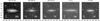 |
Fig. 1. S4G (Sheth et al. 2010) 3.6 micron images of our sample galaxies. Directions on the sky and 2 kpc scale bars are shown on the images. |
To do this, special consideration must be given to the observations, as the eDIG is a low-surface-brightness feature and mapping it requires reaching an Hα surface brightness level lower than ∼10−16 erg s−1 cm−2 arcsec−2 (i.e., it has emission measure below ∼50 cm−6 pc). In addition to good sensitivity, a comprehensive study of eDIG requires good spatial resolution, as well as the coverage of several emission lines. For this reason, integral field unit (IFU) spectroscopy has emerged as an excellent tool in its study. Recent IFU spectroscopy has demonstrated the complex kinematics and emission-line properties inherent to the eDIG with unprecedented detail (Jones et al. 2017; Levy et al. 2019). Unfortunately, current IFU spectrographs have limited fields of view (FoVs), and they are oversubscribed given their multifaceted uses. They also require a substantial amount of observation time to reach the low surface brightness necessary for eDIG observations. Narrowband emission-line imaging provides a faster, albeit less detailed, alternative, with a vast selection of different sized telescopes and instruments with different FoVs available. While it is limited to targeting only one band at a time, this is not an issue for morphological studies, and narrowband imaging is still an indispensable method to complement IFU observations.
To fully describe the eDIG, in addition to understanding its morphology and emission-line properties, one must also understand its kinematics. The kinematics are especially useful in determining the origin of the extraplanar gas, which may be external – accretion from the intergalactic or circumgalactic medium (Oort 1970; Binney 2005; Kaufmann et al. 2006; Sancisi et al. 2008) – or internal – ejected from the galaxy via galactic fountains (Shapiro & Field 1976; Bregman 1980; Fraternali et al. 2002, 2015; Fraternali & Binney 2008). Radial variations in the negative vertical velocity gradient, or lag, of the ionized gas are expected to depend on the origin of the extraplanar gas (Levy et al. 2019). Bizyaev et al. (2017) argued that the correlations they found between the lag and the galactic stellar mass, central velocity dispersion, and axial ratio of the light distribution suggest a possible higher ratio of infalling-to-local gas in massive early-type disk galaxies compared to lower-mass late-type galaxies.
In this work we present the first detailed study of eDIG in a sample of nearby low-mass edge-on galaxies. Our sample is drawn from the sample of Comerón et al. (2019), who serendipitously discovered eDIG in Multi Unit Spectroscopic Explorer (MUSE; Bacon et al. 2010) data of eight edge-on galaxies drawn from the Spitzer Survey of Stellar Structure in Galaxies (S4G; Sheth et al. 2010). To obtain a complete picture of the extended Hα morphology, we acquired deep Hα narrowband imaging of five of those galaxies with the New Technology Telescope (NTT) at La Silla Observatory and the Nordic Optical Telescope (NOT) at the Observatorio del Roque de los Muchachos. Our sample offers a unique combination of depth, spatial resolution, and wavelength coverage for the study of eDIG ionization and formation mechanisms in low-mass galaxies. In our analysis, we use Hα profiles and emission-line diagnostics to investigate the prevalent ionization mechanisms for the extraplanar gas, and ionized gas kinematics to investigate the origin of the gas.
We describe the sample selection, observations, and data reduction in Sect. 2. In Sect. 3 we conduct a photometric analysis of our Hα narrowband imaging, including deriving star formation rates (SFRs), eDIG scale heights (hzeDIG), and Hα radial profiles. We compare these results to a similar analysis of archival Galaxy Evolution Explorer (GALEX) far-ultraviolet (FUV) data in Sect. 4. In Sect. 5 we perform a kinematic analysis of our MUSE data, measuring ionized gas velocity lags and investigating the radial variations in the lag. We investigate the prevalent ionization mechanisms in Sect. 6 with emission-line diagnostics. The individual galaxies are discussed in Sect. 7. In Sect. 8 we discuss our results in the context of the ionization source and origin of the eDIG. The results of this work are summarized in Sect. 9.
2. Observations and data reduction
2.1. The sample
Our sample is derived from that of Comerón et al. (2019), who observed eight edge-on galaxies with MUSE at the Very Large Telescope (VLT) of the European Southern Observatory (ESO), at Paranal Observatory, Chile. The galaxies were selected from the S4G-selected 70 edge-on disk sample of Comerón et al. (2012) chosen to be observable from the Southern Hemisphere and to have an r25 < 60″ (as given in the HyperLEDA1 database; Makarov et al. 2014), so that the region between the center of the target and its edge could be covered in a single MUSE pointing. The quality of the data led to the serendipitous discovery of eDIG in all of the galaxies. In this paper we study the sample of five galaxies for which we were able to obtain deep narrowband imaging in addition to the MUSE data: ESO 157-49, ESO 469-15, ESO 544-27, IC 217, and IC 1553. Fundamental properties of the galaxies can be found in Table 1 and S4G images of the galaxies are shown in Fig. 1. We plan to obtain narrowband imaging for two additional galaxies (PGC 28308 and PGC 30591), which will be included in future work.
Basic properties of our galaxy sample.
2.2. MUSE observations
Our MUSE observations consist of four 2624 s on-target exposures for each galaxy except IC 217, for which three such exposures were taken. The exposures were centered on the same position for each galaxy, with 90° rotations between exposures, totaling nearly three hours of exposure time for the covered areas (except for IC 217, which had two hours and ten minutes).
The data were reduced with the MUSE pipeline (Weilbacher et al. 2012) within the Reflex environment (Freudling et al. 2013) and the combined datacubes were cleaned of sky residuals with the Zurich Atmosphere Purge (ZAP; Soto et al. 2016). The datacubes were tessellated with the Voronoi binning code by Cappellari & Copin (2003) to produce bins with S/N ∼ 50 in Hα. Both stellar and emission-line velocities and velocity dispersions, as well as emission-line intensities were obtained with the Python version of the penalized pixel-fitting code (pPXF; Cappellari & Emsellem 2004). Further details of the MUSE observations, data reduction, Voronoi binning, and the pPXF processing can be found in Comerón et al. (2019).
2.3. Narrowband Hα imaging
MUSE has a FoV of 1′ × 1′. This is small compared to the angular size of the galaxies in our sample and, as such, additional observations were needed to gain critical information about the global spatial distribution of eDIG. We obtained deep narrowband Hα imaging with the ESO Faint Object Spectrograph and Camera (EFOSC2) at the 3.58 m NTT at ESO’s La Silla Observatory in Chile, and the Alhambra Faint Object Spectrograph and Camera (ALFOSC) at the 2.5 m NOT at the Observatorio del Roque de los Muchachos in Spain. EFOSC2 has a FoV of 4 1 × 4
1 × 4 1 and ALFOSC has a FoV of 6
 4 × 6
4 × 6 4, although due to considerable vignetting caused by the filters, the effective FoV of ALFOSC is 4
 45 × 4
 45. These FoVs are large enough to easily cover our galaxies. We used EFOSC2’s standard 2 × 2 binning readout mode, resulting in a pixel scale of 0
 24 px−1. No readout binning was used for ALFOSC, resulting in a pixel scale of 0
 2138 px−1.
We observed ESO 157-49, ESO 469-15, IC 217, and IC 1553 with the NTT over three nights in December 2018. As each galaxy had different observation windows, our total exposure times per galaxy ranged from three to eight hours in our on-band Hα filters (filter number #438 and #761 depending on the galaxy recession velocity), with between 13 to 57 minutes in Gunn r (filter #786) to subtract the stellar continuum. We used filter #761 for ESO 157-49, ESO 469-15 and IC 217, and filter #438 for IC1553, with central wavelengths of 659 nm and 663 nm and full widths at half maximum (FWHMs) of 3 nm and 7 nm, respectively.
We observed ESO 544-27 with the NOT in September 2020. We obtained 12 hours of on-target narrowband Hα exposure (filter #49) and 36 minutes of on-target Gunn r exposure (filter #14). The Hα filter #49 has central wavelength of 661 nm and a FWHM of 5 nm. The exact on-target exposure times for all galaxies are presented in Table 1.
During the NTT data reduction we found that the standard flat-fielding procedure using twilight and dome flats was insufficient to produce uniformly flat backgrounds to our combined images. To avoid these large-scale patterns imposed by the flat-fielding, we constructed night-sky flat-fields from the science images. Due to the galaxies covering a significant portion of the FoV of EFOSC2 and the large amount of masking required because of this, the resulting flats had a relatively poor pixel-to-pixel accuracy. To avoid this issue with the NOT, we also observed a series of off-target blank sky exposures flanking the target field in order to construct the night-sky flats. We observed six hours of night sky in Hα and 18 minutes of night sky in the r band.
We began our data reduction with a standard bias subtraction. We constructed preliminary flat-fields using dome flats taken during the day preceding the observations for the NTT data and exposures of the twilight sky for the NOT data, and applied the flat-field correction to the bias-subtracted science images. Using these preliminary flat-fielded images, we then constructed night-sky flats from both the science and blank sky exposures (for NOT data), following the method described by Mihos et al. (2017). To do this, we first masked astrophysical objects and scattered light artifacts, binned the images, and modeled the sky in each frame using a second-order polynomial fit to all unmasked pixels, using the Astropy2 (Astropy Collaboration 2013, 2018) modeling module’s Levenburg-Marquart least squares fitting routine. We removed the sky gradients from each image by dividing the images with a normalized sky model, then combined these images into a new flat. We then flattened the images using that flat, remade and subtracted the sky models, and masked and binned the images again. We inspected these new images to see if any masks needed adjustment, to catch any diffuse light we missed during our first attempt at masking. If so, we adjusted, or simply did the gradient removal again, and combined the de-skied, masked images into a new flat. We iterated this process until the night-sky flat converged. Next, we flattened the images with this night-sky flat, modeled the skies one more time in the same manner (second-order polynomial), removed those skies from the images, altered the masks to include only leakages, such as scattered light artifacts and satellite trails, and then registered the images in right ascension and declination using Image Reduction and Analysis Facility (IRAF3) software’s WREGISTER task. To account for systematic errors in the frame-to-frame world coordinate system (WCS) registration, we applied offsets using the IMSHIFT task, aligning the images using centroids of a few handpicked stars. This ensures that the on-band and off-band images are perfectly aligned, which is needed for making the continuum-subtracted images. Before the coaddition, we scaled all of the images to a common zero point using the galaxy’s total flux within a large elliptical aperture. Finally, we combined the images to create preliminary coadds.
Possibly due to suboptimal observing conditions – some occurred with the moon above the horizon or during twilight hours, to optimize our time allocation – the night skies in each frame contained complex structure not easily modeled using polynomial fits. To attempt to improve our sky subtraction, we thus employed a novel sky subtraction method using these preliminary coadds (al Sayyad & Lupton, priv. comm.). This involved aligning, flux-scaling, and subtracting the initial coadd from individual science exposures, to remove astrophysical flux and isolate the night sky. Due to the differences in the point spread functions (PSFs) between the initial coadd and the individual exposures, stars, H II regions, and other thin structures like dust lanes are reduced in size but do not perfectly subtract out. Hence, to remove these from our sky maps, we eroded our initial object masks five to ten times using a circular kernel. Additionally, the sky maps generated by coadd-subtraction have extremely high pixel-to-pixel noise, and hence we binned the masked maps with bin sizes on the order of the target galaxy width, interpolated flux across any remaining masked pixels, and applied a Gaussian smoothing using a kernel with a FWHM of half the bin size in px. This results in a lower resolution but far less noisy map of the night sky in each frame, which we then subtracted as the individual frame skies. The resulting image backgrounds are significantly flatter than those produced using the polynomial fit skies. A new flat was constructed from the images again using the new sky models and divided out from the science images. This was again iterated until the new flat converges, and we created a final generation coadd using this final flat-field and these coadd-subtraction sky models. Because this sky subtraction method is novel, we will explore it in greater detail in a separate paper, including demonstrations of low-surface-brightness flux preservation using model galaxy injections. Preliminary tests show that it preserver flux at all surface brightnesses to within ∼5%.
To construct the continuum-subtracted Hα images, the r-band image must be scaled to be proportional to the stellar continuum emission in the Hα filter image. We estimated this scale factor using two methods. First, we plotted the intensity of each pixel in the Hα image against its intensity in the r-band. Pixels with no line-emission have Hα flux that is linearly proportional to the r-band flux and appear as straight line in the plot. Pixels with Hα emission have an excess flux over the stellar continuum, and so appear systematically above this line. The slope of the line gives the scale factor to scale the r image to be subtracted from the Hα image (Knapen 2005; Knapen et al. 2006). Second, we compared the luminosities of the foreground stars in both filters and, under the assumption that those stars have no Hα emission or absorption, took that as a secondary estimate of the scale factor for the r image. These two methods give a range of values for the scale factor, from which we chose the final scale factor by eye so that over-subtraction and residual foreground starlight are minimized.
We flux-calibrated the continuum-subtracted Hα images by using the MUSE data. To do this we constructed mock continuum-subtracted narrowband Hα images from the MUSE cubes by stacking a 60 Å band covering the Hα and [N II] lines and subtracting from it a nearby 60 Å band covering no emission lines. We then calibrated the flux so that the counts in several ∼1″–4″ in radius circular apertures centered on H II regions along the disk in the continuum-subtracted Hα images are equal to those in the MUSE mocks. Both our MUSE and our narrowband observations reach an unbinned 1σ background sensitivity of ∼10−17 erg s−1 cm−2 arcsec−2 in Hα.
2.4. Archival GALEX data
To gain information about the age of the ionizing stellar population as well as the distribution of O and B stars, we retrieved archival GALEX FUV imaging from the Mikulski Archive for Space Telescopes (MAST). The GALEX FUV channel covers wavelengths from 1350 to 1750 Å, and the detector has a pixel scale of 1 5/px and an effective angular resolution of 6″. We use observations from the GALEX All-Sky Imaging Survey, Medium Imaging Survey, and the AKARI Deep Field South guest investigator program (Morrissey et al. 2007; Bianchi 2009). The total exposure times per galaxy vary greatly due to the different depths of the used surveys, ranging from 186 to 1839 s. The exact exposure times are presented in Table 1. The GALEX data described here may be obtained from the MAST archive4.
3. Hα photometry
3.1. Hα luminosity and star formation rates
To investigate the connection between the eDIG ionization and SF, we must first obtain the SFR in our sample galaxies. To do this, we measured the integrated Hα luminosity and the SFR of our galaxies from our narrowband imaging data. We identified sources that appear in the r-band images, but not in the continuum-subtracted Hα images; and sources that appear in the continuum-subtracted Hα images, but show spectra inconsistent with Hα emission of appropriate redshift in the MUSE cubes; as background or foreground sources and masked them out from the continuum-subtracted Hα images. We also masked everything beyond where the galaxies blend into the background in the r band images (pixel signal-to-noise drops down to the background value). We then measured the total Hα flux from the masked images.
To correct for dust extinction, we measured the Balmer decrement using the integrated Hα and Hβ emission from the MUSE cubes and calculated the Hα extinction adopting a Calzetti extinction law (Calzetti et al. 2000) with RV = 4.5 (Fischera & Dopita 2005). The MUSE pointings cover each galaxy only partially, the pointings being centered on one side of the galaxy if the whole disk does not fit into a single MUSE pointing. While this does increase the uncertainty of our extinction estimates, it does not do so significantly, if we believe the reasonable assumption that the dust distribution and extinction has some degree of azimuthal symmetry. We calculated the extinction-corrected Hα luminosity using distances from Tully et al. (2008, 2016). The luminosities are presented in Table 2.
Photometry results.
We calculated the SFR from the extinction-corrected Hα luminosities using the Hao et al. (2011) and the Murphy et al. (2011) calibrations. We find SFR values ranging from 0.13 to 0.96 M⊙ yr−1. We also calculated the specific SFR (sSFR = SFR ) using 3.6 μm stellar masses from Muñoz-Mateos et al. (2015). The SFR and sSFR are presented in Table 2 and the SFR–M* relation for our sample is shown in Fig. 2. Of our galaxies, only IC 1553 is firmly in the star-forming main sequence (Noeske et al. 2007). ESO 157-49, ESO 469-15, and IC 217 are also marginally star-forming when star-forming galaxies are defined as those with sSFR > 10−10.6 yr−1 (Hsieh et al. 2017), while ESO 544-27 falls into the green valley.
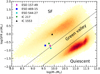 |
Fig. 2. Stellar mass against SFR relation for our sample. The heatmap represents Sloan Digital Sky Survey (SDSS) galaxies with M* from Kauffmann et al. (2003b) and Salim et al. (2007) and the SFR from Brinchmann et al. (2004). The dashed lines correspond to constant sSFRs of 10−10.6 and 10−11.4 yr−1. These lines separate star-forming galaxies, the green valley, and quiescent galaxies (Hsieh et al. 2017). |
3.2. Vertical profiles and scale heights
To characterize eDIG and its spatial distribution, we obtained vertical Hα profiles from the narrowband data. We estimated the alignment of the disk planes using the position angles from Salo et al. (2015). We also masked ESO 469-15’s extraplanar H II regions so they do not influence the eDIG measurements.
To obtain the vertical profiles of the ionized gas, we averaged the Hα intensity at each height over the plane of the galaxy in one-pixel-wide bins. We radially restricted the measurement to areas with clear visually identifiable midplane H II regions. We then modeled the vertical profile with two exponential disks. We also attempted to fit the vertical profile at different radii in one scale length bins but find that our data are not sensitive enough for well-constrained two-component fits when not integrating over the whole disk.
The shape of the surface brightness profiles is also affected by the PSF of the data. To obtain the PSF we adopted a method similar to Infante-Sainz et al. (2020), using stars with different brightnesses to measure different parts of the PSF. For the NTT data, we modeled the PSF by combining an averaged core PSF of several bright stars in the data with mid-range PSF obtained from the brightest star in the data. We do not have bright enough stars in our data to measure the arcminute-scale extended wings of the PSF, but because it is primarily these faint wings that bias the light profiles of galaxies at low surface brightness (Rudick et al. 2009; Sandin 2014, 2015), we instead extrapolated the measured PSF down below the image noise limits using mock wings following a r−2 power-law. A power-law r−2 was chosen as it is a common slope in the PSF wings of ground based observations (King 1971; Slater et al. 2009; Sandin 2014). We experimented with other values for the wing slopes, ranging from r−1.5 to r−2.5, and found the effect to be negligible to our results. The averaged core PSF extended out to 3 6, the middle section from the single bright star to 16
 9, and the power law wings out to 150″.
We attempted to model the NOT PSF in a similar manner, but our observations with this telescope lacked sufficiently bright stars to create this three-stage PSF. Instead we made the PSF from two stages of the averaged core within 5 3 and a mock power law wings beyond that. The wings are clearly steeper for the NOT data so we used power-law of r−2.5. Radial profiles of the PSFs are shown in Fig. 3.
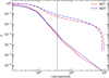 |
Fig. 3. PSF radial profiles measured and extrapolated from our NTT (red lines) and NOT (blue lines) data. The dashed lines show the extrapolated power-law wings. The dot-dashed lines indicate the fractional cumulative flux outside a given distance from the center. The black vertical dashed line corresponds to the separation between the averaged core PSF and the bright star middle section at 3 |

We created 2D images of our double-exponential model, then convolved them with our 2D PSFs. We then extracted the vertical profiles from these convolved model images and fit these to the measured vertical profiles, leaving the scale heights and central fluxes of the two components, as well as the midplane position (z = 0) as free parameters. We interpret the scale height of the thinner component as the vertical extent of the in-plane H II regions (hzH II in Table 2). Then we fit the profile again but masked the previously obtained H II region dominated thin disk region |z| < hzH II and constrain the midplane to the same z as obtained from the first fit. For the second fit we adopt the interpretation of Miller & Veilleux (2003a), where the thinner component of the remaining Hα emission is the brighter quiescent phase of DIG and the thicker component is the fainter disturbed extraplanar phase of DIG, or eDIG. We used Poisson weighting in the fits. The scale heights obtained from these fits are presented in Table 2 (hzDIG and hzeDIG) and the fits and profiles themselves are shown in Fig. 4. For the quiescent component we obtain scale height values ranging from 0.12 to 0.24 kpc and for the disturbed eDIG from 0.59 to 1.39 kpc.
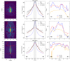 |
Fig. 4. Masked narrowband Hα images (left) and vertical (center) and radial (right) Hα profiles for our sample. Black dots in the center column show measured fluxes, and the black curves show our two-component exponential fits. The dashed blue curve in the center column is the thinner component of the fit, representing the quiescent phase of the DIG. The dashed red curve in the center column is the thicker component of the fit, representing the disturbed eDIG. The fit scale heights are shown for both components in the legends of the center column. The vertical dashed black lines in the center column are the inner limits of lenient (inner) and stringent (outer) eDIG definitions (see text). These are also shown in the Hα images of the left column via the vertical solid red lines. The horizontal solid red lines in the left column show the radial extent of the thin disk and eDIG definitions. In the right column the solid blue lines represents the thin disk radial Hα profiles, the solid red lines represents the eDIG radial Hα profiles using the lenient eDIG definition (eDIG1), and the solid orange lines represent the eDIG radial Hα profiles using the stringent eDIG definition (eDIG2). The thin disk and lenient eDIG radial profiles are normalized to unity flux, and the stringent eDIG radial profiles are normalized to the flux of the lenient eDIG flux to highlight the similarities between the profiles. The disk–eDIG Pearson r values are shown in the legends of the right column. Directions on the sky are indicated in the images and the plots. |
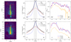 |
Fig. 4. continued. |
Most previous eDIG scale height measurements in literature have relied on single-exponential fits due to insufficient sensitivity. To better compare our results to these previous works, we obtained single-exponential Hα scale heights from our data in the same manner we obtained the double-exponential scale heights, except we modeled the vertical profiles with a single-exponential disk and a constant background instead of two exponential disks. The single-exponential fits give scale heights ranging from 0.14 to 0.35 kpc (hz1 in Table 2). Our scale height measurements were performed on sky-corrected images where the background should be near zero, but the single-exponential fits require positive backgrounds with surface brightness on the order of our sensitivity limit. This may be caused by the emission from the disturbed eDIG affecting the backgrounds, suggesting that a single-exponential fits are insufficient in modeling the Hα vertical profiles of our sample galaxies. We also experimented with the van der Kruit (1988) three-parameter vertical density profile5, but found that the fits tended toward the limiting case of an exponential disk (n = ∞). Figure 5 illustrates how single-component fits fail to model simultaneously both the steep quiescent DIG near the midplane and the extended disturbed eDIG at large heights.
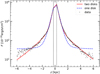 |
Fig. 5. Comparison of vertical Hα profile fits of IC 1553 using our double-exponential model (solid red line) and single-exponential model with a constant background (dashed blue line). Black dots show the measured fluxes, and the black vertical dashed lines show the extent of the thin disk. |
To test the goodness of fit of our models we calculated the χ2 and Bayesian information criterion (BIC; see Schwarz 1978) values for our double-exponential and single-exponential fits. The χ2 is defined as
![Mathematical equation: $$ \begin{aligned} \chi ^2 = \sum _z^{n_z} \frac{[I_{\rm obs}(z) - I_{\rm model}(z)]^2}{\sigma (z)^2}, \end{aligned} $$](/articles/aa/full_html/2022/03/aa42440-21/aa42440-21-eq15.gif) (1)
(1)
where Iobs is the observed intensity of the profile, Imodel is the intensity of the fitted model, σ is the Poisson uncertainty of the measured profile calculated using background standard deviation and the effective gain of the combined image, and the sum is calculated over the vertical profile. If the data are well described by the model, χ2 will be approximately equal to the number of degrees of freedom ν = nz − k, where nz is the number of vertical bins in the profiles and k is the number of free parameters in the models. The latter is four for our double-exponential model (central intensities and scale heights of the two disk) and three for our single-exponential model (central intensity and scale height of the disk and the intensity of the constant background). The BIC, formulated (according to Kass & Raftery 1995) as
 (2)
(2)
is based on the χ2, but adds a second term that penalizes model complexity. This way, BIC is a good statistic when comparing models with different numbers of components, giving larger (worse) values to overfitted models. The normalized χ2 values (χ2/ν) and BIC values for our double-exponential and single-exponential fits are given in Table 2. The double-exponential fits have smaller (better) χ2/ν and BIC values than the single-exponential fits for all our galaxies, indicating that the double-exponential fits represent our data more accurately. However, we find χ2/ν values much greater than one for even our double-exponential fits, suggesting that neither double-exponential nor single-exponential disks describe the eDIG very well. This is not surprising considering the filamentary and asymmetric eDIG morphology present in our sample galaxies. While scale heights derived from exponential disk models are a useful tool to measure the vertical extent of eDIG, it is clear that simple exponential disks cannot describe eDIG fully.
Miller & Veilleux (2003a) use double-exponential fits to the Hα vertical profile and find a median scale height of 2.3 ± 4.3 kpc and a range of values from 0.4 to 17.9 kpc for the disturbed eDIG component over their sample of 16 galaxies. Figure 6 shows the scaling relation between M* and hzeDIG for our sample and for those galaxies of Miller & Veilleux (2003a) for which stellar masses were derived by Muñoz-Mateos et al. (2015). Levy et al. (2019) find a median scale height of  kpc with single-exponential fit over their sample of 25 edge-on galaxies from the Calar Alto Legacy Integral Field Area Survey (CALIFA). They measure scale heights ranging from 0.3 to 2.9 kpc in galaxies with stellar masses ranging from 109 to 1011 M⊙. Furthermore, Levy et al. (2019) compiled an extensive list of eDIG scale heights from various sources (Rand 1997; Wang et al. 1997; Hoopes et al. 1999; Collins et al. 2000; Collins & Rand 2001; Miller & Veilleux 2003a; Rosado et al. 2013; Bizyaev et al. 2017) and found a median eDIG scale height of 1.0 ± 2.2 kpc. While there is considerable scatter from galaxy to galaxy in the eDIG measurements in literature, our values – using both double-exponential and single-exponential fits – are still well within the large range of previous scale height measurements.
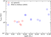 |
Fig. 6. Stellar mass against eDIG scale height for our sample galaxies (red diamonds) and for a subset of Miller & Veilleux (2003a) sample galaxies for which stellar masses were derived by Muñoz-Mateos et al. (2015) (blue squares). |
3.3. Radial profiles
To complete our characterization of the eDIG with the spatial distribution along the radial axis, we measured the radial profiles of the ionized gas both in the thin disk and in the extraplanar regions. For the thin disk we averaged the Hα intensity in 4 pixel wide radial bins over the vertical extent of the H II-region-dominated thin disk, using the same thin disk region described in Sect. 3.2 (|z| < hzH II). The width of the radial bins (4 pixels) was chosen to be on the order of the PSF FWHM, in order to minimize PSF effects along the radial axis. For the extraplanar gas we used two different eDIG area definitions to investigate the effects of vertical PSF contamination from the bright disk H II regions. For a lenient eDIG definition (eDIG1) we averaged the radial Hα intensity over the heights above and below the thin disk up to the background mask (|z| > hzH II). For a stringent eDIG definition (eDIG2) we averaged the radial Hα intensity from |z| > 3hzH II to the background mask, leaving a 2hzH II buffer region between the thin disk and the stringent eDIG that is not used in either radial profile. The radial profiles are shown in Fig. 4.
We then calculated the Pearson correlation coefficients between the thin disk radial profile and the two eDIG radial profiles with the intention of quantifying the spatial correlation between the disk H II regions and eDIG. A similar approach using a single eDIG definition was done by Miller & Veilleux (2003a). The Pearson correlation coefficients between the H II-region-dominated disk and the lenient and stringent eDIG (r values) are given in Table 3. A correlation coefficient of 1 (−1) would signify a perfect (anti)correlation, while 0 would mean no correlation. Using the lenient eDIG definition all galaxies show some degree of correlation with the lowest r value being 0.55 and the highest 0.94. Using the stringent eDIG definition does not greatly affect the correlation in the galaxies with the strongest correlations (ESO 469-15, IC 217, and IC 1553), but it does significantly weaken the correlation in the galaxies with the weakest correlations (ESO 157-49 and ESO 544-27), with a minimum of 0.15 in the case of ESO 544-27. This shows that while the correlation between the lenient eDIG and the thin disk may be strongly influenced by PSF in ESO 157-49 and ESO 544-27, this is clearly not the case for ESO 469-15, IC 217, and IC 1553. It should be noted that regardless of PSF contamination, the correlation coefficients between the eDIG and the thin disk radial profiles depend on the height at which the eDIG radial profile is measured, as illustrated by Fig. 7. Also given in Table 3 are the correlation p-values, which roughly indicate the probability of an uncorrelated system producing data sets with at least as high Pearson r as the data set in question. The highest p-value for our correlations is ∼0.28 for the stringent eDIG of ESO 544-27, indicating a 28% probability of the radial profiles being uncorrelated, while the other p-values indicate probabilities of less than 5%. There is clearly a significant positive correlation between the disk and eDIG Hα emission, suggesting that leaky H II regions are indeed an important source of ionization for the eDIG.
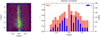 |
Fig. 7. Disk–eDIG radial profile Pearson correlation at different heights for IC 217. Left panel: Hα image of the galaxy. Right panel: correlation coefficient (r; red bars) and the p-value (p; blue bars) at different heights (z). The red rectangles in the left panel correspond to the bins from which the eDIG radial profiles at different heights were measured. |
Radial profile correlations.
Dust obscuration is much more impactful to the disk radial Hα profile compared to the eDIG profiles. To test whether dust obscuration is weakening our correlations, we derived raw and extinction corrected (using the Balmer decrement) Hα maps from our MUSE cubes, and performed the radial profile correlation analysis described above on them. Due to the MUSE FoV being smaller than the radial extent of some of our sample galaxies, the MUSE cube derived profiles are not comparable to our narrowband imaging profiles. However, differences between the MUSE-derived extinction-corrected and raw Hα maps should demonstrate the effects of dust obscuration on our analysis. We do not find significantly stronger correlations on the extinction corrected Hα maps compared to the raw Hα maps for any of our galaxies. On the contrary, most correlations are slightly weakened on the extinction corrected images. This is most likely caused by the increased noise on the extinction corrected Hα maps. Dust obscuration does not seem to have significant effect on our radial profile correlation analysis.
3.4. Trends with SFR
Now that we have both obtained the SFR and characterized the eDIG spatial distribution in our sample, we can investigate their connection. Correlations between the eDIG properties and the SFR are expected if the eDIG is a result of star-forming activity. If leaky H II regions in the thin disk drive the eDIG ionization, one would expect a positive correlation between the sSFR and the eDIG scale height. If other mechanisms also play part in the ionization of eDIG, one might expect the disk and the eDIG Hα emission to be more strongly spatially correlated in galaxies with higher sSFR.
We compare the measured eDIG scale heights and disk–eDIG r values to sSFR in Figs. 8 and 9. There appears to be a clear positive correlation between the sSFR and the eDIG scale height, supporting a link between the disk SF and the eDIG ionization. There is also a positive correlation between sSFR and disk–eDIG r values. For the disk–eDIG r values, using the stringent eDIG area definition less affected by the PSF contamination results in an even stronger correlation with the sSFR. The positive correlation between sSFR and disk–eDIG r values suggests that in galaxies with less SF, other mechanisms may contribute to the eDIG ionization significantly, and thus weaken the correlation between disk and eDIG Hα emission. Given our small sample size (N = 5), we admit that these correlations may be spurious. However, we find them worth noting since in Sect. 6 we show stronger evidence supporting a scheme of eDIG ionization with OB stars as the primary source along with other contributing ionization mechanisms.
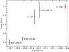 |
Fig. 8. Specific SFR against eDIG scale height for our sample. One-standard-deviation error bars of the hzeDIG fit are shown. |
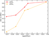 |
Fig. 9. Specific SFR against disk–eDIG radial profile Pearson correlation for our sample. The solid red line is computed using our lenient eDIG definition (eDIG1) and the dashed orange line using our stringent eDIG definition (eDIG2). |
We also investigated correlations between the eDIG properties and other global galaxy properties, such as D25 (the diameter of the B-band isophote corresponding to 25 mag arcsec−2; de Vaucouleurs et al. 1991), the scale length (hR), and the heights of the stellar disks (hzt and hzT), M*, and the color excess (the difference between an object’s observed color index and its intrinsic color index), but find no clear correlations. However, this does not imply anything definitive about the underlying population of nearby low-mass disk galaxies, as our M* range is very limited and we lack the necessary statistics.
4. Comparison with GALEX data
Ionizing stellar emission comes in the form of LyC photons that have wavelengths below 912 Å. While GALEX FUV does not cover LyC, it is nonetheless a good proxy to map the emission of bright, ionizing stars. FUV traces O and B stars down to 3 M⊙ (Kennicutt & Evans 2012). By comparing the FUV and the Hα emission we can infer information about the age of the ionizing stellar population, as hotter early type stars emit more in LyC and as such will cause more gas ionization and more Hα emission (Hoopes & Walterbos 2000; Hoopes et al. 2001; Seon et al. 2011). Hα emission traces SF that has occurred within 20 Myr while FUV traces SF that has occurred within 100 Myr (Kennicutt 1998).
We measured the FUV flux from the GALEX data using the same masks as we did with the Hα images. To correct for dust extinction, we again used the Balmer decrement from the MUSE cubes and calculated the FUV extinction adopting a Calzetti extinction law (Calzetti et al. 2000) with RV = 4.5 (Fischera & Dopita 2005). To gain a measure of the age of the ionizing stellar population, we calculated the Hα/FUV intensity ratios from extinction-corrected Hα and FUV luminosities. The Hα/FUV intensity ratio correlates well with the Hα derived sSFR (Fig. 10), as one would expect since galaxies with ongoing starbursts naturally have younger stellar populations.
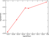 |
Fig. 10. Specific SFR against Hα/FUV intensity ratio for our sample. |
To assess the comparability between the Hα and the FUV scale heights, we extracted the vertical FUV profile using the same masking and spatial limits that we used with the vertical Hα profiles in Sect. 3.2. The GALEX data are not sensitive enough for well-constrained double-exponential fits, so we modeled the vertical FUV profile as a single component exponential with a constant background, convolved the model with PSF retrieved from the GALEX online technical documentation6, and fit it to the profile. We obtain FUV scale heights (hzFUV) ranging from 0.26 to 0.98 kpc. The FUV scale heights and extinction-corrected luminosities as well as Hα/FUV intensity ratios are presented in Table 4.
FUV properties.
Jo et al. (2018) find a strong correlation between the Hα and the FUV scale heights in their sample of 38 nearby edge-on galaxies using single-exponential fits for both FUV and Hα. In the galaxies in which they detect extraplanar FUV emission (hzFUV > 0.4 kpc) they find that the scale height in Hα is on average 0.74 times the scale height in FUV. In contrast, we find that hzeDIG is larger than hzFUV for all but one of our galaxies (ESO 544-27). There is also no evidence of any correlation between hzeDIG and hzFUV in our sample. However, as can be seen from Fig. 11, our single-exponential fit Hα scale heights do follow a similar relation with FUV scale heights as the Jo et al. (2018) sample. This seems to suggest that the correlation Jo et al. (2018) find between the Hα and the FUV scale heights may break down at lower surface brightness levels and more thorough two-disk modeling of the eDIG. We however note that our Hα imaging is deeper and has better resolution than the GALEX FUV imaging used in Jo et al. (2018) as well as in this work. It is possible that with more sensitive FUV data, a two-component morphology might emerge in FUV as well, which might again give rise to a correlation between FUV and eDIG scale heights.
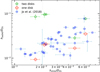 |
Fig. 11. FUV scale height against eDIG scale height for our sample using double-exponential fits (green pentagons) and Jo et al. (2018) sample (blue squares). The scale heights are normalized by the D25 of the host galaxies. One-standard-deviation error bars for the scale height fits are shown in lighter colors. It should be noted that Jo et al. (2018) use single-exponential fits while ours are two-component fits. For comparison, we also show the scale height ratios for our sample using similar single-exponential fits as adopted by Jo et al. (red diamonds). |
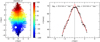 |
Fig. 12. Velocity lag in ESO 544-27. Left panel: velocity map. Right panel: vertical velocity profile. The velocity profile has been obtained by averaging the absolute velocity at each height. The black dashed line in both the map and the profile indicates the midplane. The black dots show the measured velocities, and the red lines show the fits to the velocity profile on both sides of the midplane. The absolute values of the slopes of the lines, or the lags above and below the midplane, are given in the right panel. |
5. Ionized gas kinematics
5.1. Vertical gradients in the ionized gas rotation velocity
To construct a full picture of the eDIG, we must understand its kinematics in addition to its photometry and morphology. To gain a general sense of the eDIG kinematics in our sample, we constructed position-velocity (PV) diagrams of the ionized gas from the Voronoi binned velocity maps by calculating the vertical and radial distance between the center of the galaxy and the median height (z) and radius (r) pixel coordinates of each bin. The PV diagrams show evidence of a decrease in the line-of-sight velocity of the ionized gas with increasing distance from the midplane. This is a common property of ionized gas (Miller & Veilleux 2003b; Bizyaev et al. 2017; Levy et al. 2019).
Such a negative vertical gradient is often called lag, and can be quantified as −ΔV/Δ|z| in units of km s−1 kpc−1. We measured the radially averaged lag from our velocity maps by averaging the absolute velocity in one pixel wide bins at each height above and below the midplane over the disk radial extent to obtain a vertical velocity profile, and then fit a line to this profile above and below the midplane. The slopes of the lines give the lag above and below the midplane. Figure 12 shows the velocity map and vertical velocity profile of ESO 544-27 as an example. The lag (average of the values above and below midplane) is given for each galaxy in Table 5. We obtain lag values ranging from 9.76 to 27.4 km s−1 kpc−1. The velocity maps and PV diagrams are presented in Fig. 13.
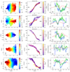 |
Fig. 13. Velocity maps (left), PV diagrams (middle), and lag profiles (right) for the galaxies of our sample. The size of the points in the middle column corresponds to the size of the Voronoi bins they represent. The red curves in the right column show the lag profile of our N-body simulation, scaled to the maximum rotation velocity and to the scale length of the galaxy; this profile corresponds to circular orbits in a steady axisymmetric potential. The solid blue lines and the dashed green lines in the right column show the measured lags above and below the midplane of the galaxy, with the direction indicated in the legend. The uncertainties of the two lag fits are shown in lighter colors. Directions on the sky are indicated in the plots. |
Ionized gas kinematics.
Levy et al. (2019) find measurable lags in 60% of the galaxies in their sample, with values ranging from −10 to 70 km s−1 kpc−1. The median for their complete sample is  km s−1 kpc−1, or
  km s−1 kpc−1 if galaxies with no measurable lag and negative lag (velocity increases with increasing z) are excluded. They also compiled lag measurements from literature (Miller & Veilleux 2003b; Heald et al. 2006b,a, 2007; Bizyaev et al. 2017) and find a median lag of
  km s−1 kpc−1. Our lag measurements fall into same range as the Levy et al. (2019) and other literature values, indicating that the gas kinematics of our sample galaxies are typical of edge-on galaxies.
5.2. Radial gradients in the velocity lag
Different formation scenarios for extraplanar gas can give rise to different radial gradients (∂lag/∂r) in the lag (Levy et al. 2019). For an internal origin of the gas one might expect a decrease in the lag with radius, as for gas ejected to a given height, a centrally concentrated potential will slow down gas more if said gas is ejected from a small radius than if said gas is ejected from a large radius (Zschaechner et al. 2015). With accretion that is parallel or inclined to the angular momentum axis, no radial variation in the lag is expected (Kaufmann et al. 2006; Binney 2005). If accretion instead happens from cold gas at the outskirts of the galaxy, the gas will spiral in progressively (Combes 2014). This could result in larger lags at larger radii if the rotation velocity of the accreted gas increases as it spirals in.
However, regardless of the origin of the gas, the velocity lag and its radial gradient are affected by the shape of the galaxy potential. Therefore, even in the case of gas rotating in circular orbits in a steady axisymmetric galaxy, nonzero velocity lags and radial lag profiles are present.
Levy et al. (2019) study the radial variations in the lag with the aim of determining the origin of the extraplanar gas. They find that galaxy potential alone is enough to explain the lag radial variations in their sample. They compared ∂lag/∂r measured from their sample of 25 edge-on CALIFA galaxies to ∂lag/∂r calculated from a Miyamoto-Nagai model potential and find the measured values broadly consistent with the analytic expectation for gas in circular orbits. The model galaxy potential induces lag radial gradients comparable to those they measured. They conclude that the galaxy potential is the primary contributor to ∂lag/∂r within their galaxy sample, and the effect of a gas’s origins is impossible to discriminate at their resolution and uncertainties.
We attempt a similar analysis for our galaxy sample. Our data may be more amenable to such analysis because of our greater depth and resolution. MUSE has a 1′ × 1′ FoV sampled at 0 2 × 0
2 × 0 2, compared to the 331 science fibers covering a FoV of 74″ × 64″ of the Potsdam Multi Aperture Spectrograph (PMAS; Roth et al. 2005) in the PMAS fiber package (PPak; Verheijen et al. 2004; Kelz et al. 2006) mode used by CALIFA. Additionally, our MUSE data consist of more than two hours of exposure for each galaxy with the 8.2 m VLT, compared to the 45 minutes of exposure per galaxy with the 3.5 m telescope of the Calar Alto observatory in the CALIFA V500 setup (Sánchez et al. 2012). This allows us to more accurately measure ∂lag/∂r and to plot lag as a function of r for individual galaxies.
To take line-of-sight integration effects properly into account, we used an N-body simulation model to estimate the typical ∂lag/∂r caused by the potential. The N-body model that we use is the same axisymmetric equilibrium model that is used in Comerón et al. (2019) to test for retrograde motion in thin+thick disk galaxies. Its parameters were chosen to represent low-mass galaxies with no significant bulge component – similar to our sample galaxies. When applied to our observed galaxies, the N-body data were scaled to have a similar radial stellar disk scale length and maximum rotation velocity as the observed galaxy. More details of the model and how it is constructed are available in Comerón et al. (2019) and Salo & Laurikainen (2017).
To obtain the radial profiles of the velocity lag in our sample galaxies, we measured the lag as above, except we did not average over the whole disk and instead measured the lag separately at each radius in 1″ bins. From this we obtained the radial lag profiles above and below the midplane separately. Similarly, we obtained the potential induced radial lag profile of our N-body simulation. Compared to the Miyamoto-Nagai model derived lag curve of Levy et al. (2019), our model curve is qualitatively quite similar. The measured and model lag profiles are compared in Fig. 13. We also calculated linear fit ∂lag/∂r for our galaxies, which can be found in Table 5.
All of the measured lag profiles are highly disturbed compared to the N-body model lag profile. For IC 217 and the southwestern side of ESO 544-27 however, while the measured profiles are disturbed, they more or less follow the model profile and do not deviate from it systematically. ESO 469-15 on the contrary, has significantly stronger lag at all radii compared to the simulation model. This results also in a steeper radial lag gradient in the central parts of the galaxy. This gradient is likely not related to radial inflow but rather to the extraplanar H II regions of ESO 469-15, which seem to have greater lag than the more diffuse extraplanar gas of the other galaxies. ESO 157-49, IC 1553, and to a lesser extent the northeastern side of ESO 544-27 also have systematic differences to the model. They have highly asymmetric lag profiles, with only one side broadly consistent with the model profile. The opposite sides, by contrast show nearly inverse behavior to that of the model, with consistently increasing lag with radius and negative lag (gas rotation velocity increases with height) near the center of the galaxy. The positive radial gradient of the lag could indicate accretion by radial inflow, although that would not explain the negative lag near the center of the galaxy.
Asymmetries in galaxies are often associated with galaxy interactions or accretion. In our sample only ESO 157-49 has nearby companions; the other galaxies have no neighbors with measured redshifts within 1° and 1000 km s−1. ESO 157-49 has three smaller dwarf neighbors with similar recession velocities, the closest of them being ESO 157-48 located 14.2 kpc projected distance southwest of the galaxy, while the others have projected distances greater than 100 kpc. The direction to ESO 157-48 is parallel to the plane of ESO 157-49, and ESO 157-49 has a positive radial lag gradient on the side nearest to ESO 157-48. The asymmetry and the positive lag gradient of ESO 157-49 could be thus related to interactions with this dwarf companion. As IC 1553 has no known nearby companions, accretion from a diffuse source seems like a more plausible explanation for its distorted eDIG morphology and kinematics.
6. Emission-line diagnostics
6.1. Hα equivalent width in the eDIG
Above we showed that SF in the thin disk correlates well with eDIG ionization. To confirm the significance of OB stars to eDIG ionization and to investigate the contribution of evolved stars and shocks, we examined the gas recombination emission-line spectrum. The equivalent width (EW) of the Hα emission line can be used to identify ionization by hot low-mass evolved stars (HOLMES; Flores-Fajardo et al. 2011). HOLMES are post asymptotic giant branch stars and white dwarfs that are plentiful in the thick disks and lower halos of galaxies. Their greater scale height compared to OB stars and their significant contribution to the UV radiation of galaxies (Hills 1972; Rose & Wentzel 1973; Terzian 1974; Lyon 1975), makes them a promising potential source of eDIG ionization.
The EW of Hα is defined as EW(Hα) = LHα/CHα, where CHα is the continuum luminosity around Hα. As the continuum luminosity is determined mostly by the emission of evolved stars, EW(Hα) has a strong anticorrelation with the age of the ionizing population (Cid Fernandes et al. 2011; Lacerda et al. 2018). The EW(Hα) distribution among and within galaxies is strongly bimodal (Bamford et al. 2008; Cid Fernandes et al. 2011; Belfiore et al. 2016; Lacerda et al. 2018). Lacerda et al. (2018) interpret the peak at ∼3 Å to be caused by a population of HOLMES ionized gas and the peak at ∼14 Å to be caused by a population of OB star ionized gas. From this they derive a division of EW(Hα) < 3 Å as ionization dominated by HOLMES, EW(Hα) > 14 Å as ionization dominated by OB stars, and 3 Å < EW(Hα) < 14 Å as a mixed regime where both HOLMES and SF complexes contribute to the ionization. López-Cobá et al. (2019) also use this division, while Levy et al. (2019) use a simplified scheme where EW(Hα) = 6 is the division between gas ionized by star-forming H II regions and gas ionized by other means such as shocks and HOLMES.
We obtained EW(Hα) maps by dividing the fitted Hα flux by the fitted stellar flux at the wavelength of Hα in each Voronoi bin. We find no Voronoi bins with EW(Hα) < 3 Å in any of our galaxies and only few isolated bins with EW(Hα) < 6 Å. We conclude that HOLMES are not the primary ionization source of eDIG in any of our galaxies. However, we find many extraplanar Voronoi bins that have EW(Hα) < 14 Å, meaning HOLMES could be a significant secondary ionization source in these regions. The distribution of this secondary HOLMES ionization differs significantly between the galaxies, ESO 544-27 having EW(Hα) < 14 Å nearly everywhere outside the disk, while IC 1553 has EW(Hα) < 14 Å only in few extraplanar regions on the northern side of the disk. The EW(Hα) maps are presented in Fig. 14.
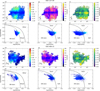 |
Fig. 14. Emission-line properties in our sample galaxies. (a) η-parameter maps (Erroz-Ferrer et al. 2019). (b) Velocity dispersion maps. (c) Logarithmic EW(Hα) maps. (d), (e), (f) VO diagrams. The solid line in the VO diagrams is the Kewley et al. (2001) extreme starburst line, the dashed line is the Kauffmann et al. (2003a) empirical starburst line, and the dash-dot line is the Kewley et al. (2006) Seyfert-LINER demarcation line. The colors in the VO diagrams correspond to the colors in the η-parameter maps. The lower limit of the OB-star-dominated ionization (EW(Hα) = 14 Å) is contoured in black on the EW(Hα) maps. |
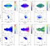 |
Fig. 14. continued. |
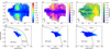 |
Fig. 14. continued. |
6.2. Emission-line ratios in the eDIG
To gain more information about the ionizing spectrum, we constructed emission-line ratio maps from the Voronoi binned MUSE data. We confirm that [N II]/Hα, [S II]/Hα and [O I]/Hα line ratios are generally enhanced in the eDIG compared to the in-plane H II regions, with some differences between galaxies. We also find [O III]/Hβ to be enhanced to some degree in the eDIG of all galaxies except IC 217.
As a single line ratio may depend on many factors such as gas density or temperature, diagnostic diagrams using two different line ratios are better at discriminating different ionizing spectra and their sources. We used the Veilleux-Osterbrock (VO; Veilleux & Osterbrock 1987) suite of diagnostic diagrams, EW(Hα) maps, and ionized gas velocity dispersion (σ) maps to identify shock ionization in our sample galaxies. Firs, we used the classic [N II]/Hα versus [O III]/Hβ Baldwin-Phillips-Terlevich (BPT; Baldwin et al. 1981) diagram, in conjunction with the Kewley et al. (2001) extreme starburst line and the Kauffmann et al. (2003a) empirical starburst line to demarcate regions of OB-star-driven ionization, mixed ionization, and AGN, shock, or HOLMES ionization. We find no ionization dominated by non-OB sources, but we do find many regions with mixed ionization in the BPT diagrams of ESO 157-49, ESO 544-27, IC 1553, and to a lesser extent in the BPT diagram of ESO 469-15. All the ionization in IC 217 falls into the OB star regime on the BPT diagram. We also used the [S II]/Hα versus [O III]/Hβ and [O I]/Hα versus [O III]/Hβ VO diagrams and the Kewley et al. (2006) demarcation line separating Seyferts and low-ionization nuclear emission-line regions (LINERs) to further discriminate the ionization between sources with a hard ionizing spectrum, such as AGNs, and a soft ionizing spectrum, such as shocks and HOLMES. We find no evidence of AGNs in our sample galaxies, and we find gas ionized by a hard spectrum only in IC 1553. The [O III] enhanced emission in IC 1553 originates from a small in-plane region at the northern edge of the disk. It most likely corresponds to some local hard ionizing source such as a Wolf-Rayet star or a supernova.
To better visualize the spatial distribution of the mixed ionization gas in our galaxies and to compare it to the distribution of EW(Hα), we also constructed η-parameter maps (Erroz-Ferrer et al. 2019). The η-parameter is defined as the distance from the bisection of the Kewley et al. (2001) and Kauffmann et al. (2003a) demarcation lines so that η ≤ −0.5 indicates OB star ionization, η ≥ +0.5 AGN, shock, or HOLMES ionization and −0.5 ≤ η ≤ +0.5 mixed ionization. Mixed ionization regions that are easily traceable via the η-parameter in ESO 157-49, ESO 469-15, and IC 1553, are not obviously traced by their EW(Hα) distributions. In ESO 544-27, by contrast, η and EW(Hα) correlate well for mixed-ionization regions. This suggests that the stellar populations alone can explain the spatial distribution of η in ESO 544-27, but additional ionization sources (i.e., shocks) are required to explain its distribution in the other three galaxies. ESO 544-27 also has hzT ≈ hzeDIG, suggesting that HOLMES in thick disk are responsible for its mixed eDIG ionization.
As shock ionized gas produces emission lines with a velocity dispersion around the mean shock velocity, it can be unambiguously identified if an enhanced velocity dispersion is observed in correlation with shock-sensitive emission-line ratios. From purely shock ionized gas, one would expect σ > 80 km s−1, while photoionized gas typically has σ < 40 km s−1 (Kewley et al. 2019). To test our shock ionization interpretation, we obtained velocity dispersion maps from our Voronoi binned MUSE data. We do not find σ > 80 km s−1 in any galaxy of our sample, but this is to be expected as our BPT diagrams point toward mixed ionization regions, rather than fully shock-ionization-dominated regions. We do find that enhanced velocity dispersion correlates well with the η-parameter in IC 1553, confirming our interpretation that the mixed ionization in IC 1553 is caused by shocks. ESO 544-27 on the other hand has σ < 40 km s−1, consistent with photoionization, confirming that the mixed ionization in ESO 544-27 is caused by HOLMES. ESO 157-49 – the other galaxy with significant mixed ionization regions – does have enhanced σ, but the spatial correlation between the mixed ionization regions and enhanced velocity dispersion is weak. While there is some overlap in the central parts of the galaxy, the mixed ionization regions are concentrated on the northeastern side of the galaxy, while the enhanced velocity dispersion is concentrated on the southwestern side of the galaxy.
The η-parameter maps, velocity dispersion maps, and the VO diagrams are presented in Fig. 14. Overall, we find no regions where AGNs, shocks, or HOLMES dominate the ionization in any of our galaxies. This, combined with our morphological Hα analysis confirms that radiation by in-plane OB stars is the primary – although not the only – ionization source of eDIG in our sample galaxies. We now provide more granular descriptions of the ionization sources in our individual sample galaxies, to showcase the great variation displayed even among this sample of five low-mass disks.
7. Summary of individual galaxies
Our sample consists of isolated disk galaxies of similar size, covering only a narrow mass range. Despite this apparent homogeneity, the eDIG properties and structure vary considerably between the galaxies. In the following, we provide qualitative descriptions of eDIG morphologies and summarize the properties of each galaxy to highlight the complexity of structures present in the eDIG.
7.1. ESO 157-49
ESO 157-49 is the most compact galaxy in our sample, with the smallest D25 and r0. It also has the second smallest hzeDIG and is the dustiest of our galaxies. Despite its relatively small hzeDIG, it has a rich eDIG morphology with filaments and diffuse emission. One large filament extends up to 3 kpc above the disk on the southeastern side of the galaxy. The eDIG and disk radial Hα emission correlation is the second weakest in our sample.
The radial distribution of the vertical gas lag is highly asymmetric and contains negative lags and a rising radial lag gradient on the southwestern side of the galaxy. The disk of the galaxy is also slightly brighter in Hα on the southwestern side, although the radial Hα profile of the disk is fairly uncertain due to large amount of dust contamination.
The emission-line properties of the extraplanar gas of ESO 157-49 mostly agree with an OB-star-driven ionization, although there are regions corresponding to mixed OB–shock ionization, as well as mixed OB–HOLMES ionization, especially on the northeastern side of the galaxy. There is an enhancement in the velocity dispersion in the eDIG of ESO 157-49, but it does not correlate with enhanced [N II]/Hα.
ESO 157-49 is also the only galaxy in our sample with known nearby companions. The closest of them, the dwarf ESO 157-48 is located at 14.2 kpc in projected distance toward the southwest, in a direction parallel to the plane of ESO 157-49.
7.2. ESO 469-15
ESO 469-15 is the least massive galaxy in our sample. It also has the second largest hzeDIG and second strongest disk-eDIG radial Hα profile correlation. In addition to diffuse and filamentary extraplanar ionized gas, it has discrete extraplanar H II regions. These extraplanar H II regions are found at up to 3 kpc height above the disk and are also spread further radially than the Hα luminous disk, being found up to 8 kpc away from the center of the galaxy, at the edges of the stellar disk. They have [S II]/Hα and [O I]/Hα ratios as well as EW(Hα) consistent with the disk H II regions, but enhanced [O III]/Hβ and reduced [N II]/Hα ratios. This implies a harder ionizing spectrum than disk H II regions.
The ionized gas of ESO 469-15 has a significant vertical lag (more than 30 km s−1 kpc−2 locally) that cannot be explained by the potential only. This enhanced lag may be caused by the extraplanar H II regions lagging more than the diffuse gas. This would suggest that the extraplanar H II regions have different origin than the diffuse gas. Alternatively, this enhanced lag of the extraplanar H II regions may be related to the slight warp present in the disk of ESO 469-15.
The extraplanar gas of ESO 469-15 is mostly ionized by OB stars. There are also some regions consistent with mixed OB–HOLMES ionization and a few small regions consistent with mixed OB–shock ionization.
7.3. ESO 544-27
ESO 544-27 is the second most massive galaxy in our sample, but it has the lowest SFR. It also has the smallest hzeDIG, weakest disk–eDIG radial Hα profile correlation and smallest Hα/FUV intensity ratio. Its hzFUV is largest in the sample. Its eDIG morphology is quite simple, with only faint filamentary structure.
The radial distribution of lag in ESO 544-27 is roughly consistent with our model potential lag on the southwestern side of the midplane. On the northeastern side, the profile is similarly asymmetric as those of ESO 157-49 and IC 1553. Like ESO 157-49 and IC 1553, the side with rising lag gradients and negative lags has enhanced Hα emission.
The eDIG emission in ESO 544-27 falls mostly in the mixed ionization regime in both the EW(Hα) map and the η-parameter map. As the velocity dispersion map shows no indication of shocks in ESO 544-27, the emission-line properties of its eDIG are most likely caused by a significant population of HOLMES in its halo. This is also supported by ESO 544-27 being the least active galaxy in our sample and having the oldest stellar population as traced by the Hα/FUV intensity ratio.
7.4. IC 217
IC 217 has a very noticeably asymmetric eDIG morphology. The southwestern side of the galaxy has eDIG filaments that extend to up to 2 kpc from the midplane, while the northeastern side has only minimal eDIG. This asymmetry is also seen in the disk Hα brightness, with the southwestern side being more Hα luminous. Its FUV disk is also very thin with the smallest hzFUV.
ESO 157-49 and IC 1553, the two other galaxies with asymmetric Hα distributions have negative lags and rising radial lag gradients on the side of the stronger Hα emission. If those features are indeed related and possibly connected to accretion, one would expect IC 217 to also have negative lags or rising radial lag gradients on its Hα bright side. Unfortunately, we cannot confirm this as our MUSE pointing of IC 217 only covers its dimmer northeastern side.
The eDIG ionization of IC 217 is mostly mixed OB–HOLMES ionization. On the southwestern edge of the MUSE pointing the ionization is pure OB star ionization, indicating that the more extended eDIG on the southwestern side may be entirely ionized by OB stars. Again, this cannot be confirmed due to the limits of the MUSE FoV. There is no hint of shock ionization in IC 217.
7.5. IC 1553
IC 1553 is the most massive and most active galaxy in the sample. It has the highest total and sSFR, the highest Hα/FUV intensity ratio, the largest hzeDIG, and the strongest disk–eDIG radial Hα profile correlation. It has a rich eDIG morphology with filaments, a halo and a single extraplanar H II region at a 4 kpc distance from the midplane on the western side of the galaxy. The morphology is also asymmetric, with more pronounced eDIG emission on the southern side of the galaxy. The Hα disk is also very asymmetric, the southern side being considerably brighter than the northern side. Additionally, both the Hα disk and eDIG are severely truncated on the southern side of the galaxy.
IC 1553 has similar lag profile as ESO 157-49 and the northeastern side of ESO 544-27, with the Hα bright side having negative lags and rising radial lag gradient. The enhanced Hα emission on the rising lag side is very prominent. Like ESO 544-27, IC 1553 has no nearby companions with measured redshifts, suggesting that the rising radial lag gradient and enhanced SF is caused by accretion from a diffuse source.
The eDIG in IC 1553 is mostly ionized by OB stars, with additional regions of mixed OB–shock and OB–HOLMES ionization. Like in ESO 157-49, the OB–HOLMES ionization regions are concentrated in the side of the galaxy that is dimmer in Hα (northern side for IC 1553), and the OB-shock ionization is biconical. There is also a small region of gas ionized by a harder spectrum in-plane at the northern edge of the disk. This [O III] enhanced emission most likely corresponds to some local hard ionizing source such as a Wolf-Rayet star or a supernova.
8. Discussion
8.1. Ionization source
Our results and previous work imply that ionizing radiation from young massive stars is the most important source of ionization for the eDIG (e.g., Haffner et al. 2009; Weber et al. 2019; Levy et al. 2019). One of the most difficult to solve problems regarding OB-star-driven ionization is the large distance between the extraplanar gas and ionizing stars in the midplane. If this were a significant physical limitation, one would assume that we would find progressively more gas ionized by other sources at high altitudes. This is not the case for our sample: we do not find any correlation between the height of the gas and its ionization source. This implies that a significant fraction of the ionizing LyC radiation of OB stars can escape the midplane H II regions and propagate to heights of several kiloparsecs.
Star formation is not the only significant ionization mechanism for eDIG, as can be seen from our results. While often these other mechanisms are not dominant in terms of ionizing power, they may still explain some of the properties of the extraplanar gas that are not easily explained by OB-star-driven ionization, such as [N II]/Hα, [S II]/Hα, [O I]/Hα, and [O III]/Hβ emission-line ratios. To quantify the relative ionizing powers of the different mechanisms, spectral synthesis modeling is required. Doing this in the context of our sample will be the subject of a future paper.
The ionization of the eDIG is not uniform. The mixed ionization that we find is always localized and almost always has a clear source. The best examples of this in our sample are the biconical regions of OB–shock ionization in ESO 157-49 and IC 1553. They are positioned symmetrically on both sides of the midplane, are radially confined, and seemingly originate from the disk. They are likely caused by a large bidirectional outflows related to a superbubbles that have broken out of the disk (Norman & Ikeuchi 1989). The starbursts responsible for these superbubbles have quenched more than 20 Myr ago, as there are no corresponding Hα emission enhancements in the disk for either of the galaxies. On the contrary, the outflows seem to originate from low-SFR regions, especially for IC 1553, indicating possible feedback in the form of SF quenching by superbubbles (Keller et al. 2016).
As an older population of stars, HOLMES are much more evenly distributed in the thick disk and stellar halo, compared to the young in-plane OB stars. The regions of mixed OB–HOLMES ionization in EW(Hα) maps indicate local differences in the ability of the in-plane OB stars to ionize the eDIG. Where OB star ionization is weakened, HOLMES ionization is revealed. This is evident in most of our sample galaxies as the mixed OB–HOLMES ionization regions correlate with reduced disk SF. HOLMES in the thick disk can be an especially important source of eDIG ionization for low-SFR galaxies such as ESO 544-27.
In low-mass disk galaxies eDIG is primarily photoionized, either by OB stars or HOLMES. However, the ionization of the eDIG is clearly not a simple phenomenon explained with a single mechanism. In different galaxies different ionization mechanisms have different weights. Even in our small sample of five outwardly very similar galaxies there is great variety in the properties of the eDIG. Localized shock ionization by superbubble-driven outflows is present in two out of our five galaxies. A suite of different ionization mechanisms is required to fully understand the nature of the ionization of extraplanar gas. Further work is required with a comprehensive analysis of different ionization mechanisms using larger multiwavelength samples, so that the relative importances of the different ionization mechanisms can be linked with other galaxy properties.
8.2. Origin of the gas
The origin of the extraplanar gas is more difficult to ascertain than its ionization source. While the emission-line properties of the eDIG can be used to determine the ionization source with relative certainty, kinematics and modeling can only give us hints of the potential gas origins. Making matters more difficult, extraplanar gas is usually kinematically disturbed (Wang et al. 1997), as is the case for all galaxies in our sample. In addition to the origin of the gas, the kinematics of the extraplanar gas are also affected by the gravitational potential of the galaxy. The gravitational potential itself depends on the shape, size, and mass distribution of the galaxy, as determined by its formation history. As such, both the gas origin and the galaxy potential are linked to the evolutionary history of the galaxy, making disentangling their effects on the kinematics very difficult.
As can be seen from the lag profiles of our galaxies (Fig. 13), the eDIG is highly disturbed and neither a steady galaxy model such as our N-body simulation nor a simplistic accretion or galactic fountain model that predicts uniformly rising or decreasing radial lag gradient can explain its observed kinematics. Simulations taking into account the hydrodynamics of the gas are required to model the complex observed trends.
Regardless of the difficulties involved with the kinematic analysis, we find hints pointing toward an accretion origin for the extraplanar gas in four out of our five galaxies. The asymmetry displayed by the ionized gas morphology in IC 217 and IC 1553 could be explained by accretion, especially considering that galaxy interactions are unlikely to be the cause of the asymmetry due to the lack of nearby companions with known redshifts for all of our galaxies except ESO 157-49. The rising lag gradients present in ESO 157-49, ESO 544-27, and IC 1553 could also indicate accretion. The spatial correlation with rising lag gradients and increased SF in the disk present in ESO 157-49, ESO 544-27, and IC 1553 is also expected, as accretion is known to be a trigger of SF (Binney 2005; Sancisi et al. 2008). The galaxies that have the strongest evidence of accretion (ESO 157-49 and IC 1553) also have the largest in-plane DIG scale heights (hzDIG) and smallest stellar thick disk scale heights (hzT), possibly suggesting enhanced global SFR and SF scale height due to gas accretion.
A spatial correlation between the eDIG morphology and the disk SF would also be expected with galactic fountain origin of the gas. In IC 217 and IC 1553 the eDIG is noticeably more extended near the regions of high SF in the disk. Discriminating between internal and external origin becomes even more difficult when considering that galactic fountains can drive accretion (Combes 2014; Fraternali 2017). Most likely, much like with the ionization source, a composite model is required to fully explain the origin of the eDIG.
9. Summary and conclusions
We have investigated the eDIG properties of five low-mass edge-on galaxies using MUSE observations, deep Hα narrowband imaging obtained with the NTT and the NOT, and archival GALEX FUV data. We have performed photometric, kinematic, and abundance analyses of the eDIG with the aim of determining the origin and ionization source of the extraplanar gas. We summarize our main results below.
-
We measured the eDIG scale heights using two-component exponential fits corrected for the extended PSF. We find hzDIG= 0.12–0.24 kpc for the thinner quiescent component and hzeDIG= 0.59–1.39 kpc for the disturbed extraplanar component. These values are consistent with previous measurements of eDIG scale heights in low-mass galaxies.
-
We calculated the Pearson correlation coefficient of the radial Hα profiles of the disk and the eDIG and find a tight correlation for all of our galaxies (r = 0.55−0.94). We interpret this as evidence of the importance of midplane SF to the ionization of eDIG.
-
We find a positive correlation between the sSFR and hzeDIG and between the sSFR and disk–eDIG Pearson r values. This means that the galaxies with the higher sSFR have a more extended eDIG and show a stronger correlation between the in-plane SF and eDIG, further linking SF to the ionization of eDIG.
-
We measured the vertical velocity gradients, or lags, of the ionized gas. For all of our galaxies, the velocity decreases with z, with values of lag ranging from 9.8 ± 1.1 to 27.4 ± 2.9 km s−1 kpc−1. This is consistent with previous measurements in the literature.
-
We investigated the radial variations in the lag. We compared measured radial lag profiles to a profile derived from the potential of an N-body simulated galaxy. All of our galaxies have highly disturbed lag profiles that do not fit with the steady galaxy model, nor can they be explained with the simplistic accretion or galactic fountain models. That said, the gas kinematics in ESO 157-49, IC 1553, and to a lesser extent ESO 544-27 are broadly compatible with an accretion origin for part of the extraplanar gas.
-
We constructed Hα EW maps to identify ionization caused by HOLMES. We find no regions in which ionization by HOLMES dominates, defined by EW(Hα) < 3 Å. We do find localized regions with mixed OB–HOLMES ionization, defined by 3 Å < EW(Hα) < 14 Å, in all of our galaxies. These regions correlate with a low SFR in the disk.
-
We constructed VO diagrams, η-parameter maps, and velocity dispersion maps to identify shock ionization. We find regions with mixed OB–shock ionization, including bidirectional outflows most likely caused by superbubble outbreaks, in ESO 157-49, IC 1553, and to a lesser extent in ESO 469-15. These mixed ionization regions are highly localized compared to the photoionization-dominated regions.
The eDIG in low-mass disk galaxies is primarily photoionized, either by OB stars or UV bright evolved stars, while shock ionization by superbubble feedback is always localized and relatively rare. The eDIG is most likely at least partially accreted from the intergalactic or the circumgalactic medium. However, to fully explain the ionization and origin of the eDIG, composite models taking many different mechanisms into account are required. Further work with larger, more complete samples with good depth, resolution, and wavelength coverage, as well as spectral synthesis modeling and hydrodynamical simulations, is necessary. Linking the importance of the different ionization and formation mechanisms of the eDIG to other galaxy properties, such as SF, stellar mass, and morphology, would give us great insight into feedback mechanisms across galaxy properties. Understanding this liminal gas that separates the domains of the disk and the halo, and is a critical part of their connection and interplay, is vital in understanding baryonic feedback and galaxy evolution.
IRAF was distributed by the National Optical Astronomy Observatory, which was managed by the Association of Universities for Research in Astronomy (AURA) under cooperative agreement with the National Science Foundation.
I(z) = 2−2/nI0sech2/n(nz/2z0)
Acknowledgments
We thank the referee on insightful comments that helped to quantify the goodness of our vertical profile fits. This research is based on observations collected at the European Southern Observatory under ESO programmes 096.B-0054(A), 097.B-0041(A), and 0102.B-0580(A); as well as on observations made with the Nordic Optical Telescope, owned in collaboration by the University of Turku and Aarhus University, and operated jointly by Aarhus University, the University of Turku and the University of Oslo, representing Denmark, Finland and Norway, the University of Iceland and Stockholm University at the Observatorio del Roque de los Muchachos, La Palma, Spain, of the Instituto de Astrofisica de Canarias; and on observations made with the Galaxy Evolution Explorer, obtained from the MAST data archive at the Space Telescope Science Institute, which is operated by the Association of Universities for Research in Astronomy, Inc., under NASA contract NAS 5-26555. RR acknowledges funding from the Technology and Natural Sciences Doctoral Program (TNS-DP) of the University of Oulu. HS and AW acknowledge funding from the Academy of Finland grant n:o 297738. AW additionally acknowledges support from the STFC [ST/S00615X/1]. SC acknowledges funding from the State Research Agency (AEI-MCINN) of the Spanish Ministry of Science and Innovation under the grants “The structure and evolution of galaxies and their central regions” with reference PID2019-105602GB-I00/10.13039/501100011033, and “Thick discs, relics of the infancy of galaxies” with reference PID2020-113213GA-I00. SDG acknowledges funding from the European Union’s Horizon 2020 research and innovation programme under the Marie Skłodowska-Curie grant agreement No 893673. SDG additionally acknowledges financial support from the European Union’s Horizon 2020 research and innovation programme under Marie Skłodowska-Curie grant agreement No 721463 to the SUNDIAL ITN network, from the State Research Agency (AEI-MCINN) of the Spanish Ministry of Science and Innovation under the grant “The structure and evolution of galaxies and their central regions” with reference PID2019-105602GB-I00/10.13039/501100011033, and from IAC project P/300724, financed by the Ministry of Science and Innovation, through the State Budget and by the Canary Islands Department of Economy, Knowledge and Employment, through the Regional Budget of the Autonomous Community. We acknowledge the usage of the HyperLeda database (http://leda.univ-lyon1.fr), and the NASA/IPAC Extragalactic Database (NED) which is operated by the Jet Propulsion Laboratory, California Institute of Technology, under contract with the National Aeronautics and Space Administration. This research made use of python (http://www.python.org), IRAF, IDL (http://www.harrisgeospatial.com/docs/using_idl_home.html), SciPy (Virtanen et al. 2020), NumPy (Harris et al. 2020), Matplotlib (Hunter 2007), NoiseChisel (Akhlaghi & Ichikawa 2015; Akhlaghi 2019), and Astropy, a community-developed core Python package for Astronomy. This work was partly done using GNU Astronomy Utilities (Gnuastro, ascl.net/1801.009) version 0.13.22-69bae. Work on Gnuastro has been funded by the Japanese Ministry of Education, Culture, Sports, Science, and Technology (MEXT) scholarship and its Grant-in-Aid for Scientific Research (21244012, 24253003), the European Research Council (ERC) advanced grant 339659-MUSICOS, European Union’s Horizon 2020 research and innovation programme under Marie Sklodowska-Curie grant agreement No 721463 to the SUNDIAL ITN, and from the Spanish Ministry of Economy and Competitiveness (MINECO) under grant number AYA2016-76219-P.
References
- Akhlaghi, M. 2019, Proceedings of the International Astronomical Union (S355) 2020 [Google Scholar]
- Akhlaghi, M., & Ichikawa, T. 2015, ApJS, 220, 1 [Google Scholar]
- Alberts, S., Calzetti, D., Dong, H., et al. 2011, ApJ, 731, 28 [NASA ADS] [CrossRef] [Google Scholar]
- Astropy Collaboration (Robitaille, T. P., et al.) 2013, A&A, 558, A33 [NASA ADS] [CrossRef] [EDP Sciences] [Google Scholar]
- Astropy Collaboration (Price-Whelan, A., et al.) 2018, AJ, 156, 123 [NASA ADS] [CrossRef] [Google Scholar]
- Bacon, R., Accardo, M., Adjali, L., et al. 2010, in Ground-based and Airborne Instrumentation for Astronomy III, eds. I. S. McLean, S. K. Ramsay, & H. Takami, SPIE Conf. Ser., 7735, 773508 [Google Scholar]
- Baldwin, J. A., Phillips, M. M., & Terlevich, R. 1981, PASP, 93, 5 [Google Scholar]
- Bamford, S. P., Rojas, A. L., Nichol, R. C., et al. 2008, MNRAS, 391, 607 [Google Scholar]
- Begelman, M. C., & Fabian, A. C. 1990, MNRAS, 244, 26P [NASA ADS] [Google Scholar]
- Belfiore, F., Maiolino, R., Maraston, C., et al. 2016, MNRAS, 461, 3111 [Google Scholar]
- Bianchi, L. 2009, Ap&SS, 320, 11 [NASA ADS] [CrossRef] [Google Scholar]
- Binney, J. 2005, in Extra-Planar Gas, ed. R. R. Braun, ASP Conf. Ser., 331, 131 [NASA ADS] [Google Scholar]
- Bizyaev, D., Walterbos, R. A. M., Yoachim, P., et al. 2017, ApJ, 839, 87 [NASA ADS] [CrossRef] [Google Scholar]
- Boselli, A., Cuillandre, J. C., Fossati, M., et al. 2016, A&A, 587, A68 [NASA ADS] [CrossRef] [EDP Sciences] [Google Scholar]
- Bregman, J. N. 1980, ApJ, 236, 577 [NASA ADS] [CrossRef] [Google Scholar]
- Brinchmann, J., Charlot, S., White, S. D. M., et al. 2004, MNRAS, 351, 1151 [Google Scholar]
- Calzetti, D., Armus, L., Bohlin, R. C., et al. 2000, ApJ, 533, 682 [NASA ADS] [CrossRef] [Google Scholar]
- Cappellari, M., & Copin, Y. 2003, MNRAS, 342, 345 [Google Scholar]
- Cappellari, M., & Emsellem, E. 2004, PASP, 116, 138 [Google Scholar]
- Cid Fernandes, R., Stasińska, G., Mateus, A., & Vale Asari, N. 2011, MNRAS, 413, 1687 [Google Scholar]
- Collins, J. A., & Rand, R. J. 2001, ApJ, 551, 57 [NASA ADS] [CrossRef] [Google Scholar]
- Collins, J. A., Rand, R. J., Duric, N., & Walterbos, R. A. M. 2000, ApJ, 536, 645 [CrossRef] [Google Scholar]
- Combes, F. 2014, in Structure and Dynamics of Disk Galaxies, eds. M. S. Seigar, & P. Treuthardt, ASP Conf. Ser., 480, 211 [NASA ADS] [Google Scholar]
- Comerón, S., Elmegreen, B. G., Salo, H., et al. 2012, ApJ, 759, 98 [CrossRef] [Google Scholar]
- Comerón, S., Salo, H., & Knapen, J. H. 2018, A&A, 610, A5 [NASA ADS] [CrossRef] [EDP Sciences] [Google Scholar]
- Comerón, S., Salo, H., Knapen, J. H., & Peletier, R. F. 2019, A&A, 623, A89 [NASA ADS] [CrossRef] [EDP Sciences] [Google Scholar]
- Cowie, L. L., & McKee, C. F. 1977, ApJ, 211, 135 [NASA ADS] [CrossRef] [Google Scholar]
- de Vaucouleurs, G., de Vaucouleurs, A., Corwin, H. G., Jr., et al. 1991, Third Reference Catalogue of Bright Galaxies (New York: Springer) [Google Scholar]
- Dettmar, R. J. 1990, A&A, 232, L15 [NASA ADS] [Google Scholar]
- Devine, D., & Bally, J. 1999, ApJ, 510, 197 [NASA ADS] [CrossRef] [Google Scholar]
- Dopita, M. A., & Sutherland, R. S. 1995, ApJ, 455, 468 [Google Scholar]
- Erroz-Ferrer, S., Carollo, C. M., den Brok, M., et al. 2019, MNRAS, 484, 5009 [Google Scholar]
- Ferrara, A., Bianchi, S., Dettmar, R.-J., & Giovanardi, C. 1996, ApJ, 467, L69 [NASA ADS] [CrossRef] [Google Scholar]
- Ferrière, K. M. 2001, Rev. Mod. Phys., 73, 1031 [NASA ADS] [CrossRef] [Google Scholar]
- Fischera, J., & Dopita, M. 2005, ApJ, 619, 340 [NASA ADS] [CrossRef] [Google Scholar]
- Flores-Fajardo, N., Morisset, C., Stasińska, G., & Binette, L. 2011, MNRAS, 415, 2182 [Google Scholar]
- Fraternali, F. 2017, in Gas Accretion via Condensation and Fountains, ed. A. Fox& R. Davé, Astrophysics and Space Science Library, 430, 323 [Google Scholar]
- Fraternali, F., & Binney, J. J. 2008, MNRAS, 386, 935 [CrossRef] [Google Scholar]
- Fraternali, F., van Moorsel, G., Sancisi, R., & Oosterloo, T. 2002, AJ, 123, 3124 [CrossRef] [Google Scholar]
- Fraternali, F., Marasco, A., Armillotta, L., & Marinacci, F. 2015, MNRAS, 447, L70 [NASA ADS] [CrossRef] [Google Scholar]
- Freudling, W., Romaniello, M., Bramich, D. M., et al. 2013, A&A, 559, A96 [NASA ADS] [CrossRef] [EDP Sciences] [Google Scholar]
- Gaensler, B. M., Madsen, G. J., Chatterjee, S., & Mao, S. A. 2008, PASA, 25, 184 [NASA ADS] [CrossRef] [Google Scholar]
- Haffner, L. M., Reynolds, R. J., & Tufte, S. L. 1999, ApJ, 523, 223 [CrossRef] [Google Scholar]
- Haffner, L. M., Dettmar, R. J., Beckman, J. E., et al. 2009, Rev. Mod. Phys., 81, 969 [CrossRef] [Google Scholar]
- Hao, C.-N., Kennicutt, R. C., Johnson, B. D., et al. 2011, ApJ, 741, 124 [Google Scholar]
- Harris, C. R., Millman, K. J., van der Walt, S. J., et al. 2020, Nature, 585, 357 [NASA ADS] [CrossRef] [Google Scholar]
- Heald, G. H., Rand, R. J., Benjamin, R. A., & Bershady, M. A. 2006a, ApJ, 647, 1018 [NASA ADS] [CrossRef] [Google Scholar]
- Heald, G. H., Rand, R. J., Benjamin, R. A., Collins, J. A., & Bland-Hawthorn, J. 2006b, ApJ, 636, 181 [NASA ADS] [CrossRef] [Google Scholar]
- Heald, G. H., Rand, R. J., Benjamin, R. A., & Bershady, M. A. 2007, ApJ, 663, 933 [NASA ADS] [CrossRef] [Google Scholar]
- Hills, J. G. 1972, A&A, 17, 155 [NASA ADS] [Google Scholar]
- Ho, I. T., Kewley, L. J., Dopita, M. A., et al. 2014, MNRAS, 444, 3894 [Google Scholar]
- Hoopes, C. G., & Walterbos, R. A. M. 2000, ApJ, 541, 597 [CrossRef] [Google Scholar]
- Hoopes, C. G., & Walterbos, R. A. M. 2003, ApJ, 586, 902 [NASA ADS] [CrossRef] [Google Scholar]
- Hoopes, C. G., Walterbos, R. A. M., & Rand, R. J. 1999, ApJ, 522, 669 [CrossRef] [Google Scholar]
- Hoopes, C. G., Walterbos, R. A. M., & Bothun, G. D. 2001, ApJ, 559, 878 [NASA ADS] [CrossRef] [Google Scholar]
- Hoyle, F., & Ellis, G. R. A. 1963, Aust. J. Phys., 16, 1 [NASA ADS] [CrossRef] [Google Scholar]
- Hsieh, B. C., Lin, L., Lin, J. H., et al. 2017, ApJ, 851, L24 [Google Scholar]
- Hunter, J. D. 2007, Comput. Sci. Eng., 9, 90 [NASA ADS] [CrossRef] [Google Scholar]
- Infante-Sainz, R., Trujillo, I., & Román, J. 2020, MNRAS, 491, 5317 [Google Scholar]
- Jo, Y.-S., Seon, K.-I., Shinn, J.-H., et al. 2018, ApJ, 862, 25 [CrossRef] [Google Scholar]
- Jones, A., Kauffmann, G., D’Souza, R., et al. 2017, A&A, 599, A141 [NASA ADS] [CrossRef] [EDP Sciences] [Google Scholar]
- Kass, R. E., & Raftery, A. E. 1995, J. Am. Stat. Assoc., 90, 773 [Google Scholar]
- Kauffmann, G., Heckman, T. M., Tremonti, C., et al. 2003a, MNRAS, 346, 1055 [Google Scholar]
- Kauffmann, G., Heckman, T. M., White, S. D. M., et al. 2003b, MNRAS, 341, 33 [Google Scholar]
- Kaufmann, T., Mayer, L., Wadsley, J., Stadel, J., & Moore, B. 2006, MNRAS, 370, 1612 [CrossRef] [Google Scholar]
- Keller, B. W., Wadsley, J., & Couchman, H. M. P. 2016, MNRAS, 463, 1431 [Google Scholar]
- Kelz, A., Verheijen, M. A. W., Roth, M. M., et al. 2006, PASP, 118, 129 [Google Scholar]
- Kenney, J. D. P., Tal, T., Crowl, H. H., Feldmeier, J., & Jacoby, G. H. 2008, ApJ, 687, L69 [Google Scholar]
- Kennicutt, R. C. Jr. 1998, ARA&A, 36, 189 [NASA ADS] [CrossRef] [Google Scholar]
- Kennicutt, R. C., & Evans, N. J. 2012, ARA&A, 50, 531 [NASA ADS] [CrossRef] [Google Scholar]
- Kewley, L. J., Dopita, M. A., Sutherland, R. S., Heisler, C. A., & Trevena, J. 2001, ApJ, 556, 121 [Google Scholar]
- Kewley, L. J., Groves, B., Kauffmann, G., & Heckman, T. 2006, MNRAS, 372, 961 [Google Scholar]
- Kewley, L. J., Nicholls, D. C., & Sutherland, R. S. 2019, ARA&A, 57, 511 [Google Scholar]
- King, I. R. 1971, PASP, 83, 199 [NASA ADS] [CrossRef] [Google Scholar]
- Knapen, J. H. 2005, A&A, 429, 141 [NASA ADS] [CrossRef] [EDP Sciences] [Google Scholar]
- Knapen, J. H., Mazzuca, L. M., Böker, T., et al. 2006, A&A, 448, 489 [NASA ADS] [CrossRef] [EDP Sciences] [Google Scholar]
- Lacerda, E. A. D., Cid Fernandes, R., Couto, G. S., et al. 2018, MNRAS, 474, 3727 [Google Scholar]
- Lehnert, M. D., Heckman, T. M., & Weaver, K. A. 1999, ApJ, 523, 575 [CrossRef] [Google Scholar]
- Levy, R. C., Bolatto, A. D., Sánchez, S. F., et al. 2019, ApJ, 882, 84 [NASA ADS] [CrossRef] [Google Scholar]
- Lintott, C. J., Schawinski, K., Keel, W., et al. 2009, MNRAS, 399, 129 [NASA ADS] [CrossRef] [Google Scholar]
- López-Cobá, C., Sánchez, S. F., Bland-Hawthorn, J., et al. 2019, MNRAS, 482, 4032 [Google Scholar]
- Lyon, J. 1975, ApJ, 201, 168 [NASA ADS] [CrossRef] [Google Scholar]
- Makarov, D., Prugniel, P., Terekhova, N., Courtois, H., & Vauglin, I. 2014, A&A, 570, A13 [NASA ADS] [CrossRef] [EDP Sciences] [Google Scholar]
- Mihos, J. C., Harding, P., Feldmeier, J. J., et al. 2017, ApJ, 834, 16 [Google Scholar]
- Miller, S. T., & Veilleux, S. 2003a, ApJS, 148, 383 [NASA ADS] [CrossRef] [Google Scholar]
- Miller, S. T., & Veilleux, S. 2003b, ApJ, 592, 79 [NASA ADS] [CrossRef] [Google Scholar]
- Minter, A. H., & Spangler, S. R. 1997, ApJ, 485, 182 [NASA ADS] [CrossRef] [Google Scholar]
- Molina, M., Eracleous, M., Barth, A. J., et al. 2018, ApJ, 864, 90 [Google Scholar]
- Morrissey, P., Conrow, T., Barlow, T. A., et al. 2007, ApJS, 173, 682 [Google Scholar]
- Muñoz-Mateos, J. C., Sheth, K., Regan, M., et al. 2015, ApJS, 219, 3 [Google Scholar]
- Murphy, E. J., Condon, J. J., Schinnerer, E., et al. 2011, ApJ, 737, 67 [Google Scholar]
- Naab, T., & Ostriker, J. P. 2017, ARA&A, 55, 59 [Google Scholar]
- Noeske, K. G., Weiner, B. J., Faber, S. M., et al. 2007, ApJ, 660, L43 [CrossRef] [Google Scholar]
- Norman, C. A., & Ikeuchi, S. 1989, ApJ, 345, 372 [Google Scholar]
- Oort, J. H. 1970, A&A, 7, 381 [NASA ADS] [Google Scholar]
- Rand, R. J. 1996, ApJ, 462, 712 [CrossRef] [Google Scholar]
- Rand, R. J. 1997, ApJ, 474, 129 [NASA ADS] [CrossRef] [Google Scholar]
- Rand, R. J. 1998, ApJ, 501, 137 [NASA ADS] [CrossRef] [Google Scholar]
- Rand, R. J., Kulkarni, S. R., & Hester, J. J. 1990, ApJ, 352, L1 [NASA ADS] [CrossRef] [Google Scholar]
- Raymond, J. C. 1992, ApJ, 384, 502 [NASA ADS] [CrossRef] [Google Scholar]
- Reynolds, R. J., & Cox, D. P. 1992, Heating the warm ionized medium, 442 [Google Scholar]
- Rich, J. A., Kewley, L. J., & Dopita, M. A. 2011, ApJ, 734, 87 [NASA ADS] [CrossRef] [Google Scholar]
- Rosado, M., Gabbasov, R. F., Repetto, P., et al. 2013, AJ, 145, 135 [NASA ADS] [CrossRef] [Google Scholar]
- Rose, W. K., & Wentzel, D. G. 1973, ApJ, 181, 115 [CrossRef] [Google Scholar]
- Roth, M. M., Kelz, A., Fechner, T., et al. 2005, PASP, 117, 620 [Google Scholar]
- Rudick, C. S., Mihos, J. C., Frey, L. H., & McBride, C. K. 2009, ApJ, 699, 1518 [Google Scholar]
- Salim, S., Rich, R. M., Charlot, S., et al. 2007, ApJS, 173, 267 [NASA ADS] [CrossRef] [Google Scholar]
- Salo, H., & Laurikainen, E. 2017, ApJ, 835, 252 [Google Scholar]
- Salo, H., Laurikainen, E., Laine, J., et al. 2015, ApJS, 219, 4 [Google Scholar]
- Sánchez, S. F., Kennicutt, R. C., Gil de Paz, A., et al. 2012, A&A, 538, A8 [Google Scholar]
- Sancisi, R., Fraternali, F., Oosterloo, T., & van der Hulst, T. 2008, A&ARv, 15, 189 [NASA ADS] [CrossRef] [Google Scholar]
- Sandin, C. 2014, A&A, 567, A97 [NASA ADS] [CrossRef] [EDP Sciences] [Google Scholar]
- Sandin, C. 2015, A&A, 577, A106 [NASA ADS] [CrossRef] [EDP Sciences] [Google Scholar]
- Schwarz, G. 1978, Ann. Stat., 6, 461 [Google Scholar]
- Seon, K.-I. 2009, ApJ, 703, 1159 [NASA ADS] [CrossRef] [Google Scholar]
- Seon, K.-I., Witt, A., Kim, I.-J., et al. 2011, ApJ, 743, 188 [NASA ADS] [CrossRef] [Google Scholar]
- Shapiro, P. R., & Field, G. B. 1976, ApJ, 205, 762 [NASA ADS] [CrossRef] [Google Scholar]
- Shapiro, P. R., & Benjamin, R. A. 1991, PASP, 103, 923 [NASA ADS] [CrossRef] [Google Scholar]
- Sheth, K., Regan, M., Hinz, J. L., et al. 2010, PASP, 122, 1397 [Google Scholar]
- Simpson, J. P., Colgan, S. W. J., Cotera, A. S., et al. 2007, ApJ, 670, 1115 [Google Scholar]
- Slater, C. T., Harding, P., & Mihos, J. C. 2009, PASP, 121, 1267 [Google Scholar]
- Slavin, J. D., Shull, J. M., & Begelman, M. C. 1993, ApJ, 407, 83 [NASA ADS] [CrossRef] [Google Scholar]
- Soto, K. T., Lilly, S. J., Bacon, R., Richard, J., & Conseil, S. 2016, MNRAS, 458, 3210 [Google Scholar]
- Terzian, Y. 1974, ApJ, 193, 93 [NASA ADS] [CrossRef] [Google Scholar]
- Tully, R. B., Shaya, E. J., Karachentsev, I. D., et al. 2008, ApJ, 676, 184 [Google Scholar]
- Tully, R. B., Courtois, H. M., & Sorce, J. G. 2016, AJ, 152, 50 [Google Scholar]
- van der Kruit, P. C. 1988, A&A, 192, 117 [NASA ADS] [Google Scholar]
- Veilleux, S., & Osterbrock, D. E. 1987, ApJS, 63, 295 [Google Scholar]
- Verheijen, M. A. W., Bershady, M. A., Andersen, D. R., et al. 2004, Astron. Nachr., 325, 151 [Google Scholar]
- Virtanen, P., Gommers, R., Oliphant, T. E., et al. 2020, Nat. Methods, 17, 261 [Google Scholar]
- Wang, J., Heckman, T. M., & Lehnert, M. D. 1997, ApJ, 491, 114 [NASA ADS] [CrossRef] [Google Scholar]
- Watkins, A. E., Mihos, J. C., Bershady, M., & Harding, P. 2018, ApJ, 858, L16 [Google Scholar]
- Weber, J. A., Pauldrach, A. W. A., & Hoffmann, T. L. 2019, A&A, 622, A115 [NASA ADS] [CrossRef] [EDP Sciences] [Google Scholar]
- Weilbacher, P. M., Streicher, O., Urrutia, T., et al. 2012, in Software and Cyberinfrastructure for Astronomy II, eds. N. M. Radziwill, & G. Chiozzi, SPIE Conf. Ser., 8451, 84510B [NASA ADS] [CrossRef] [Google Scholar]
- Weingartner, J. C., & Draine, B. T. 2001, ApJS, 134, 263 [CrossRef] [Google Scholar]
- Williams, T. B., & Schommer, R. A. 1993, ApJ, 419, L53 [NASA ADS] [CrossRef] [Google Scholar]
- Wood, K., & Reynolds, R. J. 1999, ApJ, 525, 799 [NASA ADS] [CrossRef] [Google Scholar]
- Wood, K., & Mathis, J. S. 2004, MNRAS, 353, 1126 [NASA ADS] [CrossRef] [Google Scholar]
- Wood, K., Haffner, L. M., Reynolds, R. J., Mathis, J. S., & Madsen, G. 2005, ApJ, 633, 295 [NASA ADS] [CrossRef] [Google Scholar]
- Zhang, K., Yan, R., Bundy, K., et al. 2017, MNRAS, 466, 3217 [NASA ADS] [CrossRef] [Google Scholar]
- Zschaechner, L. K., Rand, R. J., & Walterbos, R. 2015, ApJ, 799, 61 [NASA ADS] [CrossRef] [Google Scholar]
All Tables
All Figures
|
Fig. 1. S4G (Sheth et al. 2010) 3.6 micron images of our sample galaxies. Directions on the sky and 2 kpc scale bars are shown on the images. |
| In the text | |
|
Fig. 2. Stellar mass against SFR relation for our sample. The heatmap represents Sloan Digital Sky Survey (SDSS) galaxies with M* from Kauffmann et al. (2003b) and Salim et al. (2007) and the SFR from Brinchmann et al. (2004). The dashed lines correspond to constant sSFRs of 10−10.6 and 10−11.4 yr−1. These lines separate star-forming galaxies, the green valley, and quiescent galaxies (Hsieh et al. 2017). |
| In the text | |
|
Fig. 3. PSF radial profiles measured and extrapolated from our NTT (red lines) and NOT (blue lines) data. The dashed lines show the extrapolated power-law wings. The dot-dashed lines indicate the fractional cumulative flux outside a given distance from the center. The black vertical dashed line corresponds to the separation between the averaged core PSF and the bright star middle section at 3 |
| In the text | |
|
Fig. 4. Masked narrowband Hα images (left) and vertical (center) and radial (right) Hα profiles for our sample. Black dots in the center column show measured fluxes, and the black curves show our two-component exponential fits. The dashed blue curve in the center column is the thinner component of the fit, representing the quiescent phase of the DIG. The dashed red curve in the center column is the thicker component of the fit, representing the disturbed eDIG. The fit scale heights are shown for both components in the legends of the center column. The vertical dashed black lines in the center column are the inner limits of lenient (inner) and stringent (outer) eDIG definitions (see text). These are also shown in the Hα images of the left column via the vertical solid red lines. The horizontal solid red lines in the left column show the radial extent of the thin disk and eDIG definitions. In the right column the solid blue lines represents the thin disk radial Hα profiles, the solid red lines represents the eDIG radial Hα profiles using the lenient eDIG definition (eDIG1), and the solid orange lines represent the eDIG radial Hα profiles using the stringent eDIG definition (eDIG2). The thin disk and lenient eDIG radial profiles are normalized to unity flux, and the stringent eDIG radial profiles are normalized to the flux of the lenient eDIG flux to highlight the similarities between the profiles. The disk–eDIG Pearson r values are shown in the legends of the right column. Directions on the sky are indicated in the images and the plots. |
| In the text | |
|
Fig. 4. continued. |
| In the text | |
|
Fig. 5. Comparison of vertical Hα profile fits of IC 1553 using our double-exponential model (solid red line) and single-exponential model with a constant background (dashed blue line). Black dots show the measured fluxes, and the black vertical dashed lines show the extent of the thin disk. |
| In the text | |
|
Fig. 6. Stellar mass against eDIG scale height for our sample galaxies (red diamonds) and for a subset of Miller & Veilleux (2003a) sample galaxies for which stellar masses were derived by Muñoz-Mateos et al. (2015) (blue squares). |
| In the text | |
|
Fig. 7. Disk–eDIG radial profile Pearson correlation at different heights for IC 217. Left panel: Hα image of the galaxy. Right panel: correlation coefficient (r; red bars) and the p-value (p; blue bars) at different heights (z). The red rectangles in the left panel correspond to the bins from which the eDIG radial profiles at different heights were measured. |
| In the text | |
|
Fig. 8. Specific SFR against eDIG scale height for our sample. One-standard-deviation error bars of the hzeDIG fit are shown. |
| In the text | |
|
Fig. 9. Specific SFR against disk–eDIG radial profile Pearson correlation for our sample. The solid red line is computed using our lenient eDIG definition (eDIG1) and the dashed orange line using our stringent eDIG definition (eDIG2). |
| In the text | |
|
Fig. 10. Specific SFR against Hα/FUV intensity ratio for our sample. |
| In the text | |
|
Fig. 11. FUV scale height against eDIG scale height for our sample using double-exponential fits (green pentagons) and Jo et al. (2018) sample (blue squares). The scale heights are normalized by the D25 of the host galaxies. One-standard-deviation error bars for the scale height fits are shown in lighter colors. It should be noted that Jo et al. (2018) use single-exponential fits while ours are two-component fits. For comparison, we also show the scale height ratios for our sample using similar single-exponential fits as adopted by Jo et al. (red diamonds). |
| In the text | |
|
Fig. 12. Velocity lag in ESO 544-27. Left panel: velocity map. Right panel: vertical velocity profile. The velocity profile has been obtained by averaging the absolute velocity at each height. The black dashed line in both the map and the profile indicates the midplane. The black dots show the measured velocities, and the red lines show the fits to the velocity profile on both sides of the midplane. The absolute values of the slopes of the lines, or the lags above and below the midplane, are given in the right panel. |
| In the text | |
|
Fig. 13. Velocity maps (left), PV diagrams (middle), and lag profiles (right) for the galaxies of our sample. The size of the points in the middle column corresponds to the size of the Voronoi bins they represent. The red curves in the right column show the lag profile of our N-body simulation, scaled to the maximum rotation velocity and to the scale length of the galaxy; this profile corresponds to circular orbits in a steady axisymmetric potential. The solid blue lines and the dashed green lines in the right column show the measured lags above and below the midplane of the galaxy, with the direction indicated in the legend. The uncertainties of the two lag fits are shown in lighter colors. Directions on the sky are indicated in the plots. |
| In the text | |
|
Fig. 14. Emission-line properties in our sample galaxies. (a) η-parameter maps (Erroz-Ferrer et al. 2019). (b) Velocity dispersion maps. (c) Logarithmic EW(Hα) maps. (d), (e), (f) VO diagrams. The solid line in the VO diagrams is the Kewley et al. (2001) extreme starburst line, the dashed line is the Kauffmann et al. (2003a) empirical starburst line, and the dash-dot line is the Kewley et al. (2006) Seyfert-LINER demarcation line. The colors in the VO diagrams correspond to the colors in the η-parameter maps. The lower limit of the OB-star-dominated ionization (EW(Hα) = 14 Å) is contoured in black on the EW(Hα) maps. |
| In the text | |
|
Fig. 14. continued. |
| In the text | |
|
Fig. 14. continued. |
| In the text | |
Current usage metrics show cumulative count of Article Views (full-text article views including HTML views, PDF and ePub downloads, according to the available data) and Abstracts Views on Vision4Press platform.
Data correspond to usage on the plateform after 2015. The current usage metrics is available 48-96 hours after online publication and is updated daily on week days.
Initial download of the metrics may take a while.