| Issue |
A&A
Volume 659, March 2022
|
|
|---|---|---|
| Article Number | A85 | |
| Number of page(s) | 18 | |
| Section | Stellar structure and evolution | |
| DOI | https://doi.org/10.1051/0004-6361/202142290 | |
| Published online | 10 March 2022 | |
Gaia-ESO Survey: Role of magnetic activity and starspots on pre-main-sequence lithium evolution⋆,⋆⋆
1
INAF – Osservatorio Astrofisico di Arcetri, Largo E. Fermi 5, 50125 Florence, Italy
e-mail: This email address is being protected from spambots. You need JavaScript enabled to view it.
2
CEICO, Institute of Physics of the Czech Academy of Sciences, Na Slovance 2, 182 21 Praha 8, Czech Republic
3
Department of Physics “E. Fermi”, University of Pisa, Largo Bruno Pontecorvo 3, 56127 Pisa, Italy
4
INFN, Section of Pisa, Largo Bruno Pontecorvo 3, 56127 Pisa, Italy
5
Space Science Data Center – Agenzia Spaziale Italiana, Via del Politecnico s.n.c., 00133 Roma, Italy
6
Dipartimento di Fisica e Astronomia, Sezione Astrofisica, Università di Catania, Via S. Sofia 78, 95123 Catania, Italy
7
Nicolaus Copernicus Astronomical Center, Polish Academy of Sciences, ul. Bartycka 18, 00-716 Warsaw, Poland
8
INAF – Osservatorio Astronomico di Palermo, Piazza del Parlamento 1, 90134 Palermo, Italy
9
Laboratoire Lagrange (UMR7293), Université de Nice Sophia Antipolis, CNRS, Observatoire de la Côte d’Azur, CS 34229, 06304 Nice Cedex 4, France
10
Departamento de Física de la Tierra y Astrofísica and IPARCOS-UCM, Instituto de Física de Partículas y del Cosmos de la UCM, Facultad de Ciencias Físicas, Universidad Complutense de Madrid, 28040 Madrid, Spain
11
Departamento de Astrofísica, Centro de Astrobiología (CSIC-INTA), ESAC Campus, Camino Bajo del Castillo s/n, 28692 Villanueva de la Cañada, Madrid, Spain
12
Institute of Astronomy, University of Cambridge, Madingley Road, Cambridge CB3 0HA, UK
13
Max-Planck Institut für Astronomie, Königstuhl 17, 69117 Heidelberg, Germany
14
Dipartimento di Fisica e Astronomia, Università di Padova, Vicolo dell’Osservatorio 3, 35122 Padova, Italy
15
INAF – Osservatorio Astronomico di Padova, Vicolo dell’Osservatorio 5, 35122 Padova, Italy
Received:
23
September
2021
Accepted:
16
November
2021
Abstract
Context. It is now well-known that pre-main-sequence models with inflated radii should be taken into account to simultaneously reproduce the colour-magnitude diagram and the lithium depletion pattern observed in young open star clusters.
Aims. We tested a new set of pre-main-sequence models that include radius inflation due to the presence of starspots or to magnetic inhibition of convection. We used five clusters observed by the Gaia-ESO Survey that span the age range ∼10−100 Myr, in which these effects could be important.
Methods. The Gaia-ESO Survey radial velocities were combined with astrometry from Gaia EDR3 to obtain clean lists of high-probability members for the five clusters. A Bayesian maximum likelihood method was adopted to fit the observed cluster sequences to theoretical predictions to derive the best model parameters and the cluster reddening and age. Models were calculated with different values of the mixing length parameter (αML = 2.0, 1.5 and 1.0) for the cases without spots or with effective spot coverage βspot = 0.2 and 0.4. The models were also compared with the observed lithium depletion patterns.
Results. To reproduce the colour-magnitude diagram and the observed lithium depletion pattern in Gamma Vel A and B and in 25 Ori, both a reduced convection efficiency, with αML = 1.0, and an effective surface spot coverage of about 20% are required. We obtained ages of 18−4.0+1.5 Myr and 21−3.0+3.5 Myr for Gamma Vel A and B, respectively, and 19−7.0+1.5 Myr for 25 Ori. However, a single isochrone is not sufficient to account for the lithium dispersion, and an increasing level of spot coverage as mass decreases seems to be required. On the other hand, the older clusters (NGC 2451 B at 30−5.0+3.0 Myr, NGC 2547 at 35−4.0+4.0 Myr, and NGC 2516 at 138−42+48 Myr) are consistent with standard models (i.e. αML = 2.0 and no spots) except at low masses: a 20% spot coverage appears to reproduce the sequence of M-type stars better and might explain the observed spread in lithium abundances.
Conclusions. The quality of Gaia-ESO data combined with Gaia allows us to gain important insights on pre-main-sequence evolution. Models including starspots can provide a consistent explanation of the cluster sequences and lithium abundances observed in young clusters, although a range of starspot coverage is required to fully reproduce the data.
Key words: stars: abundances / stars: evolution / stars: late-type / stars: pre-main sequence / methods: numerical
Full Table B.1 and Tables B.2–B.6 are only available at the CDS via anonymous ftp to cdsarc.u-strasbg.fr (130.79.128.5) or via http://cdsarc.u-strasbg.fr/viz-bin/cat/J/A+A/659/A85
Based on observations collected with ESO telescopes at the La Silla Paranal Observatory in Chile, for the Gaia-ESO Large Public Spectroscopic Survey (188.B-3002, 193.B-0936, 197.B-1074).
© ESO 2022
1. Introduction
Lithium is a key tracer of mixing processes in stellar interiors: since it is burned at relatively low temperatures (∼2.5−3 MK), its surface abundance is rapidly depleted in low-mass pre-main-sequence (PMS) stars with deep convective envelopes at a rate that is dependent on mass (Randich & Magrini 2021; Tognelli et al. 2021a, and references therein). Fully convective stars start to deplete lithium at an age of 5−10 Myr, and they destroy it completely in a few dozen million years (Bildsten et al. 1997). However, lithium is fully preserved in very low-mass stars and brown dwarfs that do not reach the lithium-burning temperatures at their centres, creating a sharp transition between lithium-depleted and undepleted stars that is called the ‘lithium depletion boundary’ (LDB; e.g. D’Antona & Mazzitelli 1994; Basri et al. 1996; Stauffer 2000; Burke et al. 2004; Tognelli et al. 2015a). The position of the LDB is strongly dependent on age and moves towards lower masses as age increases, but it only weakly depends on other parameters. The LDB therefore constitutes a robust age indicator for young stellar associations and open clusters from ∼20−30 Myr (e.g. Manzi et al. 2008; Jeffries et al. 2013) up to the age of the Hyades (Martín et al. 2018). Moreover, for higher-mass stars that develop a radiative core during the PMS, the depletion of the surface lithium abundance in this phase depends on the temperature profile and on the sink of the external convection, and thus also on the mass and chemical composition (e.g. Ventura et al. 1998; Tognelli et al. 2012; Baraffe et al. 2015, 2017, and references therein). For these reasons, the analysis of surface lithium abundances in young open clusters of different ages can provide important constraints on stellar evolutionary models.
The Gaia-ESO Survey (hereafter GES; Gilmore et al. 2012; Randich et al. 2013) is particularly well suited for these investigations since it provides the largest database of homogeneously determined stellar parameters and lithium abundances for several open clusters, spanning a large age range from a few million to several billion years. GES observations also place constraints on the post-main-sequence evolution and on the origin of the Li-rich giant stars (Casey et al. 2016; Smiljanic et al. 2018; Magrini et al. 2021).
Jeffries et al. (2017) compared the GES observations of the young open cluster Gamma Vel with the Baraffe et al. (2015) and Darthmouth (Dotter et al. 2008) standard evolutionary models. They found that these models are unable to simultaneously reproduce the colour-magnitude diagram (CMD) and the lithium depletion pattern: while the CMD could be well fitted by standard models with an age of ∼7.5 Myr, the strong lithium depletion observed in M-type stars implies a significantly older age, and its pattern is inconsistent with standard model predictions. A similar discrepancy between standard models and the observed lithium depletion pattern was also noted by Messina et al. (2016) in the β Pictoris moving group. However, Jeffries et al. (2017) were able to reconcile the lithium pattern and the CMD at a common age of ∼18 − 21 Myr by assuming that the radius of low-mass stars is inflated by ∼10%, and by accordingly modifying the models considering (almost) fully convective stars with a simple polytropic structure. At fixed mass and age, a radius inflation results in a significantly reduced effective temperature, leading to a reduced central temperature and thus to a delayed lithium depletion during the PMS phase. This results in significant older ages than in the standard scenario when the CMD is compared to model isochrones, and in a significant shift of the centre of the lithium depleted region toward lower effective temperatures. A non-uniform radius inflation in the PMS phase could also explain the observed dispersion of the surface lithium abundance in some young clusters (see e.g. Somers & Pinsonneault 2015).
Evidence of inflated radii and reduced effective temperatures with respect to model predictions has been found in close, tidally locked eclipsing binaries (see e.g. Torres 2013, and references therein), and in single active low-mass stars both in the field (e.g. Morales et al. 2008; Kesseli et al. 2018) and in open clusters (e.g. Ventura et al. 1998; Jackson et al. 2009, 2016, 2018; Tognelli et al. 2012; Somers & Stassun 2017), suggesting that radius inflation may be linked to magnetic activity. Further support to this idea was provided by Jaehnig et al. (2019), who found that all inflated stars in the Hyades and Pleiades have a Rossby number Ro ≲ 0.1, corresponding to saturation of magnetic activity (e.g. Pizzolato et al. 2003). Jeffries et al. (2021) showed that radius inflation from magnetic models is able to reproduce the upper envelope of the lithium pattern observed in the 120 Myr old M 35 cluster, and confirmed the correlation between faster rotation, radius inflation, and reduced lithium depletion that was noted by Somers & Stassun (2017) in the Pleiades. Binks et al. (2021) found that models with high levels of magnetic activity are required to reconcile the LDB age of NGC 2232 with the age derived from isochrone fitting.
Strong magnetic fields can affect the stellar structure by reducing the convection efficiency in the external superadiabatic region, which can be simulated by a reduction of the mixing length parameter (Chabrier et al. 2007; Feiden & Chaboyer 2012, 2013, 2014, and references therein). However, the size of this effect depends on stellar mass: low-mass fully convective stars, which are almost fully adiabatic, are less sensitive to variations in the mixing length than more massive stars, implying that unreasonably high magnetic fields would be needed to significantly modify the characteristics of fully convective stars. Another phenomenon linked to strong magnetic fields is a large coverage of the stellar surface by cool starspots that block the emerging energy flux, reducing the stellar radiation, and consequently causing the star to inflate (e.g. Chabrier et al. 2007; MacDonald & Mullan 2013; Jackson & Jeffries 2014; Somers & Pinsonneault 2015; Somers et al. 2020).
In this paper, we further explore this issue in a consistent way, using a set of stellar models that was specifically computed for our analysis. In particular, we explore the effects of the presence of starspots adopting a fully consistent treatment, that is, we include these effects in the Pisa stellar evolutionary code (see e.g. Tognelli et al. 2011) and follow the resulting evolution of lithium depletion with age. We also adopt for our comparison PMS models with lower external convection efficiency (i.e. lower mixing length values) to search for a better agreement mainly for higher-mass, not fully convective stars, which are more sensitive to variations in the convection efficiency.
We apply our analysis to five open clusters of ages between ∼10 and 100 Myr that were observed within GES (25 Ori, Gamma Vel, NGC 2547, NGC 2451 B, and NGC 2516). These clusters were selected because they cover the age interval in which the effect of radius inflation could be significant, allowing us to investigate how it evolves with age. The 25 Ori cluster is a group of PMS stars that was discovered by Briceño et al. (2005) in the Orion OB1a association, with an estimated age of 6−13 Myr (Downes et al. 2014; Briceño et al. 2019; Kos et al. 2019; Zari et al. 2019); a dispersed, kinematically distinct population was also found in the region using data from the Gaia Second Data Release (DR2; e.g. Zari et al. 2019). Because only a few stars of the secondary population were observed by GES, only the main cluster is considered here. Gamma Vel (age ∼10−20 Myr, Jeffries et al. 2014, 2017) and NGC 2547 (35 ± 3 Myr, Jeffries & Oliveira 2005) are both located in the Vela OB2 association at a relative separation of ∼2°. Both clusters host two kinematically distinct populations (Jeffries et al. 2014; Sacco et al. 2015); the two Gamma Vel populations (Gamma Vel A and B) are also separated by ∼38 pc along the line of sight (Franciosini et al. 2018). NGC 2451 is a double cluster composed of two open clusters of similar age (30−40 Myr, Randich et al. 2018) located at different distances along the same line of sight (Röser & Bastian 1994; Platais et al. 1996). The GES observations cover the background cluster NGC 2451 B and only a few selected regions of the closer and more dispersed NGC 2451 A. For this reason, we considered only NGC 2451 B here. Finally, NGC 2516 is the oldest cluster in our sample, with an age of ∼100 − 140 Myr (e.g. Lyra et al. 2006; Randich et al. 2018), so that most of its members are already close to or at their main-sequence position. All clusters have solar or slightly subsolar metallicities (Biazzo et al. 2011; Jacobson et al. 2016; Spina et al. 2017).
Three of our sample clusters (NGC 2451 B, NGC 2547, and NGC 2516) were included in the study by Randich et al. (2018), who combined the GES results with the parallaxes and proper motions from the Tycho-Gaia Astrometric Solution (TGAS) to derive new ages and reddening values from isochrone fitting, using different recent sets of standard theoretical models, including those adopted here. In this paper we improve the membership selection using the parallaxes and proper motions from the Gaia Early Data Release 3 (EDR3), and we verify whether the ages from Randich et al. (2018) agree with those derived from the surface lithium abundances. We also verify whether the addition of magnetic effects can improve the results.
The paper is organised as follows: in Sect. 2 we describe the GES observations and Gaia data, and the membership selection is described in Sect. 3. The theoretical models and their comparison with the observations are described in Sect. 4. Discussion and conclusions are given in Sect. 5.
2. Data
The GES observations were carried out with the FLAMES multi-object spectrograph mounted on the VLT/UT2 telescope (Pasquini et al. 2002), using the Giraffe instrument operated in MEDUSA mode and the high-resolution UVES spectrograph (R = 47 000). In the case of young clusters, the Giraffe HR15N grating (644−680 nm, R ∼ 17 000) and the UVES U580 (480−680 nm) and U520 (420−620 nm) setups were used. The HR15N and U580 setups include the Li I doublet at 6707.8 Å as well as the Hα line. The selection of targets was based on photometry only, and was performed in an homogeneous way for all clusters, keeping all objects that fall inside a sufficiently wide band around the cluster locus in the available optical and near-infrared CMDs to ensure that all possible cluster members are included without introducing any biases (see Bragaglia et al. 2022, for more details). For young clusters, UVES fibres were allocated to the brightest stars, choosing preferentially previously known cluster members if the information was available. Some of the targets were observed with both UVES and Giraffe for cross-calibration purposes.
We used the recommended radial velocities (RVs), atmospheric parameters, and lithium abundances contained in the Sixth Internal Data Release (iDR6). A detailed description of the data reduction pipelines and the derivation of radial and rotational velocities is provided by Gilmore et al. (2022) and Sacco et al. (2014) for Giraffe and UVES, respectively. A summary of the Giraffe data reduction is also presented in Jeffries et al. (2014). Atmospheric parameters were derived by several analysis teams within different working groups, depending on stellar-type and/or age and/or instrumental setup. The results were then homogenised following the calibration strategy described by Pancino et al. (2017) and combined to produce the final recommended values and the corresponding statistical uncertainties (see Smiljanic et al. 2014; Lanzafame et al. 2015; Blomme et al. 2022; Worley et al., in prep.; Hourihane et al., in prep. for details). Lithium abundances A(Li)1 for FGK stars in iDR6 were derived by measuring the equivalent width (EW) of the lithium doublet at 6707.8 Å using a Gaussian fit of each component. Abundances were then computed using a new set of curves of growth that was specifically derived for GES (Franciosini et al., in prep.). The curves of growth were measured on a grid of synthetic spectra that covers the whole parameter space of the survey and that was computed as in de Laverny et al. (2012) and Guiglion et al. (2016) using the MARCS model atmospheres. In the case of Giraffe, where the lithium line is blended with the nearby Fe I line at 6707.4 Å and only the total Li+Fe EW can be measured, a correction for the Fe contribution (measured on the same spectral grid of the curves of growth) was applied to derive the Li-only EW before the abundance was computed. For M-type stars, in which the true continuum is masked by the molecular bands and Li is heavily blended with other components, the procedure described above cannot be applied, and only a pseudo-EW can be measured: for these stars, we derived the curves of growth and the pseudo-EWs in a consistent way by integrating over a predefined interval that increased linearly with rotation rate above 20 km s−1. A more detailed description of the method is provided in Franciosini et al. (in prep.). Uncertainties on the Li abundances were derived taking the uncertainties on the EW measures and on the stellar parameters into account. The dominant contribution to the abundance uncertainties comes from the EWs themselves and from Teff.
We complemented the GES data with astrometry and photometry from Gaia EDR3 (Gaia Collaboration 2016, 2021). To search for possible additional members, in particular at the bright ends of the cluster sequences that are poorly sampled by GES, we extracted the Gaia data over slightly larger regions than the GES fields, using a radius of 1 deg (or 1.6 deg for NGC 2451) around the cluster centres, consistent with the cluster radii.
The Gaia and GES catalogues for each cluster were cross-matched in TOPCAT2 using a 2″ search radius to account for possible significant motions between the epoch of the 2MASS catalogue used for the GES observations and Gaia EDR3. We found Gaia counterparts for all GES targets, except for seven objects in Gamma Vel. The remaining Gaia objects not present in GES were then added to the catalogue to produce a combined GES+Gaia dataset for each cluster. In the following, we use the terms ‘GES sample’ and ‘Gaia sample’ to distinguish the stars observed by GES from those that are present only in Gaia.
We removed from each combined catalogue all stars classified as secure double-lined spectroscopic binaries in the GES catalogue. We also removed those for which both the GES RV and Gaia astrometry are lacking because no accurate membership can be derived for them.
We defined an astrometric quality flag to identify stars with less reliable astrometry. Following Lindegren et al. (2021a) and Fabricius et al. (2021), we used the renormalised unit weight factor (ruwe) to identify possible spurious solutions due to potential doubles and flagged the sources with ruwe > 1.4. We additionally flagged also stars with a relative error on the parallax greater than 20% (parallax_over_error < 5). We verified that this value is the best compromise for removing the bulk of background contaminants without excluding any potential faint cluster member. All objects with flagged astrometry and no GES RV were then removed from the samples. For the stars in the GES sample with flagged astrometry, only the RV was used for the membership selection.
Following the prescriptions in Riello et al. (2021), we corrected the Gaia magnitudes of bright stars for saturation effects as well as for the systematic effects in the G-band magnitudes of stars fainter than G = 13 with a six-parameter astrometric solution3. Gaia photometry may be affected by a flux excess in the GBP and GRP bands for faint sources or in crowded regions. We therefore also added a photometric flag to identify stars with reliable Gaia photometry by applying the criterion defined by Riello et al. (2021), that is, |C*|< NσC*(G), where C* is the flux excess factor corrected for the colour dependence, σC*(G) is its scatter as a function of G, and N is the chosen σ threshold. Based on the distribution of C* for the sources selected in Sect. 3.2, we adopted N = 3. Moreover, we selected as good only stars with an error smaller than 5% in the GBP and GRP magnitudes. Stars that failed to fulfill these criteria were not included in the cluster CMDs.
3. Membership analysis
The selection of cluster members was performed using a consistent approach for all clusters to ensure sample homogeneity. To avoid introducing any possible biases when comparing the observational CMDs and the lithium patterns of the different clusters with theoretical models, our membership procedure was based only on gravity, RVs, and Gaia astrometry as primary selection criteria. Photometry and lithium were inspected only at the end to exclude a few possible residual outliers.
3.1. Gravity
The unbiased target selection strategy adopted in the GES (see Sect. 2) implies a high level of contamination of the observed sample by background giants and older field stars. However, background giants can be easily identified on the basis of gravity. This allowed us to remove them from the sample.
Measurements of log g are available for all UVES spectra, but only for a fraction of stars observed with Giraffe. However, as a proxy for gravity, we used the spectroscopic index γ, defined by Damiani et al. (2014) for HR15N spectra. When γ is plotted as a function of temperature or colour, giant stars occupy a well-defined cloud at γ ≳ 1 that is clearly separated from the cluster locus, as shown in Fig. 1 (see also Bravi et al. 2018). For consistency, we adopted a common selection that was valid for all clusters, although this is less efficient for the older ones: in particular, we excluded all stars falling within the region delimited by the magenta lines in Fig. 1, taking errors into account (i.e. if the entire error bar is included in the region). Some of the clusters include a few ambiguous cases that are located very close to the boundary of the region. Their RV and/or astrometry is inconsistent with membership, however, and if they were not discarded by the above selection, they were rejected by the analysis described in the next section.
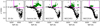 |
Fig. 1. Member selection in the γ vs Teff plane for the five clusters in our sample. The magenta lines indicate the exclusion region we adopted for the selection. Stars marked with green diamonds have been excluded as contaminants. |
For stars observed only with UVES, we excluded all objects with log g < 3.5 dex and 4000 K < Teff < 5500 K. This selection was also applied to stars observed with Giraffe with an available log g value to reject a few residual giants that could not be identified using the γ index.
3.2. Radial velocity and astrometry
Figure 2 shows the RV versus parallax and the proper motion diagrams of the GES samples of the five clusters after the gravity selection. The 25 Ori cluster is the group of stars at RV ∼ 20 km s−1, ϖ ∼ 2.9 mas, and  . The other smaller group at
  is the secondary population (Zari et al. 2019), which corresponds to the group of stars around RV ∼ 30 km s−1. The two populations of Gamma Vel (Jeffries et al. 2014) can be clearly identified in both diagrams. Gamma Vel A is concentrated at RV ∼ 17 km s−1, ϖ ∼ 2.9 mas, and
  , and Gamma Vel B is distributed along a more elongated structure (see Franciosini et al. 2018). In the case of NGC 2547, the B population from Sacco et al. (2015) can be seen as a distinct, small group of stars at RV ∼ 20 km s−1 and
  . The diagrams for NGC 2451 show that the two clusters are very well separated in all parameters: NGC 2451 B is the group with lower RV, parallax, and total proper motion. NGC 2516 shows a single peak without evidence for additional populations.
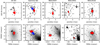 |
Fig. 2. GES RV versus parallax (top panels) and proper motion diagrams (bottom panels) for the GES samples for the five clusters after the gravity selection (black dots). In the proper motion diagrams we also plot the density map of the full Gaia samples on a grey scale. The final samples of selected GES and Gaia members are overplotted as red and light red dots, respectively, for 25 Ori, Gamma Vel A, NGC 2451 B, NGC 2547 and NGC 2516, and as blue and light blue dots, respectively, for Gamma Vel B. |
Figure 2 clearly shows that the samples still contain a significant number of field contaminants. This is particularly true for the Gaia samples, in which the number of background sources is extremely large. To remove the bulk of contaminants and reduce the samples to manageable sizes, we used the GES samples to derive first-guess average centroids and standard deviations of the parallaxes and proper motions for each population, applying a 3σ clipping. We then excluded all stars with reliable astrometry from the full samples that lie at more than 5σ from these centroids, taking the individual errors into account. That is, we retained only stars satisfying the following relation:
 (1)
(1)
for at least one cluster population. Adopting a higher threshold would significantly increase the number of field objects, especially for the younger clusters. This would complicate the fit described below and increase the risk of including contaminants in our final samples. For NGC 2547, we considered only the main cluster and discarded the secondary population since it cannot be constrained by the fit. For 25 Ori we kept both populations for the fit, although only members of the main cluster were selected afterwards. Because the two NGC 2451 clusters are well separated in all parameters, it might be possible in principle to select only stars around the centroid of cluster B, but the GES sample contains a significant number of stars lacking reliable astrometry (to which the above selection therefore cannot be applied) but with an RV that is consistent with that of NGC 2451 A. For this reason, we preferred to fit the data for both clusters and then selected the members of NGC 2451 B afterwards.
For each cluster, we performed a simultaneous fit of the distributions of RVs, parallaxes, and proper motions for the reduced datasets using a maximum likelihood approach and assuming that the total probability distribution is described by the sum of one or two cluster populations plus the field. To do this, we extended the method described by Lindegren et al. (2000) that was used by Franciosini et al. (2018) and Roccatagliata et al. (2018) and included the RV as a fourth parameter. A detailed description is given in Appendix A. The resulting best-fit values for the cluster components are given in Table 1. Individual membership probabilities Pi for each population were derived using the standard method, that is, dividing the probability of belonging to the given population by the total probability. For the following analysis, we selected only the highest-probability members of each cluster population with Pi > 0.96.
Maximum likelihood best-fit parameters of the RV and astrometry distributions of the sample clusters.
3.3. Parallax zero-point correction
Lindegren et al. (2021b) investigated the systematic bias affecting Gaia EDR3 parallaxes, which shows a complex dependence on magnitude, colour, and ecliptic latitude, and provided a tentative correction for the parallax zero-point. Fabricius et al. (2021) showed that applying this correction to distant clusters improves their parallax distribution reducing the internal dispersion. Hence, we tested the effect of the bias correction on our results.
The zero-point for each star was computed using the Python code provided on the Gaia web pages4, and the whole analysis of Sect. 3.2 was repeated using the corrected parallaxes. For all clusters, we found no significant difference in the best-fit parameters, except for the central parallax, or in the list of selected members. The mean parallax is increased by 0.026 − 0.039 mas, depending on the cluster. In the following, we therefore adopt the results of Sect. 3.2, although we discuss the effect of this parallax bias on the model comparison.
3.4. Photometry and lithium
As a final step, we examined the photometry and the lithium abundances to identify possible residual contaminants in our samples. The sequences of the selected high-probability members with reliable photometry are very clean in the G versus G − GRP CMD. However, we found one star in Gamma Vel B and one in NGC 2451 B that lay more than 1 mag below the cluster sequence. These objects were discarded from the samples. Similarly, we discarded one star in 25 Ori and one in NGC 2547, both with Teff ∼ 5300 K and lithium ∼2 dex below the lower envelope of the cluster sequences in the A(Li) vs Teff diagrams, since these are likely to be non-members.
3.5. Final members
The selection procedure described above allowed us to obtain very clean lists of secure members, which are fundamental for a precise comparison with theoretical models. The final membership lists contain 442 members of 25 Ori (137 GES), 325 members of Gamma Vel A (118 GES), 128 of Gamma Vel B (44 GES), 255 of NGC 2547 (146 GES), 125 members of NGC 2451 B (42 GES), and 536 of NGC 2516 (363 GES). Their properties are listed in Tables B.1–B.6.
The CMDs and lithium patterns of the final members are plotted in Fig. 3. All clusters show very clean sequences, although some scatter is still present, especially at the lowest masses. For some of them, the binary sequences are also well distinguished. The bright end of the NGC 2516 sequence shows a significant spread. This might be indicative of an extended main-sequence turn-off, which has recently been observed in Galactic open clusters of different ages (e.g. Bastian et al. 2018; Marino et al. 2018; Li et al. 2019, and references therein), and is generally attributed to a spread in rotation rates. Unfortunately, we do not have information on rotation for these stars that could confirm this hypothesis.
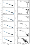 |
Fig. 3. CMDs (left panels) and lithium distribution as a function of Teff (right panels) of the final samples of selected members for each cluster. The GES and Gaia members are indicated by black and blue dots, respectively. Left panels: only stars with good photometry are plotted. The errors on photometry are smaller than the symbol size. Downward triangles in the lithium diagrams indicate upper limits. |
The right panels of Fig. 3 show the evolution of the lithium abundances with age. The lithium depletion pattern of 25 Ori is very similar to the pattern observed in Gamma Vel A and B (Jeffries et al. 2014), with a continuous range of lithium abundances for stars between ∼3200 and ∼3600 K, from nearly undepleted stars to fully depleted ones. To our knowledge, this is the first determination of the lithium depletion pattern in 25 Ori. The similarity with Gamma Vel suggests that these clusters have similar ages and that this particular depletion pattern is a common characteristic of young clusters at this age. At the age of NGC 2451 B and NGC 2547, M-type stars are generally fully depleted, although some of them still retain some amount of lithium; we also note the start of the lithium increase at the LDB that is clearly visible in NGC 2547. At the age of NGC 2516, lithium depletion has proceeded to higher masses, although a strong scatter is present. Several stars retain a significant amount of lithium even below 4000 K.
The younger clusters include some stars, between ∼4800 and 6000 K, whose lithium abundance is significantly higher than the initial cosmic abundance A(Li) ∼ 3.3 (e.g. Martín et al. 1994; Romano et al. 2021). This is a signature of non-local thermodynamic equilibrium (NLTE) effects: if the three-dimensional NLTE corrections by Wang et al. (2021) were applied, these abundances would be reduced by ∼0.3−0.4 dex, bringing them in agreement with the cosmic value. At higher temperatures, the corrections are not significant, being < 0.1 dex. However, the Wang et al. (2021) grid is limited to Teff ≥ 4000 K and does not cover the full range of temperatures in our samples. For this reason, the corrections were not applied to our data. The high lithium abundance of the two stars at 3000 K in 25 Ori is instead likely caused by an underestimated gravity due to the low signal-to-noise ratio of the spectra: their reported log g is ∼3.2−3.4 dex, but their γ index and spectra indicate that they are dwarfs. A more reasonable value of log g = 4.0 dex would lower their abundances to ∼3.3.
4. Comparison with evolutionary models
4.1. Models
The models were calculated with the Pisa evolutionary code (Tognelli et al. 2011; Dell’Omodarme et al. 2012). The main input physics and parameters are described in detail in Tognelli et al. (2015a,b, 2018). Here we only point out some relevant characteristics and some improvements with respect to the quoted works.
The adopted radiative opacity tables are OPAL 20055 (Iglesias & Rogers 1996) for the stellar interiors and Ferguson et al. (2005)6 for the most external regions, both computed for the Asplund et al. (2009) solar mixture. The equation of state is the OPAL 2006 (Rogers & Nayfonov 2002), consistent with the adopted opacities, extended to the low-mass star regime (M ≲ 0.2 M⊙) by the Saumon et al. (1995) equation of state.
Convective transport in super-adiabatic regions was treated following the mixing length formalism by Böhm-Vitense (1958), where the convection efficiency is expressed in terms of the mixing length scale ℓML = αML HP, where αML is the mixing length parameter and HP is the pressure scale height. As reference value we adopted our solar-calibrated7 parameter αML = 2.0. This value was shown to reproduce the CMD of the Hyades cluster well (Tognelli et al. 2021b). In addition, to test the effect of a reduced convection efficiency on the models, we also considered the two cases αML = 1.0 and 1.5.
The most relevant nuclear reactions for our analysis are the hydrogen-burning reactions, that is, the pp-chain and the CNO-cycle. Their reaction rates are from Adelberger et al. (2011), except for p(p,e+ν)2H, which is from Marcucci et al. (2013) and Tognelli et al. (2015b), 2H(p,γ)3He, which is from Descouvemont et al. (2004), 7Li(p,α) α, which is from Lamia et al. (2012), and p(14N,γ)15O, which is from Imbriani et al. (2005).
We obtained the outer boundary conditions from the detailed non-grey BT-Settl atmospheric structures8 by Allard et al. (2011) for Teff ≲ 10 000 K and from the Castelli & Kurucz (2003) structures for higher Teff. We also included the possibility in the models of having a partial coverage of the stellar surface by starspots, which block part of the outgoing radiation. To model the spots, we used a formalism similar to that described in Somers & Pinsonneault (2015). We treated the spots as a pure surface effect, assuming that they do not extend below the stellar surface, that is, that the spot scale height is much smaller than the pressure scale height. The total luminosity at the stellar surface is given by the following expression:
 (2)
(2)
where βspot is an effective spot coverage fraction, which takes the ratio of the spot and stellar surface effective temperature and the real fraction of area covered with spots into account. This is defined as
 (3)
(3)
The parameter βspot is useful when information about the real spot coverage 𝒜spotted/𝒜⋆ or on Tspot/Teff is not well constrained. In these cases, it is sufficient to specify only the effective spot coverage instead of requiring two free parameters (namely Tspot/Teff and 𝒜spotted/𝒜⋆). For the typical values of Tspot/Teff ∼ 0.7 − 0.9 observed in active stars (e.g. Berdyugina 2005, and references therein), βspot ∼ 0.76 − 0.34 𝒜spotted/𝒜⋆. We analysed the effect of two different values of effective spot coverage on the models, namely βspot = 0.20 and 0.40, which are consistent with those suggested by recent observations of late-type stars (e.g. Fang et al. 2016; Gully-Santiago et al. 2017; Morris et al. 2019).
For a star with a given luminosity and effective temperature, the radius of a spotted model is  , which is larger than the radius of the corresponding unspotted model. The effective surface that can freely radiate the energy is reduced by a factor (1 − βspot), and consequently, the total surface of the star has to increase by the same factor to keep the luminosity constant.
As mentioned in Sect. 1, all the clusters present in our sample are fully compatible with a solar chemical composition, that is, [Fe/H] = 0. Using the Asplund et al. (2009) relative metal abundances, a helium-to-metal enrichment ratio ΔY/ΔZ = 2 (Tognelli et al. 2021b), and a primordial helium abundance Yp = 0.2485 (Cyburt 2004; Aver et al. 2012, 2013), we obtained an initial helium and global metallicity Y = 0.2740 and Z = 0.0130, respectively. Concerning light elements, we set the mass fractional abundance of deuterium to XD = 2 × 10⁻⁵, which is representative of the present Galactic D abundance (Linsky et al. 2006; Sembach 2010), and the initial 7Li abundance to reproduce that measured in stars with Teff > 6000 K, where lithium is still undepleted. For all cases, we adopted a value of A(Li) = 3.3, which is consistent with the average initial abundance of young open clusters derived by Romano et al. (2021) using GES iDR6 data.
Evolutionary tracks were computed in the mass interval [0.06, 10] M⊙ with a variable mass spacing. From these tracks, we calculated the isochrones in the age interval [0.5, 200] Myr. Theoretical isochrones were converted into Gaia EDR3 magnitudes using the filter response curves given in Riello et al. (2021) and computing the bolometric corrections using the MARCS 2008 atmospheres (Gustafsson et al. 2008) for Teff ≤ 8000 K and the Castelli & Kurucz (2003) ones for higher Teff.
Figure 4 shows the comparison between the isochrones at 15, 30, and 100 Myr (representative of our cluster sample) obtained for the standard set of models (αML = 2.0) for the sets with a smaller mixing length parameter (αML = 1.0 and 1.5) and without spots, and the sets with αML = 2.0 and βspot = 0.2 and 0.4. The effects on the CMD are shown in the top panels of Fig. 4. As is well known, a variation in αML mainly affects the colours of stars with thick and superadiabatic envelopes, therefore its effect depends on stellar mass. Very low-mass stars are fully convective but almost adiabatic, and thus they are not sensitive to the adopted αML. As the mass increases, the outermost layers of the star become superadiabatic, but the convective envelope becomes increasingly thinner as the mass increases. As a result, the effect of varying αML is maximum in an intermediate mass interval. Conversely, the effect of spots increases as the stellar mass decreases, producing significantly redder isochrones for M-type stars: this happens because spots modify the outer boundary conditions, which become increasingly more important as the mass decreases (see e.g. Tognelli et al. 2011, 2018).
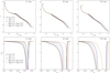 |
Fig. 4. Effect of adopting different values of αML and of different spot coverage fractions on the models at 15 Myr (left panels), 30 Myr (middle panels), and 100 Myr (right panels). The top row shows the effect on the CMD, and the bottom row presents the effect on the surface lithium abundance as a function of Teff. The standard reference model with αML = 2 and no spots is plotted as the solid black line. The dashed red and dot-dashed blue lines show the models without spots and αML = 1.5 and 1.0, respectively. The models with αML = 2 and βspot = 0.2 and 0.4 are indicated with the dotted green and three-dot-dashed orange lines, respectively. |
The bottom panels of Fig. 4 show the surface lithium abundance as a function of the effective temperature for the selected ages. The LDB is clearly visible in all panels. As is well known, as the age increases, the LDB moves to lower temperatures and its luminosity decreases (see e.g. Tognelli et al. 2015a). The effect of αML and βspot on the surface lithium abundance is more evident than that on the CMD. By reducing αML or increasing βspot, the models become cooler and lithium is less efficiently destroyed.
The two parameters αML and βspot affect the models in different ways. As mentioned before, a variation in αML changes the structure only in a limited mass interval. For very low-mass stars (i.e. almost adiabatic ones, for Teff ≲ 3500 K), the variation in αML has a negligible effect on Teff and on the lithium burning, which results in no significant change of the LDB. On the other hand, for higher masses (3500 K ≲ Teff ≲ 6500 K), the structure and lithium burning are affected by a change in αML, and this produces a shift in the left side of the lithium ‘chasm’ (Basri 1997) towards lower temperatures as αML decreases. In contrast, a change in βspot affects all stars with Teff ≲ 6500 K and moves not only the hot side of the chasm, but also moves the LDB slightly towards lower temperatures as βspot increases. Furthermore, the amount of lithium depletion in the chasm significantly decreases as the spot coverage increases at 15 Myr, and the LDB may not be clearly defined. The inclusion of spots also affects the luminosity of the model at the LDB, and consequently, its derived age. Somers & Pinsonneault (2015) estimated an increase in LDB age of about 13−15% in the age interval 15−30 Myr, assuming a (real) coverage fraction fspot = 0.59. Our model grid was not computed with the aim to provide LDB models, and it is not dense enough in mass to allow a precise identification of the LDB at young ages, as was done in Tognelli et al. (2015a). Nevertheless, we estimate that the age increases by approximately 8−10% at 15−30 Myr and ∼6% at 100 Myr in the case of βspot = 0.2, while the relative age increase is about 20−24% at 15−30 Myr and 15% at 100 Myr for βspot = 0.4. Similar variations were found by Binks et al. (2021) from their analysis of the LDB in NGC 2232. Therefore, the very different effects produced by the two parameters αML and βspot on the lithium pattern should allow us at least in principle to distinguish which one of them is dominant.
4.2. Determination of cluster reddening and age
The age and reddening E(B − V) for each cluster were derived using the Bayesian maximum likelihood method described in Randich et al. (2018) and Tognelli et al. (2021b) (see also Hatzidimitriou et al. 2019). The analysis is based on a star-by-star comparison of the observed Gaia EDR3 magnitudes with our theoretical isochrones. The age and E(B − V) were derived by constructing a two-dimensional likelihood: the likelihood peak was used to obtain the best value while the uncertainty was evaluated by marginalising the distribution and finding the regions in its wings that account for 16% of the total area. To perform the analysis, we used a combination of all three Gaia magnitudes, considering in particular the plane (G − GRP, GBP). We selected only stars with an absolute GBP magnitude lower than 7.5 (corresponding to about 0.7−0.8 M⊙ for ages older than 20−30 Myr). In this region, models and observation attain a satisfactory agreement. At higher magnitudes (in particular for G − GRP ≳ 0.9), some problems persist (not well understood) that prevent a good agreement between models and data, such as difficulties in the modelling of synthetic spectra at solar and supersolar metallicities, or in predicting the radius/Teff relation in fully convective PMS low-mass stars (see e.g. Kučinskas et al. 2005; Gagné et al. 2018; Tognelli et al. 2021b). We therefore decided to exclude this part of the data from the recovery to avoid introducing an uncontrollable bias. We also excluded stars that lie on the binary sequence or that are clearly outliers from the fit.
To evaluate the uncertainties on the results, we took the errors coming from the photometry (mean Δ(G − GRP) and ΔGBP ∼ 2 − 5 mmag) and the systematic parallax bias of ∼0.03 mag derived in Sect. 3.3 into account. The impact of the zero-point correction is small: it accounts for an uncertainty of about 3−5 mmag in E(B − V) and an age increase of 1−2 Myr.
If the stars have the same physical parameters and the photometric errors are reliable, we would expect them to lie on the same isochrone. However, the CMDs show that this is not the case (see Fig. 3), as in all clusters a scatter larger than the observable errors is present. This could mean that some additional mechanisms, different from star to star, might play a non-negligible role. Hence, we only aim to reproduce the average characteristics of the stellar population in our comparison.
The procedure was applied to different sets of models: (i) the reference case with solar-calibrated mixing length (αML = 2.0) without spots, (ii) the sets with αML = 1.0 and αML = 1.5 without spots, and (iii) the sets with αML = 1.0, 1.5, and 2.0 and βspot = 0.2 and 0.4.
The recovery of the age and reddening was performed as follows: we first derived the age and reddening of each cluster for the reference case. The reddening was mainly determined by the comparison between theory and observation of the zero-age main-sequence (ZAMS) portion of the cluster sequence because its position in the CMD is independent of age. This region is populated by stars without a convective envelope that are not affected by variations in the mixing length or by surface spots. Therefore the reddening can be derived independently of the considered model set. For this reason, we fixed the reddening to that derived using the reference set to save computational time. On the other hand, the estimated age changes using different sets of models because it is derived from the PMS low-mass stars, which have convective envelopes, thus their position in the CMD changes if αML varies and if surface spots are included or excluded. These clusters do not have enough stars in the turn-off region to allow an age determination from the hydrogen exhaustion luminosity.
After the age and reddening for each cluster and each set of models were derived from the Bayesian fitting of the CMD, we extracted the corresponding lithium isochrones and compared them with the observed lithium depletion pattern. This allowed us to identify the model that better reproduces the data and to consequently determine the best cluster age. The observed lithium abundances show too much scatter to allow the use of the Bayesian maximum likelihood method to derive the characteristics of the best-fit model. We also note that if magnetic phenomena are present, they are expected to show a distribution of their efficiencies among the cluster stars, and this could strongly contribute to the observed dispersion. In this case, lithium observations cannot be fitted by a single isochrone, but the set that best reproduces the average lithium profile can still be identified. The model parameters given in Table 2 (and the corresponding isochrones plotted in Figs. 5–8) reproduce the CMD and the position of the lithium chasm best. The observed spread in the observed lithium abundances inside the chasm is too large in most cases to be reproduced by a single isochrone with a defined set of parameters.
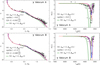 |
Fig. 5. Comparison of the data with the best-fit model in the CMD (left panels) and in the lithium–Teff plane (right panels) for Gamma Vel A (top) and Gamma Vel B (bottom). Errors on photometry are smaller than the symbol size. Open downward triangles in the lithium diagrams represent upper limits for A(Li). The best-fit model with αML = 1.0 and βspot = 0.2 is shown as a solid blue line, and the isochrones corresponding to the maximum and minimum age derived by the fitting method are shown as dashed and dot-dashed red lines, respectively. The long-dashed green line is the isochrone at the same age, reddening, and αML as the best-fit model, but with βspot = 0. |
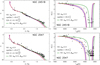 |
Fig. 7. Same as Fig. 5 for NGC 2451 B (top) and NGC 2547 (bottom). In this case, the best-fit model (solid blue line) corresponds to αML = 2.0 and βspot = 0. The long-dashed green line shows the isochrone with the same age, reddening, and αML as the best-fit model, but computed with βspot = 0.2. |
Best-fit model parameters for each cluster.
4.3. Gamma Vel A and B
The best-fit models for Gamma Vel A and Gamma Vel B are shown in Fig. 5. In both cases, the best agreement with the observations is obtained when the effect of the magnetic field both on the stellar interior, with a reduced convection efficiency αML = 1.0, and on the surface, with a 20% effective spot coverage, is considered. In particular, βspot = 0.2 is required to reproduce the correct position in Teff of the lithium depletion region. Lower or higher values of βspot in fact shift the position of the chasm towards higher or lower temperatures, respectively, as shown in Fig. 4. Higher values of αML result in significantly younger best-fit ages and lower lithium depletion than observed. We note, however, that as mentioned before, the abundance spread in this region is large and cannot be reproduced using a single isochrone with a fixed parameter set.
In the case of Gamma Vel A, we derive a reddening  mag and an age of
  Myr. The best-fit model can satisfactorily reproduce the average data distribution in the CMD and the lithium–Teff plane. However, the lithium diagram shows a significant discrepancy at Teff ∼ 3700 − 4300 K, where the data show much more lithium depletion than predicted. This might suggest that magnetic effects in these stars are less efficient. To verify this hypothesis, we also plot in Fig. 5 the isochrone with αML = 1.0 and the same age and reddening as the best-fit one but without spots. A range of spot coverage between 0 and 0.2 could explain the observed higher depletion level at least below 4000 K, including the depth of the depletion pattern. In particular, the hottest of the strongly depleted stars appear to coincide with the boundary for βspot = 0. This model also seems to provide a better fit to part of the stars in the CMD for G − GRP = 0.5 − 0.9. However, even the model without spots is not able to completely solve the disagreement above 4000 K. The reason for this is not clear and deserves further investigation in future works. In addition to this, also stars around ∼3200 K appear to be slightly more depleted than the prediction of the best-fit model. These stars could be reproduced assuming a higher spot coverage, up to βspot = 0.4 (not shown in Fig. 5, but see Fig. 4, bottom left panel).
We find similar results for Gamma Vel B. For this cluster we derive a reddening  mag and an age of
  Myr. The central age for Gamma Vel B is slightly older than the age derived for Gamma Vel A, but it is consistent within the uncertainties, therefore the two populations could be coeval. The lower number of stars available for this cluster is responsible for the higher uncertainty on the best-fit age. Similarly to the previous case, we find that the model and the mean data distribution for the CMD and the lithium pattern agree well. In particular, the model can reproduce the position in Teff of the lithium depletion region very well. As for Gamma Vel A, a mix of stars with different starspot coverage (from no spots to βspot = 0.2) is able to reproduce the observed spread in lithium between ∼3500 and ∼4000 K.
We note that, while for both clusters the agreement in the CMD is very good for G − GRP ≲ 0.9 − 1, the best-fit model for cooler stars does not provide a perfect match to the cluster sequences, being consistent with their lower envelope. This discrepancy could in part be due to the presence of stars with higher spot coverages, as suggested by the lithium pattern, which would make them redder. As mentioned in Sect. 4.2, however, there might be other potential effects that are not well understood so far, that might also play a role and might partly contribute to the discrepancy.
Our results agree very well with what was found by Jeffries et al. (2017), who showed that models with inflated radii from magnetic inhibition of convection or starspots are required to simultaneously reproduce the CMD and lithium pattern of Gamma Vel A and B at an age of 18−21 Myr. However, Jeffries et al. (2017) did not distinguish between the two populations. To our knowledge, ours is the first precise determination of the ages and reddening of Gamma Vel A and B separately.
4.4. 25 Ori
Figure 6 shows the best-fit isochrone for the 25 Ori cluster. As in the case of Gamma Vel A and B, the best agreement in the CMD and the lithium–Teff plane is obtained using the models with αML = 1.0 and βspot = 0.2. We derive an age of  Myr and a reddening
  . This places this cluster in the same age range as Gamma Vel A and B, as expected from the very similar lithium pattern. As already found for Gamma Vel, the age derived using magnetic models is much higher than the values derived previously from simple isochrone fitting with standard models, which range from 6.1 ± 0.8 Myr (Downes et al. 2014) to 13.0 ± 1.3 Myr (Kos et al. 2019). The best fit with our standard model would give an age of 12 Myr, consistent with previous determinations, but this model would not be able to reproduce the observed lithium pattern.
As already observed in the previous section, the best-fit model alone is not able to completely reproduce the lower-mass part of the CMD and the observed abundance spread in this case either. In particular, several stars around 3600 − 4000 K are more depleted than predicted by the best-fit isochrone. These stars could be reproduced assuming a range of spot coverages between 0 and 0.2, while higher spot coverage fractions could better explain the abundances of the coolest stars, as in Gamma Vel A.
4.5. NGC 2451 B and NGC 2547
Figure 7 shows the best-fit results for the two nearly coeval clusters NGC 2451 B and NGC 2547. In both cases, the model that provides the best agreement with the data in the CMD and the lithium–Teff plane is the model with solar-calibrated mixing length, that is, αML = 2.0, without spots. Models with reduced convection efficiency are not able to reproduce the lithium pattern at Teff ≳ 4000 K because they provide too little lithium depletion.
In the case of NGC 2451 B, we derive a reddening  mag and an age of
  Myr, in agreement with the recent results by Randich et al. (2018). This cluster has a limited number of members as well, which prevents a precise age determination. Nevertheless, the agreement with the observations is very good throughout the entire CMD sequence, except for the very low-mass tail. For NGC 2547 we derive a reddening
  mag and an age of
  Myr, consistent with the LDB age derived by Jeffries & Oliveira (2005) and with other previous studies (e.g. Naylor & Jeffries 2006; Randich et al. 2018). Similarly to NGC 2451 B, standard isochrones provide the best fit to the CMD, except at very low masses. The standard model also reproduces the lower envelope of the lithium depletion pattern in both clusters well, as well as the position of the LDB in NGC 2547. As mentioned in Sect. 3.5, however, both clusters show significant scatter, and several stars are less depleted than expected. This scatter, as well as the low-mass tail in the CMD, could be accounted for if these stars were still affected by a non-negligible magnetic effect, which in such low-mass stars is reflected only in a certain percentage of spot coverage. Figure 7 indeed shows that the isochrone with the same age, reddening, and αML as the best-fit isochrone, but with βspot = 0.2, provides a better match to the lower cluster sequences and can successfully reproduce the upper envelope of the lithium pattern for both clusters. The spotted model can also account for the small spread observed among the stars at the LDB in NGC 2547.
In NGC 2547 some stars at lower temperatures inside the chasm still retain some lithium, in contrast to what is expected from the models. It is possible that these stars are more magnetically active and have a larger spot coverage, which would lead to a lower depletion efficiency. We note, however, that lithium measurements of strongly depleted stars at these low temperatures are difficult because of the significant blending with molecular bands. Therefore we cannot exclude that the observed scatter might at least in part be due to uncertainties in the measures.
4.6. NGC 2516
NGC 2516 is the oldest cluster in our sample. We derive an age of  Myr and a reddening
  mag using the solar-calibrated isochrones (Fig. 8). The age and reddening we found are consistent with the values given in the literature (see e.g. Jeffries et al. 1998; Sung et al. 2002; Lyra et al. 2006; Randich et al. 2018, and references therein). With the exception of the low-mass tail, the CMD is reproduced very well. The age in this cluster is derived mainly from turn-off stars, as low-mass stars are on the ZAMS and consequently, their position is independent of age. Unfortunately, as noted in Sect. 3.5, bright stars show a significant photometric scatter, so that the derived age uncertainty is quite large. The standard model isochrone also agrees well with the bulk of the lithium distribution for Teff ≳ 4500 K, although significant scatter is present below ∼5000 K. This scatter can be accounted for by assuming a distribution of the spot coverage among the cluster stars between 0 and 20%. In particular, the model with βspot = 0.2 provides a good match to the upper envelope of the lithium pattern above ∼4000 K. This model also appears to better reproduce the low-mass tail of the CMD, similarly to NGC 2451 B and NGC 2547. In this case as well, a number of cooler stars has much higher lithium abundances than predicted by the models. This might be reproduced by assuming a higher spot coverage fraction.
5. Discussion and conclusions
Observations of field and cluster stars suggest that effects due to magnetic activity, which can reduce the external convection efficiency and produce a significant coverage of the stellar surface with spots, might be present. In this paper, we modelled these effects in a consistent way including them in the Pisa stellar evolutionary code. The code was used to calculate cluster isochrones and to predict the time behaviour of the surface lithium abundance. Theoretical predictions were compared with the observed CMDs and lithium abundance patterns of five young open clusters of different ages, taking advantage of the homogeneous stellar parameters and lithium abundances provided by GES, and of the precise astrometry and photometry from the Gaia EDR3 release. The quality of the combined GES and Gaia data allowed us to gain important insights into PMS evolution.
Lithium data place strong constraints on the best set of models (see also Jeffries et al. 2021). As shown in the previous section, lithium depletion strongly depends on a change in αML and βspot and, more importantly, the effects of these parameters are different. Intermediate-mass stars are affected by a variation in the convection efficiency, but are insensitive to spots. On the other hand, in low-mass stars, which are almost adiabatic, lithium abundances are not affected by a variation in αML, but strongly depend on the adopted effective spot coverage. This differential sensitivity allows us to distinguish among models that were computed with different assumptions on these parameters.
From the analysis of the lithium abundance patterns and the CMDs of our sample of young open clusters, the following picture seems to emerge:
-
For clusters younger than ∼20 Myr, we confirm that standard models cannot simultaneously reproduce the observed CMD and the lithium pattern, as already noted by Jeffries et al. (2017) for Gamma Vel. These clusters can be reproduced using models that include both a non-negligible spot coverage and a reduced super-adiabatic convection efficiency in the stellar envelope. In particular, a mix of different spot coverages in different stars that increase with decreasing mass appears to be necessary to explain the observed lithium depletion pattern.
-
In older clusters (i.e. ages older than ∼30−40 Myr), standard isochrones provide a good agreement with the data. However, low-mass stars in these clusters show a significant discrepancy with the models in both the CMD and the lithium pattern. This discrepancy can be reduced when models with spots are considered. Spotted models can not only explain the observed lithium dispersion in NGC 2451 B, NGC 2547, and NGC 2516, in particular the large spread at Teff ∼ 3200 − 3800 K, but they also provide a better fit to the low-mass tail in the CMD. The value of βspot = 0.2 that best reproduces the low-mass cluster sequences and the upper envelope of the lithium patterns is consistent with the 34% real spot coverage found by Jeffries et al. (2021) to reproduce the lithium upper envelope in M 35, assuming Tspot/Teff = 0.8.
Magnetically active stars are well known to exhibit spots covering a significant fraction of their surface. Recently, Fang et al. (2016) investigated the spot distribution of low-mass stars in the Pleiades, finding a large spread, from no spots to high coverage fractions: the upper envelope of this distribution increases from G- to M-type stars, up to maximum values of effective coverage ∼0.3 for stars in the saturated regime. However, the spread in spot coverage is present even in the saturated regime for stars with Teff ≤ 3800 K. These results strongly support our hypothesis that the lithium dispersion might be due to the presence of stars with different spot coverage fractions that increase at lower masses.
As a further verification, we investigated whether the lithium abundances are correlated with magnetic activity. It is well known that magnetic activity increases with increasing rotation rate (or equivalently, decreasing Rossby number Ro) up to a saturation level corresponding to Ro ≲ 0.1 (e.g. Pizzolato et al. 2003). A correlation between lithium and rotation has long been known to exist in the Pleiades (Soderblom et al. 1993; Somers & Stassun 2017) and has also been observed in other clusters even at very young ages (e.g. Bouvier et al. 2016; Jeffries et al. 2021). In Fig. 9 we show the lithium abundances as a function of the chromospheric Hα emission log L(Hα)/Lbol, which was computed from the measured chromospheric Hα flux available in the GES catalogue. In the case of NGC 2516, we also show lithium as a function of the Rossby number provided by Fritzewski et al. (2020). For the three younger clusters we simply plot the measured A(Li) for stars between 3000 and 3700 K. For the older clusters, we instead computed the difference ΔA(Li) between the observed abundance and that predicted by the best-fit standard model for stars between 3000 and 6000 K (excluding those close to the LDB), assuming the value A(Li) = −1 for complete depletion, which is consistent with the minimum value measured in GES. Stars that should be fully depleted according to the model are marked with red symbols in Fig. 9. The lithium excesses for fully depleted stars should be regarded as lower limits because their true abundance could be lower than our assumed minimum value. We find a clear correlation with chromospheric activity and Rossby number for NGC 2516: the lithium excess increases with decreasing Ro and increasing log L(Hα)/Lbol, and stars with the highest excess, including the undepleted M-type stars, all have Ro ≲ 0.1, that is, they are saturated. In the younger clusters, all the M-type stars have saturated levels of Hα emission, implying that they have strong magnetic activity.
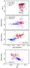 |
Fig. 9. Lithium as a function of the chromospheric activity indicator log LHα/Lbol for detections only (top three panels). First panel: A(Li) for stars with 3000 < Teff < 3700 K in Gamma Vel A (open black circles), Gamma Vel B (open blue squares) and 25 Ori (red stars). Second and third panels: lithium excess ΔA(Li) (see text) for stars with 3000 < Teff < 6000 K in NGC 2451 B and NGC 2547 (second panel, open circles and squares, respectively), and NGC 2516 (third panel, open circles). The red symbols mark stars for which the models predict full lithium depletion. Bottom panel: ΔA(Li) for NGC 2516 members as a function of the Rossby number Ro from Fritzewski et al. (2020). The symbols are the same as in the third panel. |
In conclusion, models including the effects of magnetic activity, such as starspots, seem able to provide a consistent explanation of the low-mass cluster sequences and of the lithium abundance patterns observed in young clusters. The observed dispersion in the lithium abundances could be the result of different star-to-star spot coverage fractions. However, some inconsistencies are still present, both at the lower-end of the CMD and between the predicted and observed lithium pattern. A possible improvement could be attained by introducing a mass-dependent spot coverage, or a variation in the spot coverage in time due to the evolution of rotation in low-mass stars. We cannot exclude either that some other mechanism may play a role in producing part of the observed lithium dispersion. This requires further investigation and a comparison with a larger sample of young open clusters.
In the usual notation A(Li) = log N(Li)/N(H)+12.
These are sources without prior reliable colour information, for which an additional pseudo-colour parameter was required for the astrometric solution (see Gaia Collaboration 2021).
Our standard solar model was computed using an iterative procedure in which the initial helium abundance, metallicity, and mixing length parameter were adjusted to reproduce the observed radius, luminosity, and photospheric (Z/X) in a 1 M⊙ model at the solar age within a given numerical tolerance (< 10−4).
Somers & Pinsonneault (2015) assumed a value of Tspot/Teff = 0.8 and a maximum value of fspot = 𝒜spotted/𝒜⋆ = 0.5. Their models with fspot = 0.5 correspond to our value of βspot ≈ 0.3.
For the fit, we adopted the SLSQP minimisation method as implemented in scipy.
Acknowledgments
We thank E. Martin for his fruitful comments as referee of this paper. Based on data products from observations made with ESO Telescopes at the La Silla Paranal Observatory under programmes 188.B-3002, 193.B-0936, and 197.B-1074. These data products have been processed by the Cambridge Astronomy Survey Unit (CASU) at the Institute of Astronomy, University of Cambridge, and by the FLAMES/UVES reduction team at INAF/Osservatorio Astrofisico di Arcetri. These data have been obtained from the Gaia-ESO Survey Data Archive, prepared and hosted by the Wide Field Astronomy Unit, Institute for Astronomy, University of Edinburgh, which is funded by the UK Science and Technology Facilities Council. This work was partly supported by the European Union FP7 programme through ERC grant number 320360 and by the Leverhulme Trust through grant RPG-2012-541. We acknowledge the support from INAF and Ministero dell’Istruzione, dell’Università e della Ricerca (MIUR) in the form of the grant “Premiale VLT 2012”. The results presented here benefit from discussions held during the Gaia-ESO workshops and conferences supported by the ESF (European Science Foundation) through the GREAT Research Network Programme. We acknowledge the support from INAF in the form of the grant for mainstream projects “Enhancing the legacy of the Gaia-ESO Survey for open clusters science”. E.T. acknowledges Czech Science Foundation GAR (Project: 21-16583M) and the “visiting fellow program” of the University of Pisa. P.G.P.M. and S.D. acknowledge INFN (Iniziativa specifica TAsP). E.P. and N.S. acknowledge financial support from Progetto Main Stream INAF “Chemo-dynamics of globular clusters: the Gaia revolution”. R.B. acknowledges financial support from the project PRIN-INAF 2019 “Spectroscopically Tracing the Disk Dispersal Evolution”. F.J.E. acknowledges financial support from the Spanish MINECO/FEDER through the grant AYA2017-84089 and MDM-2017-0737 at Centro de Astrobiología (CSIC-INTA), Unidad de Excelencia María de Maeztu, and from the European Union’s Horizon 2020 research and innovation programme under Grant Agreement no. 824064 through the ESCAPE – The European Science Cluster of Astronomy & Particle Physics ESFRI Research Infrastructures project. This work has made use of data from the European Space Agency (ESA) mission Gaia (https://www.cosmos.esa.int/gaia), processed by the Gaia Data Processing and Analysis Consortium (DPAC, https://www.cosmos.esa.int/web/gaia/dpac/consortium). Funding for the DPAC has been provided by national institutions, in particular the institutions participating in the Gaia Multilateral Agreement. This research made use of ASTROPY (http://www.astropy.org), a community-developed core Python package for Astronomy (Astropy Collaboration 2013, 2018).
References
- Adelberger, E. G., García, A., Hamish Robertson, R. G., et al. 2011, Rev. Mod. Phys., 83, 195 [NASA ADS] [CrossRef] [Google Scholar]
- Allard, F., Homeier, D., & Freytag, B. 2011, in 16th Cambridge Workshop on Cool Stars, Stellar Systems, and the Sun, eds. C. Johns-Krull, M. K. Browning, & A. A. West, ASP Conf. Ser., 448, 91 [Google Scholar]
- Asplund, M., Grevesse, N., Sauval, A. J., & Scott, P. 2009, ARA&A, 47, 481 [NASA ADS] [CrossRef] [Google Scholar]
- Astropy Collaboration (Robitaille, T. P., et al.) 2013, A&A, 558, A33 [NASA ADS] [CrossRef] [EDP Sciences] [Google Scholar]
- Astropy Collaboration (Price-Whelan, A. M., et al.) 2018, AJ, 156, 123 [Google Scholar]
- Aver, E., Olive, K. A., & Skillman, E. D. 2012, JCAP, 4, 004 [Google Scholar]
- Aver, E., Olive, K. A., Porter, R. L., & Skillman, E. D. 2013, JCAP, 11, 017 [CrossRef] [Google Scholar]
- Baraffe, I., Homeier, D., Allard, F., & Chabrier, G. 2015, A&A, 577, A42 [NASA ADS] [CrossRef] [EDP Sciences] [Google Scholar]
- Baraffe, I., Pratt, J., Goffrey, T., et al. 2017, ApJ, 845, L6 [Google Scholar]
- Basri, G. 1997, Mem. Soc. Astron. It., 68, 917 [NASA ADS] [Google Scholar]
- Basri, G., Marcy, G. W., & Graham, J. R. 1996, ApJ, 458, 600 [NASA ADS] [CrossRef] [Google Scholar]
- Bastian, N., Kamann, S., Cabrera-Ziri, I., et al. 2018, MNRAS, 480, 3739 [NASA ADS] [CrossRef] [Google Scholar]
- Berdyugina, S. V. 2005, Liv. Rev. Sol. Phys., 2, 8 [Google Scholar]
- Biazzo, K., Randich, S., Palla, F., & Briceño, C. 2011, A&A, 530, A19 [NASA ADS] [CrossRef] [EDP Sciences] [Google Scholar]
- Bildsten, L., Brown, E. F., Matzner, C. D., & Ushomirsky, G. 1997, ApJ, 482, 442 [NASA ADS] [CrossRef] [Google Scholar]
- Binks, A. S., Jeffries, R. D., Jackson, R. J., et al. 2021, MNRAS, 505, 1280 [NASA ADS] [CrossRef] [Google Scholar]
- Blomme, R., Daflon, S., Gebran, M., et al. 2022, A&A, in press https://doi.org/10.1051/0004-6361/202142349 [Google Scholar]
- Böhm-Vitense, E. 1958, Z. Astrophys., 46, 108 [Google Scholar]
- Bouvier, J., Lanzafame, A. C., Venuti, L., et al. 2016, A&A, 590, A78 [NASA ADS] [CrossRef] [EDP Sciences] [Google Scholar]
- Bragaglia, A., Alfaro, E. J., Flaccomio, E., et al. 2022, A&A, in press https://doi.org/10.1051/0004-6361/202142674 [NASA ADS] [CrossRef] [EDP Sciences] [Google Scholar]
- Bravi, L., Zari, E., Sacco, G. G., et al. 2018, A&A, 615, A37 [NASA ADS] [CrossRef] [EDP Sciences] [Google Scholar]
- Briceño, C., Calvet, N., Hernández, J., et al. 2005, AJ, 129, 907 [Google Scholar]
- Briceño, C., Calvet, N., Hernández, J., et al. 2019, AJ, 157, 85 [CrossRef] [Google Scholar]
- Burke, C. J., Pinsonneault, M. H., & Sill, A. 2004, ApJ, 604, 272 [NASA ADS] [CrossRef] [Google Scholar]
- Casey, A. R., Ruchti, G., Masseron, T., et al. 2016, MNRAS, 461, 3336 [NASA ADS] [CrossRef] [Google Scholar]
- Castelli, F., & Kurucz, R. L. 2003, in Modelling of Stellar Atmospheres, eds. N. Piskunov, W. W. Weiss, & D. F. Gray, IAU Symp., 210, 20P [Google Scholar]
- Chabrier, G., Gallardo, J., & Baraffe, I. 2007, A&A, 472, L17 [CrossRef] [EDP Sciences] [Google Scholar]
- Cyburt, R. H. 2004, Phys. Rev. D, 70, 023505 [NASA ADS] [CrossRef] [Google Scholar]
- Damiani, F., Prisinzano, L., Micela, G., et al. 2014, A&A, 566, A50 [NASA ADS] [CrossRef] [EDP Sciences] [Google Scholar]
- D’Antona, F., & Mazzitelli, I. 1994, ApJS, 90, 467 [Google Scholar]
- de Laverny, P., Recio-Blanco, A., Worley, C. C., & Plez, B. 2012, A&A, 544, A126 [NASA ADS] [CrossRef] [EDP Sciences] [Google Scholar]
- Dell’Omodarme, M., Valle, G., Degl’Innocenti, S., & Prada Moroni, P. G. 2012, A&A, 540, A26 [CrossRef] [EDP Sciences] [Google Scholar]
- Descouvemont, P., Adahchour, A., Angulo, C., Coc, A., & Vangioni-Flam, E. 2004, At. Data Nucl. Data Tables, 88, 203 [CrossRef] [Google Scholar]
- Dotter, A., Chaboyer, B., Jevremović, D., et al. 2008, ApJS, 178, 89 [Google Scholar]
- Downes, J. J., Briceño, C., Mateu, C., et al. 2014, MNRAS, 444, 1793 [NASA ADS] [CrossRef] [Google Scholar]
- Fabricius, C., Luri, X., Arenou, F., et al. 2021, A&A, 649, A5 [NASA ADS] [CrossRef] [EDP Sciences] [Google Scholar]
- Fang, X.-S., Zhao, G., Zhao, J.-K., Chen, Y.-Q., & Bharat Kumar, Y. 2016, MNRAS, 463, 2494 [NASA ADS] [CrossRef] [Google Scholar]
- Feiden, G. A., & Chaboyer, B. 2012, ApJ, 761, 30 [NASA ADS] [CrossRef] [Google Scholar]
- Feiden, G. A., & Chaboyer, B. 2013, ApJ, 779, 183 [Google Scholar]
- Feiden, G. A., & Chaboyer, B. 2014, ApJ, 789, 53 [NASA ADS] [CrossRef] [Google Scholar]
- Ferguson, J. W., Alexander, D. R., Allard, F., et al. 2005, ApJ, 623, 585 [Google Scholar]
- Franciosini, E., Sacco, G. G., Jeffries, R. D., et al. 2018, A&A, 616, L12 [NASA ADS] [CrossRef] [EDP Sciences] [Google Scholar]
- Fritzewski, D. J., Barnes, S. A., James, D. J., & Strassmeier, K. G. 2020, A&A, 641, A51 [NASA ADS] [CrossRef] [EDP Sciences] [Google Scholar]
- Gagné, J., Faherty, J. K., & Mamajek, E. E. 2018, ApJ, 865, 136 [Google Scholar]
- Gaia Collaboration (Prusti, T., et al.) 2016, A&A, 595, A1 [NASA ADS] [CrossRef] [EDP Sciences] [Google Scholar]
- Gaia Collaboration (Brown, A. G. A., et al.) 2021, A&A, 649, A1 [NASA ADS] [CrossRef] [EDP Sciences] [Google Scholar]
- Gilmore, G., Randich, S., Asplund, M., et al. 2012, The Messenger, 147, 25 [NASA ADS] [Google Scholar]
- Gilmore, G., Randich, S., Asplund, M., et al. 2022, A&A, submitted [Google Scholar]
- Guiglion, G., de Laverny, P., Recio-Blanco, A., et al. 2016, A&A, 595, A18 [NASA ADS] [CrossRef] [EDP Sciences] [Google Scholar]
- Gully-Santiago, M. A., Herczeg, G. J., Czekala, I., et al. 2017, ApJ, 836, 200 [NASA ADS] [CrossRef] [Google Scholar]
- Gustafsson, B., Edvardsson, B., Eriksson, K., et al. 2008, A&A, 486, 951 [NASA ADS] [CrossRef] [EDP Sciences] [Google Scholar]
- Hatzidimitriou, D., Held, E. V., Tognelli, E., et al. 2019, A&A, 626, A90 [NASA ADS] [CrossRef] [EDP Sciences] [Google Scholar]
- Iglesias, C. A., & Rogers, F. J. 1996, ApJ, 464, 943 [NASA ADS] [CrossRef] [Google Scholar]
- Imbriani, G., Costantini, H., Formicola, A., et al. 2005, Eur. Phys. J. A, 25, 455 [Google Scholar]
- Jackson, R. J., & Jeffries, R. D. 2014, MNRAS, 445, 4306 [NASA ADS] [CrossRef] [Google Scholar]
- Jackson, R. J., Jeffries, R. D., & Maxted, P. F. L. 2009, MNRAS, 399, L89 [NASA ADS] [CrossRef] [Google Scholar]
- Jackson, R. J., Jeffries, R. D., Randich, S., et al. 2016, A&A, 586, A52 [NASA ADS] [CrossRef] [EDP Sciences] [Google Scholar]
- Jackson, R. J., Deliyannis, C. P., & Jeffries, R. D. 2018, MNRAS, 476, 3245 [NASA ADS] [CrossRef] [Google Scholar]
- Jacobson, H. R., Friel, E. D., Jílková, L., et al. 2016, A&A, 591, A37 [NASA ADS] [CrossRef] [EDP Sciences] [Google Scholar]
- Jaehnig, K., Somers, G., & Stassun, K. G. 2019, ApJ, 879, 39 [NASA ADS] [CrossRef] [Google Scholar]
- Jeffries, R. D., & Oliveira, J. M. 2005, MNRAS, 358, 13 [NASA ADS] [CrossRef] [Google Scholar]
- Jeffries, R. D., James, D. J., & Thurston, M. R. 1998, MNRAS, 300, 550 [NASA ADS] [CrossRef] [Google Scholar]
- Jeffries, R. D., Naylor, T., Mayne, N. J., Bell, C. P. M., & Littlefair, S. P. 2013, MNRAS, 434, 2438 [NASA ADS] [CrossRef] [Google Scholar]
- Jeffries, R. D., Jackson, R. J., Cottaar, M., et al. 2014, A&A, 563, A94 [NASA ADS] [CrossRef] [EDP Sciences] [Google Scholar]
- Jeffries, R. D., Jackson, R. J., Franciosini, E., et al. 2017, MNRAS, 464, 1456 [Google Scholar]
- Jeffries, R. D., Jackson, R. J., Sun, Q., & Deliyannis, C. P. 2021, MNRAS, 500, 1158 [Google Scholar]
- Kesseli, A. Y., Muirhead, P. S., Mann, A. W., & Mace, G. 2018, AJ, 155, 225 [Google Scholar]
- Kos, J., Bland-Hawthorn, J., Asplund, M., et al. 2019, A&A, 631, A166 [NASA ADS] [CrossRef] [EDP Sciences] [Google Scholar]
- Kučinskas, A., Hauschildt, P. H., Ludwig, H.-G., et al. 2005, A&A, 442, 281 [NASA ADS] [CrossRef] [EDP Sciences] [Google Scholar]
- Lamia, L., Spitaleri, C., La Cognata, M., Palmerini, S., & Pizzone, R. G. 2012, A&A, 541, A158 [NASA ADS] [CrossRef] [EDP Sciences] [Google Scholar]
- Lanzafame, A. C., Frasca, A., Damiani, F., et al. 2015, A&A, 576, A80 [NASA ADS] [CrossRef] [EDP Sciences] [Google Scholar]
- Li, C., Sun, W., de Grijs, R., et al. 2019, ApJ, 876, 65 [Google Scholar]
- Lindegren, L., Madsen, S., & Dravins, D. 2000, A&A, 356, 1119 [NASA ADS] [Google Scholar]
- Lindegren, L., Klioner, S., Hernández, J., et al. 2021a, A&A, 649, A2 [NASA ADS] [CrossRef] [EDP Sciences] [Google Scholar]
- Lindegren, L., Bastian, U., Biermann, M., et al. 2021b, A&A, 649, A4 [EDP Sciences] [Google Scholar]
- Linsky, J. L., Draine, B. T., Moos, H. W., et al. 2006, ApJ, 647, 1106 [Google Scholar]
- Lyra, W., Moitinho, A., van der Bliek, N. S., & Alves, J. 2006, A&A, 453, 101 [NASA ADS] [CrossRef] [EDP Sciences] [Google Scholar]
- MacDonald, J., & Mullan, D. J. 2013, ApJ, 765, 126 [NASA ADS] [CrossRef] [Google Scholar]
- Magrini, L., Lagarde, N., Charbonnel, C., et al. 2021, A&A, 651, A84 [NASA ADS] [CrossRef] [EDP Sciences] [Google Scholar]
- Manzi, S., Randich, S., de Wit, W. J., & Palla, F. 2008, A&A, 479, 141 [NASA ADS] [CrossRef] [EDP Sciences] [Google Scholar]
- Marcucci, L. E., Schiavilla, R., & Viviani, M. 2013, Phys. Rev. Lett., 110, 192503 [NASA ADS] [CrossRef] [Google Scholar]
- Marino, A. F., Milone, A. P., Casagrande, L., et al. 2018, ApJ, 863, L33 [NASA ADS] [CrossRef] [Google Scholar]
- Martín, E. L., Rebolo, R., Magazzù, A., & Pavlenko, Y. V. 1994, A&A, 282, 503 [Google Scholar]
- Martín, E. L., Lodieu, N., Pavlenko, Y., & Béjar, V. J. S. 2018, ApJ, 856, 40 [CrossRef] [Google Scholar]
- Messina, S., Lanzafame, A. C., Feiden, G. A., et al. 2016, A&A, 596, A29 [NASA ADS] [CrossRef] [EDP Sciences] [Google Scholar]
- Morales, J. C., Ribas, I., & Jordi, C. 2008, A&A, 478, 507 [NASA ADS] [CrossRef] [EDP Sciences] [Google Scholar]
- Morris, B. M., Curtis, J. L., Sakari, C., Hawley, S. L., & Agol, E. 2019, AJ, 158, 101 [NASA ADS] [CrossRef] [Google Scholar]
- Naylor, T., & Jeffries, R. D. 2006, MNRAS, 373, 1251 [Google Scholar]
- Pancino, E., Lardo, C., Altavilla, G., et al. 2017, A&A, 598, A5 [NASA ADS] [CrossRef] [EDP Sciences] [Google Scholar]
- Pasquini, L., Avila, G., Blecha, A., et al. 2002, The Messenger, 110, 1 [Google Scholar]
- Pizzolato, N., Maggio, A., Micela, G., Sciortino, S., & Ventura, P. 2003, A&A, 397, 147 [NASA ADS] [CrossRef] [EDP Sciences] [Google Scholar]
- Platais, I., Kozhurina-Platais, V., Barnes, S., & Horch, E. P. 1996, BAAS, 28, 822 [NASA ADS] [Google Scholar]
- Randich, S., & Magrini, L. 2021, Front. Astron. Space Sci., 8, 6 [NASA ADS] [CrossRef] [Google Scholar]
- Randich, S., Gilmore, G., & Gaia-ESO Consortium 2013, The Messenger, 154, 47 [NASA ADS] [Google Scholar]
- Randich, S., Tognelli, E., Jackson, R., et al. 2018, A&A, 612, A99 [NASA ADS] [CrossRef] [EDP Sciences] [Google Scholar]
- Riello, M., De Angeli, F., Evans, D. W., et al. 2021, A&A, 649, A3 [NASA ADS] [CrossRef] [EDP Sciences] [Google Scholar]
- Roccatagliata, V., Sacco, G. G., Franciosini, E., & Randich, S. 2018, A&A, 617, L4 [NASA ADS] [CrossRef] [EDP Sciences] [Google Scholar]
- Rogers, F. J., & Nayfonov, A. 2002, ApJ, 576, 1064 [Google Scholar]
- Romano, D., Magrini, L., Randich, S., et al. 2021, A&A, 653, A72 [NASA ADS] [CrossRef] [EDP Sciences] [Google Scholar]
- Röser, S., & Bastian, U. 1994, A&A, 285, 875 [NASA ADS] [Google Scholar]
- Sacco, G. G., Morbidelli, L., Franciosini, E., et al. 2014, A&A, 565, A113 [NASA ADS] [CrossRef] [EDP Sciences] [Google Scholar]
- Sacco, G. G., Jeffries, R. D., Randich, S., et al. 2015, A&A, 574, L7 [NASA ADS] [CrossRef] [EDP Sciences] [Google Scholar]
- Saumon, D., Chabrier, G., & van Horn, H. M. 1995, ApJS, 99, 713 [NASA ADS] [CrossRef] [Google Scholar]
- Sembach, K. 2010, in Light Elements in the Universe, eds. C. Charbonnel, M. Tosi, F. Primas, & C. Chiappini, IAU Symp., 268, 43 [NASA ADS] [Google Scholar]
- Smiljanic, R., Korn, A. J., Bergemann, M., et al. 2014, A&A, 570, A122 [NASA ADS] [CrossRef] [EDP Sciences] [Google Scholar]
- Smiljanic, R., Franciosini, E., Bragaglia, A., et al. 2018, A&A, 617, A4 [NASA ADS] [CrossRef] [EDP Sciences] [Google Scholar]
- Soderblom, D. R., Jones, B. F., Balachandran, S., et al. 1993, AJ, 106, 1059 [Google Scholar]
- Somers, G., & Pinsonneault, M. H. 2015, ApJ, 807, 174 [Google Scholar]
- Somers, G., & Stassun, K. G. 2017, AJ, 153, 101 [NASA ADS] [CrossRef] [Google Scholar]
- Somers, G., Cao, L., & Pinsonneault, M. H. 2020, ApJ, 891, 29 [Google Scholar]
- Spina, L., Randich, S., Magrini, L., et al. 2017, A&A, 601, A70 [NASA ADS] [CrossRef] [EDP Sciences] [Google Scholar]
- Stauffer, J. 2000, in Stellar Clusters and Associations: Convection, Rotation, and Dynamos, eds. R. Pallavicini, G. Micela, & S. Sciortino, ASP Conf. Ser., 198, 255 [NASA ADS] [Google Scholar]
- Sung, H., Bessell, M. S., Lee, B.-W., & Lee, S.-G. 2002, AJ, 123, 290 [NASA ADS] [CrossRef] [Google Scholar]
- Tognelli, E., Prada Moroni, P. G., & Degl’Innocenti, S. 2011, A&A, 533, A109 [NASA ADS] [CrossRef] [EDP Sciences] [Google Scholar]
- Tognelli, E., Degl’Innocenti, S., & Prada Moroni, P. G. 2012, A&A, 548, A41 [NASA ADS] [CrossRef] [EDP Sciences] [Google Scholar]
- Tognelli, E., Prada Moroni, P. G., & Degl’Innocenti, S. 2015a, MNRAS, 449, 3741 [NASA ADS] [CrossRef] [Google Scholar]
- Tognelli, E., Degl’Innocenti, S., Marcucci, L. E., & Prada Moroni, P. G. 2015b, Phys. Lett. B, 742, 189 [CrossRef] [Google Scholar]
- Tognelli, E., Prada Moroni, P. G., & Degl’Innocenti, S. 2018, MNRAS, 476, 27 [Google Scholar]
- Tognelli, E., Degl’Innocenti, S., Prada Moroni, P. G., et al. 2021a, Front. Astron. Space Sci., 8, 22 [NASA ADS] [CrossRef] [Google Scholar]
- Tognelli, E., Dell’Omodarme, M., Valle, G., Prada Moroni, P. G., & Degl’Innocenti, S. 2021b, MNRAS, 501, 383 [Google Scholar]
- Torres, G. 2013, Astron. Nachr., 334, 4 [NASA ADS] [CrossRef] [Google Scholar]
- Ventura, P., Zeppieri, A., Mazzitelli, I., & D’Antona, F. 1998, A&A, 331, 1011 [NASA ADS] [Google Scholar]
- Wang, E. X., Nordlander, T., Asplund, M., et al. 2021, MNRAS, 500, 2159 [Google Scholar]
- Zari, E., Brown, A. G. A., & de Zeeuw, P. T. 2019, A&A, 628, A123 [NASA ADS] [CrossRef] [EDP Sciences] [Google Scholar]
Appendix A: Maximum likelihood fit of the distribution of RVs, parallaxes, and proper motions
As mentioned in Sect. 3.2, we performed a maximum likelihood fit10 of the distributions of RVs, parallaxes, and proper motions for the full datasets. We assumed that the total probability distribution is described by the sum of one or two cluster populations plus a field population. In particular, we extended the approach described by Lindegren et al. (2000) that was applied to Gaia DR2 data by Franciosini et al. (2018) and Roccatagliata et al. (2018), which takes the full covariance matrix and the intrinsic dispersions of each component into account. Each population j is described by a four-dimensional multivariate Gaussian that for each star i is given by
![Mathematical equation: $$ \begin{aligned} \mathcal{L} _{ji} = \frac{1}{(2\pi )^2 |\Sigma _{ji}|^{1/2}} \,\exp \left[-\frac{1}{2} (\boldsymbol{x_i}-\boldsymbol{x_{\circ j}})^T \Sigma _{ji}^{-1} (\boldsymbol{x_i}-\boldsymbol{x_{\circ j}})\right], \end{aligned} $$](/articles/aa/full_html/2022/03/aa42290-21/aa42290-21-eq39.gif) (A.1)
(A.1)
where
 (A.2)
(A.2)
and Σji = Ci + Σ°j is the sum of the individual covariance matrix,
 (A.3)
(A.3)
(where ρϖμα*i, ρϖμδi, ρμα*μδi are the correlation coefficients available in the Gaia archive), and of the matrix of intrinsic dispersions,
 (A.4)
(A.4)
This distribution reduces to three dimensions (astrometry part only) or one dimension (RV part only) when the RV or the astrometry are missing or flagged, respectively. The total likelihood for each star is then
 (A.5)
(A.5)
where N is the number of populations, and fj is the fraction of stars belonging to population j, with  . An example of the best-fit distribution, projected onto the four parameters planes, is shown in Fig. A.1 for the case of Gamma Vel.
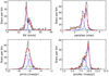 |
Fig. A.1. Best-fit distribution (red lines) of Gamma Vel RVs, parallaxes and proper motions (black histograms), projected onto the four parameters planes. The blue lines show the two cluster components, and the green lines represent the field contribution. |
Appendix B: Properties of selected members
Tables B.1–B.6 (available at the CDS) include the properties of the high-probability members selected for our analysis. Here we show a portion of Table B.1 for 25 Ori as an example.
First and last five lines of the list of high-probability members of 25 Ori.
All Tables
Maximum likelihood best-fit parameters of the RV and astrometry distributions of the sample clusters.
All Figures
|
Fig. 1. Member selection in the γ vs Teff plane for the five clusters in our sample. The magenta lines indicate the exclusion region we adopted for the selection. Stars marked with green diamonds have been excluded as contaminants. |
| In the text | |
|
Fig. 2. GES RV versus parallax (top panels) and proper motion diagrams (bottom panels) for the GES samples for the five clusters after the gravity selection (black dots). In the proper motion diagrams we also plot the density map of the full Gaia samples on a grey scale. The final samples of selected GES and Gaia members are overplotted as red and light red dots, respectively, for 25 Ori, Gamma Vel A, NGC 2451 B, NGC 2547 and NGC 2516, and as blue and light blue dots, respectively, for Gamma Vel B. |
| In the text | |
|
Fig. 3. CMDs (left panels) and lithium distribution as a function of Teff (right panels) of the final samples of selected members for each cluster. The GES and Gaia members are indicated by black and blue dots, respectively. Left panels: only stars with good photometry are plotted. The errors on photometry are smaller than the symbol size. Downward triangles in the lithium diagrams indicate upper limits. |
| In the text | |
|
Fig. 4. Effect of adopting different values of αML and of different spot coverage fractions on the models at 15 Myr (left panels), 30 Myr (middle panels), and 100 Myr (right panels). The top row shows the effect on the CMD, and the bottom row presents the effect on the surface lithium abundance as a function of Teff. The standard reference model with αML = 2 and no spots is plotted as the solid black line. The dashed red and dot-dashed blue lines show the models without spots and αML = 1.5 and 1.0, respectively. The models with αML = 2 and βspot = 0.2 and 0.4 are indicated with the dotted green and three-dot-dashed orange lines, respectively. |
| In the text | |
|
Fig. 5. Comparison of the data with the best-fit model in the CMD (left panels) and in the lithium–Teff plane (right panels) for Gamma Vel A (top) and Gamma Vel B (bottom). Errors on photometry are smaller than the symbol size. Open downward triangles in the lithium diagrams represent upper limits for A(Li). The best-fit model with αML = 1.0 and βspot = 0.2 is shown as a solid blue line, and the isochrones corresponding to the maximum and minimum age derived by the fitting method are shown as dashed and dot-dashed red lines, respectively. The long-dashed green line is the isochrone at the same age, reddening, and αML as the best-fit model, but with βspot = 0. |
| In the text | |
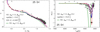 |
Fig. 6. Same as Fig. 5, but for the 25 Ori cluster. |
| In the text | |
|
Fig. 7. Same as Fig. 5 for NGC 2451 B (top) and NGC 2547 (bottom). In this case, the best-fit model (solid blue line) corresponds to αML = 2.0 and βspot = 0. The long-dashed green line shows the isochrone with the same age, reddening, and αML as the best-fit model, but computed with βspot = 0.2. |
| In the text | |
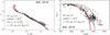 |
Fig. 8. Same as Fig. 7, but for the NGC 2516 cluster. |
| In the text | |
|
Fig. 9. Lithium as a function of the chromospheric activity indicator log LHα/Lbol for detections only (top three panels). First panel: A(Li) for stars with 3000 < Teff < 3700 K in Gamma Vel A (open black circles), Gamma Vel B (open blue squares) and 25 Ori (red stars). Second and third panels: lithium excess ΔA(Li) (see text) for stars with 3000 < Teff < 6000 K in NGC 2451 B and NGC 2547 (second panel, open circles and squares, respectively), and NGC 2516 (third panel, open circles). The red symbols mark stars for which the models predict full lithium depletion. Bottom panel: ΔA(Li) for NGC 2516 members as a function of the Rossby number Ro from Fritzewski et al. (2020). The symbols are the same as in the third panel. |
| In the text | |
|
Fig. A.1. Best-fit distribution (red lines) of Gamma Vel RVs, parallaxes and proper motions (black histograms), projected onto the four parameters planes. The blue lines show the two cluster components, and the green lines represent the field contribution. |
| In the text | |
Current usage metrics show cumulative count of Article Views (full-text article views including HTML views, PDF and ePub downloads, according to the available data) and Abstracts Views on Vision4Press platform.
Data correspond to usage on the plateform after 2015. The current usage metrics is available 48-96 hours after online publication and is updated daily on week days.
Initial download of the metrics may take a while.