| Issue |
A&A
Volume 659, March 2022
|
|
|---|---|---|
| Article Number | A119 | |
| Number of page(s) | 12 | |
| Section | Extragalactic astronomy | |
| DOI | https://doi.org/10.1051/0004-6361/202142212 | |
| Published online | 16 March 2022 | |
Multiple stellar populations in Schwarzschild modeling and the application to the Fornax dwarf
Nicolaus Copernicus Astronomical Center, Polish Academy of Sciences, Bartycka 18, 00-716 Warsaw, Poland
e-mail: This email address is being protected from spambots. You need JavaScript enabled to view it.
, This email address is being protected from spambots. You need JavaScript enabled to view it.
Received:
13
September
2021
Accepted:
27
December
2021
Abstract
Dwarf spheroidal (dSph) galaxies are believed to be strongly dark matter dominated and thus are considered perfect objects to study dark matter distribution and test theories of structure formation. They possess resolved, multiple stellar populations that offer new possibilities for modeling. A promising tool for the dynamical modeling of these objects is the Schwarzschild orbit superposition method. In this work we extend our previous implementation of the scheme to include more than one population of stars and a more general form of the mass-to-light ratio function. We tested the improved approach on a nearly spherical, gas-free galaxy formed in the cosmological context from the Illustris simulation. We modeled the binned velocity moments for stars split into two populations by metallicity and demonstrate that in spite of larger sampling errors the increased number of constraints leads to significantly tighter confidence regions on the recovered density and velocity anisotropy profiles. We then applied the method to the Fornax dSph galaxy with stars similarly divided into two populations. In comparison with our earlier work, we find the anisotropy parameter to be slightly increasing, rather than decreasing, with radius and more strongly constrained. We are also able to infer anisotropy for each stellar population separately and find them to be significantly different.
Key words: galaxies: kinematics and dynamics / galaxies: structure / galaxies: fundamental parameters / galaxies: dwarf / galaxies: star clusters: individual: Fornax
© ESO 2022
1. Introduction
Dwarf spheroidal (dSph) galaxies of the Local Group (Mateo 1998; Tolstoy et al. 2009) are considered to be a perfect tool to test our current theories of structure formation involving dark matter in the context of near-field cosmology. The objects are believed to be strongly dark matter dominated with mass-to-light ratios even on the order of a few hundred solar units. Due to their proximity they are also the only extragalactic systems where individual stars can be resolved and their velocities measured offering the possibility to create interesting dynamical modeling techniques.
The first estimates of dark matter content in dSph galaxies were based on a single measurement of the line-of-sight velocity dispersion of the stars and the application of the virial theorem. As the samples of the stars with kinematic measurements grew, it became possible to estimate the profile of the velocity dispersion and model it using the Jeans equation (Binney & Tremaine 2008). Since the stars in the galaxy can move on a variety of orbits, from circular to radial, the degeneracy between the anisotropy of the orbits and the mass distribution is inherent in this type of modeling. The reason for this lies in the fact that different combinations of these quantities can reproduce the velocity dispersion profile equally well.
A way to overcome this issue, at least partially, is to resort to higher order line-of-sight velocity moments, such as the kurtosis, and use the corresponding Jeans equations. Since the kurtosis is more sensitive to the velocity anisotropy than to the mass distribution, useful constraints can be obtained on both. Still, the method requires large kinematic samples to estimate the velocity moments reliably and some assumption on the functional form of the anisotropy (Łokas 2002; Łokas et al. 2005).
The Schwarzschild modeling technique (Schwarzschild 1979) offers a different approach to estimate the properties of dSph galaxies without prior assumptions on the type of orbits. It relies on building a galaxy model out of a set of best-fitting orbits probed in the range of energy and angular momenta. In this method, the anisotropy of the stellar orbits comes out as a result of the modeling in the same way as the density profile. Although it has been originally developed for large elliptical galaxies (van der Marel et al. 1998; Valluri et al. 2004; Gebhardt et al. 2003), it has recently been adopted for use on discrete data characteristic of dSph galaxies and applied to a number of dwarfs, including Carina, Draco, Fornax, Sculptor, and Sextans (Jardel & Gebhardt 2012; Jardel et al. 2013; Breddels & Helmi 2013; Breddels et al. 2013; Kowalczyk et al. 2019).
Many dSph galaxies show signs of the presence of multiple stellar populations resulting from a few star formation episodes (Bellazzini et al. 2001; del Pino et al. 2015; Fabrizio et al. 2016; Pace et al. 2020). This observation offers a way to improve the modeling methods since, assuming dynamical equilibrium, all populations are supposed to be influenced by the same underlying gravitational potential of the galaxy, but they have different distributions so more constraints can be imposed during the modeling. This approach was first used by Battaglia et al. (2008) to model the mass distribution in the Sculptor dSph galaxy. A few attempts have also been made to constrain the inner slope of the dark matter profile in dSph galaxies using this technique (Walker & Peñarrubia 2011; Amorisco & Evans 2012; Hayashi et al. 2018) in order to resolve the so-called cusp-core problem. It has been shown to be difficult, however, due to the nonsphericity of the dwarfs that introduces biases in such measurements (Kowalczyk et al. 2013; Genina et al. 2018).
In our recent papers (Kowalczyk et al. 2017, 2018, 2019) we developed the Schwarzschild technique in the form applicable to binned velocity moments of a single tracer and verified its ability to reproduce the mass distribution and velocity anisotropy of simulated galaxies. We have also studied biases resulting from the nonsphericity of the modeled objects. Later, we applied the method to model the kinematics of the Fornax dSph galaxy estimating its mass and anisotropy profiles with unprecedented precision.
In this paper we extend our Schwarzschild modeling technique to include multiple stellar populations with the aim to constrain the properties of dSph galaxies even more strongly. We test our approach on a realistic simulated galaxy formed in the cosmological context, originating from the Illustris project (Vogelsberger et al. 2014a). Although no precise analogues of dSph galaxies are available in this simulation because of the resolution, we use a more massive galaxy but with properties otherwise similar to dSphs. The reliability of the modeling does not depend on the particular value of the mass so we believe these tests to be viable. We do not attempt to constrain the inner dark matter density profile (which is poorly resolved anyway) but try to put tighter limits on the estimates of the mass and anisotropy profiles. Finally, we apply the improved method to the available kinematic data for the distinct stellar populations of the Fornax dSph.
This paper is organized as follows. In Sect. 2 we present the data for the simulated galaxy as well as their splitting into stellar populations and mock observations along the main axes. Section 3 contains an overview of our modeling method, the application of the method to all stars and to two populations, and a comparison of the results obtained with these two approaches. The results of the application of the method to the Fornax dSph galaxy are presented in Sect. 4. We discuss our findings and summarize the paper in Sect. 5.
2. Mock data
2.1. Selection of the simulated galaxy
In order to test our modeling method on realistic simulated data, we decided to use a galaxy from the Illustris project (Vogelsberger et al. 2014a,b; Genel et al. 2014; Nelson et al. 2015), namely the Illustris-1 cosmological simulation. This simulation follows the formation and evolution of galaxies from the early Universe to the present by solving gravity and hydrodynamics, as well as modeling of star formation, galactic winds, magnetic fields, and the feedback from black holes. Although dwarf galaxies that are of our interest here are not resolved in the suite, this can be easily overcome with the appropriate choice of the object and the treatment of data.
As the key properties of dSph galaxy equivalents we identified: the lack of gas, the lack of a black hole, a low spin, the stellar mass much smaller than the dark matter mass and a nearly spherical shape. The last condition was adopted in an attempt to avoid any strong bias introduced by the spherical modeling of a nonspherical object. Moreover, we required the galaxy to possess a significant number of both stellar and dark matter particles (over 105), and a well resolved center. Due to the large softening scale for dark matter particles in the simulation (ϵDM = 1.42 kpc), we looked for an object in which even the more concentrated stellar population (see Sect. 2.2) extended over 43 kpc so that the region affected by the numerical artifacts was enclosed within 2−3 innermost data bins (we used 20 linearly spaced spatial bins, see Sect. 3.1).
Out of 27 345 galaxies listed in the catalog of stellar circularities, angular momenta, and axis ratios published by the Illustris team (Genel et al. 2015) containing subhalos with the stellar mass larger than 109 M⊙, only a few met our restrictive requirements. We decided to use a galaxy labeled as subhalo 16 960. All the relevant properties of the galaxy are given in Table 1, including numbers of particles and total masses for both components, and details on the shape of the stellar component: the axis ratios minor to major (shortest to longest) c/a, intermediate to major b/a, and the triaxiality parameter T = (a2 − b2)/(a2 − c2). We distinguish between the half-mass radius provided in the Illustris database and the half-number radius r1/2, which we use for further calculations in this paper. The difference between the two comes from a small gradient in the stellar mass-to-light ratio with the distance from the galactic center. Since in our approach we treat stars as equal-mass particles and refer to number densities (multiplied by the mean mass of a stellar particle when needed), the application of the half-number radius is more self-consistent.
Properties of the Illustris galaxy used to create mock data.
2.2. Splitting the stars into populations
Our chosen galaxy shows a complex formation history undergoing multiple mergers which result in extended star formation with a few star formation bursts. The last wet merger, that is a merger with an object containing gas, happens at 6.9 Gyr from the beginning of the simulation, whereas the last dry merger (no gas transfer) at 12.1 Gyr, giving the galaxy enough time to regain dynamical equilibrium. We present the star formation rate (SFR) as a function of time (the age of the Universe) in Fig. 1, where these last mergers are indicated with black and gray vertical arrows. In Fig. 2 we show the distribution of stars as a function of their metallicity (in solar units) and the time of formation. In order to divide the stellar sample into two populations we cut it in half based on the metallicity index of each stellar particle. This split is indicated in Fig. 2 with the vertical line. With satisfying accuracy it separates the stars born before and after 4 Gyr since the start of the simulation, which corresponds to the formation time before and after the end of the second major star burst, as shown in Fig. 1. We refer to the metal-rich stars as population I and to the metal-poor as population II, following the commonly used nomenclature in astronomy.
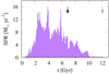 |
Fig. 1. Star formation rate as a function of the age of the Universe in the simulated galaxy from the Illustris project used to create mock data. The black and gray vertical arrows indicate the last mergers which the galaxy underwent, wet and dry, respectively. |
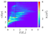 |
Fig. 2. Number of stars as a function of their metallicity and time of formation (the age of the Universe) in the simulated galaxy. The vertical line indicates the applied split into stellar populations. |
In Fig. 3 we present maps of the projected stellar mass density, line-of-sight velocity, and line-of-sight velocity dispersion for both populations obtained by projecting the galaxy along its principal axes. The orientation was determined from the inertia tensor calculated from all stars within the half-number radius r1/2 and therefore is the same in both panels. The two populations differ significantly in the spatial distribution and kinematics with the metal-rich (considered to be younger) population I being more concentrated but having lower central velocity dispersion. Both populations show a weak rotation signal at large distances from the center.
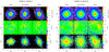 |
Fig. 3. Maps of the projected stellar density, mean stellar velocity, and stellar velocity dispersion (in rows) for two stellar populations: the metal-rich population I (left-hand side panels) and the metal-poor population II (right-hand side), and observations along the principal axes determined for all stars (in columns, along the major, the intermediate, and the minor axis, respectively). |
The velocity anisotropy parameter  , where σi are velocity dispersions in spherical coordinates (Binney & Tremaine 2008), describes the orbital structure of galaxies. It is one of the most important dynamical properties of bound systems which cannot be inferred directly from observations and has to be recovered by dynamical modeling. The profiles of the anisotropy parameter β as well as the radial σr and tangential
 ![Mathematical equation: $ \sigma_t = [(\sigma_\theta^2 + \sigma_\phi^2)/2]^{1/2} $](/articles/aa/full_html/2022/03/aa42212-21/aa42212-21-eq2.gif) velocity dispersions for our simulated galaxy are presented in the consecutive columns of Fig. 4. Throughout the paper we use red, orange, and blue colors to indicate values calculated or recovered for all stars, population I, and population II, respectively. The two rows of the figure show the behavior of the parameters at different scales. The top row plots the profiles with the distance from the center of the galaxy in the logarithmic scale and shows the drop of anisotropy at the outer edges of the object. The bottom row uses the linear distance scale and focuses on the main body of the galaxy.
velocity dispersions for our simulated galaxy are presented in the consecutive columns of Fig. 4. Throughout the paper we use red, orange, and blue colors to indicate values calculated or recovered for all stars, population I, and population II, respectively. The two rows of the figure show the behavior of the parameters at different scales. The top row plots the profiles with the distance from the center of the galaxy in the logarithmic scale and shows the drop of anisotropy at the outer edges of the object. The bottom row uses the linear distance scale and focuses on the main body of the galaxy.
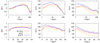 |
Fig. 4. Profiles of the velocity anisotropy parameter, radial velocity dispersion, and tangential velocity dispersion (in consecutive columns) calculated from all stars (in red), including only population I (in orange), and only population II (in blue). Upper row: profiles using the logarithmic distance scale and reaching the outskirts of the galaxy; bottom row: the radial range used in the modeling shown in the linear scale. |
Figure 5 shows the surface number density profiles of the stars as measured in different directions. We can see that while the different subsamples have quite distinguishable profiles, the difference between the lines of sight is small because the galaxy is close to spherical.
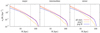 |
Fig. 5. Surface number density profiles of the stellar data samples for the simulated galaxy observed along different lines of sight (from the left to the right). Different lines show profiles for all available stars (in red), the metal-rich population I (in orange), and the metal-poor population II (in blue). Thin vertical lines indicate r0 (see text) and the outer boundary of the spectroscopic data. |
2.3. Observables
We generated nine sets of mock data by observing all stars and each population separately along the principal axes determined from all stars. For the observables to be used in the modeling we divided the stars into 20 bins spaced linearly in distance from the center of the galaxy up to 50 kpc, measuring the fraction of the total number of stars and the 2nd, 3rd, and 4th proper moments of the line-of-sight velocity defined in Eqs. (8) and (9) of Kowalczyk et al. (2018). The profiles of these quantities are shown in consecutive rows in Fig. 6. Columns correspond to different lines of sight, from the left to the right: along the major, intermediate, and minor axis of the galaxy. For clarity of the figure, in each panel we indicate only the error bars for one of the data sets. However, as the number of stars in a sample remains roughly constant between the lines of sight, the error bars are very similar among the panels in a given row.
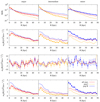 |
Fig. 6. Observables used in our Schwarzschild modeling scheme of the simulated galaxy. In rows: the fraction of the total number of stars, 2nd, 3rd, and 4th velocity moment. In columns: mock data from the simulated galaxy along the major, intermediate, and minor axis. In red we present the values obtained for all stars whereas in orange and blue those for populations I and II, respectively. For clarity of the figure, in each panel we indicate only the error bars for one of the data sets. |
Although in our previous studies of the reliability of the Schwarzschild modeling and its applications to real data (Kowalczyk et al. 2017, 2018, 2019) we approximated the density profile of the tracer with the Sérsic formula, we found that it does not provide a good approximation of the data for the simulated galaxy considered here. We therefore fit the projected density profile with the King formula (King 1962)
![Mathematical equation: $$ \begin{aligned} I(R) = I_0 \left[\frac{1}{\sqrt{1+(R/R_{\rm c})^2}}-\frac{1}{\sqrt{1+(R_{\rm t}/R_{\rm c})^2}}\right]^2, \end{aligned} $$](/articles/aa/full_html/2022/03/aa42212-21/aa42212-21-eq3.gif) (1)
(1)
where I0, Rc, and Rt are the model parameters. The profile can be analytically deprojected to obtain the 3D density
![Mathematical equation: $$ \begin{aligned} \rho (r) = \frac{\rho _0}{z^2} \left[\frac{1}{z}\arccos (z)-\sqrt{1-z^2}\right], \end{aligned} $$](/articles/aa/full_html/2022/03/aa42212-21/aa42212-21-eq4.gif) (2)
(2)
where
![Mathematical equation: $$ \begin{aligned} \rho _0 = \frac{I_0}{\pi R_{\rm c} [1+(R_{\rm t}/R_{\rm c})^2]^{3/2}} \end{aligned} $$](/articles/aa/full_html/2022/03/aa42212-21/aa42212-21-eq5.gif) (3)
(3)
and
 (4)
(4)
3. Schwarzschild modeling
In this section we briefly present our modeling method and its application to the data sets derived for all stars and the two populations of the simulated galaxy separately. In both cases our aim was to recover the profiles of the total mass and the velocity anisotropy.
3.1. Overview of the method
We follow the approach introduced in Kowalczyk et al. (2018), namely we model the total mass profile with the mass-to-light ratio Υ varying with radius:
 (5)
(5)
where r is the distance from the center of the galaxy, r0 is a constant, while Υ0, a, and c are the parameters of a model. We have assumed log r0 = 0.33 which corresponds to three softening scales for stellar particles in the Illustris simulation.
We probed the parameter a ∈ [0 : 1.3] with a step Δa = 0.04 and c ∈ [1.1 : 2.9] with a step Δc = 0.2, imposing the requirement on the total density profile to be monotonically decreasing with radius. For each set of parameters and for each line of sight we generated 1200 orbits using 100 values of energy (expressed with the radius of a circular orbit) spaced logarithmically and 12 values of the relative angular momentum spaced linearly. The outer radius of the orbit library, that is the apocenter of the most extended orbit, was set to rout = 165 kpc in order to cover over 0.999 of the total stellar mass based on the fitted King profile parameters.
We fit the kinematics weighted with the fraction of mass with the constrained least squares algorithm where different values of Υ0 were obtained with a simple transformation of velocities given by Eqs. (12), (13), and (15) in Kowalczyk et al. (2018). In order to smooth out the numerical artifacts, the three-dimensional χ2 spaces were then interpolated with 12-order polynomials ( ) that were further used to determine the global minimums (identified as the best-fitting models) and 1, 2, 3σ confidence levels which for three parameters correspond to Δχ2 = 3.53, 8.02, 14.2 (Press et al. 1992).
3.2. Application to mock data
In the following we present the direct and inferred results of the Schwarzschild modeling of the data sets described in Sect. 2.3.
First, Fig. 7 shows the distribution of the absolute values of the χ2 as a function of three parameters of the mass-to-light ratio. In order to avoid unnecessary repetitions, we include only the plot for the mock data obtained by observing the Illustris galaxy along its major axis as the others are qualitatively similar. The four panels refer to fits for all stars (top left), the metal-rich population I (bottom left), the metal-poor population II (bottom right), and the one named “populations” (top right) which is the algebraic sum of values for both populations.
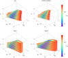 |
Fig. 7. Absolute values of χ2 obtained from the fits of three data sets: all stars (top left panel), population I (bottom left), and population II (bottom right) for the observations along the major axis of the simulated galaxy. The results for the modeling of two populations (top right) were obtained as an algebraic sum of values for populations I and II. To avoid large numbers in the figure, Υ0 was divided by the mean mass of a stellar particle. |
As our parametrization of the mass-to-light ratio is not intuitive we present its profiles explicitly in the first rows of the left- and right-hand side panels of Fig. 8 for the results obtained for all stars and the populations, respectively. We further calculate the total density (second rows) and the total mass content (third rows). We include the obtained orbit anisotropy within the modeled range in the bottom rows. The consecutive columns present the results for the observations along the major, intermediate, and minor axis. Green lines indicate values for the best-fit models whereas the colored areas of decreasing intensity correspond to 1, 2, and 3σ confidence regions obtained as extreme values allowed by the models with χ2 within a given region. In each panel the true values from the simulation are presented with black lines while thin vertical lines mark the values of r0 and the outer range of the data sets beyond which the reliability of results drops significantly. The true mass-to-light ratio profile was obtained by dividing the total mass by the fitted King profiles, therefore the drop at 100 kpc is the numerical artifact occurring at the very outskirts of the galaxy.
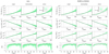 |
Fig. 8. Left-hand side: results of Schwarzschild modeling of three mock data sets obtained by observing the simulated galaxy along the principal axes. In rows: derived mass-to-light ratio, total density, total mass, and anisotropy parameter. In columns: observations along the major, intermediate, and minor axis, respectively. Green lines indicate values for the best-fit models whereas the colored areas of decreasing intensity show the 1, 2, and 3σ confidence levels. The true values are presented as black lines. Thin vertical lines mark the values of r0 and the outer range of the data sets, from left to right. Right-hand side: same as left but for the fit of two stellar populations. |
Whereas in the right-hand side panels of Fig. 8 the resulting anisotropy is obtained from the fit of all stars and uses only the location of global minimum and confidence levels from two populations (as in the top right panel of Fig. 7), in Fig. 9 we present another method of calculating the anisotropy. In the second and third row we show the derived profiles for population I and II separately and combine them as stellar mass weighted average in the top row. As in previous figures, three columns refer to the different lines of sight whereas the narrow fourth one shows the behavior of the true profiles outside the modeled range which, as we noticed in our previous studies, in a limited way influences the results. Such an impact is understandable since the stars at larger distances from the center are still included in the line-of-sight measurements.
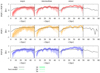 |
Fig. 9. Profiles of the anisotropy parameter obtained with the Schwarzschild modeling of two stellar populations of the simulated galaxy. In rows: results for all stars (calculated as the superposition of two populations), population I, and population II. Colors follow the convention used in previous figures. In columns: observations along the major, intermediate, and minor axis. The last narrower column shows the data (black lines) outside the modeled radial range. Color lines indicate values for the best-fit models whereas the colored areas of decreasing intensity show the 1, 2, and 3σ confidence regions. |
3.3. Comparison of fitting results
The main strength of the two populations method comes from tracing the underlying gravitational potential at different scales. As can be seen in the bottom panels of Fig. 7, population I, which is more concentrated, is also more sensitive to Υ0, but gives weaker constraints on a or c. On the other hand, population II attempts to reproduce the total mass content at larger distances as well, therefore showing stronger coupling between the parameters.
The global minimums of the χ2 distributions for both approaches, that is modeling one and two populations, which we identify as the best-fitting models, closely coincide showing that there is no internal bias in the improved method. However, significant differences can be observed when comparing the confidence levels, mainly at 1 and 3σ. Namely, we find that using two populations, the constraints we obtain on the density and anisotropy profile are much stronger.
Additionally, the more accurate method allows us to study other effects and biases, for example the consequences of the nonsphericity of the modeled object. Whereas for the fit of all stars the true values of the density, mass, and anisotropy profiles are contained within 1σ confidence regions, the results for the populations are more or less biased depending on the axis. They are well reproduced for the observation along the intermediate axis, for which the effects of nonsphericity seem to cancel out, and more biased for the remaining lines of sight. We notice a trend from under- to overestimation of the anisotropy when going from the major to the minor axis.
4. Modeling Fornax dSph
In this section we present the application of our Schwarzschild modeling scheme to the observational data for the Fornax dSph galaxy obtained by del Pino et al. (2015, 2017). This study is a follow-up of the work of Kowalczyk et al. (2019) and can be directly compared to the results presented there. Moreover, we refer the reader to these previous publications for details on the origin of data and our procedures used for cleaning the spectroscopic sample.
Similarly to the approach introduced in Sect. 2.2, we divided all available stars into two equal-size populations based on their metallicity and then cross-correlated the samples with the data used in Kowalczyk et al. (2019). The metallicity histogram of the final spectroscopic sample is shown in Fig. 10. Additionally, we color-coded each bin with the population it has been assigned to, namely orange or blue for population I or II. Interestingly, the case of Fornax is similar to our simulated galaxy as the split at [Fe/H] = −1 also captures an important feature of the object’s star formation history, separating stars into subsamples older and younger than 6 Gyr, as shown in Fig. 12 of del Pino et al. (2015) and Fig. 8 of del Pino et al. (2017). The numbers of stars contained in the samples of all stars, population I, and population II are given in Table 2, where the indices “phot” and “spec” refer to the photometric and kinematic samples. The sum of stars in the populations is lower than in the sample of all stars since only stars with reliable measurements of metallicity could be included.
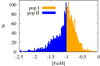 |
Fig. 10. Metallicity histogram of the final spectroscopic sample used in the modeling of two stellar populations in the Fornax dSph. Each bin is color-coded according to the population it has been assigned to, orange or blue for population I and II, respectively. |
Properties of the data samples for the Fornax dSph.
As we have shown in our earlier work, the light profile of the Fornax dSph can be well reproduced with the three-parameter Sérsic formula (Sérsic 1968). The profiles of number density for all stars and both populations together with the best-fitting Sérsic profiles are presented in Fig. 11. The colors follow the convention introduced in previous sections. Thin vertical lines indicate the innermost data point for the light profile for all stars and the outer boundary of the kinematic sample. The former, set at log r = −0.16, is also used as the minimum of the mass-to-light ratio profile (r0 in Eq. (5)). The fitted parameters of the profiles, that is the normalization N0, the Sérsic radius RS, and the Sérsic parameter m, are included in the second part of Table 2.
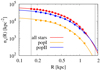 |
Fig. 11. Surface number density profiles of the photometric data samples for the Fornax dSph: all available stars (in red), the metal-rich population I (in orange), and the metal-poor population II (in blue). Thin vertical lines indicate r0 (see text) and the outer boundary of the spectroscopic data. |
Figure 12 presents the profiles of the observables used in the Schwarzschild modeling: the fraction of stars and the 2nd, 3rd, and 4th velocity moments (top to bottom) for the three data samples: all stars, population I, and population II (in red, orange, and blue, respectively). The error bars indicate 1σ sampling errors.
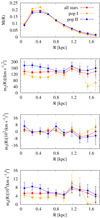 |
Fig. 12. Observables of the Fornax dSph used in our Schwarzschild modeling scheme. In rows: the fraction of the total number of stars, the 2nd, 3rd, and 4th velocity moment. In red we present the values obtained for all stars whereas in orange and blue those for populations I and II, respectively. |
The parameter space for Υ(r) has been probed as follows: a ∈ [0 : 1.85] with a step Δa = 0.05 and c ∈ [1.2 : 6] with a step Δc = 0.2. We point out that in Kowalczyk et al. (2019) the parameter c was fixed at c = 3 and now we fit it as a free parameter. As for the mock data in Sect. 3.2, different values of Υ0 were obtained with the transformation of velocity moments within the χ2 fitting routine. The values of Δχ2 for all stars and the populations are shown in the two panels of Fig. 13 (left and right-hand side, respectively). Due to the dense coverage of the grid, we decided to include only the values within 3σ from the fitted minimums (see Sect. 3.1).
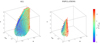 |
Fig. 13. Values of χ2 relative to the fitted minimum within the range of 3σ confidence level for all stars (left panel) and for the populations (right panel) for the Fornax dSph. |
The profiles of the mass-to-light ratio, total density, total mass, and velocity anisotropy resulting from the χ2 distributions are presented in the consecutive rows of Fig. 14. The anisotropy profile for the populations is based on the fit of all stars but using the confidence levels on Υ from the fit of two populations. Green lines indicate the values for the best-fitting models whereas the colored areas of decreasing intensity show the 1, 2, and 3σ confidence regions. Additionally, with black dashed lines we include the results from Kowalczyk et al. (2019) for comparison.
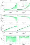 |
Fig. 14. Results of Schwarzschild modeling of the Fornax dSph. In rows: derived mass-to-light ratio, total density, total mass, and anisotropy parameter. In columns: results for all stars and the populations, respectively. Green lines indicate the values for the best-fit models whereas the colored areas of decreasing intensity show the 1, 2, and 3σ confidence regions. The best-fitting values obtained by Kowalczyk et al. (2019) are shown with black dashed lines. |
As a result of freeing the steepness of the mass-to-light ratio profile (parameter c) with respect to the previous study (Kowalczyk et al. 2019), we obtained higher estimates of the enclosed total mass at larger radii. In particular, for the mass enclosed within 1.8 kpc we get  from the fit for all stars and
  from the fit of populations, while previously we had
  .
.
Interestingly, despite the significant shift of the position of  (to c = 4.2 for all stars and 3.6 for populations), the obtained profile of the anisotropy parameter remains decreasing or flat for all stars but changes to increasing from 0 to 0.5 for the populations. Nevertheless, even in the latter case the previous result agrees with the new finding within 1σ.
The detailed analysis of the anisotropy is shown in Fig. 15 where the middle and bottom panels present the profiles obtained for each population separately. We notice that the profile for population I is decreasing or has a local minimum whereas for population II is increasing (from −0.25 to 0.5 for the best-fitting model). Since population I is more concentrated, the last bins contain very few stars, which limits their credibility. The top panel of Fig. 15 presents the anisotropy of all stars calculated as a weighted superposition of two populations. With such approach we still obtain the increasing profile (from 0 to 0.5) but the previous result agrees with it only within 2σ.
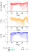 |
Fig. 15. Profiles of the anisotropy parameter obtained with the Schwarzschild modeling of two stellar populations for the Fornax dSph. In rows: results for all stars (calculated as the superposition of two populations), population I, and population II. Color lines indicate values for the best-fit models whereas the colored areas of decreasing intensity show the 1, 2, and 3σ confidence regions. The dashed black line shows the result from Kowalczyk et al. (2019) for comparison. |
Since Fornax dSph is significantly elongated with the projected ellipticity of ϵ = 0.30 ± 0.01 (Irwin & Hatzidimitriou 1995), we anticipate some bias in the obtained results caused by the spherically symmetric modeling. Kowalczyk et al. (2018) studied such bias in an axisymmetric simulated object qualitatively similar to Fornax and identified differences in the systematic errors depending on whether the galaxy was observed along its major or minor axis. Assuming that Fornax is observed along the line of sight in between these extremes, we expect the total mass profile to be slightly overestimated and the anisotropy to be underestimated, further strengthening the likelihood of the real anisotropy to be radial and its profile to be growing with radius with respect to the results of Kowalczyk et al. (2019).
Both constant (like for our population I) and growing (population II) anisotropy profiles can arise from biased modeling of the real growing profile by observing an object along the minor and major axis, respectively. However, for the bias to occur in two populations presented here, their inner orientations would need to be opposite. Since such morphological features are not supported by the photometric studies of Fornax (del Pino et al. 2015; Wang et al. 2019) which rather find a good spatial alignment between the stellar populations, we conclude that the anisotropy profiles of the two populations modeled in this work are indeed significantly distinct.
Finally, it is worth noticing that the so-called mass-follows-light model, that is the one following from the assumption that the total density traces the stellar distribution, is no longer supported by the fit of the populations. With our parametrization, the mass-follows-light model corresponds to a = 0 and whereas it is enclosed within 3σ for the fit of all stars, as was the case in Kowalczyk et al. (2019), the allowed values for the improved method are much larger, as demonstrated by the right panel of Fig. 13.
5. Summary and discussion
Building on the previously created implementation of the Schwarzschild orbit superposition method focused on modeling dSph galaxies of the Local Group (Kowalczyk et al. 2017, 2018, 2019), we improved our tool by introducing multiple stellar populations. Such an improvement is desirable and justified since many of the dwarfs show signs of multiple star formation bursts or extended star formation episodes. As the different populations trace the common underlying gravitational potential, one may expect a significant improvement in the estimates of not only the total mass content but also the orbit anisotropy since this robust modeling technique reproduces the anisotropy as a by-product of the modeling rather than taking it as an assumption.
We have tested our hypothesis by modeling mock data generated from a galaxy formed in the Illustris simulation. Due to the limitations of the resolution, we chose a galaxy of mass a few orders of magnitude larger than the estimated masses of classical dwarfs. Still, the galaxy possessed appropriate qualitative characteristics, such as the lack of gas and an almost spherical shape, that made it a good test bed for modeling techniques applicable to dSph galaxies. We applied our approach to all data and to two stellar populations separately, comparing the accuracy of the obtained results. Although the addition of the second tracer seemingly increases the number of constraints twice, the increment is somewhat compromised by the sampling errors since the number of stars in each sample is then reduced. Still, we found strong improvements in the accuracy of the method when using two populations. The results of the modeling show that the density and velocity anisotropy profiles are more strongly constrained, most importantly at the 3σ level, that is the range of allowed values is much narrower.
Similarly to the conclusions of Kowalczyk et al. (2018) who explored the effects of nonsphericity using large and small data samples, the comparison of results presented in the left- and right-hand side panels of Fig. 8 suggests that the improved method using two stellar populations gives more precise but less accurate outcome. However, in both studies the apparent deterioration of the reliability is a consequence of modeling of a nonspherical object. In both cases, a simpler approach (much smaller data samples or using one stellar population) resulted in larger final uncertainties, usually containing the true values within 1σ confidence region. On the other hand, the improved methods exhibit substantially reduced uncertainties, highlighting the underlying bias.
Our method parametrizes the total mass content with the mass-to-light ratio varying with radius as a power-law in the log-log scale. We made two main changes with respect to our previous work: we added a third parameter c controlling the steepness of the mass-to-light ratio profile (previously fixed at the value of 3) and allowed for different stellar density profiles (previously only Sérsic, now also King). These changes are of course coupled since different density profiles require different exponents to reproduce the same mass profile. It is visible also in our results since the King profile applied in the simulated galaxy gave us values of c lower than 3. Nevertheless, we decided to use different density profiles to make our method more general and applicable to objects, such as our Illustris galaxy, for which the Sérsic formula does not provide a good approximation of the density distribution.
Finally, we applied the improved method to the data for the Fornax dSph galaxy. Due to the addition of another free parameter in our functional form for the mass-to-light ratio, our results for modeling all stars are slightly different from the ones obtained in Kowalczyk et al. (2019). However, in terms of the total density and mass distribution the estimates obtained here agree very well with those earlier results in the range covered by the data. Therefore, the detailed comparison with other estimates from the literature presented in Kowalczyk et al. (2019) is still valid and we do not repeat it here.
A more significant difference with respect to these previous estimates is seen in the results of modeling two populations in Fornax. In this case we find the anisotropy to be slightly increasing rather than decreasing with radius and, most importantly, the confidence regions for this parameter, as well as for the density, are much narrower. We were thus able to obtain tighter constraints on the properties of Fornax, which means that the improved method is successful. For the first time, we were also able to deduce the velocity anisotropy profiles for each of the populations separately. We found that the more concentrated, metal-rich population I has a decreasing anisotropy profile while the more extended, metal-poor population II has the anisotropy increasing with radius. This finding may partially explain the large spread of the anisotropy values obtained in the literature and summarized in Tables 2 and 3 of Kowalczyk et al. (2019), which were often based on modeling subsamples of our spectroscopic data set.
For both studied objects we split the stars into two populations by dividing them in half based on their metallicity, Z (in solar units), for the Illustris galaxy and [Fe/H] for Fornax. Such a method is approximate but justified. Both galaxies have complex star formation history with multiple star formation bursts, as demonstrated by Fig. 1 in this work and Fig. 7 in del Pino et al. (2013), producing multiple stellar populations which cannot be easily tracked as the metallicity is a good but not perfect proxy for the stellar age. Moreover, the metallicity histograms for both objects are approximately unimodal not allowing for a convenient separation. More refined methods of division have been suggested in the literature, for example in the form of the likelihood function based on the position, velocity, and metallicity index (Walker & Peñarrubia 2011). However, the likelihood function requires many assumptions which introduce additional uncertainties into the treatment of the data. On the other hand, our approach ensures the maximization of each sample (and therefore minimization of sampling errors) while capturing the important features of the star formation history.
Further improvements to the Schwarzschild modeling method are certainly possible. One way to proceed would be to include the modeling of the proper motions of the stars. For now, measurements of transverse velocities are available only for the brightest stars in dSph galaxies, but even small samples of this type could provide further constraints on the models, as demonstrated by Strigari et al. (2007) and Massari et al. (2020).
Acknowledgments
We are grateful to Andrés del Pino for providing the data for the Fornax dSph and to the Illustris team for making their simulations publicly available. Useful comments from the anonymous referee are kindly appreciated. This research was supported by the Polish National Science Center under grant 2018/28/C/ST9/00529.
References
- Amorisco, N. C., & Evans, N. W. 2012, MNRAS, 419, 184 [NASA ADS] [CrossRef] [Google Scholar]
- Battaglia, G., Helmi, A., Tolstoy, E., et al. 2008, ApJ, 681, L13 [NASA ADS] [CrossRef] [Google Scholar]
- Bellazzini, M., Ferraro, F. R., & Pancino, E. 2001, MNRAS, 327, L15 [NASA ADS] [CrossRef] [Google Scholar]
- Binney, J., & Tremaine, S. 2008, Galactic Dynamics, 2nd edn. (Princeton: Princeton University Press) [Google Scholar]
- Breddels, M. A., & Helmi, A. 2013, A&A, 558, A35 [NASA ADS] [CrossRef] [EDP Sciences] [Google Scholar]
- Breddels, M. A., Helmi, A., van den Bosch, R. C. E., van de Ven, G., & Battaglia, G. 2013, MNRAS, 433, 3173 [NASA ADS] [CrossRef] [Google Scholar]
- del Pino, A., Hidalgo, S. L., Aparicio, A., et al. 2013, MNRAS, 433, 1505 [Google Scholar]
- del Pino, A., Aparicio, A., & Hidalgo, S. L. 2015, MNRAS, 454, 3996 [NASA ADS] [CrossRef] [Google Scholar]
- del Pino, A., Aparicio, A., Hidalgo, S. L., & Łokas, E. L. 2017, MNRAS, 465, 3708 [NASA ADS] [CrossRef] [Google Scholar]
- Fabrizio, M., Bono, G., Nonino, M., et al. 2016, ApJ, 830, 126 [NASA ADS] [CrossRef] [Google Scholar]
- Gebhardt, K., Richstone, D., Tremaine, S., et al. 2003, ApJ, 583, 92 [Google Scholar]
- Genel, S., Vogelsberger, M., Springel, V., et al. 2014, MNRAS, 445, 175 [Google Scholar]
- Genel, S., Fall, S. M., Hernquist, L., et al. 2015, ApJ, 804, L40 [NASA ADS] [CrossRef] [Google Scholar]
- Genina, A., Benitez-Llambay, A., Frenk, C. S., et al. 2018, MNRAS, 474, 1398 [NASA ADS] [CrossRef] [Google Scholar]
- Hayashi, K., Fabrizio, M., Łokas, E. L., et al. 2018, MNRAS, 481, 250 [NASA ADS] [CrossRef] [Google Scholar]
- Irwin, M., & Hatzidimitriou, D. 1995, MNRAS, 277, 1354 [NASA ADS] [CrossRef] [Google Scholar]
- Jardel, J. R., & Gebhardt, K. 2012, ApJ, 746, 89 [NASA ADS] [CrossRef] [Google Scholar]
- Jardel, J. R., Gebhardt, K., Fabricius, M. H., Drory, N., & Williams, M. J. 2013, ApJ, 763, 91 [NASA ADS] [CrossRef] [Google Scholar]
- King, I. 1962, AJ, 67, 471 [Google Scholar]
- Kowalczyk, K., Łokas, E. L., Kazantzidis, S., & Mayer, L. 2013, MNRAS, 431, 2796 [NASA ADS] [CrossRef] [Google Scholar]
- Kowalczyk, K., Łokas, E. L., & Valluri, M. 2017, MNRAS, 470, 3959 [NASA ADS] [CrossRef] [Google Scholar]
- Kowalczyk, K., Łokas, E. L., & Valluri, M. 2018, MNRAS, 476, 2918 [NASA ADS] [CrossRef] [Google Scholar]
- Kowalczyk, K., del Pino, A., Łokas, E. L., & Valluri, M. 2019, MNRAS, 482, 5241 [NASA ADS] [CrossRef] [Google Scholar]
- Łokas, E. L. 2002, MNRAS, 333, 697 [CrossRef] [Google Scholar]
- Łokas, E. L., Mamon, G. A., & Prada, F. 2005, MNRAS, 363, 918 [CrossRef] [Google Scholar]
- Massari, D., Helmi, A., Mucciarelli, A., et al. 2020, A&A, 633, A36 [NASA ADS] [CrossRef] [EDP Sciences] [Google Scholar]
- Mateo, M. 1998, ARA&A, 36, 435 [NASA ADS] [CrossRef] [Google Scholar]
- Nelson, D., Pillepich, A., Genel, S., et al. 2015, Astron. Comput., 13, 12 [Google Scholar]
- Pace, A. B., Kaplinghat, M., Kirby, E., et al. 2020, MNRAS, 495, 3022 [NASA ADS] [CrossRef] [Google Scholar]
- Press, W. H., Teukolsky, S. A., Vetterling, W. T., & Flannery, B. P. 1992, Numerical Recipes in C, 2nd edn. (Cambridge: Cambridge University Press) [Google Scholar]
- Schwarzschild, M. 1979, ApJ, 232, 236 [NASA ADS] [CrossRef] [Google Scholar]
- Sérsic, J. L. 1968, Atlas de Galaxias Australes (Cordoba, Argentina: Observatorio Astronomico) [Google Scholar]
- Strigari, L. E., Bullock, J. S., & Kaplinghat, M. 2007, ApJ, 657, L1 [Google Scholar]
- Tolstoy, E., Hill, V., & Tosi, M. 2009, ARA&A, 47, 371 [Google Scholar]
- Valluri, M., Merritt, D., & Emsellem, E. 2004, ApJ, 602, 66 [Google Scholar]
- van der Marel, R. P., Cretton, N., de Zeeuw, P. T., & Rix, H.-W. 1998, ApJ, 493, 613 [Google Scholar]
- Vogelsberger, M., Genel, S., Springel, V., et al. 2014a, Nature, 509, 177 [Google Scholar]
- Vogelsberger, M., Genel, S., Springel, V., et al. 2014b, MNRAS, 444, 1518 [Google Scholar]
- Walker, M. G., & Peñarrubia, J. 2011, ApJ, 742, 20 [CrossRef] [Google Scholar]
- Wang, M. Y., de Boer, T., Pieres, A., et al. 2019, ApJ, 881, 118 [NASA ADS] [CrossRef] [Google Scholar]
All Tables
All Figures
|
Fig. 1. Star formation rate as a function of the age of the Universe in the simulated galaxy from the Illustris project used to create mock data. The black and gray vertical arrows indicate the last mergers which the galaxy underwent, wet and dry, respectively. |
| In the text | |
|
Fig. 2. Number of stars as a function of their metallicity and time of formation (the age of the Universe) in the simulated galaxy. The vertical line indicates the applied split into stellar populations. |
| In the text | |
|
Fig. 3. Maps of the projected stellar density, mean stellar velocity, and stellar velocity dispersion (in rows) for two stellar populations: the metal-rich population I (left-hand side panels) and the metal-poor population II (right-hand side), and observations along the principal axes determined for all stars (in columns, along the major, the intermediate, and the minor axis, respectively). |
| In the text | |
|
Fig. 4. Profiles of the velocity anisotropy parameter, radial velocity dispersion, and tangential velocity dispersion (in consecutive columns) calculated from all stars (in red), including only population I (in orange), and only population II (in blue). Upper row: profiles using the logarithmic distance scale and reaching the outskirts of the galaxy; bottom row: the radial range used in the modeling shown in the linear scale. |
| In the text | |
|
Fig. 5. Surface number density profiles of the stellar data samples for the simulated galaxy observed along different lines of sight (from the left to the right). Different lines show profiles for all available stars (in red), the metal-rich population I (in orange), and the metal-poor population II (in blue). Thin vertical lines indicate r0 (see text) and the outer boundary of the spectroscopic data. |
| In the text | |
|
Fig. 6. Observables used in our Schwarzschild modeling scheme of the simulated galaxy. In rows: the fraction of the total number of stars, 2nd, 3rd, and 4th velocity moment. In columns: mock data from the simulated galaxy along the major, intermediate, and minor axis. In red we present the values obtained for all stars whereas in orange and blue those for populations I and II, respectively. For clarity of the figure, in each panel we indicate only the error bars for one of the data sets. |
| In the text | |
|
Fig. 7. Absolute values of χ2 obtained from the fits of three data sets: all stars (top left panel), population I (bottom left), and population II (bottom right) for the observations along the major axis of the simulated galaxy. The results for the modeling of two populations (top right) were obtained as an algebraic sum of values for populations I and II. To avoid large numbers in the figure, Υ0 was divided by the mean mass of a stellar particle. |
| In the text | |
|
Fig. 8. Left-hand side: results of Schwarzschild modeling of three mock data sets obtained by observing the simulated galaxy along the principal axes. In rows: derived mass-to-light ratio, total density, total mass, and anisotropy parameter. In columns: observations along the major, intermediate, and minor axis, respectively. Green lines indicate values for the best-fit models whereas the colored areas of decreasing intensity show the 1, 2, and 3σ confidence levels. The true values are presented as black lines. Thin vertical lines mark the values of r0 and the outer range of the data sets, from left to right. Right-hand side: same as left but for the fit of two stellar populations. |
| In the text | |
|
Fig. 9. Profiles of the anisotropy parameter obtained with the Schwarzschild modeling of two stellar populations of the simulated galaxy. In rows: results for all stars (calculated as the superposition of two populations), population I, and population II. Colors follow the convention used in previous figures. In columns: observations along the major, intermediate, and minor axis. The last narrower column shows the data (black lines) outside the modeled radial range. Color lines indicate values for the best-fit models whereas the colored areas of decreasing intensity show the 1, 2, and 3σ confidence regions. |
| In the text | |
|
Fig. 10. Metallicity histogram of the final spectroscopic sample used in the modeling of two stellar populations in the Fornax dSph. Each bin is color-coded according to the population it has been assigned to, orange or blue for population I and II, respectively. |
| In the text | |
|
Fig. 11. Surface number density profiles of the photometric data samples for the Fornax dSph: all available stars (in red), the metal-rich population I (in orange), and the metal-poor population II (in blue). Thin vertical lines indicate r0 (see text) and the outer boundary of the spectroscopic data. |
| In the text | |
|
Fig. 12. Observables of the Fornax dSph used in our Schwarzschild modeling scheme. In rows: the fraction of the total number of stars, the 2nd, 3rd, and 4th velocity moment. In red we present the values obtained for all stars whereas in orange and blue those for populations I and II, respectively. |
| In the text | |
|
Fig. 13. Values of χ2 relative to the fitted minimum within the range of 3σ confidence level for all stars (left panel) and for the populations (right panel) for the Fornax dSph. |
| In the text | |
|
Fig. 14. Results of Schwarzschild modeling of the Fornax dSph. In rows: derived mass-to-light ratio, total density, total mass, and anisotropy parameter. In columns: results for all stars and the populations, respectively. Green lines indicate the values for the best-fit models whereas the colored areas of decreasing intensity show the 1, 2, and 3σ confidence regions. The best-fitting values obtained by Kowalczyk et al. (2019) are shown with black dashed lines. |
| In the text | |
|
Fig. 15. Profiles of the anisotropy parameter obtained with the Schwarzschild modeling of two stellar populations for the Fornax dSph. In rows: results for all stars (calculated as the superposition of two populations), population I, and population II. Color lines indicate values for the best-fit models whereas the colored areas of decreasing intensity show the 1, 2, and 3σ confidence regions. The dashed black line shows the result from Kowalczyk et al. (2019) for comparison. |
| In the text | |
Current usage metrics show cumulative count of Article Views (full-text article views including HTML views, PDF and ePub downloads, according to the available data) and Abstracts Views on Vision4Press platform.
Data correspond to usage on the plateform after 2015. The current usage metrics is available 48-96 hours after online publication and is updated daily on week days.
Initial download of the metrics may take a while.