| Issue |
A&A
Volume 659, March 2022
|
|
|---|---|---|
| Article Number | A25 | |
| Number of page(s) | 16 | |
| Section | The Sun and the Heliosphere | |
| DOI | https://doi.org/10.1051/0004-6361/202142061 | |
| Published online | 01 March 2022 | |
Structural evolution of a magnetic flux rope associated with a major flare in the solar active region 12205⋆
1
Planetary Environmental and Astrobiological Research Laboratory (PEARL), School of Atmospheric Sciences, Sun Yat-sen University, Zhuhai 519000, PR China
e-mail: This email address is being protected from spambots. You need JavaScript enabled to view it.
2
Institute of Space Science and Applied Technology, Harbin Institute of Technology, Shenzhen 518055, PR China
Received:
22
August
2021
Accepted:
20
December
2021
Abstract
Solar eruptions are often generated as a result of the complex magnetic environment in solar active regions (ARs). Unravelling the relevant structure and evolution is vital to disclosing the underlying mechanisms that initiate such eruptions. In this work, we conduct a comprehensive study of the magnetic field structure and evolution responsible for a major flare eruption in a complex AR: NOAA 12205. The study is based on a detailed analysis of observations from the SDO and a time sequence of coronal magnetic field extrapolations. The AR is characterized by a long sequence of sunspots, harboring two groups of δ type that evolved dynamically via continual rotation, shearing, colliding, and flux cancellation. Our study suggests that the joint effect of the sunspot motions along a large-scale magnetic flux rope (MFR) supporting a filament was gradually built up along the main polarity inversion line. A quantitative analysis of the coronal magnetic evolution strongly indicates that an ideal instability of the MFR finally led to the major eruption of the X1.6 flare, although it was preceded by episodes of localized reconnections. These localized reconnections should play a key role in building up the unstable MFR by, for example, tether-cutting reconnection low near the photosphere, as driven by the shearing and flux cancellation. Through these reconnections, the MFR gains a significant amount of twisted flux and is lifted up to a height above the torus unstable threshold, at which the background restraining force decreases fast enough with the height.
Key words: Sun: magnetic fields / Sun: flares / Sun: coronal mass ejections (CMEs)
Movies associated to Figs 2 and 3 are available at https://www.aanda.org
© ESO 2022
1. Introduction
Solar eruptions such as solar flares, filament eruptions, and coronal mass ejections (CMEs) are catastrophic phenomena that can cause severe space weather and heavily influence space-associated high-technology activities in modern society. It is now widely believed that most of the eruptions are driven or powered by coronal magnetic fields (Forbes et al. 2006; Chen 2011; Shibata & Magara 2011). Thus, unveiling the relevant three-dimensional (3D) structure and evolution of the solar magnetic field holds a central position in the study of solar eruptions, with an ultimate goal to establish a physics-based reliable model that can be used to predict eruptions and, thus, forecast ensuing space weather.
Over recent decades, different theoretical models have been proposed to explain solar eruptions. These models can be roughly classified into two categories, one based on magnetic reconnection and the other on ideal magnetohydrodynamics (MHD) instabilities. Reconnection-based models mainly refer to the runaway tether-cutting reconnection (Moore et al. 2001) and the breakout reconnection (Antiochos et al. 1999). The tether-cutting model initiates with a single bipolar magnetic field, which has a strongly sheared core field overlaid by less-sheared envelope magnetic arcade. In the core field, a current sheet is first formed at a low altitude above the photospheric polarity inversion line (PIL) and then tether-cutting reconnection is triggered between the strongly sheared core field lines, allowing the arcade core to progressively rise. As the reconnection continues, the rising core field stretches up the overlying envelope magnetic field, forming an elongated current sheet. Reconnection of the newly-formed current sheet can then lead to an eruption. The breakout model, on the other hand, is based on an initial magnetic configuration consisting of a quadrupolar topology with a sheared core also embedded and, in addition, a coronal null point above the sheared core. Reconnection first occurs at the coronal null point, removes the overlying magnetic loops, and then triggers the eruption of the core field. In both the two reconnection-based models, a positive feedback between the reconnection and the outward expansion of sheared magnetic flux is necessary to produce an eruption. However, the conditions that assure that feedback can be established are expected to depend on the degree of magnetic shear, the distribution of magnetic flux, and the mechanisms facilitating the initiation of the reconnection, as well as the reconnection rate. All of these conditions remain unclear.
The ideal MHD models mainly include the kink instability (Hood & Priest 1981; Török et al. 2004, 2010; Török & Kliem 2005) and the torus instability (Kliem & Török 2006). Both models have been developed on the basis of a magnetic flux rope (MFR, Kuperus & Raadu 1974; Chen 1989; Titov & Démoulin 1999; Amari et al. 2014), which refers to a coherent group of twisted magnetic flux winding around a common axis that is a fundamental magnetic configuration in space plasma. In these ideal MHD models, a MFR is believed to exist in the corona before the eruption, whose formation could be attributed to flux emergence directly or to the reconnection of sheared arcades in the corona. Either way, as driven by the photospheric motions, the MFR could be built up to an unstable state and then trigger an eruption either through the torus instability or kink instability. It has been found that the ideal instabilities of MFR are determined by some controlling parameters. For example, the kink instability is controlled by the twist degree of the MFR, as is often measured by the winding number of magnetic field lines around the MFR axis, while the threshold value actually distributes in a rather broad range of ∼1.25 to ∼2.5 turns (Hood & Priest 1981; Baty 2001; Fan & Gibson 2003; Török & Kliem 2003, 2005; Duan et al. 2019, 2021a). A recent study even showed that a long inter-AR MFR has a winding number over 5 but is still stable (Duan et al. 2021b). The controlling parameter of the torus instability is the height-dependent decay rate of the strapping magnetic field overlying the MFR. Previous studies from either theoretical, numerical, and laboratory investigations also give different values for the threshold of torus instability, ranging from 0.6 to 2, with a most typical value of 1.5 ± 0.2 (Kliem & Török 2006; Fan & Gibson 2007; Török & Kliem 2007; Aulanier et al. 2010; Démoulin & Aulanier 2010; Fan 2010; Myers et al. 2015; Inoue et al. 2014, 2018; McCauley et al. 2015; Zuccarello et al. 2015; Duan et al. 2019, 2021a; Alt et al. 2021).
There are mainly two reasons for the discrepant results of the kink and torus instability thresholds from different studies. First of all, the coronal magnetic field that is used to calculate the controlling parameters (i.e., the twist degree for kink instability and the decay index for torus instability) is obtained from magnetic field reconstruction or extrapolation (Wiegelmann et al. 2012; Régnier 2013; Inoue 2016). Different extrapolation models often give rise to different results, even for the same event. Recently, Jing et al. (2018) and Duan et al. (2019) performed statistic studies of the controlling parameters of kink and torus instabilities for almost the same sets of solar flares. Both teams reconstructed the pre-flare coronal magnetic field with nonlinear force-free field (NLFFF) models, but with different methods. Jing et al. (2018) used the optimization code developed by Wiegelmann (2004), and Duan et al. (2019) based on the CESE-MHD-NLFFF code proposed by Jiang & Feng (2013). The two studies gave very different results: Jing et al. (2018) found that the kink instability parameter, as approximated by the largest twist number |Tw|max (where Tw is the twist number defined for each single field line (Liu et al. 2016)) plays no role in discriminating between the confined (i.e., flares without CMEs) and eruptive (flares with CMEs) events and that the threshold of the TI parameter is decay index n = 0.75. On the other hand, Duan et al. (2019) suggested that the lower limits for kink instability and torus instability thresholds are |Tw|max = 2 and n = 1.3, respectively. The second reason for the discrepancy of the kink instability and torus instability thresholds is the intrinsic complexity of the coronal magnetic field, which can make the configuration of the MFRs very different from case to case, as shown in Duan et al. (2019). Besides, details of the MFR, such as the geometry of its axis, the aspect ratio of the MFR, and the line-tying effects by the photosphere, can influence the threshold of kink instability largely, while Myers et al. (2015) and Alt et al. (2021) also pointed out that the threshold of torus instability depends on the ratio of the apex height and footpoint half-separation of the MFR.
As the details of the MFR are crucial for determining whether it is unstable enough to trigger eruptions, an in-depth study of the structure and, more importantly, the pre-flare evolution of the MFR is highly necessary. In this paper, we investigate a major solar eruption associated with an X1.6 class flare in solar active region (AR) 12205, which appeared on the solar disk on 2014 November 5 as a mature and complex AR and produced many flares in the following days. The X1.6 flare and the associated eruption have been studied in only two previous works (Yurchyshyn et al. 2015; Zuccarello et al. 2020) and these works have not analyzed the event from the perspective of 3D coronal magnetic field evolution. Using the CESE–MHD–NLFFF extrapolation to follow a one-day evolution of the region, we found that this eruptive flare is associated with a long highly twisted MFR supporting a filament, which is gradually built up through a joint effect of the sunspot motions, such as rotation, colliding, shearing, and flux cancellation. There are several episodes of localized reconnections, corresponding to small flares preceding the major eruption and these localized reconnections should play a key role in building up and triggering the unstable MFR, which is lifted up to the torus-unstable height at which the background restraining field decreases fast enough with height and displays the helical shape of the filament ejection. The paper is organized as follows: the data and method are described in Sect. 2, then the results of the observations and the analysis of the reconstructed magnetic field are presented in Sect. 3. The conclusions and discussions are given in Sect. 4.
2. Data and method
In this study, we used mainly data obtained by the Solar Dynamics Observatory (SDO, Pesnell et al. 2012). The Atmospheric Imaging Assembly (AIA, Lemen et al. 2012) on board SDO provides seven EUV and two UV filtergrams. The cadence of the data is 12 s for the EUV channels and 24 s for the UV channels, individually, with a spatial resolution of 0.6″. Here we use the AIA 171 Å, 304 Å and 1600 Å to image the coronal loops, the filament, and the flare ribbons, respectively. The hot loops in the core of flare and the erupting structure are also imaged in the channels of 131 Å and 94 Å.
The vector magnetograms taken by the Helioseismic and Magnetic Imager (HMI, Schou et al. 2012) instrument on SDO are used to study the photospheric magnetic evolution and, more importantly, to extrapolate the coronal magnetic field. One of the products of HMI magnetograms suited for our analysis is the Space-weather HMI Active Region Patch (SHARP, Bobra et al. 2014) data, which resolves the 180° ambiguity with the minimum energy method and transforms it into a heliographic Cylindrical Equal-Area (CEA) projection centered on the patch via the Lambert method with the projection effect corrected. The spatial and temporal resolutions of the data are 1″ and 12 minutes, respectively. In order to reduce the noise and the Lorentz force contained in the photosphere, the vector magnetogram is preprocessed before being put into the extrapolation code (Jiang & Feng 2014).
The coronal magnetic field is reconstructed with the CESE–MHD–NLFFF code (Jiang & Feng 2013). It is based on the MHD-relaxation approach by solving a set of modified MHD equations with a friction force and a zero-β approximation, using an advanced space-time conservation-element and solution-element (CESE) scheme (Jiang et al. 2010). The solution finally reaches a near force-free equilibrium that matches the vector magnetogram at the bottom boundary and thus represents a snapshot of the quasi-static evolving coronal field. It has been well examined with the standard NLFFF extrapolation benchmarks (Low & Lou 1990; Titov & Démoulin 1999; van Ballegooijen 2004) and is widely used to reconstruct different magnetic structures corresponding to the SDO/HMI and SDO/AIA observations (Jiang & Feng 2013, 2014; Duan et al. 2017; Zou et al. 2019, 2020). Besides, it can successfully reproduce MFRs existing in weak-field regions between two ARs (Duan et al. 2021b). More details about the CESE–MHD–NLFFF code can be accessed in a series of works (Jiang & Feng 2012, 2013, 2014, 2016; Jiang et al. 2014). We also checked the quality of NLFFF extrapolations for the study event by calculating metrics that measure the force-freeness and divergence-freeness of the field in Appendix A, which shows that all the metrics are reasonably small and consistent with our previous works (Jiang & Feng 2013; Duan et al. 2017, 2021b).
As we are interested in studying MFR, a quantitative method is needed to search for MFRs in the reconstructed 3D magnetic field, rather than by randomly showing the twisted field lines. Here the method is based on a parameter of magnetic twist number Tw (Berger & Prior 2006). For a given magnetic field line, Tw is defined as
 (1)
(1)
Here, the integral is taken from one footpoint of the magnetic field line to the other, both of which are anchored in the photosphere. We should be aware that Tw is not the number of turns that field lines enwind a common axis since, in the computation of Tw, there is no assumption of a common axis. The value of Tw actually provides a good approximation of two closely neighboring field lines winding about each other. Liu et al. (2016) developed a fast code for computing the 3D distribution of Tw and we apply the code to obtain the twist number on a high-resolution grid refined by four times of the original data. An MFR is defined as a coherent group of magnetic field lines winding around some axis at least one full turn, therefore approximately requiring the field line having Tw with the same sign and |Tw|≥1, which is employed as our definition of an MFR. Using NLFFF extrapolation, it is often found that MFRs in ARs tend to have their axis with the largest twist number |Tw| (Liu et al. 2016; Jiang et al. 2018; Duan et al. 2019; Zhong et al. 2021; Guo et al. 2021), as these MFRs are formed by a volumetric channel of current in which the current density becomes progressively larger within the interior of the volume. This suggests that the magnetic field line with the maximum value of the twist numbers is a reliable proxy of the MFR’s axis1. Furthermore, by a comprehensive study of the magnetic twist evolution in an AR that produced a series of flares, Liu et al. (2016) found that, in comparison with other parameters such as magnetic energy and helicity, the maximum twist number changes most prominently across the flares, as it increases systematically before each flare and decreases stepwise after it. This suggests that the MFR’s maximum twist number (i.e., |Tw|max) is very sensitive when it is associated with magnetic configuration variations occurring in flares.
While in some previous works (Liu et al. 2016; Jing et al. 2018; Duan et al. 2019), |Tw|max is used as a proxy of kink instability controlling parameter, we note that it merely measures the twist at an infinitesimal radius around the MFR axis, while a more comprehensive judgement of kink instability should use a measurement of the large-scale twist rather than only a local twist. Therefore, in this paper, we used two methods to quantify the large-scale twist. In the first one, we defined a flux-weighted average of the twist number by
 (2)
(2)
where S denotes a cross section of the MFR, and Bn is the magnetic field component normal to the cross-section slice. We note that the integration is restricted within the area of Tw ≥ 1 since we defined the MFR using this threshold and the studied MFR has positive twist numbers. Thus, Φtoroidal = ∫S, Tw ≥ 1Bnds is the total toroidal flux of the MFR. In the second method, as the MFR’s axis has been identified by the field line with |Tw|max, we can calculate the winding number directly for each field line (denoted by 𝒯, which is different from Tw) around the axis using the standard equation of Berger & Prior (2006),
 (3)
(3)
where T(l) denotes the unit vector tangent to the axis and l is the arc length from a reference starting point on the axis curve; V(l) is a unit vector normal to T(l) and pointing from the axis curve to the secondary curve, that is, the target field line. To give a reasonable estimate of the average value of the winding number, namely, the large-scale twist, we also calculated the flux-weighted average of the winding number,
 (4)
(4)
Determining whether a MFR reaches the torus instability needs to compute its controlling parameter of decay index. In many literatures, the decay index is simply defined as:
 (5)
(5)
where B is the strapping magnetic field and h denotes the radial distance from the surface. However, this formula is only accurate for radially (i.e., vertically) erupted MFRs, which have strapping force in the opposite radial direction. Observations show that non-radial eruptions are frequent in filament eruptions (McCauley et al. 2015), some of which significantly deviates from the vertical direction. We propose a more universal method to compute the decay index along an oblique line matching the eruption direction (Duan et al. 2019), having applied it in many studies (Jiang et al. 2019; Duan et al. 2020, 2021b,a). Briefly speaking, for an MFR, we cut through the middle of the rope axis (often at its apex) with a vertical slice in perpendicular direction to the rope axis. The slice intersects with the axis and the bottom PIL (which goes along the MFR) with points named P and O, respectively, and with OP as the oblique line directing from O to P. The strapping magnetic field that stabilizes the MFR is reconstructed with the potential field model and then decomposed into three orthogonal components, Be, Bp, and Bt. The directions of these three components are, respectively, along OP, perpendicular to OP on the slice, and perpendicular to the slice; Be often has a small value, and can only affect the direction of the eruption since the cross product between the current of the rope (which is along the rope) and Be produces a force parallel to Bp; Bt is parallel to the current, and plays no roles in stabilizing the MFR. Only the poloidal flux Bp is effective among them, and the cross product of the current with Bp can produce a strapping force directing from P to O. Thus, to be more relevant and accurate, we define the decay index n as
 (6)
(6)
where r is the distance pointing from O to P. More details about this method are referred to Duan et al. (2019).
With the reconstructed coronal field, we also compute the free magnetic energy EF, which measures the energy deviation of the coronal magnetic field from its potential state. The amount of EF and its temporal variation are believed to highly correlated to the flare strength and CME speed (Vasantharaju et al. 2018), and they play an important role in understanding the energy storage and release process during solar eruptions (Bleybel et al. 2002; Jing et al. 2009, 2010; Aschwanden et al. 2014). It is defined as
 (7)
(7)
where V is the volume of the computational domain from photosphere to corona, while EN and EP refer to energies of the NLFFF (BN) and the potential field (BP), respectively. It is worth mentioning that EF is regarded as the only energy that can be released to power eruptions (Jing et al. 2009), and moreover, only a part of the free energy can actually be released since the post-flare field often remains non-potential, as is usually indicated by sheared configuration in the post-flare loops. We note that the computation of free energy is influenced by numerical error of ∇ ⋅ B = 0 (Valori et al. 2013), for which we have carefully assessed in Appendix A.
Another parameter also relevant to the non-potentiality of the coronal field is magnetic helicity. Magnetic helicity is a single number that can quantify the overall degree of geometrical complexity of the magnetic field, including the twist of the field lines as well as the mutual linkages of different field lines, and its temporal variation can also reflect the dynamic evolution of the magnetic system (Pariat et al. 2017; Thalmann et al. 2019). For a non-closed volume like the coronal field that has boundary at the photosphere where field lines pass through, the relative magnetic helicity is introduced by Berger & Field (1984) and Finn (1984) as a gauge invariant form of magnetic helicity with respect to the potential field. Thus, it is physically meaningful for the solar corona. It is defined through a volume integral as
 (8)
(8)
where V is the volume of interest, A and Ap are the vector potentials, and B is the 3D magnetic field in volume V, generated from A with B = ∇ × A. Additionally, Bp = ∇ × Ap is the reference field that is usually taken as the potential field shares the same normal component with B on the boundary of volume V.
3. Results
3.1. Overview of the event
Our region of interest is the active region NOAA 12205 (i.e., AR 12205), which rotated from the back side of the Sun to the disk on 2014 November 5 as an already mature AR. It was very flare-productive with a number of flares during its passage on the disk. In particular, on 2014 November 7 and located at N15E33, it produced multiple flares, including a M1.0 flare peaking at 10:13 UT, five C-class ones from 12:00 UT to 17:00 UT, and the largest one of X1.6 peaking at 17:26 UT and accompanied with a CME, which is the focus of our study. We note that the smaller flares preceding the largest one were mostly associated with small jets and none of them resulted in a global disruption of the AR like the X1.6 flare.
To illustrate the basic configuration of the AR, Fig. 1 shows a joint observation of the region by the SDO/HMI and SDO/AIA at 15:00 UT, which is 2 h before the major eruption. We note that all the images are re-mapped to the disk center with the same CEA mapping as used by the HMI SHARP data. Prominently, the AR consists of a series of sunspots distributed along the east-west direction with a large extension of about 200 Mm. These sunspots mainly form three groups. The distribution of the radial magnetic field (i.e., the HMI magnetogram) indicates that they are, respectively, two δ and one α types (Zuccarello et al. 2020), located at the upper-left, middle, and right of the AR. A long PIL of a slightly inverse-S shape between the opposite polarities of the sunspots can be clearly seen, also with lengths of about 200 Mm, and its portions within the two δ sunspots are compacted by the polarities, that is, the magnetic field gradient across the PIL is strong. In particular, the middle of the PIL in the central δ sunspots is elongated and strong magnetic shear is observed in the vector magnetogram (to be discussed in more details), forming a so-called “magnetic tongue” (Archontis & Hood 2010; Luoni et al. 2011). Such a strong PIL is commonly seen in flare-productive regions (Schrijver 2007) and it is the core site where the flare has taken place and will be referred to as the main PIL.
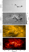 |
Fig. 1. Basic structure of the studied region seen by SDO/HMI and AIA. Top panel: solar surface with HMI continuum observation. Second panel: vertical component of photospheric magnetic field. Bottom two panels: AIA 171 Å and 304 Å images, respectively. The arrows in the panels mark the location of the filament system. The axes are labeled by the heliographic longitude and latitude from the center of solar disk. |
The bottom two panels in Fig. 1 show the AIA observation in two EUV channels, 171 Å and 304 Å, respectively. As can be seen in both channels, a filament system consisting of multiple dark threads (marked by arrows in the figure) nearly runs along the full length of the main PIL, therefore also an inverse-S shape. In the next sections, we show that the filament corresponds to long MFR, lying low above the PIL. The main part of the filament system continuously connects the left δ sunspot to the end of the middle one (as denoted by the right two arrows), while another part is seen in the leftmost of the sunspots (the left arrow). Overlying the filament, there are large-scale closed loops as seen in the 171 Å. The filament system can be clearly seen at as early as 9:00 UT on November 7 and remains stable until the X1.6 flare, even though the AR experiences a few smaller flares over the course of the duration.
3.2. Flare and filament ejection
The X1.6 flare is associated with the eruption of this whole filament system, while the detailed process is complex as shown in Fig. 2 (and its supplementary animation) along with the GOES soft X-ray flux. There are two episodes of dynamic events preceding the major eruption. Firstly, at about 16:00 UT, that is, 1 h before the X1.6 flare onset, along with some degree of expansion and brightening of the overlying loops, the main part of the filament system arched outwards a little bit and became bright, which takes about 15 min (see the top panels of Fig 2, in particular, the filament as pointed out by the arrows). Meanwhile, weak UV ribbons are also seen in the AIA 1600 Å (and 304 Å) images simultaneously at the two δ sunspots, which indicates the occurring of magnetic reconnection there, just below the main filament, possibly in the form of the standard tether-cutting reconnection driven by flux cancellation. The emission of this reconnection is rather weak in the GOES soft X-ray flux, with only a slight bump at 16:10 UT in the light curve (see the supplementary animation of Fig. 2). We note that during this episode, the filament did not erupt but disappeared in the EUV images, possibly due to the heating of the filament materials by the reconnection. This may suggest that the small reconnection activates the filament by enhancing the corresponding MFR, but MFR has not reaches a global instability because the overlying field is strong enough to hold it to a new equilibrium. Another small bump in the light curve of soft X-ray is seen at around 16:40 UT, which indicates the second event of reconnection (see panels in the second row of Fig. 2 and the animation). The corresponding UV ribbons have a round shape located in the south neighboring to the central δ sunspot and is accompanied with a small coronal jet (actually this jet recurred during the evolution of the AR, Zhang et al. 2021). Such a circular ribbon suggests that there should be a null-point like topology (e.g., Masson et al. 2009; Wang & Liu 2012) and indeed the magnetogram shows a parasitic positive polarity enclosed by the main, negative polarity there (see the magnetogram shown in Fig. 1). The second episode of reconnection might be driven by the flux expansion in the first event or due to the internal instability between the parasitic polarity and its surroundings. It seems that again this reconnection did not yet trigger the major eruption of the X1.6 flare, but it may reduce slightly the overlying flux above the main filament. Thus, we conjecture that these two episodes of reconnection did not trigger the global instability of the MFR supporting the filament system, but they may help to build up the MFR to that level of instability. More analyses of this on the basis of the coronal magnetic field is given in Sects. 3.4 and 3.5. We note that the occurrence of small reconnections preceding major flares has also been reported in other papers (e.g., Zhao et al. 2016; Kliem et al. 2021).
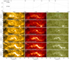 |
Fig. 2. Evolution of the GOES soft X-ray flux during 16:00:00 UT to 18:00:00 UT (top panel) and observation of the X1.6 flare in 171 Å (a1–a6), 304 Å (b1–b6), and 1600 Å (c1–c6) bands. The labels T1 to T6 correspond to the time shown in the following panels. The overlaid contours are shown for Bz = 500 G (colored in cyan) and −500 G (pink) in panels a1, b1 and c1. Arrows in panels a1 and b1 indicate the location of the filament. Arrows in panels a2, b2 and c2 point to the circular ribbon of a C7.0 flare. Arrows in panels a3, b3 and c3 indicate the initiation of the X1.6 flare. Arrows in panel b4 show the rising filament with a helical shape. Arrows in panels a5 and b5 point to the eruption of the filament. An animation of this figure is provided online. |
The major flare appeared 5 min later. The flare brightening, along with a small-scale ejection (likely to be some part of the filament), was initiated on the upper-left δ sunspot at 16:53 UT (see the third row of Fig. 2). However, this small brightening and ejection did not trigger the large-scale eruption immediately, but within a time interval (from 16:53 UT to 17:01 UT) corresponding to a small stepwise rise in the soft X-ray flux before the major rise (see also Yurchyshyn et al. 2015). The major eruption started when the hot loops close to the brightening began to expand at 17:03 UT, as seen in both the AIA 94 Å and 131 Å channels. Meanwhile, the filament rose up quickly, as seen in both 171 Å and 304 Å bands. Within a few minutes around 17:08 UT, it seems to demonstrate a helical shape with at least two places of kink (as denoted by the arrows in the fourth row in Fig. 2 and seen more clearly in the animation), which is likely an evidence of eruption of an MFR and has been invoked to hint that the MFR run into a kink instability (Yurchyshyn et al. 2015). Moreover, in the 131 Å wavelength, a hot channel, although rather diffusive, expanded outwards along with the filament ejection, which is another piece of indirect evidence often invoked to support the eruption of an MFR (Cheng et al. 2017). This filament erupted mainly toward the north-east direction (as denoted by the arrows in the fifth row in Fig. 2) and resulted in a moderate CME with an average speed of 938 km s−1, detected by the SOHO/LASCO C2 coronagraph at 18:08 UT (Yurchyshyn et al. 2015). The resulting effects feature post-flare loops along the main PIL, as well as flare ribbons that are expanded toward both the left and right sides from the initial brightening at the left-top δ sunspot, seen as two long parallel ribbons along the main PIL. We note that at the flare onset, the two ribbons were so close to each other that they almost collided with the main PIL and then they separated quickly thereafter. By the end of the flare, they had swept across the entire polarities of the sunspots, suggesting that a large portion of the magnetic flux was involved in the flare reconnection.
3.3. Evolution of photospheric magnetic field
Before studying the coronal magnetic field, we first looked toward the evolution of the photospheric field for two days between November 6 and 7, shown in Fig. 3 (and its supplementary animation). Although the basic magnetic configuration does not change significantly, the sunspot interactions are dynamic and there are three features in evolution of the magnetograms that are expected to play important roles in building up the MFR of the filament until its eruption. These are, respectively, the rotation of the sunspots, which can be seen most clearly in the upper-left δ sunspots, the shearing movement between the opposite polarities, which is most clearly seen in the central elongated δ sunspots, and the cancellation of the magnetic flux around the main PIL. Using the DAVE4VM code (Schuck 2008), we computed the velocity of the photospheric flows from the time sequence of vector magnetograms and the typical flow pattern are shown in Fig. 3 panels d and e. Panel d corresponds to the upper-left δ sunspot region as boxed by the green rectangle A in panel a, and this is the site of the X1.6 flare initiation. The sunspot with negative polarity shows clockwise rotation, forming a vortex centered at the sunspot center. The positive spot also shows a rotation in the same direction but not that evident as the negative one. This rotation persisted for hours before the eruption, which is likely the result of a new flux emergence that was studied in detail by Yurchyshyn et al. (2015). We note that the X1.6 flare is triggered at exactly the PIL of this rotating sunspot, suggesting that a current sheet is formed there as driven by the magnetic shear at the PIL owing to the sunspot rotation. Panel e is the close view of the central δ sunspot, namely, the red boxed region B in panel a, and we can see there is obvious shearing motion between the positive polarity (going left) and negative polarity (going right). Furthermore, in Fig. 3f, we show the evolution of magnetic flux of the positive polarity in this region, since this polarity is well isolated with others and we can see a systematic decrease of the flux, which indicates a continuous flux cancellation along the main PIL. About 40% of the flux is cancelled until the onset of the eruption, which is similar to the value reported by Green et al. (2011) for AR 10977. It is well known that all these motions and flux cancellation can build up non-potentiality and, in particular, MFR in the corona (Green et al. 2011; Yardley et al. 2018). Consequently, the horizontal field near the PIL is mostly aligned with the PIL (see the supplementary animation of Fig. 3), thus, there is a strong sheared magnetic configuration.
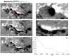 |
Fig. 3. Evolution of the photospheric magnetic field. The boxed regions labeled with A and B in panel a correspond to the fields of view in panel d and panel e, respectively. Panel f: evolution of the positive magnetic flux in the red box in panel a. An animation of this figure is provided online. |
3.4. Structure and evolution of the 3D coronal magnetic field
To study the coronal magnetic field and its evolution, we reconstruct the coronal magnetic fields from the HMI vector magnetograms using the CESE–MHD–NLFFF code. In particular, a time sequence of the coronal fields is reconstructed from 00:00 UT to 20:00 UT with time cadence of 1 h, and within the 2 h around the flare onset, the cadence is reduced to 12 min for a more detailed evolution that might be associated with the localized reconnection events before the main eruption. We note that for a coronal field reconstruction of good quality, the vector magnetogram should be observed close to the solar disk center, for example, within ±45° from the central meridian, so the measurement errors of the photospheric vector field may be small. However, the studied AR only rotated into −45° around the time of the X1.6 flare and thus it is a challenge to reconstruct the long time pre-flare evolution of the coronal field. Nevertheless, from the reconstructed field, a large-scale long-existing MFR along the PIL is found to be associated with the aforementioned filament.
To illustrate the 3D structure of the MFR, we display the sampled magnetic field lines and the 3D distribution of magnetic twist number in the volume, as well as the current density distribution in Fig. 4 for three representative times before the eruption and one after. The panels in the left column show the magnetic field lines with different colors, and as we can see, the magnetic field lines wind around each other, forming a highly twisted MFR. The MFR has a positive helicity with right-handed twist, which is against the hemisphere handedness rule for an AR in the northern hemisphere. The two middle columns show 3D iso-surface with magnetic twist number Tw = 1 in two different view angles, respectively. The iso-surface of Tw = 1 is a surface of a volume in which the magnetic twist numbers of all the field lines exceed 1, a threshold used to define the existence of MFR in our previous work (Duan et al. 2019, 2021a). Moreover, the iso-surface is pseudo-colored by the value of height. By comparing the structures at different times, we can see that prior to the X1.6 flare, the MFR grows thicker and thicker, with a rise in the twist degree and height. While after the flare (see panels at 18:00 UT), the field reconfigures substantially to a much thinner MFR if compared with the pre-flare one, suggesting that the pre-flare thick MFR had indeed erupted during the flare. As the MFR is a manifestation of the electric currents in the corona, we also plot the vertical integral of the current density along the height in the right column in Fig. 4. It also shows a similar structure and evolution as that of the volume of the MFR; the current concentrates around the PIL, which is the region where the MFR resides, expands before the flare and has an obvious shrinkage after the flare.
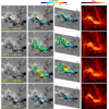 |
Fig. 4. Structure and evolution of the MFR and the current density before to after the X1.6 flare. Left column: sampled magnetic field lines shown with different colors for a better view of each field line. Two middle columns: Iso-surface of magnetic twist number Tw = 1 in the x − y plane and in 3D, the structure is false-colored by the value of height z in units of arcsecond (or 720 km). Right column: evolution of the current distribution which is calculated by integration of the current density along the z direction. |
In Fig. 5, we give a more detailed structure and evolution of the MFR by showing the distribution of twist number at a vertical cross section of the MFR. This cross-section cuts through the MFR at its middle part of the main PIL (i.e., the part in the central δ sunspot), which is denoted by the red line on the top panel in Fig. 4. As can be seen, the twist distribution in the MFR is rather non-uniform and asymmetric but overall it forms a coherent structure within Tw > 1, which grows in size before the flare and shrinks quickly across the flare. In Appendix B, we show more details of the field lines and the field vectors at the cross-section, which demonstrate that the field line with the largest Tw is a good proxy of the axis of the MFR; also Tw approximates the winding number of the field line near the axis reasonably well. To give a quantitative variation of the MFR, we calculated the total toroidal (or axial) flux of the MFR by summing up all the flux through the cross-section with twist number Tw > 1, which is shown in the bottom panel of Fig. 5. We note that here the toroidal flux does not contain those outside the MFR, although the outside flux is sheared and thus has toroidal component. We can see that the MFR’s toroidal flux increases overall, from initially about 1020 Mx to 2.5 × 10²⁰ Mx just before the flare, although the increasing trend is interrupted several times, possibly owing to the other smaller flares preceding the X1.6 one and also due to uncertainties in the NLFFF extrapolation that are introduced by the measurement errors of vector magntograms, the preprocessing, and the NLFFF code itself. We note that the toroidal flux increases most prominently in a few hours immediately before the major flare. Then it drops quickly after the flare (marked by the grey box on the figure) to a value of ∼0.5 × 10²⁰ Mx, confirming again that the MFR erupted during the flare.
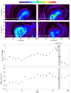 |
Fig. 5. Evolution of twisted flux of the MFR. Top and middle: evolution of the twist number of the MFR on the cross section whose location is denoted by the red line on the top-middle panel in Fig. 4. Bottom: toroidal magnetic fluxes of the MFR computed on the same cross section, and the fluxes are integrated with only those having Tw ≥ 1. |
The correlation of the MFR with the flare eruption is further supported thanks to a study of the magnetic topology of the MFR. Theoretical analyses of coronal MFR show that the MFR is wrapped by a magnetic quasi-separatrix layer (QSL) separating the MFR from its ambient field (Titov et al. 2002). In addition, flare reconnection occurs essentially within this QSL during eruption of the MFR (Aulanier et al. 2010; Jiang et al. 2018). As a result, the flare ribbons map the footprints of the QSL at the photosphere. If the MFR is initially low-lying and touches the solar surface, the QSL is actually a bald batch separatrix surface and the footprints of the QSL coincide with the PIL. With the fast rising of the MFR, the bald batch separatrix surface quickly evolves into a hyperbolic flux tube, and the QSL footprints bifurcate into two parallel ribbons that depart away from each other with respect to the PIL. In Fig. 6, we compare the flare ribbons in 1600 Å and the distribution of the magnetic squashing degree (or Q factor) and the twist number at the photosphere for the reconstructed field at time of 17:00 UT, a few minutes before the X1.6 flare. The Q factor is defined as a quantity to measure the shape distortions of the elemental flux tubes based on the field-line mapping (Demoulin et al. 1996; Titov et al. 2002) and a high value of Q (e.g., ∼105) indicates a steep gradient of the field-line mapping, which always occurs in QSLs. As can be seen, the twisted flux is most enhanced along the main PIL and the QSL footprints of the pre-flare MFR, which is indicated by extremely narrow areas with high Q of around 105 – almost forming a thin line coinciding with the main PIL. This suggests that the body of the MFR is nearly attached to the photosphere. If the MFR erupts, the QSL footprints naturally bifurcate into two ribbons. This is highly consistent with the structure and evolution of the flare ribbons, of which two ribbons are initially so close to each other that they almost coincide with the main PIL just before separating.
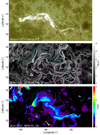 |
Fig. 6. Flare ribbons in 1600 Å (top panel), the squashing degree (Q factor, middle panel), and the twist number distribution (bottom panel) around the PIL before the X1.6 flare peak. |
3.5. Instability of the MFR
It has been suggested that the MFR becomes unstable and erupts, as manifested by the filament eruption. Thus, we further analyze why the MFR became unstable. To this end, we resorted to the two kinds of classical instability: the kink instability and the torus instability. We measured the twist degree (in both Tw and 𝒯) in the MFR as well as the decay index of the strapping field at the field line with the largest twist number, which is assumed to be the axis of the MFR.
Figure 7a shows the evolution from 00:00 UT to 20:00 UT of four parameters: the largest twist number (Tw)max, the average twist number (Tw)mean, the largest winding number 𝒯max, and the average winding number 𝒯mean of the MFR. We note that there are systematic differences between Tw and 𝒯, with the latter lower than the former by around 0.4 turns. Figure 7 panels b and c show that of the decay index and height of the MFR axis for two locations: we calculated the decay index at two locations because the MFR axis is rather long and serpentine; we found there are two apex points, one above the upper-left δ sunspot and the other above the central δ sunspot, respectively. Furthermore, the overlying fields at these two locations are stronger than elsewhere along the path of the MFR and should play the major role in the confinement of the MFR. Therefore, the decay index as well as the height are computed for these two places. The question of whether the MFR is torus unstable can be explored more thoroughly. Specifically, the parameters displayed in Fig. 7b are calculated in region A in Fig. 3a as well as the intersection point of the magenta line and the MFR shown in the top panel of Fig. 4. The parameters shown in Fig. 7c are for region B in Fig. 3a, and the point which the red line intersects with the MFR shown in the top panel of Fig 4. All the parameters are calculated with a cadence of 12 min around the flare (from 16:00 UT to 18:00 UT) and 1 h otherwise.
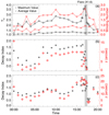 |
Fig. 7. Evolution of the twist number Tw, the winding number 𝒯 (including both their largest value and mean value), the decay index, and height of the MFR axis. Parameters in panels b and c are calculated from different positions of the MFR, where panel b corresponds to region A in Fig. 3a (also to the point of intersection between the magenta line and the MFR on the middle-top panel in Fig. 4), panel c corresponds to region B in Fig. 3a (and the point where the red line intersects with the MFR on the middle-top panel in Fig. 4). The height z is in unit of arcsecond (or 720 km). |
From the largest twist number and winding number, we can see that an MFR exists nearly the entire time since these two parameters are almost always above 1. Overall, the largest twist number and winding number are maintained at the level of around 2.5 and 2, respectively, before the X1.6 flare, although there are several fluctuations, for example, in the initial few hours, and also around 10:00 UT. These fluctuations, similar to those shown in the evolution of the toroidal flux (bottom panel of Fig. 5), might be partially caused by uncertainties in the NLFFF extrapolations; for example, the measurement errors of vector magntograms are large since the AR is far away from the central meridian in the initial hours (it only rotates to −45° around the time of the X1.6 flare). The smaller flares preceding the X1.6 flare may also have induced variations to the MFR and resulted in fluctuations of (Tw)max. For example, the one around 10:00 UT is likely due to the M1.0 flare at that time. Noticeably, within about 1 h before the flare, the largest twist number and winding number increase rather fast and reach close to 3.8 and 2.6 just before the X1.6 flare, and then drop quickly across the flare to a value fairly below 2. We conjecture that the fast increase of the twist number might be due to the first small reconnection event in 1 hour prior to the major eruption, which enhances the twist degree of the MFR, through a tether-cutting process. This is consistent with the finding of Liu et al. (2016) and Duan et al. (2021a) that states that the MFR’s maximum twist number is sensitive to variations in the MFR through eruptions. Although both the largest value of twist and winding numbers suggest a possible kink instability, their averaged values that quantify the large-scale twist of the MFR are smaller (with pre-flare values of (Tw)mean = 1.2 and 𝒯mean = 0.9) and below the smallest threshold for kink instability, namely 1.25 (Hood & Priest 1981), which seems to against the onset of kink instability during the eruption.
The decay index provides valuable information, as shown in the last two panels of Fig. 7, indicating that the constraining field of the MFR decreases with height fast enough to trigger the torus instability. Clearly there is an overall ascension of the MFR axis and, thus, an increase in the decay index, in both two locations above the two δ sunspots, prior to the X1.6 flare. In particular, above the central part of the main PIL (i.e., the central δ sunspot), the MFR axis reaches a height of 22 arcsec (or 16 Mm), which even exceeds the extension of the main polarities across the main PIL. This naturally indicates a large decay index of the strapping field as approximated by the corresponding potential field. Thus, the decay index closely before the flare is well above the canonical threshold (i.e., 1.5) of torus instability (Kliem & Török 2006). Also, in the left part of the MFR, the decay index reaches above 1.5. Therefore, we suggest that the MFR could be subject to the torus instability in the eruption. Both the decay index and the height decrease rapidly after the flare since the field is reconfigured substantially with the eruption of the pre-flare MFR. We note that there is no data after 18:00 UT in Fig. 7b because the left part of the MFR simply disappeared after 18:00 UT.
3.6. Evolution of magnetic energy and helicity
Finally, we studied the evolution of magnetic energies and relative helicity, calculated for the whole AR since the flare resulted in a global disruption of the region. The results are shown in Fig. 8, including the evolution of the total unsigned flux of the whole region. Both the total magnetic energy EN and the potential magnetic energy EP show a slow decrease before the X1.6 flare. This is consistent with the gradual decline of the total magnetic flux. The total energy before the flare is about double of the potential field energy, which indicates that the AR is strongly non-potential in character. This is also shown by the non-potentiality parameter EF/EP, which increases mildly in a few hours before the flare and reaches around 1.3. We note that the ratio EF/EP of ∼1.3 is much larger than those reported in some previous works based on other NLFFF codes for different ARs. For example, Schrijver et al. (2008) calculated the magnetic energies for AR 10930 using different NLFFF codes and found that the largest one obtained from all their different NLFFF models is ∼0.5. Sun et al. (2015) used Wiegelmann’s code for three different ARs to show that the ratio is ∼0.3 for AR 11158, ∼0.5 for AR 11429, and ∼0.03 for AR 12192, respectively. However, MHD models of eruptions that use a self-consistent way to inject free energy via surface driving to eventually initiate an eruption show that the ratio often needs to reach a value around 1.0 ∼ 1.5 to initiate an eruption (Amari et al. 2003, 2010, 2011; Jiang et al. 2021; Zuccarello et al. 2015). Our result is consistent with these simulations. Across the flare, the total magnetic energy drops quickly from 1.2 × 1033 erg to approximately 1033 erg, while the potential field energy varies only slightly. Consequently, the free magnetic energy across the flare drops from 0.7 × 1033 erg to 0.45 × 1033 erg, which means that magnetic energy of 3.5 × 1032 erg is released by the flare eruption. Such an amount of magnetic energy is sufficient to power a typical X-class flare according to previous estimations of flare energy budget (Emslie et al. 2012). The non-potentiality indicator EF/EP decreases significantly from above 1.3 to below 0.9. Nevertheless, it also suggests that the post-flare field is still rather non-potential, which is consistent with the facts that the horizontal field along the main PIL is still strongly sheared and that an MFR exists after the flare. The relative magnetic helicity exhibits an evolution trend, namely, an overall increase before the flare and a sharp decrease after the flare. This trend is rather similar to that of the total toroidal flux of the MFR (Fig. 5) and its largest twist number (Fig. 7), suggesting that the helicity is closely related to the twisted flux of the MFR. We note that the helicity well after the flare is actually negative, thus suggesting that the full region before the flare contains both signs of helicity and the MFR stores the major positive one. The helicity normalized by the square of the unsigned magnetic flux evolves also in the same way, with a highest value of about 0.025 immediately before the flare and dropping to 0.005 after the flare. All these evolutions of non-potentiality and helicity are in accordance with the eruption of an MFR during the flare. Finally, we ought to highlight, again, that all these numbers of magnetic energies and helicity contain uncertainties that are introduced by the measurement errors of vector magntograms, the preprocessing, and the NLFFF code itself. For example, there is a relative error of about 5% as introduced by the numerical magnetic divergence to the free energy (see Appendix A).
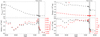 |
Fig. 8. Evolution of the unsigned magnetic flux, the relative helicity, and the energy computed on the AR 12205 region from 00:00 UT to 20:00 UT on 2014 November 7. |
4. Conclusions and discussion
In this paper, we comprehensively study the magnetic field and evolution associated with a major flare eruption in solar AR 12205, based mainly on the observations from the SDO and coronal magnetic field extrapolations. The AR is characterized by a long sequence of sunspots aligned in the longitudinal direction on the Sun, harboring two groups of δ sunspots that evolved dynamically by continual rotation (associated with flux emergence), shearing, colliding, and flux cancellation. As a result, a strong sheared and high-gradient PIL was formed between opposite polarities of the sunspots. Thanks to the joint effect of the sunspot motions, a large-scale MFR with length of about 200 Mm was gradually built up along the main PIL, which is evidenced by the corresponding long filament and the coronal field reconstruction. Our detailed analysis of the coronal magnetic evolution indicates that the torus instability of the MFR is the most likely mechanism that finally led to the major eruption of the X1.6 flare, although it was preceded by episodes of localized reconnections. We suggest that these localized reconnections should play an important role in enhancing the pre-flare MFR by, for example, tether-cutting reconnection low near the photosphere as driven by the shearing and flux cancellation. Thus, the study of this event supports many earlier flux-emergence and flux cancellation MHD simulations in which pre-eruptive tether-cutting reconnection forms a flux rope and drives it upward up to an instability (e.g., Manchester et al. 2004; Aulanier et al. 2010; Amari et al. 2010; Zuccarello et al. 2015; Syntelis et al. 2017). The analysis of the evolution of the magnetic twist of the MFR suggests that the pre-eruptive MFR has its largest twist of approximately three turns but a moderate twist degree of about one turn (around its axis), on average, which does not support the kink instability. This emphasizes the importance of calculating the large-scale twist rather than only a local twist on the axis for a more comprehensive judgement of kink instability. On the other hand, the decay index of its strapping field suggests that the MFR was lifted up to a height close to torus unstable, at which the background restraining force is weak enough. Then it erupted unavoidably and escaped into the space as a CME, leaving two long flare ribbons that were initially consistent in shape with the footprints of the QSL wrapping the pre-flare MFR and then quickly separated from each other with the fast rising of the MFR. Further calculations suggest that an amount of about 2 × 1032 erg of the magnetic energy and about 1 × 1043 Mx2 of magnetic helicity was released by the flare.
A previous study of the same event by Yurchyshyn et al. (2015) was based on multi-wavelength analysis but without an analysis of the coronal magnetic field, and led those authors to a similar conclusion: a series of pre-flare reconnections involving different magnetic flux systems leads to the formation of an unstable flux rope, which then erupts by the torus instability, possibly (and also the kink instability). Our study supports this finding (except the kink instability) based on a detailed analysis of the coronal magnetic field structure and evolution. Our study further shows that the MFR actually exists (by at least 10 h) well before the eruption – rather than immediately formed before its eruption as conjectured by Yurchyshyn et al. (2015) and it experienced a few smaller flares and thus reconnections, confirming that the key initiation mechanism of its eruption is not reconnection. This is consistent with the study of two flares in another active region, namely AR 12673 (Zou et al. 2019, 2020). On September 6, 2017, that AR produced an X2.2 confined flare and an X9.3 eruptive flare from the same PIL within a short time interval of only about 2 hours. Both flares are found to be associated with the same pre-existing MFR, while the key difference between them is that for the confined flare, the MFR is far below the threshold of torus instability, whereas for the eruptive one, the MFR reaches entirely above the threshold, which provides a strong indication that it is the ideal instability, rather than the reconnection, that plays a decisive role in initiating the eruption. A rather interesting characteristic of evolution is that the MFR is built up quite rapidly to torus instability with its height lifted up substantially within only about 1 hour preceding the X9.3 flare, presumably through a recurring null-point reconnection neighboring to the MFR (Zou et al. 2020). This is very similar to the studied event here, as the height of the MFR in its central part increased substantially within a short time immediately before its eruption, which is also likely via localized reconnections in the corona. This indicates that such localized reconnections could very efficiently build up an unstable MFR shortly before its eruption. Our findings are also consistent with a recent study by Kliem et al. (2021) of a compound eruptive event in AR 12371, in which a series of preceding confined flares across a short time interval (of less than 1 hour) before an eruptive flare play a key role in building up an unstable MFR that initiated the final eruption. These authors suggested that the enhancement of MFR by the preceding confined flares might be a generic process occurring prior to many CMEs, which is a finding that is supported by the present study. The question of whether such pattern of MFR evolution prior to eruption is common in other ARs and events will be left to future investigations.
Movies
Movie 1 associated with Fig. 2 (fig2_animation) Access Supplementary Material
Movie 2 associated with Fig. 3 (fig3_animation) Access Supplementary Material
It should be noted that there are cases in which the MFR axis is located at a local minimum of |Tw|; for example, consider a so-called hollow-core rope, in which the current density is enhanced mostly near the outer layer. Such cases often occur in decayed ARs and the quiet Sun (e.g., Su et al. 2011).
Acknowledgments
This work is supported by National Natural Science Foundation of China (NSFC) U2031108 and Guangdong Basic and Applied Basic Research Foundation (2021A1515011430). C.J. acknowledges support by NSFC 4217040250, 41822404, 41731067. The computational work of the NLFFF extrapolations was carried out on TianHe-1(A), National Supercomputer Center in Tianjin, China. Data from observations are courtesy of NASA/SDO. Special thanks to our anonymous reviewer for valuable suggestions that helped improve the paper.
References
- Alt, A., Myers, C. E., & Ji, H. 2021, ApJ, 908, 41 [NASA ADS] [CrossRef] [Google Scholar]
- Amari, T., Canou, A., & Aly, J. J. 2014, Nature, 514, 465 [NASA ADS] [CrossRef] [Google Scholar]
- Amari, T., Luciani, J. F., Aly, J. J., Mikic, Z., & Linker, J. 2003, ApJ, 585, 1073 [NASA ADS] [CrossRef] [Google Scholar]
- Amari, T., Aly, J.-J., Mikic, Z., & Linker, J. 2010, ApJ, 717, L26 [NASA ADS] [CrossRef] [Google Scholar]
- Amari, T., Aly, J.-J., Luciani, J.-F., Mikic, Z., & Linker, J. 2011, ApJ, 742, L27 [NASA ADS] [CrossRef] [Google Scholar]
- Antiochos, S. K., DeVore, C. R., & Klimchuk, J. A. 1999, ApJ, 510, 485 [Google Scholar]
- Archontis, V., & Hood, A. W. 2010, A&A, 514, A56 [NASA ADS] [CrossRef] [EDP Sciences] [Google Scholar]
- Aschwanden, M. J., Xu, Y., & Jing, J. 2014, ApJ, 797, 50 [Google Scholar]
- Aulanier, G., Török, T., Démoulin, P., & DeLuca, E. E. 2010, ApJ, 708, 314 [Google Scholar]
- Baty, H. 2001, A&A, 367, 321 [NASA ADS] [CrossRef] [EDP Sciences] [Google Scholar]
- Berger, M. A., & Field, G. B. 1984, J. Fluid Mech., 147, 133 [NASA ADS] [CrossRef] [Google Scholar]
- Berger, M. A., & Prior, C. 2006, J. Phys. A Math. Gen., 39, 8321 [Google Scholar]
- Bleybel, A., Amari, T., van Driel-Gesztelyi, L., & Leka, K. D. 2002, A&A, 395, 685 [NASA ADS] [CrossRef] [EDP Sciences] [Google Scholar]
- Bobra, M. G., Sun, X., Hoeksema, J. T., et al. 2014, Sol. Phys., 289, 3549 [Google Scholar]
- Chen, J. 1989, ApJ, 338, 453 [NASA ADS] [CrossRef] [Google Scholar]
- Chen, P. F. 2011, Liv. Rev. Sol. Phys., 8, 1 [Google Scholar]
- Cheng, X., Guo, Y., & Ding, M. 2017, Sci. Chin. Earth Sci., 60, 1383 [NASA ADS] [CrossRef] [Google Scholar]
- Dellar, P. J. 2001, J. Comput. Phys., 172, 392 [NASA ADS] [CrossRef] [Google Scholar]
- Démoulin, P., & Aulanier, G. 2010, ApJ, 718, 1388 [Google Scholar]
- Demoulin, P., Henoux, J. C., Priest, E. R., & Mandrini, C. H. 1996, A&A, 308, 643 [NASA ADS] [Google Scholar]
- DeRosa, M. L., Schrijver, C. J., Barnes, G., et al. 2009, ApJ, 696, 1780 [NASA ADS] [CrossRef] [Google Scholar]
- Duan, A., Jiang, C., Hu, Q., et al. 2017, ApJ, 842, 119 [NASA ADS] [CrossRef] [Google Scholar]
- Duan, A., Jiang, C., He, W., et al. 2019, ApJ, 884, 73 [NASA ADS] [CrossRef] [Google Scholar]
- Duan, A., Jiang, C., Toriumi, S., & Syntelis, P. 2020, ApJ, 896, L9 [NASA ADS] [CrossRef] [Google Scholar]
- Duan, A., Jiang, C., Zhou, Z., Feng, X., & Cui, J. 2021a, ApJ, 907, L23 [NASA ADS] [CrossRef] [Google Scholar]
- Duan, A., Jiang, C., Zou, P., Feng, X., & Cui, J. 2021b, ApJ, 906, 45 [NASA ADS] [CrossRef] [Google Scholar]
- Emslie, A. G., Dennis, B. R., Shih, A. Y., et al. 2012, ApJ, 759, 71 [Google Scholar]
- Fan, Y. 2010, ApJ, 719, 728 [NASA ADS] [CrossRef] [Google Scholar]
- Fan, Y., & Gibson, S. E. 2003, ApJ, 589, L105 [NASA ADS] [CrossRef] [Google Scholar]
- Fan, Y., & Gibson, S. E. 2007, ApJ, 668, 1232 [Google Scholar]
- Finn, J. M. 1984, Comments. Plasma Phys. Controlled Fusion, 9, 111 [NASA ADS] [Google Scholar]
- Forbes, T. G., Linker, J. A., Chen, J., et al. 2006, Space Sci. Rev., 123, 251 [Google Scholar]
- Fuhrmann, M., Seehafer, N., & Valori, G. 2007, A&A, 476, 349 [NASA ADS] [CrossRef] [EDP Sciences] [Google Scholar]
- Green, L. M., Kliem, B., & Wallace, A. J. 2011, A&A, 526, A2 [NASA ADS] [CrossRef] [EDP Sciences] [Google Scholar]
- Guo, Y., Zhong, Z., Ding, M. D., et al. 2021, ApJ, 919, 39 [NASA ADS] [CrossRef] [Google Scholar]
- Hood, A. W., & Priest, E. R. 1981, Geophys. Astrophys. Fluid Dyn., 17, 297 [NASA ADS] [CrossRef] [Google Scholar]
- Inoue, S. 2016, Prog. Earth Planet. Sci., 3, 19 [CrossRef] [Google Scholar]
- Inoue, S., Hayashi, K., Magara, T., Choe, G. S., & Park, Y. D. 2014, ApJ, 788, 182 [NASA ADS] [CrossRef] [Google Scholar]
- Inoue, S., Kusano, K., Büchner, J., & Skála, J. 2018, Nat. commun., 9, 174 [CrossRef] [Google Scholar]
- Jiang, C., Duan, A., Feng, X., et al. 2019, Front. Astron. Space Sci., 6, 63 [NASA ADS] [CrossRef] [Google Scholar]
- Jiang, C. W., & Feng, X. S. 2012, ApJ, 749, 135 [NASA ADS] [CrossRef] [Google Scholar]
- Jiang, C., & Feng, X. 2013, ApJ, 769, 144 [NASA ADS] [CrossRef] [Google Scholar]
- Jiang, C., & Feng, X. 2014, Sol. Phys., 289, 63 [NASA ADS] [CrossRef] [Google Scholar]
- Jiang, C.-W., & Feng, X.-S. 2016, Res. Astron. Astrophys., 16, 015 [CrossRef] [Google Scholar]
- Jiang, C. W., Feng, X. S., Zhang, J., & Zhong, D. K. 2010, Sol. Phys., 267, 463 [NASA ADS] [CrossRef] [Google Scholar]
- Jiang, C., Wu, S. T., Feng, X., & Hu, Q. 2014, ApJ, 786, L16 [NASA ADS] [CrossRef] [Google Scholar]
- Jiang, C., Zou, P., Feng, X., et al. 2018, ApJ, 869, 13 [NASA ADS] [CrossRef] [Google Scholar]
- Jiang, C., Feng, X., Liu, R., et al. 2021, Nat. Astron., 5, 1126 [NASA ADS] [CrossRef] [Google Scholar]
- Jing, J., Chen, P. F., Wiegelmann, T., et al. 2009, ApJ, 696, 84 [Google Scholar]
- Jing, J., Tan, C., Yuan, Y., et al. 2010, ApJ, 713, 440 [NASA ADS] [CrossRef] [Google Scholar]
- Jing, J., Liu, C., Lee, J., et al. 2018, ApJ, 864, 138 [NASA ADS] [CrossRef] [Google Scholar]
- Kliem, B., & Török, T. 2006, Phys. Rev. Lett., 96 [Google Scholar]
- Kliem, B., Lee, J., Liu, R., et al. 2021, ApJ, 909, 91 [NASA ADS] [CrossRef] [Google Scholar]
- Kuperus, M., & Raadu, M. A. 1974, A&A, 31, 189 [NASA ADS] [Google Scholar]
- Lemen, J. R., Title, A. M., Akin, D. J., et al. 2012, Sol. Phys., 275, 17 [Google Scholar]
- Liu, R., Kliem, B., Titov, V. S., et al. 2016, ApJ, 818, 148 [Google Scholar]
- Low, B. C., & Lou, Y. Q. 1990, ApJ, 352, 343 [NASA ADS] [CrossRef] [Google Scholar]
- Luoni, M. L., Démoulin, P., Mandrini, C. H., & Driel-Gesztelyi, L. V. 2011, Sol. Phys., 270, 45 [NASA ADS] [CrossRef] [Google Scholar]
- Malanushenko, A., Schrijver, C. J., DeRosa, M. L., & Wheatland, M. S. 2014, ApJ, 783, 102 [Google Scholar]
- Manchester, W. B., Gombosi, T. I., Roussev, I., et al. 2004, J. Geophys. Res., 109, 2107 [Google Scholar]
- Masson, S., Pariat, E., Aulanier, G., & Schrijver, C. J. 2009, ApJ, 700, 559 [Google Scholar]
- McCauley, P. I., Su, Y. N., Schanche, N., et al. 2015, Sol. Phys., 290, 1703 [NASA ADS] [CrossRef] [Google Scholar]
- Moore, R. L., Sterling, A. C., Hudson, H. S., & Lemen, J. R. 2001, ApJ, 552, 833 [Google Scholar]
- Myers, C. E., Yamada, M., Ji, H., et al. 2015, Nature, 528, 526 [Google Scholar]
- Pariat, E., Leake, J. E., Valori, G., et al. 2017, A&A, 601, A125 [CrossRef] [EDP Sciences] [Google Scholar]
- Pesnell, W. D., Thompson, B. J., & Chamberlin, P. C. 2012, Sol. Phys., 275, 3 [Google Scholar]
- Régnier, S. 2013, Sol. Phys., 288, 481 [CrossRef] [Google Scholar]
- Schou, J., Scherrer, P. H., Bush, R. I., et al. 2012, Sol. Phys., 275, 229 [Google Scholar]
- Schrijver, C. J. 2007, ApJ, 655, L117 [Google Scholar]
- Schrijver, C. J., De Rosa, M. L., Metcalf, T. R., et al. 2006, Sol. Phys., 235, 161 [NASA ADS] [CrossRef] [Google Scholar]
- Schrijver, C. J., DeRosa, M. L., Metcalf, T., et al. 2008, ApJ, 675, 1637 [Google Scholar]
- Schuck, P. W. 2008, ApJ, 683, 1134 [NASA ADS] [CrossRef] [Google Scholar]
- Shibata, K., & Magara, T. 2011, Liv. Rev. Sol. Phys., 8, 6 [Google Scholar]
- Su, Y., Surges, V., van Ballegooijen, A., DeLuca, E., & Golub, L. 2011, ApJ, 734, 53 [Google Scholar]
- Sun, X., Bobra, M. G., Hoeksema, J. T., et al. 2015, ApJ, 804, L28 [Google Scholar]
- Syntelis, P., Archontis, V., & Tsinganos, K. 2017, ApJ, 850, 95 [NASA ADS] [CrossRef] [Google Scholar]
- Thalmann, J. K., Moraitis, K., Linan, L., et al. 2019, ApJ, 887, 64 [Google Scholar]
- Titov, V. S., & Démoulin, P. 1999, A&A, 351, 707 [NASA ADS] [Google Scholar]
- Titov, V. S., Hornig, G., & Démoulin, P. 2002, J. Geophys. Res., 107, 1164 [Google Scholar]
- Török, T., & Kliem, B. 2003, A&A, 406, 1043 [NASA ADS] [CrossRef] [EDP Sciences] [Google Scholar]
- Török, T., & Kliem, B. 2005, ApJ, 630, L97 [Google Scholar]
- Török, T., & Kliem, B. 2007, Astron. Nachr., 328, 743 [CrossRef] [Google Scholar]
- Török, T., Kliem, B., & Titov, V. S. 2004, A&A, 413, L27 [NASA ADS] [CrossRef] [EDP Sciences] [Google Scholar]
- Török, T., Berger, M. A., & Kliem, B. 2010, A&A, 516, A49 [NASA ADS] [CrossRef] [EDP Sciences] [Google Scholar]
- Valori, G., Démoulin, P., Pariat, E., & Masson, S. 2013, A&A, 553, A38 [NASA ADS] [CrossRef] [EDP Sciences] [Google Scholar]
- van Ballegooijen, A. A. 2004, ApJ, 612, 519 [NASA ADS] [CrossRef] [Google Scholar]
- Vasantharaju, N., Vemareddy, P., Ravindra, B., & Doddamani, V. H. 2018, ApJ, 860, 58 [NASA ADS] [CrossRef] [Google Scholar]
- Wang, H., & Liu, C. 2012, ApJ, 760, 101 [Google Scholar]
- Wiegelmann, T. 2004, Sol. Phys., 219, 87 [NASA ADS] [CrossRef] [Google Scholar]
- Wiegelmann, T., Inhester, B., & Sakurai, T. 2006, Sol. Phys., 233, 215 [Google Scholar]
- Wiegelmann, T., Thalmann, J. K., Inhester, B., et al. 2012, Sol. Phys., 67 [Google Scholar]
- Yardley, S. L., Green, L. M., Driel-Gesztelyi, L. V., Williams, D. R., & Mackay, D. H. 2018, ApJ, 866, 8 [NASA ADS] [CrossRef] [Google Scholar]
- Yurchyshyn, V., Kumar, P., Cho, K. S., Lim, E. K., & Abramenko, V. I. 2015, ApJ, 812, 172 [NASA ADS] [CrossRef] [Google Scholar]
- Zhang, Y.-J., Zhang, Q.-M., Dai, J., Xu, Z., & Ji, H.-S. 2021, Res. Astron. Astrophys., 21, 262 [Google Scholar]
- Zhao, J., Gilchrist, S. A., Aulanier, G., et al. 2016, ApJ, 823, 62 [Google Scholar]
- Zhong, Z., Guo, Y., & Ding, M. D. 2021, Nat. Commun., 12, 2734 [NASA ADS] [CrossRef] [Google Scholar]
- Zou, P., Jiang, C., Feng, X., et al. 2019, ApJ, 870, 97 [NASA ADS] [CrossRef] [Google Scholar]
- Zou, P., Jiang, C., Wei, F., et al. 2020, ApJ, 890, 10 [Google Scholar]
- Zuccarello, F. P., Aulanier, G., & Gilchrist, S. A. 2015, ApJ, 814, 126 [Google Scholar]
- Zuccarello, F., Guglielmino, S. L., Capparelli, V., et al. 2020, ApJ, 889, 65 [NASA ADS] [CrossRef] [Google Scholar]
Appendix A: Quality of the NLFFF extrapolation
Ideally, an NLFFF extrapolation should be perfectly force-free and divergence-free, but in actual implementation with realistic magnetograms, it is subject to numerical errors that are often not negligible. We checked the quality of force-freeness and divergence-freeness of the extrapolated field with two routinely used metrics (e.g., Schrijver et al. 2006; DeRosa et al. 2009; Jiang & Feng 2013). The first is the mean sine of the angle between current J and magnetic field B weighted by J, which is called CWsin and defined as
 (A.1)
(A.1)
where B = |B|, J = |J| and V is the computational volume. The other is the normalized divergence error ⟨|fi|⟩:
 (A.2)
(A.2)
Theoretically, these two metrics vanish in an exact or a perfect force-free field; thus, the smaller the metrics, the better the quality of a field extrapolated from a NLFFF model.
The top panel of Figure A.1 shows the evolution of the CWsin and ⟨|fi|⟩ during 00:00 UT to 20:00 UT on 2014 November 7. Here the black and red dashed lines are average values of CWsin and ⟨|fi|⟩, respectively. We can see that the force-freeness metric CWsin varies from 0.239 to 0.282, and has an average value of 0.253. Meanwhile, the divergence-freeness ⟨|fi|⟩ has values between 3.95 × 10⁻⁴ to 4.65 × 10⁻⁴, and averaged at 4.35 × 10⁻⁴. Both metrics are reasonably small, and consistent with our previous works (Jiang & Feng 2013; Duan et al. 2017, 2021b), indicating a good quality of our extrapolation result.
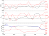 |
Fig. A.1. Evolution of the CWsin and ⟨|fi|⟩ during 00:00 UT to 20:00 UT on 2014 November 7, shown in the top panel. CWsin and ⟨|fi|⟩ are metrics to measure the quality of force-freeness and divergence-freeness of a NLFFF extrapolation. The black and red dashed lines are average values of the CWsin and ⟨|fi|⟩, respectively. Middle panel: Distributions of the E∇ × B and E∇ ⋅ B during 00:00 UT to 20:00 UT. These two quantities can also be used to measure the force-freeness and divergence-freeness of the extrapolated fields. The black and red dashed lines show the average values of these two metrics, respectively. Bottom panel: Evolution of the free energy. Black and blue lines show the free energy calculated with different ways, the red solid line shows their relative error, and the red dashed line shows the average of the relative error. See the text for details. |
However, it is worth noting that although the CWsin was broadly used to check the quality of the force-freeness of a NLFFF extrapolation, it does not give reliable or meaningful values in small-current fields because of the random numerical errors (Jiang & Feng 2012; Malanushenko et al. 2014; Duan et al. 2017). For example, it is possible to obtain a CWsin close to 1 for a potential field solution. The false higher CWsin is mainly caused by two factors: one is the numerical finite difference and the other is the small-scale structures in the solar magnetograms. In the first case, small but finite currents produce the numerical finite difference during computation of the current J = ∇×B from B. The small currents have random directions from 0° to 180°, causing an average angle of ∼90° between J and B and “contaminating” the distribution of CWsin. On the other hand, the small-scale structures which are not preprocessed sufficiently (Wiegelmann et al. 2006; Fuhrmann et al. 2007) will also derive a large current with random directions as a result of numerical differences.
Since the calculation of CWsin will inevitably produce large random numerical errors, here we recommend a set of alternative metrics to measure the force-freeness and divergence-freeness of the extrapolated fields. This solution was first proposed by Jiang & Feng (2012) and then Malanushenko et al. (2014) based on analyses of the residual force in extrapolations and decomposing the Lorentz force. They divided the residual force into two parts: one is the Lorentz force, which is produced due to the misalignment of J and B, and the other is a force induced by nonzero divergence of B. A nonzero ∇ ⋅ B can be analogous to a charge in electric field (i.e., assumed as a magnetic monopole), and introduces a force F = B∇ ⋅ B parallel to the field line (Dellar 2001). Obviously, this force is produced by numerical error and unphysical. To define a reference value for these two parts of the residual force, the Lorentz force was decomposed into two components:
 (A.3)
(A.3)
where the two terms on the right-hand side are magnetic tension force and magnetic pressure force, separately. In a nonuniform magnetic field, these two components remain nonzero; but in a force-free field, they should be balanced. Hence, the metric of Lorentz force-freeness can be measured by the average ratio of the Lorentz force to the sum of the magnitudes of the two component forces, that is,
 (A.4)
(A.4)
This metric can avoid the weakness of CWsin as mentioned before.
Likewise, the divergence-freeness can be measured via
 (A.5)
(A.5)
The middle panel in Figure A.1 shows the distributions of these two metrics. We can see that the E∇ × B ranging from 0.143 to 0.190, while E∇ ⋅ B from 0.033 to 0.038. The average values are 0.163 and 0.036, respectively, highly consistent with our previous works (Jiang & Feng 2013; Duan et al. 2017, 2021b).
As mentioned by Valori et al. (2013), the imperfect solenoidality (i.e., ∇ ⋅ B ≠ 0) can induce unphysical term in the magnetic energy and lead to misinterpretations of the amount of free energy. To estimate how much this effect impacts the computation of the free energy, we utilized two different ways to calculate the free energy. In the first approach, which is the conventional way, we calculate the total magnetic energy EN and the corresponding potential energy EP first, and then get the free energy EF1 as the difference between EN and EP, namely,
 (A.6)
(A.6)
where BN and BP are the magnetic field from NLFFF extrapolation (and can be treated as the total magnetic field) and the potential field, respectively. In the second approach, we first compute the “free field” BJ as BJ = BN − BP, and then calculate the free energy from BJ as
 (A.7)
(A.7)
Since the potential field BP = ∇ϕ, we have the total magnetic energy as
 (A.8)
(A.8)
where S represents the boundary of V, dS = ndS, and n is the external normal to the bounding surface. Noting that the potential field BP has the same normal component of BN on the boundary of V, thus, we have n ⋅ BJ|S = 0, and the surface integral vanishes in Eq. (A.8). In this case, we have
 (A.9)
(A.9)
Obviously, we get
 (A.10)
which means that if we have perfect divergence-freeness, the two ways of computing free energy will lead to the same result. Thus, the difference of these two ways of free energy calculation reflects the divergence errors.
The bottom panel of Figure A.1 presents the free energies computed by the two ways. We can see they are very close, and their relative error computed as:
 (A.11)
which is mostly less than 10% (the average is 4.8%). Such small discrepancy between EF1 and EF2 indicates that the divergence error is rather small and thus the unphysical components of the magnetic energy introduced by ∇ ⋅ B effect is also small.
Appendix B: Checking the twist number and location of the MFR axis
Here we show more details of the MFR at the time of 16:48 UT on November 7, as an example to check how the twist number Tw approximates the classic winding number and whether the field line with maximum of Tw can be used as the rope’s axis. In Figure A.2 (a) and (b), we show two sampled field lines with different views. The field line in green color is the one with the maximum of Tw ∼ 3.5, and regarded to be the axis. The black one is a closely neighboring field line, thus with a value of Tw close to the largest twist number. The winding number of the black one around the green one can be estimated in a straightforward manner (albeit roughly) by counting the field line crossings (denoted by X in the figure) in either viewing angle of Figure A.2 (a) or (b). We can clearly see that the crossing number is 4, which means the winding number is at least above 3, close to the maximum of Tw ∼ 3.5. Figure A.2 (c) and (d) show a vertical cross section of the MFR whose location is marked by the purple line in panel (a). The red thick line is the same field line in green color in panel (a) and (b), namely, the field line with the maximum of Tw. Panel (c) shows the directions of the transverse field on the slice by the arrows. Panel (d) shows the distribution of Tw on the slice (which is the same plot shown in the middle-left panel in Figure 5). As can be seen, the arrows in panel (c) show that the poloidal flux of the rope forms rings centered at the red thick line, which is expected for the axis of the MFR.
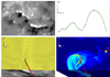 |
Fig. A.2. Detailed presentation of the magnetic flux rope near its peak phase (at time of 16:48 UT on November 7). (a) Two sampled field lines near the axis of the rope. It clearly shows that the winding number of magnetic field lines exceeds three turns. (b) Side view of the field lines shown in the top panel. (c) Vertical cross-section of the MFR whose location is marked by the purple line in panel (a). The arrows show the directions of the transverse field on the slice, as they form spirals centered at the rope’s axis denoted by the red thick line. (d) Same cross section of the axis as in (c) but colored with Tw values, the axis located at the area where the Tw value is the largest. |
All Figures
|
Fig. 1. Basic structure of the studied region seen by SDO/HMI and AIA. Top panel: solar surface with HMI continuum observation. Second panel: vertical component of photospheric magnetic field. Bottom two panels: AIA 171 Å and 304 Å images, respectively. The arrows in the panels mark the location of the filament system. The axes are labeled by the heliographic longitude and latitude from the center of solar disk. |
| In the text | |
|
Fig. 2. Evolution of the GOES soft X-ray flux during 16:00:00 UT to 18:00:00 UT (top panel) and observation of the X1.6 flare in 171 Å (a1–a6), 304 Å (b1–b6), and 1600 Å (c1–c6) bands. The labels T1 to T6 correspond to the time shown in the following panels. The overlaid contours are shown for Bz = 500 G (colored in cyan) and −500 G (pink) in panels a1, b1 and c1. Arrows in panels a1 and b1 indicate the location of the filament. Arrows in panels a2, b2 and c2 point to the circular ribbon of a C7.0 flare. Arrows in panels a3, b3 and c3 indicate the initiation of the X1.6 flare. Arrows in panel b4 show the rising filament with a helical shape. Arrows in panels a5 and b5 point to the eruption of the filament. An animation of this figure is provided online. |
| In the text | |
|
Fig. 3. Evolution of the photospheric magnetic field. The boxed regions labeled with A and B in panel a correspond to the fields of view in panel d and panel e, respectively. Panel f: evolution of the positive magnetic flux in the red box in panel a. An animation of this figure is provided online. |
| In the text | |
|
Fig. 4. Structure and evolution of the MFR and the current density before to after the X1.6 flare. Left column: sampled magnetic field lines shown with different colors for a better view of each field line. Two middle columns: Iso-surface of magnetic twist number Tw = 1 in the x − y plane and in 3D, the structure is false-colored by the value of height z in units of arcsecond (or 720 km). Right column: evolution of the current distribution which is calculated by integration of the current density along the z direction. |
| In the text | |
|
Fig. 5. Evolution of twisted flux of the MFR. Top and middle: evolution of the twist number of the MFR on the cross section whose location is denoted by the red line on the top-middle panel in Fig. 4. Bottom: toroidal magnetic fluxes of the MFR computed on the same cross section, and the fluxes are integrated with only those having Tw ≥ 1. |
| In the text | |
|
Fig. 6. Flare ribbons in 1600 Å (top panel), the squashing degree (Q factor, middle panel), and the twist number distribution (bottom panel) around the PIL before the X1.6 flare peak. |
| In the text | |
|
Fig. 7. Evolution of the twist number Tw, the winding number 𝒯 (including both their largest value and mean value), the decay index, and height of the MFR axis. Parameters in panels b and c are calculated from different positions of the MFR, where panel b corresponds to region A in Fig. 3a (also to the point of intersection between the magenta line and the MFR on the middle-top panel in Fig. 4), panel c corresponds to region B in Fig. 3a (and the point where the red line intersects with the MFR on the middle-top panel in Fig. 4). The height z is in unit of arcsecond (or 720 km). |
| In the text | |
|
Fig. 8. Evolution of the unsigned magnetic flux, the relative helicity, and the energy computed on the AR 12205 region from 00:00 UT to 20:00 UT on 2014 November 7. |
| In the text | |
|
Fig. A.1. Evolution of the CWsin and ⟨|fi|⟩ during 00:00 UT to 20:00 UT on 2014 November 7, shown in the top panel. CWsin and ⟨|fi|⟩ are metrics to measure the quality of force-freeness and divergence-freeness of a NLFFF extrapolation. The black and red dashed lines are average values of the CWsin and ⟨|fi|⟩, respectively. Middle panel: Distributions of the E∇ × B and E∇ ⋅ B during 00:00 UT to 20:00 UT. These two quantities can also be used to measure the force-freeness and divergence-freeness of the extrapolated fields. The black and red dashed lines show the average values of these two metrics, respectively. Bottom panel: Evolution of the free energy. Black and blue lines show the free energy calculated with different ways, the red solid line shows their relative error, and the red dashed line shows the average of the relative error. See the text for details. |
| In the text | |
|
Fig. A.2. Detailed presentation of the magnetic flux rope near its peak phase (at time of 16:48 UT on November 7). (a) Two sampled field lines near the axis of the rope. It clearly shows that the winding number of magnetic field lines exceeds three turns. (b) Side view of the field lines shown in the top panel. (c) Vertical cross-section of the MFR whose location is marked by the purple line in panel (a). The arrows show the directions of the transverse field on the slice, as they form spirals centered at the rope’s axis denoted by the red thick line. (d) Same cross section of the axis as in (c) but colored with Tw values, the axis located at the area where the Tw value is the largest. |
| In the text | |
Current usage metrics show cumulative count of Article Views (full-text article views including HTML views, PDF and ePub downloads, according to the available data) and Abstracts Views on Vision4Press platform.
Data correspond to usage on the plateform after 2015. The current usage metrics is available 48-96 hours after online publication and is updated daily on week days.
Initial download of the metrics may take a while.