| Issue |
A&A
Volume 658, February 2022
|
|
|---|---|---|
| Article Number | A175 | |
| Number of page(s) | 16 | |
| Section | Extragalactic astronomy | |
| DOI | https://doi.org/10.1051/0004-6361/202142059 | |
| Published online | 18 February 2022 | |
XXL-HSC: An updated catalogue of high-redshift (z ≥ 3.5) X-ray AGN in the XMM-XXL northern field
Constraints on the bright end of the soft log N-log S⋆
1
IAASARS, National Observatory of Athens, Ioannou Metaxa and Vasileos Pavlou, 15236 Athens, Greece
e-mail: This email address is being protected from spambots. You need JavaScript enabled to view it.
2
INAF – Osservatorio di Astrofisica e Scienza dello Spazio di Bologna, Via Gobetti 93/3, 40129 Bologna, Italy
3
Astronomical Institute, Tohoku University, 6-3 Aramaki, Aoba-ku, Senda 980-8578, Japan
4
Department of Astronomy, Kyoto University, Kitashirakawa-Oiwake-cho, Sakyo-ku, Kyoto 606-8502, Japan
5
INAF, IASF Milano, via Corti 12, Milano 20133, Italy
6
AIM, CEA, CNRS, Université Paris-Saclay, Université Paris Diderot, Sorbonne Paris Cité, 91191 Gif-sur-Yvette, France
7
Department of Space, Earth and Environment, Chalmers University of Technology, Onsala Space Observatory, 439 92 Onsala, Sweden
8
Research Center for Space and Cosmic Evolution, Ehime University, 2-5 Bunkyo-cho, Matsuyama, Ehime 790-8577, Japan
9
Department of Astronomy, University of Geneva, Ch. d’Écogia 16, 1290 Versoix, Switzerland
10
Academia Sinica Institute of Astronomy and Astrophysics, 11F of Astronomy-Mathematics Building, AS/NTU, No. 1, Section 4, Roosevelt Road, Taipei 10617, Taiwan
11
Universití di Bologna, Dip. di Fisica e Astronomia “A. Righi”, Via P. Gobetti 93/2, 40129 Bologna, Italy
Received:
20
August
2021
Accepted:
8
November
2021
Abstract
X-rays offer a reliable method to identify active galactic nuclei (AGNs). However, in the high-redshift Universe, X-ray AGNs are poorly sampled due to their relatively low space density and the small areas covered by X-ray surveys. In addition to wide-area X-ray surveys, it is important to have deep optical data in order to locate the optical counterparts and determine their redshifts. In this work, we built a high-redshift (z ≥ 3.5) X-ray-selected AGN sample in the XMM-XXL northern field using the most updated [0.5–2 keV] catalogue along with a plethora of new spectroscopic and multi-wavelength catalogues, including the deep optical Subaru Hyper Suprime-Cam (HSC) data, reaching magnitude limits i ∼ 26 mag. We selected all the spectroscopically confirmed AGN and complement this sample with high-redshift candidates that are HSC g- and r-band dropouts. To confirm the dropouts, we derived their photometric redshifts using spectral energy distribution techniques. We obtained a sample of 54 high-z sources (28 with spec-z), the largest in this field so far (almost three times larger than in previous studies), and we estimated the possible contamination and completeness. We calculated the number counts (log N-log S) in different redshift bins and compared our results with previous studies and models. We provide the strongest high-redshift AGN constraints yet at bright fluxes (f0.5 − 2 keV > 10−15 erg s−1 cm−2). The samples of z ≥ 3.5, z ≥ 4, and z ≥ 5 are in agreement with an exponential decline model similar to that witnessed at optical wavelengths. Our work emphasises the importance of using wide-area X-ray surveys with deep optical data to uncover high-redshift AGNs.
Key words: galaxies: active / X-rays: galaxies / methods: data analysis / methods: observational / methods: statistical / early Universe
Based on observations obtained with XMM-Newton, an ESA science mission with instruments and contributions directly funded by ESA member states and NASA.
© ESO 2022
1. Introduction
The majority of massive galaxies in the local Universe host a supermassive black hole (SMBH) in their centre (Magorrian et al. 1998; Kormendy & Kennicutt 2004; Filippenko & Ho 2003; Barth et al. 2004; Greene & Ho 2004, 2007; Dong et al. 2007; Greene et al. 2008). The masses of these SMBHs vary between 105 and 1010 solar masses. The accretion of matter onto the SMBH releases huge amounts of energy across the whole electromagnetic spectrum from the so-called active galactic nucleus (AGN). Even though many studies suggest a correlation between the evolution of galaxies and SMBHs (e.g., Silk & Rees 1998; Granato et al. 2004; Di Matteo et al. 2005; Croton 2006; Hopkins et al. 2006, 2008; Menci et al. 2008), the physical processes behind such a correlation are not fully understood. Thus, a complete AGN sample including a diversity of physical properties (wide range of luminosity, mass, etc.) both at low and high redshifts is essential to better understanding the SMBH evolutionary models and whether SMBHs play a role in the properties of their host galaxies. One of the most efficient ways to detect AGNs is through X-ray emission, since X-rays penetrate the dust and gas surrounding the black hole without being absorbed, thus selecting both low-luminosity and/or moderately obscured black holes. This can be shown in the deepest X-ray fields, including the Chandra Deep Field South (CDFS), where the number density of X-ray-selected AGNs is about 30 000 deg−2 with a median redshift value of z = 1.58 ± 0.05 (Luo et al. 2017). In contrast, the number density of optically selected AGNs is 100 times lower, ∼300 deg−2 (Ross et al. 2013).
However, this picture is reversed at high redshift: the AGN samples are dominated by optically identified quasars compared to the poorly sampled X-ray selected sources. In particular, the number of identified quasars from the first billion years of the Universe has been increasing rapidly over the last years, with tens of thousands of optically selected AGNs with z > 3 and over 200 detected at z > 6 (Bañados et al. 2016; Matsuoka et al. 2019a; Wolf et al. 2021). At higher redshifts (z ≥ 7), only a small number of sources have been detected (Mortlock et al. 2011; Bañados et al. 2018; Wang et al. 2018; Matsuoka et al. 2019b), with the most distant objects being found at z = 7.5 (Bañados et al. 2018; Yang et al. 2020b) and z = 7.642 (Wang et al. 2021). Moreover, the optical surveys find that the normalization of the luminosity function of AGN presents an exponential drop at z ≥ 3 (Masters et al. 2012). This could signpost the continuous creation of new AGNs from a redshift of z ∼ 20 (Volonteri 2010) to redshifts up to z = 2, known as the ‘cosmic noon’ era. Alternatively, the observed drop could be an artefact of reddening associated with the large amounts of gas that are abundant at these early cosmic epochs. On the other hand, just a few X-ray AGNs have been found at these cosmic distances. This is because AGNs are rare and large cosmic volumes or, equivalently, large sky areas are needed to find them. This is possible with the all-sky optical surveys, while X-ray surveys have covered significantly less area for equivalent depths.
In the last years, efforts have been made to compile high-z samples with dedicated X-ray surveys. Vito et al. (2014) identified a total of 141 X-ray sources in the 3 ≤ z ≤ 5.1 redshift range in the 4 Ms Chandra Deep field (CDF) South (Xue et al. 2011), the Chandra-COSMOS (Elvis et al. 2009), and the Subaru/XMM-Newton Deep Survey (SXDS, Furusawa et al. 2008; Ueda et al. 2008) fields. In the SXDS field (which overlaps with the XMM-XXL northern field with an area of 1.14 deg2), there were 30 high-z sources. 20 out of 30 have spectroscopic redshifts from Hiroi et al. (2012). Georgakakis et al. (2015) obtained about 340 X-ray sources in total with both spectroscopic and photometric redshifts in various fields observed with either the Chandra or XMM-Newton X-ray telescopes. In the XMM-XXL northern field, they identified 55 (20) X-ray sources at 3 ≤ z ≤ 5 (z ≥ 3.5) with only spectroscopic redshifts. In the Chandra COSMOS Legacy survey, Marchesi et al. (2016) compiled a sample of 174 sources with 87 of them having available spectroscopic information (3 ≤ z ≤ 5.3).
More recently, Vito et al. (2018) used the deep X-ray observations in the 7Ms CDF-South and 2Ms CDF-North fields to identify102 high-z (3 ≤ z ≤ 6) AGNs, while Khorunzhev et al. (2019) selected a sample of 101 unabsorbed highly luminous quasars (3 ≤ z ≤ 5.1) using the 3XMM-DR4 catalogue (Watson et al. 2009). At higher redshifts (z ≥ 5), in small and deep fields there are only three X-ray sources: two sources in the COSMOS field (Marchesi et al. 2016) with the highest one at z = 5.3 (Capak et al. 2011), and one source in the Chandra Deep Field North (Barger et al. 2003) at z = 5.186. In the larger and shallower XMM-XXL field, Menzel et al. (2016) found a source at z = 5.011, while more recently, with the eROSITA telescope (Predehl et al. 2021) on board the Spectrum-Roentgen-Gamma mission, it was possible to identify one more source at z = 5.46 (Khorunzhev et al. 2021). In addition to the aforementioned studies, there are plenty of known high-z optically selected AGN matched with X-ray catalogues or follow-up X-ray observations (Vito et al. 2016; Medvedev et al. 2020; Wolf et al. 2021). Even though they have not been selected through all-sky or dedicated X-ray surveys, their contribution is crucial to put some lower limits on the AGN space density.
In this work, we focus on selecting a sample of X-ray AGN in the early Universe in the XMM-XXL northern field (Pierre et al. 2016, hereafter XXL Paper I), which has excellent multi-wavelength follow-up observations from the ultraviolet (UV) to the infrared (IR). To achieve this, we built a catalogue of spectroscopically confirmed AGN searching in the publicly available databases, and we complemented it with high-z sources selected through optical colour-colour criteria. We validated the colour-selected candidates through spectroscopic and photometric redshifts that we derive via spectral energy distribution (SED) fitting. Thanks to the Hyper Suprime-Cam (HSC, Miyazaki et al. 2018) data that have deeper photometry, we aimed to select a large sample of z ≥ 3.5 sources and obtain a better constraint on the AGN sky-density distribution for the high-z population, at least for relatively high fluxes. Compared to the previous work of Georgakakis et al. (2015) in the same field, we made use of the most up-to-date X-ray catalogue available that additionally includes the XMM-Newton observations occurred after 2012, thus increasing the total surveyed area by ∼40%. Furthermore, besides the new spectroscopic data from the Sloan Digital Sky Survey (SDSS) IV and other surveys, we derive the photometric redshifts of all the colour-selected candidates, therefore increasing the number of high-z sources. An additional advancement is that the HSC data covering the area are much deeper than the SDSS or the Canada-France-Hawaii Telescope Legacy surveys, reaching magnitudes down to r ≃ 26 mag (Aihara et al. 2019). These depths are critical for the identification of AGN and, especially, the most obscured AGN where the nucleus is covered by veils of dust and gas and only the galaxy remains visible. To this end, we will be able to put much stronger constraints on the AGN sky density and compare the theoretical population synthesis models at this redshift regime for bright fluxes for the first time.
The data used in this work are presented in Sect. 2. These include the X-ray catalogue and the multi-wavelength information along with the spectroscopic catalogues. In Sect. 3, we present the high-z sample selected through optical spectroscopy and the Lyman Break selection criteria. We also derived the photometric redshifts using SED fitting, and we considered the contamination and reliability of our sample. In Sect. 4, we calculate the cumulative numbers in different redshift bins and constrain the bright flux of the log N-log S relation. In Sect. 5, we discuss and summarise the results. Throughout the paper, we assume a ΛCDM cosmology with H0 = 70 km s−1 Mpc−1, ΩM = 0.3, and ΩΛ = 0.7.
2. Data
In this section, we describe the data used in this work to select high-z X-ray AGN in the XMM-XXL northern field. We used the X-ray catalogue that was derived from the latest XMM-XXL pipeline and the deep HSC data in order to build the broad-band optical colours. Moreover, we used all the available spectroscopic data covering the field. In parallel and in addition to HSC data, for the SED construction we used the ancillary data accompanying the X-ray catalogue that contains rich multi-wavelength data from the UV to the mid-IR bands. The SEDs were used to estimate the photometric redshifts (photo-z) for those objects lacking spectroscopic redshift (spec-z). Below, we give a brief description of the aforementioned data and their surveys.
2.1. XMM-XXL northern catalogue
The XMM-XXL survey (XXL Paper I) is the largest XMM-Newton programme approved (> 6 Ms) surveying two extragalactic sky regions of approximately equal size. This totals ∼50 deg2 with a median exposure time of about 10 ks per XMM-Newton pointing and a depth (at 3σ) of ∼5 × 10⁻¹⁵ erg s−1 cm−2 in the 0.5–2 keV X-ray band. The X-ray data used in this study rely on an internal release obtained with the V4.2 XXL pipeline. The reader should be aware that the V4.2 version is expected to be superseded by the final catalogue, V4.3. Compared to the previous version V3, where the XMM observations were treated individually, the V4 version of the pipeline processes all the co-added observations together into 1 × 1 deg2 mosaics, which enhances the detection sensitivity at any position. Furthermore, this version of the catalogue includes observations performed after 2012. These include a total of 1.3 Ms observations with a median PN exposure time of ∼46 ks covering the XMM-Spitzer Extragalactic Representative Volume Survey (XMM-SERVS) field with an area of 5.3 deg2 (Chen et al. 2018). In the analysis, we used the data from the equatorial sub-region of the field (4XMM-XXL-Northern; 4XXL-N) centred at RA ∼ 2h16m, Dec ∼ −4°52′, which covers an area of about 25 deg2 and contains 15547 X-ray sources (Chiappetti et al. 2018, hereafter XXL Paper XXVII). Restricting our sample to sources detected in the soft band, we ended up with 13742 X-ray sources. In the considered redshift range (z ≥ 3.5), the [0.5–2] keV energy band corresponds to rest-frame energies greater than [2.25–9] keV.
The 4XXL-N was accompanied by a multi-wavelength catalogue covering the spectrum from the UV up to the mid-IR bands. In particular, it includes UV data from the GR6/7 release of the Galaxy Evolution Explorer survey (GALEX, Bianchi et al. 2014) and optical data from the T0007 data release (Hudelot et al. 2012) of the Canada-France-Hawaii Telescope Legacy Survey (CFHTLS) and the 10th data release of the Sloan Digital Sky Survey (SDSS, Ahn et al. 2014). In the near-IR, the XXL-N field was covered by three European Southern Observatory (ESO) surveys with the Visible and Infrared Survey Telescope for Astronomy (VISTA, Emerson et al. 2006): the VISTA Hemisphere Survey (VHS, McMahon et al. 2013), the VISTA Kilo-degree Infrared Galaxy Survey (VIKING, Edge et al. 2013), and the VISTA Deep Extragalactic Observations survey (VIDEO, Jarvis et al. 2013). Additionally, the multi-wavelength catalogue includes near-IR data from the UKIRT Infrared Deep Sky Survey (UKIDSS, Dye et al. 2006) and the WIRcam camera on CFHT in the Ks band (Moutard et al. 2016). Finally, the catalogue was complemented with mid-IR photometry from the ALLWISE data release of the Wide-field Infrared Survey Explorer (WISE, Wright et al. 2010) all-sky survey and the observation from the Infrared Array Camera (IRAC, Fazio et al. 2004) on board the Spitzer Space Telescope (Werner et al. 2004). The X-ray sources in the 4XXL-N were assigned a counterpart from this catalogue if there were detections in at least one band. The source matching was performed using the likelihood ratio estimator (Sutherland & Saunders 1992). All of the X-ray sources were matched with existing catalogues. In particular, a counterpart was found for about 86% of the sources in the optical, followed by 9.2% and 4.4% in near-IR and mid-IR or UV datasets, respectively. More details regarding the cross-matching techniques and the photometric data can be found in Fotopoulou et al. (2016, hereafter XXL paper VI) and XXL Paper XXVII.
2.2. HSC-PDR2 catalogue
We made use of the optical imaging data obtained with the Subaru Hyper-Suprime Camera (HSC), which is much deeper (i ∼ 26 mag) compared to the SDSS and CFHT optical surveys with magnitude limits (at 5σ) of i ∼ 21.3 mag and i ∼ 24.5 mag, respectively. More specifically, we used the second public data release (HSC-PDR2, Aihara et al. 2019) of the Hyper Suprime-Cam Subaru Strategic Program (HSC-SSP, Aihara et al. 2018). The full description of the HSC-SSP survey can be found in Aihara et al. (2019). Although the HSC-PDR2 data are taken in three layers with different areas and depths (Wide, Deep, and UltraDeep), we only used the wide field layer in this study. The overlapping area between 4XXL-N and HSC-PDR2 is approximately ∼24 sq. degrees, while the HSC-PDR2 5σ sensitivity limits in the field reach mag 26.6, 26.2, 26.2, 25.3, and 24.5 in the AB magnitude system for the g, r, i, z, and y bands, respectively.
In order to get a clean photometry, we followed the procedure described on the HSC-PDR2 website. Thus, we only selected the primary sources and excluded those flagged with bad pixels, saturation, or interpolation, hit by cosmic rays or located at the edges of the detector. Furthermore, we used the PDR2 masks centred around bright stars obtained by the Gaia DR2 catalogue. About 20% of the sources were masked. To separate point-like and extended sources, we made use of the moments (Akiyama et al. 2018) in the i-band, because the i-band image has the highest image quality among the five bands in the HSC-SSP survey data (Aihara et al. 2019). We used the PSF magnitudes for the point-like sources and the CMODEL magnitudes for the extended ones, which were estimated by fitting the PSF model and a two-component model (Abazajian et al. 2004; Bosch et al. 2018), respectively.
2.3. 4XXL-HSC sample
The common area between the HSC data (excluding the masked areas) and the 4XXL-N is about 20 deg2. This area includes 10998/13742 (∼80%) X-ray sources detected in the soft band. The HSC catalogue was cross-matched with the list of the X-ray sources using the coordinates of the ancillary data in a similar way to XXL paper VI (Sect. 4.1). In particular, we used a simple positional cross-matching method with a search radius depending on the data matched. Firstly, we cross-matched the HSC sources with the optical coordinates of the multi-wavelength catalogue with a radius of 1″. For those X-ray sources without an optical counterpart, we used the coordinates of the near-IR bands (1″) followed by the coordinates of the mid-IR and UV bands (2″). We ended up with 9689/10998 (∼88%) X-ray sources with HSC counterparts (hereafter 4XXL-HSC). Out of these, 7169 and 2520 sources are optically extended and point like, respectively.
In Fig. 1, we show the 4XXL-HSC magnitude distributions in the i-band from the HSC data along with the SDSS and CFHT data for comparison. Including the HSC data, we go almost a magnitude deeper compared to the CFHT photometry, and we have a higher number of optical counterparts. Moreover, the uncertainties of the HSC data are much lower for the fainter objects; thus, our colour-selection criteria and photometric redshift estimations will be more precise.
 |
Fig. 1. Magnitude distributions of the 4XXL-HSC sources for the CFHTLS (filled gray), SDSS (solid blue), and HSC (dashed red) i bands. |
2.4. Spectroscopic catalogues
In the XMM-XXL northern field, there are plenty of spectroscopic surveys targeting extragalactic sources, both galaxies and AGN. Most of them target sources that were pre-selected in the UV or optical wavelengths, while there are some dedicated only to X-ray-selected sources. In our analysis, we used the spectroscopic catalogues of X-ray-selected AGN by Menzel et al. (2016) and Hiroi et al. (2012). Moreover, we used the spectroscopic data gathered by the HSC team. In particular, they include the PRIsm MUlti-object Survey (PRIMUS Coil et al. 2011; Cool et al. 2013) in the sub-region XMM-LSS (∼2.88 deg2) of the XXL-N, the Galaxy And Mass Assembly (GAMA, Liske et al. 2015), the VIMOS VLT Deep Survey (VVDS, Le Fèvre et al. 2013), and the VIMOS Public Extragalactic Survey (VIPERS, Garilli et al. 2014). Also, in this database the DR12 (Alam et al. 2015) and DR14 (Pâris et al. 2018) of the SDSS are included. Additionally, we used the latest data release (SDSS-DR16, Ahumada et al. 2020) that is the fourth release of the Sloan Digital Sky Survey IV. The spectroscopic information provided by the HSC team was already associated with the photometric catalogue of the sources. For the remaining datasets, the spectroscopic catalogues were matched to the optical positions in our sample with a radius of 1″. For all the sources, we selected high-quality flags that correspond to a probability of 90% or higher that that redshift is the true one.
3. Sample selection
In this section, we present the final sample of the high-z sources in the XXL-N field. We list the confirmed high-z sources found in the publicly available spectroscopic catalogues and also the colour-selected AGN. To account for any contamination by low-z interlopers, we used the spectroscopic redshifts, and for the remaining sources we estimated the photo-z with the X-CIGALE algorithm (Yang et al. 2020a). Furthermore, we used the X-ray-to-optical flux ratio as an additional criterion to account for brown dwarf contamination.
3.1. Spectroscopic redshifts
Using the spectroscopic catalogues mentioned in Sect. 2.4, we initially selected all the X-ray sources with z ≥ 3.5. In particular, from the latest data release of SDSS (DR16; Ahumada et al. 2020), we select 37 objects. Also, we made use of the spectroscopic information provided by the HSC PDR2 database and selected 27 sources at high redshift and assigned with a secure flag. Furthermore, we included 19 and 8 sources with spectroscopic redshifts found in Menzel et al. (2016) and Hiroi et al. (2012), respectively. It is worth mentioning that there are two sources with spectroscopic redshift in Menzel et al. (2016) without X-ray counterparts in the 4XXL catalogue. This is probably due to different source detection algorithms or background estimations used. The first one lies at z = 3.67, while the second one is the most distant X-ray source in their catalogue at z = 5.011. Both sources are broad-line AGNs of type 1, according to their optical spectra (Liu et al. 2016), and do not show strong absorption in the X-ray regime (log NH < 21.3). These sources were not taken into consideration in this study. The discrepancies between the two X-ray catalogues are beyond the scope of this study and will not be discussed further.
In total, taking into account the overlaps within these catalogues, we yielded 45 sources at high redshifts. Even though all these sources have secure measurements according to the flags provided, we visually inspected all the individual spectra for probable outliers or low-quality sources. We excluded nine sources, since their spectra were too noisy, resulting in 36 spec-z sources. Out of those, 28 spec-z sources fell in good regions (outside of the HSC masked areas). 22 out of 28 (79%) are point-like sources, while six sources appear extended in the HSC optical images.
3.2. High-z dropout candidates
We complement the spectroscopically confirmed sources by using the Lyman Break colour selection method for the 4XXL-HSC sample. The Lyman Break technique (Steidel et al. 1996, 1999; Giavalisco 2002) has been widely used to select high-z sources using UV, optical, or IR filters. In this work, we used a set of colours and criteria similar to Ono et al. (2018) for both point-like and extended sources in order to select candidates at z ∼ 4 − 7. Sources at z = 4, 5, 6, and 7 are expected to be selected by the gri, riz, izy, and zy colours, respectively. In brief, we applied the following criteria to the 4XXL-HSC sample:
For g-dropouts (z ∼ 4):
 (1)
(1)
 (2)
(2)
 (3)
(3)
For r-dropouts (z ∼ 5):
 (4)
(4)
 (5)
(5)
 (6)
(6)
For i-dropouts (z ∼ 6):
 (7)
(7)
 (8)
(8)
 (9)
(9)
 (10)
(10)
For z-dropouts (z ∼ 7):
 (11)
(11)
These colours returned 69 high-z candidates, 68 g-dropouts, and 1 r dropout in total. We did not have any i or z dropouts. Out of these, there are 27 point-like and 42 extended sources. Figure 2 shows the colour-colour plots for g- and r-band dropouts. The orange points inside the wedges (dashed lines) represent the dropout sources in each selection method, while the grey points represent all 4XXL-HSC sources. There are some sources inside the wedges not selected as high-z candidates, since they did not meet the signal-to-noise detection threshold criteria mentioned above.
 |
Fig. 2. (g–r, r–i) and (r–i, i–z) colour-colour plots (from top to bottom). The black lines indicate the selection criteria defined by Ono et al. (2018). The small grey points indicate the full 4XXL-HSC sample, and the orange squares represent the high-z candidates. We over-plot the specz-z sample (asterisks) colour-coded with the redshift, while we highlight the dropouts with zphot ≥ 3.5 in blue. |
Finally, we constructed, in addition to the above criteria, a high-z sample on the basis of the broad-band colours described in Akiyama et al. (2018). The latter criteria that were optimised only for the point-like sources and especially for the high-z quasars rely on the different colours used (g–r vs. r–z) compared to the classic g–r vs. r–i. Furthermore, since Akiyama et al. (2018) were interested in the redshift range of z ∼ 3.5–4.5, we relaxed their criteria, thus including sources with higher redshifts. Therefore, besides their original criteria (case A), we included the area with g–r colour greater than 1.5, not limiting us to sources up to z = 4.5 (case B), and also a second area where there are quasars with much higher redshifts (case C). These additional criteria were based on the spectroscopic information of known quasars and stars as shown in Akiyama et al. (2018, see their Fig. 2). Below, we summarise these optimised criteria.
Case A:
 (12)
(12)
 (13)
(13)
 (14)
(14)
Case B:
 (15)
(15)
 (16)
(16)
 (17)
(17)
Case C:
 (18)
(18)
 (19)
(19)
In Fig. 3, we plot the selected dropout sources in the g − r versus r − z colour spaces. By applying these criteria, we were able to identify 33, 14, and 12 high-z candidates in cases A, B, and C, respectively, resulting in 59 sources in total. Concerning the overlap between sources derived by the Ono et al. (2018) and Akiyama et al. (2018) methods, the latter recovered all the point-like sources, but additionally selected 32 sources. Thus, the addition of the extra criterion was critical to select a more complete high-z sample. In total, using both selection criteria of the aforementioned studies, we were able to build a sample of 101 unique high-z candidates.
 |
Fig. 3. (g − r, r − z) colour-colour plot. The black lines indicate the selection criteria defined by Akiyama et al. (2018), including the complementary criteria from this work. The small grey points indicate the point-like sources in the 4XXL-HSC sample, while the orange squares represent the high-z candidates in Cases A, B, and C (see text for details). We over-plot the specz-z sample (asterisks) colour-coded with the redshift, while we highlight the dropouts with zphot ≥ 3.5 in blue. |
The sources derived with the broad-band selection methods are expected to be contaminated by a population of low redshift interlopers and also by brown dwarfs. Concerning the low-z interlopers, we used the spectroscopic information of the sources, if available, and for the remainder we derived the photometric redshift stated in the next section. Also, in our case the contamination from the stellar objects is expected to be negligible, since we used X-ray-selected sources well fitted with AGN templates (Sect. 3.3.1). In Sect. 3.4, we address both these issues in detail.
3.3. Photometric redshifts
Out of the final 101 dropouts, 31 have a counterpart in one of the spectroscopic catalogues. Out of these, 21 (68%) sources have zspec ≥ 3.5, while 10 (32%) sources have lower redshifts. The vast majority of the latter are located outside the Ono et al. (2018) wedges in all colour diagrams, while they are all marginal to those of Akiyama et al. (2018). For the remaining 70 dropouts lacking spectroscopic information, we derive the photometric redshifts using all the available data from UV to mid-IR wavelengths. In this section, we present the method used to derive the photometric redshifts and the different statistical approaches used to calculate its accuracy and reliability.
3.3.1. SED fitting
We performed a multi-component SED fitting with the X-CIGALE algorithm to estimate the photometric redshifts. X-CIGALE is the latest version of the Code Investigating GALaxy Emission (CIGALE, Noll et al. 2009; Ciesla et al. 2015; Boquien et al. 2019) and has recently been used for redshift estimations in the early Universe with high precision (Barrufet et al. 2020; Toba et al. 2020; Shi et al. 2021). For example, Shi et al. (2021) found a catastrophic failure ratio of 10% with normalised uncertainty σNMAD = 0.08. The X-CIGALE code fits the observational multi-wavelength data with a grid of theoretical models and returns the best-fit values for the physical parameters. The results are based on the energy balance, that is, the energy absorbed by dust in the UV and the optical is re-emitted after heating at longer wavelengths, such as the mid-IR and far-IR.
For the SED fitting, we used all the available data covering the wavelength range from the UV light up to mid-IR bands. In our analysis, we used redshift values between 0.0 and 7.0 with a step of Δz = 0.05, while we built a grid of models including different stellar populations, dust attenuation properties, dust emission, star formation history, and AGN emission. With this configuration, for each source we fitted the observational data to more than 350 million models. The models and the parameter space covered by the SED components are described below.
For the stellar population, we used the synthesis models of Bruzual & Charlot (2003) with the Initial Mass Function (IMF) by Salpeter (1955) and a constant solar metallicity at Z = 0.02. A constant metallicity does not affect significantly the shape of the SEDs (Pouliasis et al. 2020, and references therein). For the attenuation originated in the absorption and scatter of the stellar and nebular emission by interstellar dust, we used the Calzetti et al. (2000) attenuation law. The emission by dust in the IR regime was modelled by the Draine et al. (2014) templates, an updated version of the Draine & Li (2007) models that allowed us to include higher dust temperatures. The main parameters that describe them are the mass of the PAH population, qPAH, and the dust temperature, which is expressed with the minimum radiation field, Umin (Aniano et al. 2012).
The AGN templates used in our analysis are based on the realistic clumpy torus model presented in (Stalevski et al. 2012, 2016; SKIRTOR). SKIRTOR assumes a clumpy two-phase torus model that considers an anisotropic, but constant, disk emission. More details about the SKIRTOR implementation in X-CIGALE can be found in Yang et al. (2020a). The parameter space for this module followed the description in Yang et al. (2020a) and Mountrichas et al. (2021). Moreover, with X-CIGALE it is possible to include the polar dust extinction (Mountrichas et al. 2021; Toba et al. 2021). Finally, for the star formation history (SFH), we used a double-exponentially decreasing model (2τ-dec) with different e-folding times.
Table 1 lists the models and the parameter space used in the SED fitting procedure. We removed seven sources (1 has spectroscopic redshift) with very high reduced χ2 values,  (Mountrichas et al. 2021), from the SED fitting process. These were mainly very faint sources detected in only a few bands and/or located in high source density areas. Finally, for each source, we obtained the full probability density function of the redshift, PDF(z). In Fig. 4, we give an example of the SED and the PDF(z) of the source with ID = J021613.8-040823 and zspec = 3.522. The peak of the PDF(z) for this source is zpeak = 3.55.
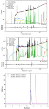 |
Fig. 4. Examples of SED fits of a spec-z source (ID=J021613.8-040823, upper) and a photo-z source (ID=J020245.0-044223, middle). The dust emission is plotted in red, the AGN component in orange, the attenuated (unattenuated) stellar component is shown by the solid yellow (blue) (dashed) line, while the green lines show the nebular emission. The total flux is represented in black. Below the SEDs, we plot the relative residual fluxes versus the wavelength. Lower panel: The probability density function of redshift, PDF(z), of the sources with a peak at zpeak = 3.55, and the sources with a peak at zpeak = 4.25, respectively. The vertical line shows the spectroscopic redshift of J021613.8-040823 at zspec = 3.522. |
Models and their parameter space used by X-CIGALE for the SED fitting of the colour-selected high-z sources.
3.3.2. Photo-z performance
The photometric redshift accuracy for the high-z candidates was investigated using the dropout sample of 30 sources with available spectroscopic information and low  values. The scatter between the photometric and spectroscopic redshifts is usually estimated using the traditional statistical indicators: the normalised median absolute deviation σNMAD (Hoaglin et al. 1983; Salvato et al. 2009; Ruiz et al. 2018) and the percentage of the catastrophic outliers η (Ilbert et al. 2006; Laigle et al. 2016), defined as follows:
 (20)
(20)
 (21)
(21)
where Δz = zphot − zspec, Ntotal is the total number of sources and Noutliers is the number of the outliers. To be consistent with previous works in the literature, we define an object as an outlier if it has |Δz|/(1 + zspec) > 0.15. We obtained the values η = 26.7% and σNMAD = 0.08 for the whole sample, but when considering only spec-z sources at high redshift (z ≥ 3.5), the situation significantly improves, with η = 9.5% and σNMAD = 0.05. In Fig. 5, we show the photo-z peak values (red crosses) as functions of the spec-z. There are two extreme outliers in the high-z regime, ID: J021952.8-055958 and J021727.6-051718, with spec-z equal to 3.86 and 3.97, respectively. We show the PDF(z) of these sources in Fig. 6 with dashed lines. Even though, they are spectroscopically confirmed high-z sources, the nominal value of the redshift is at z ≃ 0.5, while there is a secondary peak around the true value.
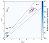 |
Fig. 5. Photometric versus spectroscopic redshifts for the 30 dropouts that have available spec-z information. The dotted lines represent the limits of the catastrophic outliers. The points are colour-coded with the relative redshift probability. Red crosses represent the peaks of the PDFs. A and B indicate the two extremes outliers, ID: J021727.6-051718 and J021952.8-055958, respectively. |
A caveat of the classic scatter estimation method is that it only considers the PDF’s most likely values (i.e. the mode) and not the PDF(z) as a whole. In order to correctly estimate the systematic biases of the scatter and the percentage of outliers using all the information contained in the PDF(z) obtained with X-CIGALE, we followed a more updated and refined interpretation of the biases proposed by Buchner et al. (Appendix B, 2015). The idea is to find the  and
and  values that maximise the likelihood that the true redshift of the source (spec-z) is given by the full PDF(z). The likelihood is given by a modified version of the PDF(z), with a term that is the broadening of the PDF(z) due to the scatter (convolution with a Gaussian with zero mean and standard deviation,
  ), plus a constant term due to the probability of it being a catastrophic outlier:
 (22)
(22)
Then, the total likelihood to maximise is the product of the SYSPDF(z) value for the corresponding spec-z of each source:
 (23)
(23)
Using a simple numerical minimisation method for the likelihood, we find  = 12.6% and
  = 0.04. However, for a better estimation of the parameters, we used the UltraNest code (Buchner 2021), a Bayesian posterior sampling method based on nested sampling (Skilling 2004, 2009). We assumed for both
  and
and  uniform Jeffreys priors (i.e. a uniform prior in the logarithmic space) with limits (1e−4,1.0) and (1e−3,1.0), respectively. This way, we may have a complete characterisation with the posterior probability distribution of the parameters. To this end, the systematics of our sample are given by
  and
and  .
.
In Fig. 5, we show the comparison between the photo-z and spec-z. In addition to the most likely values (peak of the PDF, red crosses), we provide the full PDF(z). The grid is colour-coded with the relative redshift probability in each bin. We incorporate these systematic errors in the PDF(z) of our sample using Eq. (22). In Fig. 6, we show the individual corrected PDF(z) for two spectroscopically confirmed high-z sources, while in Fig. 7, we show the redshift distribution of the dropout-selected objects with spec-z and photo-z. In particular, the grey histogram represents the distribution of the peaks of the PDF(z), while the blue solid line is the distribution when we sum the SYSPDF(z) of all sources together (corrected for  and
and  ). For comparison, we also show the sum of the PDF(z) with red dashed line. In general, the two distributions (sum of PDF or SYSPDF and the simple source counts) agree with each other, showing that the majority of the sources have a PDF(z) with a single, narrow peak. In the same plot, we show the distribution of the dropouts with confirmed redshifts.
 |
Fig. 6. PDF(z) of two sources, J021952.8-055958 (blue dashed) and J021727.6-051718 (green dashed), with spec-z 3.86 and 3.97 (vertical dotted lines), respectively. The corrected PDF(z) for systematics, SYSPDF(z), are shown with solid lines. |
 |
Fig. 7. Redshift distribution for the 63 photo-z sources. The filled grey histogram presents the photo-z peak values, while the red dashed (blue solid) line shows the distribution when summing the PDF (SYSPDF) of all sources. For reference, we plot the 30 dropouts with spectroscopic redshift (black histogram). |
3.4. Purity and completeness
In order to estimate the reliability and completeness of the Lyman Break technique, we used the spectroscopically confirmed high-z AGN sample. In the 4XXL-HSC area, we selected 28 confirmed high-z sources (Sect. 3.1). In Figs. 2 and 3, we show the positions of spec-z sources in the colour-colour diagrams. The dropout selection criteria recovered 21 out of 28 (75%) sources. Out of the non-selected sources, two lie very close to the wedges, while one source lies inside the wedges but did not meet the criteria concerning the signal-to-noise ratio. The spectra of the remaining sources show that strong emission lines fall between the windows of the photometric filters and affect the spectral colours.
Furthermore, the different colour-colour selection criteria allow contaminants, such as low-z galaxies and/or brown dwarfs, in the high-z sample. Concerning the stellar contamination, besides the X-ray emission that is a strong signature of AGN, we used the X-ray (FX) to optical flux (Fopt) ratio, FX/Fopt (Maccacaro et al. 1988; Barger et al. 2003; Hornschemeier et al. 2003). This relation is a well-known method used to verify that a given object is an AGN, and it has been used in many studies (e.g., Pouliasis et al. 2019). The typical AGN population lies in the area between log(FX/Fopt) = ± 1 with some spectroscopically confirmed AGNs extended up to log(FX/Fopt) = ± 2. Conversely, stars have low X-ray emission relatively to their optical emission (log(FX/Fopt)≤ − 2), and thus they can be discerned very well from the AGNs that are powerful X-ray emitters. In Fig. 8, we plot the X-ray flux (0.5–2 keV) versus the optical magnitude (i-band) of all the colour-colour selected sources with detections in the soft band. The sources with spectroscopic redshifts cover the area of the bright optically end, while the photo-z sources are fainter in the optical but have similar X-ray flux to the latter.
 |
Fig. 8. Soft (0.5–2 keV) X-ray flux versus optical (i-band) magnitude for the dropouts (grey points). Blue squares represent the sources with photo-z (peak) higher than 3.5. The green triangles (red circles) show the sources with zspec ≥ 3.5 (zspec < 3.5). The solid line indicates the log(FX/Fopt) = 0, and the dashed lines from left to right correspond to log(FX/Fopt) = − 2, −1, +1, respectively. The X-ray fluxes are plotted in logarithmic scale and given in units of ergs cm−2 s−1, while the optical magnitudes are in the AB system. The dashed and dotted contours show the high-z samples of Georgakakis et al. (2015) and Marchesi et al. (2016), respectively. |
The bulk of our high-z candidates are distributed over the whole area within FX/Fopt = ±2, which is indicative of their AGN nature. However, there are some rare cases of flaring ultra-cool dwarfs (De Luca et al. 2020) of type ∼M7-8 up to L1 with typical luminosity values of ∼1030 erg s−1 that could reach very high X-ray-to-optical ratios (log(LX/Lopt)≃ − 1) and contaminate our sample. In our case, however, all the SEDs of the final 63 photo-z sources are well fitted by AGN templates: 98% and 60% of the sources have  and
and  , respectively. Furthermore, ∼55% of this sample is composed of extended sources. In Fig. 8, we also plot the high-z AGNs selected by Georgakakis et al. (XXL – smaller and shallower area than in our case, 2015) and Marchesi et al. (COSMOS – narrow and deep field, 2016) for reference. Our sources cover the regions of both these surveys. This is because, in our analysis, we used new X-ray observations in the XMM-XXL field in addition to the deep HSC data. We were thus able to push the X-ray and optical limits similarly to COSMOS field.
Concerning the low-redshift interlopers, Ono et al. (2018) criteria include requirements in the detection threshold – high signal-to-noise ratio for the redder bands and non-detections in bluer bands – to avoid low-z contaminants as much as possible. Even though in applying these criteria they estimated the fraction of low-z interlopers to be less than 10% for faint (> 24 mag) sources and about 40% for brighter sources in the redshift range around z = 4. When studying only point-like sources, Akiyama et al. (2018) found that the expected contamination comes from compact objects at magnitudes > 23 in the i band with a fraction of ∼30%. In our study, we used the spectroscopic and photometric redshifts to estimate the possible contamination of the dropout selection method. Using the spectroscopic sample (31 sources), 68% have zspec > 3.5, while 32% with lower redshifts contaminate our sample with an average redshift zmean = 0.77. For the remaining sources (63) lacking spectroscopic redshifts, we used the photo-z estimations. There are 37/63 (∼58.7%) with z < 3.5. This is expected, if we take into account that at fainter magnitudes the colour selection becomes less reliable because of increased uncertainties.
3.5. High-z sample – summary
Table 2 summarises the numbers of high-z sources in different redshift bins selected through our analysis. In particular, there are a total of 28 sources with secure spectroscopic redshift at z ≥ 3.5. Nine sources have z ≥ 4, and one source has a redshift greater than five (ID= J020736.7-04254 with zspec = 5.35). Furthermore, we selected 63 sources through colours that have no available spectra. Using the derived SYSPDF of the photometric redshifts, we were able to select an additional 26 sources with PDF peaks zpeak ≥ 3.5. However, by considering the information contained in the full SYSPDF(z) of all the 63 sources, we were able to include in our analysis cases with lower probabilities being at high z. The spec-z sources were assigned with weight equal to one. In this case, the effective number counts above redshift 3.5, 4, and 5 are 55.3, 23.9, and 5.6, respectively. Figure 9 presents the redshift distribution of the final sources. This includes the spec-z sample (black histogram) and the sum of the SYSPDF(z) of all 63 photo-z sources (blue line). Table A.1 in the appendix lists all 91 X-ray sources (28 spec-z and 63 photo-z) that we used for the log N-log S estimations in the next section.
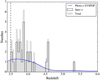 |
Fig. 9. Redshift distribution of our final high-z sample (grey filled). We highlight the spec-z and the photo-z (sum of the SYSPDF). The vertical line indicate the redshift limit in our analysis (z ≥ 3.5). |
Number of sources in different redshift bins.
We compared our final high-z sample with previous studies in the XMM-XXL northern field. Among the spectroscopic catalogue of Menzel et al. (2016), there are 55 z ≥ 3.0 sources used for the luminosity function calculation in Georgakakis et al. (2015). In their sample, there are 20 sources at z ≥ 3.5. Two sources with z = 3.67 and z = 5.011 do not have counterparts in the 4XMM-XXL catalogue. From the remainder, 15 out of 18 sources were also selected through colours in our analysis. In our case, since we used the most updated X-ray observations that cover an area that is ∼40% and expanded our analysis to photo-z sources, we were able to select almost three times more high-z sources. Moreover, using the most recent SDSS spectroscopy, our sample includes 1.5 times more high-z sources with spectroscopic redshift. Out of the 141 sources detected by Vito et al. (2014) in various fields, 30 sources lie inside the SXDS field (Ueda et al. 2008), 12 of which have z ≥ 3.5. Two X-ray sources with photometric redshift (z = 3.6 and z = 4.09) in their study do not have a counterpart in the 4XMM-XXL catalogue. Out of the remainder, we included all eight sources with spec-z in our sample – five of the them are dropouts. Finally, Khorunzhev et al. (2019) compiled a catalogue of high-luminous, high-z sources (LX, 2 − 10 keV > 10−15 erg s−1) from the XMM-Newton serendipitous survey catalogue. Among these sources, seven fall inside the 4XXL-N field and have a 4XXL counterpart. In our analysis, we included five out of seven sources with zspec ≥ 3.5.
4. Number counts
The cumulative number counts (the so-called log N-log S relation) is a very handy tool used to describe and constrain the properties of the different AGN populations and test the theoretical assumptions concerning the evolution and the properties of the Universe. Taking into account the advantage of the large number of the high-z sources selected through our analysis, we were able to derive the number counts in the redshift bins z ≥ 3.5, z ≥ 4, and z ≥ 5 in the soft 0.5–2 keV X-ray band. In the redshift bin z ≥ 6, the main contribution in the number counts was originated from the scatter and the probability of being a catastrophic outlier components. Thus, we did not include this redshift bin in our results. In Fig. 10, we show the flux distribution in the soft 0.5–2 keV band for the 4XXL catalogue. We also over-plot the distribution of the high-z sample (spec-z and photo-z) that ranges between 5 × 10⁻¹⁶ and 3 × 10⁻¹⁴ erg s−1cm−2, which is more than one order of magnitude. To calculate the integral form of the number count distribution we followed the traditional method defined as follows:
 (24)
(24)
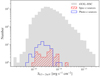 |
Fig. 10. Flux distribution in the soft (0.5–2 keV) band for all sources in the 4XXL-HSC catalogue (gray filled). The red dashed (blue solid) histogram represents the high-z sample with spectroscopic (photometric) redshift estimation. |
where N is the surface number density of sources with S > Sj, and Sj is the lower edge of the bin. Ωi is the solid angle in which a source with flux Si could have been detected and M is the number of sources with S > Sj. We further included the weight, which is the integral of the SYSPDF(z) above a given redshift:
 (25)
(25)
with z0 the minimum redshift in each bin. wi is the probability that the object lies above redshift z ≥ z0. For spec-z sources, we fixed this value to one.
We calculated the uncertainties using the bootstrap method. Thus, we randomly generated 10 000 realisations of the high-z sample with the same size allowing for repetitions. Next, we assigned a random redshift value to each source following its SYSPDF(z). For sources with spec z, we kept the spec-z value. At the end, for each list we calculated the log N-log S and the average 1σ and 2σ values from all iterations. We used the area curve derived from the 4XXL catalogue in the soft band. As a sanity check, we calculated the log N-log S for the whole 4XXL catalogue. In Fig. 11, we show the cumulative numbers derived from this work compared to previous studies. In particular, we overplot the log N-log S trend derived in XXL Paper XXVII with the 3XXL catalogue by Luo et al. (2017) in the 7 Ms CDFS and by LaMassa et al. (2016) in the Stripe 82X field. The number counts agree very well with the aforementioned studies, indicating that the area curve produced for the 4XXL sample is correct.
 |
Fig. 11. Cumulative number counts for the whole 4XXL catalogue are presented with the shaded area highlighting the 1-σ error in the soft 0.5–2 keV band. For reference, we over-plot the number counts derived by XXL Paper XXVII, Luo et al. (2017) and LaMassa et al. (2016). |
In order to use the area curve derived from the full 4XXL catalogue, we had to correct for the incompleteness due to the optically selection effects that appear in the 4XXL-HSC catalogue. In particular, as reported in Sect. 2.3, ∼88% of the X-ray sources are matched with an optical counterpart. The incompleteness arises from the quality of the HSC data. The majority of non-selected sources are affected by saturation, bad pixels, bright-object neighbouring or near-edge issues that we initially discarded from our sample. We may estimate the fraction of the X-ray sources that have a good HSC match for each of the log N-log S bins and correct for this incompleteness by adding an additional weight in Eq. (24). Furthermore, the 4XXL-HSC area is much smaller compared to the total area covered by the 4XXL data, because the HSC data do not cover the full area of 4XXL and also because we excluded the HSC masked areas due to bright stars. We corrected this by normalising the number counts to the total area. Finally, we examined if the dropout sources excluded from our sample due to their high reduced χ2 values could affect the number counts. Out of seven sources, one is spectroscopically confirmed at zspec = 1.24 and one is found in the outskirts of the nearby galaxy 2MASX J02210771-0459574 (z = 0.13) with biased photometry. Concerning the remaining five sources, we re-calculated the number counts in the three redshift bins assuming a flat SYSPDF(z) over the whole redshift range (z = 0 − 7) for these sources. Analysing the derived log N-log S, we found no more than 1%, 2%, and 4% differences in the redshift bins z ≥ 3.5, z ≥ 4, and z ≥ 5, respectively, and this was only for the two to three faintest bins in each case.
In Fig. 12, we show the cumulative source distributions in the different redshift bins corrected for the incompleteness due to the optical selection function and the HSC coverage. We compare our results to the predictions of the X-ray background synthesis model by Gilli et al. (2007). This model is based on the optical luminosity function parametrised with a luminosity-dependent density evolution (LDDE) model and an exponential decline at high-z (solid line). We show also the number counts of the mock catalogue of X-ray-selected AGN generated by Marchesi et al. (dotted line, 2020). This catalogue is based on the X-ray luminosity function (XLF) by Vito et al. (2014), which assumes a pure density evolution (PDE, Schmidt 1968). Finally, we compare the number counts with the Ueda et al. (2014) model, which is composed of a LDDE model similar to that of Gilli et al. (2007), but instead of an exponential decline there is, additionally, a power-law decay. The Ueda et al. (2014) model was built with a much larger sample of AGN compared to that of Gilli et al. (2007) over the redshift range from 0 to 5. Since the upper redshift limit is five, we only show this model (dashed-dotted line) in the first two redshift bins. Furthermore, we compare our results in the faint end with the number counts derived by Marchesi et al. (2016). They used a high-z sample from the COSMOS Legacy survey. For the z ≥ 4 bin, we also include the data from Vito et al. (2018) in the 7 Ms Chandra Deep Field-South and 2 Ms Chandra Deep Field-North at even fainter fluxes. Finally, to assist the plot interpretation and highlight the comparison of our number counts to the various models, we plotted the ratio between them. The horizontal dashed lines show ratios equal to one.
 |
Fig. 12. Source count distribution in the integral form corrected for the incompleteness due to optical selection effects for sources detected in the soft 0.5–2 keV band for the redshift bins z ≥ 3.5 (upper), z ≥ 4 (middle), and z ≥ 5 (lower). The light and dark shaded areas represent the 1σ and 2σ uncertainties as inferred from the bootstrap technique. The solid (dashed-dotted) line indicates the LDDE model predictions with an exponential decline (with a power-law decay) at high-z. The dotted line shows the mock catalogue based on the XLF by Vito et al. (2014). For reference, we show the data points derived by Marchesi et al. (2016) and Vito et al. (2018). In parentheses, we give the effective number of sources in each redshift bin. Below each plot, we show the ratio between our data and the different models. |
In the redshift bin z ≥ 3.5, our number counts agree with the results of Marchesi et al. (2016) in the bright end of their flux distribution. However, at lower fluxes (∼10−15 erg s−1 cm−2) our results suggest lower number counts. This difference (∼25%) may arise due to the fact that Marchesi et al. (2016) included all the X-ray selected sources in the field whose PDF does contain significant probability at z ≥ 3.5. We only derived the photo z for the dropout candidates and not the full 4XXL catalogue. Also, our sample is not corrected for selection effects that are difficult to estimate. Such biases include the incompleteness caused by missed sources, either sources with no spectroscopic information or sources missed by the dropout method due to the indistinct borders of the selection colour criteria. Alternatively, the difference in the number counts between our results and those from Marchesi et al. (2016) could be due to the cosmic variance. As pointed out in XXL Paper XXVII, the number counts in the COSMOS field (∼2 deg2) are slightly overestimated. In order to minimise the cosmic variance, the bright end of the count distribution requires areas larger than ∼5–10 deg2 (Civano et al. 2016). At fluxes higher than ∼3 × 10⁻¹⁵ erg s−1 cm−2, our analysis agrees with the Vito et al. (2014) or the Ueda et al. (2014) models within 1σ and with the Gilli et al. (2007) model within 2σ. At the faint end, our data points seem to underestimate the number counts compared to all models by a factor of 2. This difference in our estimations could be due to the incompleteness of the dropout selection criteria. Akiyama et al. (2018) showed that a fraction of X-ray AGNs do not follow the dropout selection criteria. This concerns both blue and red sources, and the incompleteness could reach 20%. Even though we updated the selection criteria (Sect. 3.2) and we have recovered a portion of the red sources, we miss those with bluer colours.
In the redshift bin z ≥ 4 and z ≥ 5, our results are in good agreement with the COSMOS Legacy data points and also with the model predictions of Gilli et al. (2007) within the uncertainties (1σ). Furthermore, it is the first time that we derive the number counts in the redshift bin z ≥ 5 at these bright fluxes (f0.5 − 2 keV > 10−15 erg s−1 cm−2). Previously, Marchesi et al. (2016) obtained the log N-log S for the same redshift bin, but at fainter fluxes. The Vito et al. (2014) model, even though it agrees well with the data of Vito et al. (2018), underestimates the number counts towards bright fluxes (f0.5 − 2 keV ≳ 5 × 10⁻¹⁵ erg s−1 cm−2). This is because this model is based on small-area surveys; thus, the bright end of the XLF is poorly sampled. For a better understanding of these discrepancies, a joint analysis of shallow and deep surveys, using consistent methods, is required. Then, the computation of the high-z XLF should be less biased over the full flux distribution.
5. Conclusions
In this work, we selected an X-ray sample of high-z sources in the XMM-XXL northern field. We used the most updated X-ray observations in combination with the deep optical HSC data. In particular, we selected all the spectroscopically confirmed AGN and complemented this sample with high-z candidates using the Lyman Break technique. To verify the latter, we derived the photometric redshifts using X-CIGALE, a SED fitting algorithm. Having a large sample of high-z sources, we were able to put strong constraints on the number counts for different redshift intervals at the bright end of the flux distribution (f0.5 − 2 keV > 10−15 erg s−1 cm−2). Our main results can be summarised as follows:
-
We applied the colour-selection criteria as defined in Ono et al. (2018) and Akiyama et al. (2018) and selected in total 101 high-z candidates, both point-like and extended sources. Moreover, we identified 28 high-z (z ≥ 3.5) sources using different spectroscopic catalogues available in the 4XXL area.
-
The photometric redshifts of the dropouts were obtained using the X-CIGALE algorithm. We calculated the performance of this method using different statistical approaches and resulted in small scatter
 and a fraction of outliers
  with less than 10% when focusing on the z ≥ 3.5 area.
 -
We estimated the possible contamination of the Lyman Break technique by stellar objects and low-z interlopers. In addition to the X-ray emission, the SEDs of our candidates were well fitted with AGN templates. Using the FX/Fopt relation in addition, we were certain that our sample was not contaminated by brown dwarfs.
-
For the low-z interlopers, we used the 30 sources with available spec-z. We found that 35% of the colour-selected sources are at low redshifts. The percentage for the photo-z sample is higher, but this is due to sources with fainter magnitudes and higher uncertainties and thus allows red galaxies to enter the selection criteria wedges.
-
At the end, we were able to select 54 high-z sources (28 zspec). Our sample is three times (1.5 times considering only spec-z sources) larger than previous studies in the field. Additionally to these sources, for the log N-log S estimation we also used the dropout sources that have zpeak < 3.5, but the contribution of their SYSPDF(z) above z ≥ 3.5 is not negligible.
-
Taking the advantage of our high-z sample, we were able to constrain the log N-log S relation in the redshift bins z ≥ 3.5, z ≥ 4.0 and, for the first time, z ≥ 5 with high accuracy at relatively bright fluxes (f0.5 − 2 keV > 10−15 erg s−1 cm−2), which were previously poorly constrained. Our analysis agrees with the LDDE model predictions similar to the optical wavelengths. Compared to previous studies, there were some discrepancies that are caused by the unavoidable incompleteness of our sample or due to the cosmic variance between the pencil beam and large area surveys.
We conclude that the combination of large-area X-ray surveys, such as XMM-XXL, with deep optical photometry is essential to identifying with high completeness the AGN population in the early Universe. Wide X-ray surveys allow rare AGN to be found, while the deep optical data with lower uncertainties may contribute to their location and redshift estimations. The latter are critical for constraining the AGN sky density across the Universe and studying the evolutionary models of the SMBHs and their effect on their host galaxy’s environment.
Acknowledgments
The authors are grateful to the anonymous referee for a careful reading and helpful feedback. We acknowledge Dr. Stefano Marchesi for computing and providing the COSMOS Legacy log N-log S data points at z ≥ 3.5. E.P. and I.G. acknowledge financial support by the European Union’s Horizon 2020 programme “XMM2ATHENA” under grant agreement No 101004168. The research leading to these results has received funding from the European Union’s Horizon 2020 Programme under the AHEAD2020 project (grant agreement n. 871158). R.G. acknowledges financial contribution from the agreement ASI-INAF n. 2017-14-H.O. The Saclay team acknowledges long-term support from the Centre National d’Etudes Spatiales”. XXL is an international project based around an XMM Very Large Programme surveying two 25 deg2 extragalactic fields at a depth of ∼6 × 10⁻¹⁵ erg s−1 cm−2 in the [0.5–2] keV band for point-like sources. The XXL website is http://irfu.cea.fr/xxl. Multi-band information and spectroscopic follow-up of the X-ray sources are obtained through a number of survey programmes, summarised at http://xxlmultiwave.pbworks.com/. This research has made use of the SIMBAD database (Wenger et al. 2000), operated at CDS, Strasbourg, France and, also, of NASA’s Astrophysics Data System. This research made use of Astropy, a community-developed core Python package for Astronomy (Astropy Collaboration 2018 http://www.astropy.org). This publication made use of TOPCAT (Taylor 2005) for table manipulations. The plots in this publication were produced using Matplotlib, a Python library for publication quality graphics (Hunter 2007). Based on observations obtained with MegaPrime/MegaCam, a joint project of CFHT and CEA/DAPNIA, at the Canada-France-Hawaii Telescope (CFHT) which is operated by the National Research Council (NRC) of Canada, the Institut National des Sciences de l’Univers of the Centre National de la Recherche Scientifique (CNRS) of France, and the University of Hawaii. This work is based in part on data products produced at Terapix and the Canadian Astronomy Data Centre as part of the Canada-France-Hawaii Telescope Legacy Survey, a collaborative project of NRC and CNRS. The Hyper Suprime-Cam (HSC) collaboration includes the astronomical communities of Japan and Taiwan, and Princeton University. The HSC instrumentation and software were developed by the National Astronomical Observatory of Japan (NAOJ), the Kavli Institute for the Physics and Mathematics of the Universe (Kavli IPMU), the University of Tokyo, the High Energy Accelerator Research Organization (KEK), the Academia Sinica Institute for Astronomy and Astrophysics in Taiwan (ASIAA), and Princeton University. Funding was contributed by the FIRST program from the Japanese Cabinet Office, the Ministry of Education, Culture, Sports, Science and Technology (MEXT), the Japan Society for the Promotion of Science (JSPS), Japan Science and Technology Agency (JST), the Toray Science Foundation, NAOJ, Kavli IPMU, KEK, ASIAA, and Princeton University. This paper makes use of software developed for the Large Synoptic Survey Telescope. We thank the LSST Project for making their code available as free software at http://dm.lsst.org. This paper is based [in part] on data collected at the Subaru Telescope and retrieved from the HSC data archive system, which is operated by Subaru Telescope and Astronomy Data Center (ADC) at National Astronomical Observatory of Japan. Data analysis was in part carried out with the cooperation of Center for Computational Astrophysics (CfCA), National Astronomical Observatory of Japan. Funding for the Sloan Digital Sky Survey IV has been provided by the Alfred P. Sloan Foundation, the U.S. Department of Energy Office of Science, and the Participating Institutions. SDSS-IV acknowledges support and resources from the Center for High Performance Computing at the University of Utah. The SDSS website is www.sdss.org. SDSS-IV is managed by the Astrophysical Research Consortium for the Participating Institutions of the SDSS Collaboration including the Brazilian Participation Group, the Carnegie Institution for Science, Carnegie Mellon University, Center for Astrophysics, Harvard & Smithsonian, the Chilean Participation Group, the French Participation Group, Instituto de Astrofísica de Canarias, The Johns Hopkins University, Kavli Institute for the Physics and Mathematics of the Universe (IPMU)/University of Tokyo, the Korean Participation Group, Lawrence Berkeley National Laboratory, Leibniz Institut für Astrophysik Potsdam (AIP), Max-Planck-Institut für Astronomie (MPIA Heidelberg), Max-Planck-Institut für Astrophysik (MPA Garching), Max-Planck-Institut für Extraterrestrische Physik (MPE), National Astronomical Observatories of China, New Mexico State University, New York University, University of Notre Dame, Observatário Nacional/MCTI, The Ohio State University, Pennsylvania State University, Shanghai Astronomical Observatory, United Kingdom Participation Group, Universidad Nacional Autónoma de México, University of Arizona, University of Colorado Boulder, University of Oxford, University of Portsmouth, University of Utah, University of Virginia, University of Washington, University of Wisconsin, Vanderbilt University, and Yale University.
References
- Price-Whelan, A. M. 2018, AJ, 156, 123 Astropy Collaboration [NASA ADS] [CrossRef] [Google Scholar]
- Ahn, C. P., Alexandroff, R., Allende Prieto, C., et al. 2014, ApJS, 211, 17 [NASA ADS] [CrossRef] [Google Scholar]
- Ahumada, R., Prieto, C. A., Almeida, A., et al. 2020, ApJS, 249, 3 [Google Scholar]
- Aihara, H., Arimoto, N., Armstrong, R., et al. 2018, PASJ, 70, S4 [NASA ADS] [Google Scholar]
- Aihara, H., AlSayyad, Y., Ando, M., et al. 2019, PASJ, 71, 114 [Google Scholar]
- Akiyama, M., He, W., Ikeda, H., et al. 2018, PASJ, 70, S34 [NASA ADS] [CrossRef] [Google Scholar]
- Alam, S., Albareti, F. D., Allende Prieto, C., et al. 2015, ApJS, 219, 12 [Google Scholar]
- Aniano, G., Draine, B. T., Calzetti, D., et al. 2012, ApJ, 756, 138 [Google Scholar]
- Astropy Collaboration (Price-Whelan, A. M., et al.) 2018, AJ, 156, 123 [Google Scholar]
- Bañados, E., Venemans, B. P., Decarli, R., et al. 2016, ApJS, 227, 11 [Google Scholar]
- Bañados, E., Venemans, B. P., Mazzucchelli, C., et al. 2018, Nature, 553, 473 [Google Scholar]
- Barger, A. J., Cowie, L. L., Capak, P., et al. 2003, AJ, 126, 632 [NASA ADS] [CrossRef] [Google Scholar]
- Barrufet, L., Pearson, C., Serjeant, S., et al. 2020, A&A, 641, A129 [NASA ADS] [CrossRef] [EDP Sciences] [Google Scholar]
- Barth, A. J., Ho, L. C., Rutledge, R. E., & Sargent, W. L. W. 2004, ApJ, 607, 90 [NASA ADS] [CrossRef] [Google Scholar]
- Bianchi, L., Conti, A., & Shiao, B. 2014, Adv. Space Res., 53, 900 [Google Scholar]
- Boquien, M., Burgarella, D., Roehlly, Y., et al. 2019, A&A, 622, A103 [NASA ADS] [CrossRef] [EDP Sciences] [Google Scholar]
- Bosch, J., Armstrong, R., Bickerton, S., et al. 2018, PASJ, 70, S5 [Google Scholar]
- Bruzual, G., & Charlot, S. 2003, MNRAS, 344, 1000 [NASA ADS] [CrossRef] [Google Scholar]
- Buchner, J. 2021, J. Open Sour. Software, 6, 3001 [NASA ADS] [CrossRef] [Google Scholar]
- Buchner, J., Georgakakis, A., Nandra, K., et al. 2015, ApJ, 802, 89 [Google Scholar]
- Calzetti, D., Armus, L., Bohlin, R. C., et al. 2000, ApJ, 533, 682 [NASA ADS] [CrossRef] [Google Scholar]
- Capak, P. L., Riechers, D., Scoville, N. Z., et al. 2011, Nature, 470, 233 [Google Scholar]
- Chen, C. T. J., Brandt, W. N., Luo, B., et al. 2018, MNRAS, 478, 2132 [NASA ADS] [CrossRef] [Google Scholar]
- Chiappetti, L., Fotopoulou, S., Lidman, C., et al. 2018, A&A, 620, A12 (XXL Paper XXVII) [NASA ADS] [CrossRef] [EDP Sciences] [Google Scholar]
- Ciesla, L., Charmandaris, V., Georgakakis, A., et al. 2015, A&A, 576, A10 [NASA ADS] [CrossRef] [EDP Sciences] [Google Scholar]
- Civano, F., Marchesi, S., Comastri, A., et al. 2016, ApJ, 819, 62 [Google Scholar]
- Coil, A. L., Blanton, M. R., Burles, S. M., et al. 2011, ApJ, 741, 8 [Google Scholar]
- Cool, R. J., Moustakas, J., Blanton, M. R., et al. 2013, ApJ, 767, 118 [NASA ADS] [CrossRef] [Google Scholar]
- Croton, D. J. 2006, MNRAS, 369, 1808 [NASA ADS] [CrossRef] [Google Scholar]
- De Luca, A., Stelzer, B., Burgasser, A. J., et al. 2020, A&A, 634, L13 [NASA ADS] [CrossRef] [EDP Sciences] [Google Scholar]
- Di Matteo, T., Springel, V., & Hernquist, L. 2005, Nature, 433, 604 [NASA ADS] [CrossRef] [Google Scholar]
- Dong, X., Wang, T., Yuan, W., et al. 2007, ApJ, 657, 700 [NASA ADS] [CrossRef] [Google Scholar]
- Draine, B. T., & Li, A. 2007, ApJ, 657, 810 [NASA ADS] [CrossRef] [Google Scholar]
- Draine, B. T., Aniano, G., Krause, O., et al. 2014, ApJ, 780, 172 [Google Scholar]
- Dye, S., Warren, S. J., Hambly, N. C., et al. 2006, MNRAS, 372, 1227 [Google Scholar]
- Edge, A., Sutherland, W., Kuijken, K., et al. 2013, Messenger, 154, 32 [Google Scholar]
- Elvis, M., Civano, F., Vignali, C., et al. 2009, ApJS, 184, 158 [Google Scholar]
- Emerson, J., McPherson, A., & Sutherland, W. 2006, Messenger, 126, 41 [Google Scholar]
- Fazio, G. G., Hora, J. L., Allen, L. E., et al. 2004, ApJS, 154, 10 [Google Scholar]
- Filippenko, A. V., & Ho, L. C. 2003, ApJ, 588, L13 [NASA ADS] [CrossRef] [Google Scholar]
- Fotopoulou, S., Pacaud, F., Paltani, S., et al. 2016, A&A, 592, A5 (XXL Paper VI) [NASA ADS] [CrossRef] [EDP Sciences] [Google Scholar]
- Furusawa, H., Kosugi, G., Akiyama, M., et al. 2008, ApJS, 176, 1 [NASA ADS] [CrossRef] [Google Scholar]
- Garilli, B., Guzzo, L., Scodeggio, M., et al. 2014, A&A, 562, A23 [NASA ADS] [CrossRef] [EDP Sciences] [Google Scholar]
- Georgakakis, A., Aird, J., Buchner, J., et al. 2015, MNRAS, 453, 1946 [Google Scholar]
- Giavalisco, M. 2002, ARA&A, 40, 579 [Google Scholar]
- Gilli, R., Comastri, A., & Hasinger, G. 2007, A&A, 463, 79 [NASA ADS] [CrossRef] [EDP Sciences] [Google Scholar]
- Granato, G. L., De Zotti, G., Silva, L., Bressan, A., & Danese, L. 2004, ApJ, 600, 580 [Google Scholar]
- Greene, J. E., & Ho, L. C. 2004, ApJ, 610, 722 [NASA ADS] [CrossRef] [Google Scholar]
- Greene, J. E., & Ho, L. C. 2007, ApJ, 670, 92 [NASA ADS] [CrossRef] [Google Scholar]
- Greene, J. E., Ho, L. C., & Barth, A. J. 2008, ApJ, 688, 159 [NASA ADS] [CrossRef] [Google Scholar]
- Hiroi, K., Ueda, Y., Akiyama, M., & Watson, M. G. 2012, ApJ, 758, 49 [Google Scholar]
- Hoaglin, D. C., Mosteller, F., & Tukey, J. W. 1983, Understanding Robust and Exploratory Data Anlysis (New York: Wiley) [Google Scholar]
- Hopkins, P. F., Hernquist, L., Cox, T. J., et al. 2006, ApJS, 163, 1 [Google Scholar]
- Hopkins, P. F., Hernquist, L., Cox, T. J., & Kereš, D. 2008, ApJS, 175, 356 [Google Scholar]
- Hornschemeier, A. E., Bauer, F. E., Alexander, D. M., et al. 2003, AJ, 126, 575 [NASA ADS] [CrossRef] [Google Scholar]
- Hudelot, P., Cuillandre, J. C., Withington, K., et al. 2012, VizieR Online Data Catalog: II/317 [Google Scholar]
- Hunter, J. D. 2007, Comput. Sci. Eng., 9, 90 [NASA ADS] [CrossRef] [Google Scholar]
- Ilbert, O., Arnouts, S., McCracken, H. J., et al. 2006, A&A, 457, 841 [NASA ADS] [CrossRef] [EDP Sciences] [Google Scholar]
- Jarvis, M. J., Bonfield, D. G., Bruce, V. A., et al. 2013, MNRAS, 428, 1281 [Google Scholar]
- Khorunzhev, G. A., Burenin, R. A., Sazonov, S. Y., et al. 2019, Astron. Lett., 45, 411 [NASA ADS] [CrossRef] [Google Scholar]
- Khorunzhev, G. A., Meshcheryakov, A. V., Medvedev, P. S., et al. 2021, Astron. Lett., 47, 123 [NASA ADS] [CrossRef] [Google Scholar]
- Kormendy, J., & Kennicutt, R. C., Jr. 2004, ARA&A, 42, 603 [Google Scholar]
- Laigle, C., McCracken, H. J., Ilbert, O., et al. 2016, ApJS, 224, 24 [Google Scholar]
- LaMassa, S. M., Civano, F., Brusa, M., et al. 2016, ApJ, 818, 88 [NASA ADS] [CrossRef] [Google Scholar]
- Le Fèvre, O., Cassata, P., Cucciati, O., et al. 2013, A&A, 559, A14 [Google Scholar]
- Liske, J., Baldry, I. K., Driver, S. P., et al. 2015, MNRAS, 452, 2087 [Google Scholar]
- Liu, Z., Merloni, A., Georgakakis, A., et al. 2016, MNRAS, 459, 1602 [Google Scholar]
- Luo, B., Brandt, W. N., Xue, Y. Q., et al. 2017, ApJS, 228, 2 [Google Scholar]
- Maccacaro, T., Gioia, I. M., Wolter, A., Zamorani, G., & Stocke, J. T. 1988, ApJ, 326, 680 [NASA ADS] [CrossRef] [Google Scholar]
- Magorrian, J., Tremaine, S., Richstone, D., et al. 1998, AJ, 115, 2285 [Google Scholar]
- Marchesi, S., Civano, F., Salvato, M., et al. 2016, ApJ, 827, 150 [Google Scholar]
- Marchesi, S., Gilli, R., Lanzuisi, G., et al. 2020, A&A, 642, A184 [EDP Sciences] [Google Scholar]
- Masters, D., Capak, P., Salvato, M., et al. 2012, ApJ, 755, 169 [NASA ADS] [CrossRef] [Google Scholar]
- Matsuoka, Y., Iwasawa, K., Onoue, M., et al. 2019a, ApJ, 883, 183 [Google Scholar]
- Matsuoka, Y., Onoue, M., Kashikawa, N., et al. 2019b, ApJ, 872, L2 [Google Scholar]
- McMahon, R. G., Banerji, M., Gonzalez, E., et al. 2013, Messenger, 154, 35 [Google Scholar]
- Medvedev, P., Sazonov, S., Gilfanov, M., et al. 2020, MNRAS, 497, 1842 [Google Scholar]
- Menci, N., Fiore, F., Puccetti, S., & Cavaliere, A. 2008, ApJ, 686, 219 [NASA ADS] [CrossRef] [Google Scholar]
- Menzel, M.-L., Merloni, A., Georgakakis, A., et al. 2016, MNRAS, 457, 110 [Google Scholar]
- Miyazaki, S., Komiyama, Y., Kawanomoto, S., et al. 2018, PASJ, 70, S1 [NASA ADS] [Google Scholar]
- Mortlock, D. J., Warren, S. J., Venemans, B. P., et al. 2011, Nature, 474, 616 [Google Scholar]
- Mountrichas, G., Buat, V., Yang, G., et al. 2021, A&A, 646, A29 [EDP Sciences] [Google Scholar]
- Moutard, T., Arnouts, S., Ilbert, O., et al. 2016, A&A, 590, A102 [NASA ADS] [CrossRef] [EDP Sciences] [Google Scholar]
- Noll, S., Burgarella, D., Giovannoli, E., et al. 2009, A&A, 507, 1793 [NASA ADS] [CrossRef] [EDP Sciences] [Google Scholar]
- Ono, Y., Ouchi, M., Harikane, Y., et al. 2018, PASJ, 70, S10 [Google Scholar]
- Pâris, I., Petitjean, P., Aubourg, É., et al. 2018, A&A, 613, A51 [Google Scholar]
- Pierre, M., Pacaud, F., Adami, C., et al. 2016, A&A, 592, A1 (XXL Paper I) [NASA ADS] [CrossRef] [EDP Sciences] [Google Scholar]
- Pouliasis, E., Georgantopoulos, I., Bonanos, A. Z., et al. 2019, MNRAS, 487, 4285 [CrossRef] [Google Scholar]
- Pouliasis, E., Mountrichas, G., Georgantopoulos, I., et al. 2020, MNRAS, 495, 1853 [NASA ADS] [CrossRef] [Google Scholar]
- Predehl, P., Andritschke, R., Arefiev, V., et al. 2021, A&A, 647, A1 [EDP Sciences] [Google Scholar]
- Ross, N. P., McGreer, I. D., White, M., et al. 2013, ApJ, 773, 14 [NASA ADS] [CrossRef] [Google Scholar]
- Ruiz, A., Corral, A., Mountrichas, G., & Georgantopoulos, I. 2018, A&A, 618, A52 [NASA ADS] [CrossRef] [EDP Sciences] [Google Scholar]
- Salpeter, E. E. 1955, ApJ, 121, 161 [Google Scholar]
- Salvato, M., Hasinger, G., Ilbert, O., et al. 2009, ApJ, 690, 1250 [CrossRef] [Google Scholar]
- Schmidt, M. 1968, ApJ, 151, 393 [Google Scholar]
- Shi, K., Toshikawa, J., Lee, K.-S., et al. 2021, ApJ, 911, 46 [NASA ADS] [CrossRef] [Google Scholar]
- Silk, J., & Rees, M. J. 1998, A&A, 331, L1 [NASA ADS] [Google Scholar]
- Skilling, J. 2004, in Bayesian Inference and Maximum Entropy Methods in Science and Engineering: 24th International Workshop on Bayesian Inference and Maximum Entropy Methods in Science and Engineering, eds. R. Fischer, R. Preuss, & U. V. Toussaint, Am. Inst. Phys. Conf. Ser., 735, 395 [NASA ADS] [CrossRef] [Google Scholar]
- Skilling, J. 2009, in Bayesian Inference and Maximum Entropy Methods in Science and Engineering: The 29th International Workshop on Bayesian Inference and Maximum Entropy Methods in Science and Engineering, eds. P. M. Goggans, & C. Y. Chan, Am. Inst. Phys. Conf. Ser., 1193, 277 [Google Scholar]
- Stalevski, M., Fritz, J., Baes, M., Nakos, T., & Popović, L. Č. 2012, MNRAS, 420, 2756 [Google Scholar]
- Stalevski, M., Ricci, C., Ueda, Y., et al. 2016, MNRAS, 458, 2288 [Google Scholar]
- Steidel, C. C., Giavalisco, M., Pettini, M., Dickinson, M., & Adelberger, K. L. 1996, ApJ, 462, L17 [Google Scholar]
- Steidel, C. C., Adelberger, K. L., Giavalisco, M., Dickinson, M., & Pettini, M. 1999, ApJ, 519, 1 [NASA ADS] [CrossRef] [Google Scholar]
- Sutherland, W., & Saunders, W. 1992, MNRAS, 259, 413 [Google Scholar]
- Taylor, M. B. 2005, in Astronomical Data Analysis Software and Systems XIV, eds. P. Shopbell, M. Britton, & R. Ebert, ASP Conf. Ser., 347, 29 [Google Scholar]
- Toba, Y., Goto, T., Oi, N., et al. 2020, ApJ, 899, 35 [Google Scholar]
- Toba, Y., Ueda, Y., Gandhi, P., et al. 2021, ApJ, 912, 91 [NASA ADS] [CrossRef] [Google Scholar]
- Ueda, Y., Watson, M. G., Stewart, I. M., et al. 2008, ApJS, 179, 124 [NASA ADS] [CrossRef] [Google Scholar]
- Ueda, Y., Akiyama, M., Hasinger, G., Miyaji, T., & Watson, M. G. 2014, ApJ, 786, 104 [Google Scholar]
- Vito, F., Gilli, R., Vignali, C., et al. 2014, MNRAS, 445, 3557 [Google Scholar]
- Vito, F., Gilli, R., Vignali, C., et al. 2016, MNRAS, 463, 348 [NASA ADS] [CrossRef] [Google Scholar]
- Vito, F., Brandt, W. N., Yang, G., et al. 2018, MNRAS, 473, 2378 [Google Scholar]
- Volonteri, M. 2010, A&ARv, 18, 279 [Google Scholar]
- Wang, F., Yang, J., Fan, X., et al. 2018, ApJ, 869, L9 [NASA ADS] [CrossRef] [Google Scholar]
- Wang, F., Yang, J., Fan, X., et al. 2021, ApJ, 907, L1 [Google Scholar]
- Watson, M. G., Schröder, A. C., Fyfe, D., et al. 2009, A&A, 493, 339 [NASA ADS] [CrossRef] [EDP Sciences] [Google Scholar]
- Wenger, M., Ochsenbein, F., Egret, D., et al. 2000, A&AS, 143, 9 [NASA ADS] [CrossRef] [EDP Sciences] [Google Scholar]
- Werner, M. W., Roellig, T. L., Low, F. J., et al. 2004, ApJS, 154, 1 [NASA ADS] [CrossRef] [Google Scholar]
- Wolf, J., Nandra, K., Salvato, M., et al. 2021, A&A, 647, A5 [NASA ADS] [CrossRef] [EDP Sciences] [Google Scholar]
- Wright, E. L., Eisenhardt, P. R. M., Mainzer, A. K., et al. 2010, AJ, 140, 1868 [Google Scholar]
- Xue, Y. Q., Luo, B., Brandt, W. N., et al. 2011, ApJS, 195, 10 [Google Scholar]
- Yang, J., Wang, F., Fan, X., et al. 2020a, ApJ, 897, L14 [Google Scholar]
- Yang, G., Boquien, M., Buat, V., et al. 2020b, MNRAS, 491, 740 [Google Scholar]
Appendix A: Additional table
The sample of 91 sources (both spec-z and photo-z) used for the log N-log S determination.
All Tables
Models and their parameter space used by X-CIGALE for the SED fitting of the colour-selected high-z sources.
The sample of 91 sources (both spec-z and photo-z) used for the log N-log S determination.
All Figures
|
Fig. 1. Magnitude distributions of the 4XXL-HSC sources for the CFHTLS (filled gray), SDSS (solid blue), and HSC (dashed red) i bands. |
| In the text | |
|
Fig. 2. (g–r, r–i) and (r–i, i–z) colour-colour plots (from top to bottom). The black lines indicate the selection criteria defined by Ono et al. (2018). The small grey points indicate the full 4XXL-HSC sample, and the orange squares represent the high-z candidates. We over-plot the specz-z sample (asterisks) colour-coded with the redshift, while we highlight the dropouts with zphot ≥ 3.5 in blue. |
| In the text | |
|
Fig. 3. (g − r, r − z) colour-colour plot. The black lines indicate the selection criteria defined by Akiyama et al. (2018), including the complementary criteria from this work. The small grey points indicate the point-like sources in the 4XXL-HSC sample, while the orange squares represent the high-z candidates in Cases A, B, and C (see text for details). We over-plot the specz-z sample (asterisks) colour-coded with the redshift, while we highlight the dropouts with zphot ≥ 3.5 in blue. |
| In the text | |
|
Fig. 4. Examples of SED fits of a spec-z source (ID=J021613.8-040823, upper) and a photo-z source (ID=J020245.0-044223, middle). The dust emission is plotted in red, the AGN component in orange, the attenuated (unattenuated) stellar component is shown by the solid yellow (blue) (dashed) line, while the green lines show the nebular emission. The total flux is represented in black. Below the SEDs, we plot the relative residual fluxes versus the wavelength. Lower panel: The probability density function of redshift, PDF(z), of the sources with a peak at zpeak = 3.55, and the sources with a peak at zpeak = 4.25, respectively. The vertical line shows the spectroscopic redshift of J021613.8-040823 at zspec = 3.522. |
| In the text | |
|
Fig. 5. Photometric versus spectroscopic redshifts for the 30 dropouts that have available spec-z information. The dotted lines represent the limits of the catastrophic outliers. The points are colour-coded with the relative redshift probability. Red crosses represent the peaks of the PDFs. A and B indicate the two extremes outliers, ID: J021727.6-051718 and J021952.8-055958, respectively. |
| In the text | |
|
Fig. 6. PDF(z) of two sources, J021952.8-055958 (blue dashed) and J021727.6-051718 (green dashed), with spec-z 3.86 and 3.97 (vertical dotted lines), respectively. The corrected PDF(z) for systematics, SYSPDF(z), are shown with solid lines. |
| In the text | |
|
Fig. 7. Redshift distribution for the 63 photo-z sources. The filled grey histogram presents the photo-z peak values, while the red dashed (blue solid) line shows the distribution when summing the PDF (SYSPDF) of all sources. For reference, we plot the 30 dropouts with spectroscopic redshift (black histogram). |
| In the text | |
|
Fig. 8. Soft (0.5–2 keV) X-ray flux versus optical (i-band) magnitude for the dropouts (grey points). Blue squares represent the sources with photo-z (peak) higher than 3.5. The green triangles (red circles) show the sources with zspec ≥ 3.5 (zspec < 3.5). The solid line indicates the log(FX/Fopt) = 0, and the dashed lines from left to right correspond to log(FX/Fopt) = − 2, −1, +1, respectively. The X-ray fluxes are plotted in logarithmic scale and given in units of ergs cm−2 s−1, while the optical magnitudes are in the AB system. The dashed and dotted contours show the high-z samples of Georgakakis et al. (2015) and Marchesi et al. (2016), respectively. |
| In the text | |
|
Fig. 9. Redshift distribution of our final high-z sample (grey filled). We highlight the spec-z and the photo-z (sum of the SYSPDF). The vertical line indicate the redshift limit in our analysis (z ≥ 3.5). |
| In the text | |
|
Fig. 10. Flux distribution in the soft (0.5–2 keV) band for all sources in the 4XXL-HSC catalogue (gray filled). The red dashed (blue solid) histogram represents the high-z sample with spectroscopic (photometric) redshift estimation. |
| In the text | |
|
Fig. 11. Cumulative number counts for the whole 4XXL catalogue are presented with the shaded area highlighting the 1-σ error in the soft 0.5–2 keV band. For reference, we over-plot the number counts derived by XXL Paper XXVII, Luo et al. (2017) and LaMassa et al. (2016). |
| In the text | |
|
Fig. 12. Source count distribution in the integral form corrected for the incompleteness due to optical selection effects for sources detected in the soft 0.5–2 keV band for the redshift bins z ≥ 3.5 (upper), z ≥ 4 (middle), and z ≥ 5 (lower). The light and dark shaded areas represent the 1σ and 2σ uncertainties as inferred from the bootstrap technique. The solid (dashed-dotted) line indicates the LDDE model predictions with an exponential decline (with a power-law decay) at high-z. The dotted line shows the mock catalogue based on the XLF by Vito et al. (2014). For reference, we show the data points derived by Marchesi et al. (2016) and Vito et al. (2018). In parentheses, we give the effective number of sources in each redshift bin. Below each plot, we show the ratio between our data and the different models. |
| In the text | |
Current usage metrics show cumulative count of Article Views (full-text article views including HTML views, PDF and ePub downloads, according to the available data) and Abstracts Views on Vision4Press platform.
Data correspond to usage on the plateform after 2015. The current usage metrics is available 48-96 hours after online publication and is updated daily on week days.
Initial download of the metrics may take a while.