| Issue |
A&A
Volume 658, February 2022
|
|
|---|---|---|
| Article Number | A53 | |
| Number of page(s) | 17 | |
| Section | Interstellar and circumstellar matter | |
| DOI | https://doi.org/10.1051/0004-6361/202141250 | |
| Published online | 31 January 2022 | |
A cold accretion flow onto one component of a multiple protostellar system
1
Star and Planet Formation Laboratory, RIKEN Cluster for Pioneering Research,
Wako,
Saitama
351-0198, Japan
e-mail: This email address is being protected from spambots. You need JavaScript enabled to view it.
2
Leiden Observatory, Leiden University,
Niels Bohrweg 2,
2300 RA
Leiden, The Netherlands
3
Max-Planck-Institut für extraterrestrische Physik,
Giessenbachstraße 1,
85748
Garching bei München, Germany
4
Department of Astrophysics (IfA), University of Vienna,
Türkenschanzstraße 17,
1180 Vienna, Austria
5
Institute of Astronomy, Department of Physics, National Tsing Hua University,
Hsinchu, Taiwan
6
Niels Bohr Institute, University of Copenhagen,
Øster Voldgade 5-7,
1350
Copenhagen K., Denmark
Received:
4
May
2021
Accepted:
4
November
2021
Abstract
Context. Gas accretion flows transport material from the cloud core onto the protostar. In multiple protostellar systems, it is not clear if the delivery mechanism is preferential or more evenly distributed among the components.
Aims. The distribution of gas accretion flows within the cloud core of the deeply embedded, chemically rich, low-mass multiple protostellar system IRAS 16293−2422 is explored out to 6000 AU.
Methods. Atacama Large Millimeter/submillimeter Array Band 3 observations of low-J transitions of various molecules, such as HNC, cyanopolyynes (HC3N, HC5N), and N2H+, are used to probe the cloud core structure of IRAS 16293−2422 at ~100 AU resolution. Additional Band 3 archival data provide low-J HCN and SiO lines. These data are compared with the corresponding higher-J lines from the PILS Band 7 data for excitation analysis. The HNC/HCN ratio is used as a temperature tracer.
Results. The low-J transitions of HC3N, HC5N, HNC, and N2H+ trace extended and elongated structures from 6000 AU down to ~100 AU, without any accompanying dust continuum emission. Two structures are identified: one traces a flow that is likely accreting toward the most luminous component of the IRAS 16293−2422 A system. Temperatures inferred from the HCN/HNC ratio suggest that the gas in this flow is cold, between 10 and 30 K. The other structure is part of an uv-irradiated cavity wall entrained by one of the outflows driven by the source. The two outflows driven by IRAS 16293−2422 A present different molecular gas distributions.
Conclusions. Accretion of cold gas is seen from 6000 AU scales onto IRAS 16293−2422 A but not onto source B, indicating that cloud core material accretion is competitive due to feedback onto a dominant component in an embedded multiple protostellar system. The preferential delivery of material could explain the higher luminosity and multiplicity of source A compared to source B. The results of this work demonstrate that several different molecular species, and multiple transitions of each species, are needed to confirm and characterize accretion flows in protostellar cloud cores.
Key words: astrochemistry / ISM: individual objects: IRAS 16293-2422 / ISM: kinematics and dynamics / methods: observational / stars: protostars / stars: low-mass
© ESO 2022
1 Introduction
Protostellar cloud cores provide the bulk of material that will eventually be accreted onto the forming protostar and disk (Li et al. 2014). The distribution of material is a key factor in understanding how protostars form and evolve. However, it is not yet well understood how material is delivered from the cloud core onto the protostar and disk. In particular, it remains unclear how cloud core material is distributed among the individual components of multiple protostellar systems, and how that distribution affects the properties of the resulting system.
Early theoretical work proposed self-similar spherical collapse of the protostellar cloud core (Ebert 1955; Bonnor 1956; Hayashi 1966; Larson 1969; Penston 1969; Bondi 1952; Shu 1977). Hydrodynamical simulations of star formation, on the other hand, suggest that infalling streams of gas, so-called accretion flows, spiral arms, or arc-like structures, form as material is accreted onto the protostar (Offner et al. 2010; Seifried et al. 2015; Li et al. 2014; Matsumoto et al. 2015). These gas structures are further shaped by fragmentation and the characteristics of the resulting multiple protostellar system (e.g., Bate & Bonnell 1997; Vorobyov & Basu 2010; Young & Clarke 2015; Matsumoto et al. 2019; Kuffmeier et al. 2019). Such structures are known to be common on parsec scales for high-mass sources (e.g., Peretto et al. 2013). However, limited data are available for lower-mass sources due to a lack of sensitivity to the material in such streams with low surface brightness.
Observations in the last decade have started to reveal extended structures at a range of scales. In embedded protostellar systems, these structures have been traced in continuum at scales below 100 AU (e.g., Alves et al. 2019), from scales of a few hundred to a few thousand AU in HCO+ (Tokuda et al. 2014) or in CO (Takakuwa et al. 2017; Tokuda et al. 2018; Alves et al. 2020; Thieme et al. 2021), and in HC3N at scales of 10 000 AU (Pineda et al. 2020). These detections are for close binary systems (separations <100 AU; Takakuwa et al. 2017; Alves et al. 2019; Pineda et al. 2020) or single protostellar sources (Tokuda et al. 2014, 2018; Alves et al. 2020; Thieme et al. 2021). Furthermore, an extended structure in dust and gas, a so-called tail structure, is observed toward a Class II system (Akiyama et al. 2019; Ginski et al. 2021). The connection between the structures at different scales is not yet clear. In parallel, the interpretation of these structures varies: structures created by turbulent fragmentation or shocks (Tokuda et al. 2014, 2018), interaction with the environment (Akiyama et al. 2019), accretion flows (Alves et al. 2019, 2020; Pineda et al. 2020; Ginski et al. 2021), or structures within the protostellar disk (Takakuwa et al. 2017). While some of these observations provide evidence for accretion flows or streamers in low-mass embedded protostellar systems, it is not yet clear how material from such streams is connected to the individual components in wide multiple protostellar systems (with separations larger than the disk radius).
The difficulty of detecting cloud core structure stems from the physical conditions of the gas and dust in the cloud core. In hydrodynamical simulations (Li et al. 2013; Kuffmeier et al. 2019), extended structures are present in the dust continuum. However in closed-box simulations of cloud cores (Harsono et al. 2015), extended structures are not the strongest features in CO, due to freeze-out. CO isotopologs, common gas tracers in star formation observations, freeze out at temperatures below 30 K and above densities where the freeze-out timescales become shorter than the lifetime of the core (Jørgensen et al. 2005). The presence of outflows, also typically traced in CO, further complicates the identification of accretion structures unless their spatial distributions are clearly distinguishable (e.g., Alves et al. 2020). At molecular cloud scales, filamentary structures are generally traced in continuum (e.g., Palmeirim et al. 2013; Wang et al. 2020; Arzoumanian et al. 2021), in N2H+ (e.g., Arzoumanian et al. 2013; Hacar et al. 2013, 2017; Fernández-López et al. 2014), in NH3 (e.g., Pineda et al. 2011; Monsch et al. 2018; Sokolov et al. 2019), and in HCN, HNC, and HCO+ (e.g., Kirk et al. 2013; Storm et al. 2014; Hacar et al. 2020). Given that N2H+ is formed when CO is frozen out while N2 is present in the gas phase and is a dense gas tracer (Bergin & Tafalla 2007), N2H+ might also be a good tracer for cold gas structures in the cloud core. However, processes within cloud cores, such as episodic accretion (e.g., Hsieh et al. 2018), warm inner envelopes (Jørgensen et al. 2005; Tobin et al. 2010; Belloche et al. 2020), or gas temperatures below N2 freeze-out (e.g., VLA1623: Bergman et al. 2011; Murillo et al. 2018b), can change the distribution of molecular gas along structures in the cloud core. Cloud cores of both single and multiple protostellar systems present HCN emission in single dish observations (e.g., Murillo et al. 2018a), suggesting that it can also be a good tracer of cloud core structure (Tafalla et al. 2002, 2004). Being able to trace how material is transported from molecular-cloud to protostellar-cloud-core scales can shed light onto the mass accretion process in star formation. However, doing so requires multiple molecular tracers.
We aim to characterize the cloud core structure of the deeply embedded protostellar system IRAS 16293−2422 (hereafter IRAS 16293) from 6000 AU down to 100 AU scales using Atacama Large Millimeter/submillimeter Array (ALMA) observations in Band 3 (3 mm). Located in L1689 N (Jørgensen et al. 2016), within the ρ Ophiuchus star-forming region, at a distance of 147.3 ± 3.4 pc (Ortiz-León et al. 2017), IRAS 16293 drives a complex and extensive system of two outflows (Stark et al. 2004; Yeh et al. 2008; van der Wiel et al. 2019). At scales of a few thousand AU (van der Wiel et al. 2019 and references therein), one outflow is observed to be directed from east to west (E–W outflow), with a second outflow orientated northwest to southeast (NW-SE outflow). The southern source, IRAS 16293 A, presents a flattened disk-like structure. The radius of the disk-like structure is reported to be about 230 AU from molecular gas observations (Oya et al. 2016), while gas and dust radiative transfer or nonlocal thermal equilibrium (non-LTE) modeling suggests a radius of 150 AU (Jacobsen et al. 2018). Recent observations and orbital motion analysis confirmed two protostellar sources toward the position of source A (Maureira et al. 2020), thus making IRAS 16293 a triple protostellar system. Separated by 720 AU (~5′′) from IRAS 16293 A to the northwest, IRAS 16293 B is directed pole-on with respect to the line of sight (Pineda et al. 2012; Jørgensen et al. 2016). Sources A and B have vlsr = 3.1 and 2.7 km s−1, respectively (Jørgensen et al. 2011). To the east of the IRAS 16293 cloud core lies the starless core IRAS 16293−2422 E (hereafter IRAS 16293 E), separated by a distance of 90′′ (Mizuno et al. 1990; Stark et al. 2004). Most studies of IRAS 16293 at scales of a few thousand AU have focused on the outflows or on the chemicalcharacterization of sources A and B (Mizuno et al. 1990; van Dishoeck et al. 1995; Narayanan et al. 1998; Ceccarelli et al. 2000; Schöier et al. 2002; Stark et al. 2004; Jaber Al-Edhari et al. 2017). However, the flow of material from cloud to disk (<100 AU) has not been previously addressed at high enough spatial resolution.
In this paper, we present spectrally and spatially resolved observations of the low-J lines HNC 1–0, HC3N 10–9, HC5N 35–34, N2H+ 1–0, HCN 1–0, H13CO+ 1–0, and SiO 2–1 toward IRAS 16293. These molecular tracers recover structures on scales from ~150 up to 6000 AU that have not been seen in any previous observations of this source. The observations used in this paper are detailed in Sect. 2. The spatial distribution of each molecule treated in this work and the continuum dust emission aredescribed in Sect. 3. Section 4 aims to characterize the structures traced by the different molecules. The results of this work are then placed in context with previous observations of envelope structure in Sect. 5. Section 6 summarizes the results found in this work.
2 Observations
2.1 Band 3
ALMA Band 3 observations of IRAS 16293 (Project-ID: 2017.1.00518.S; PI: E.F. van Dishoeck) were performed using the 12 m main array. Observations were carried out with the C43-1 (short-baseline) and C43-4 (long-baseline) configurations. The former were carried out on 15 July 2018 and the latter on 27 March 2018. The (u, v) coverage of the short baselines, 15–780 m, recovers structures up to 39′′ with a beam size of 3′′ × 2.2′′. The long baselines, 15–1261 m, recover extended material up to 21′′ with a beam size of 0.9′′ × 0.7′′. Band 3 provides a field of view of 62′′.
The phase center of the observations was located at αJ2000 = 16:32:22.0; δJ2000 = −24:28:34.0, about 8′′ to the west of source B. Total on-source times were 85.7 and 171.7 min for the short- and long-baseline configurations, respectively. The precipitable water vapor (pwv) was in the range of 2.55–2.95 mm for the short baselines and 0.93–2.04 mm for the long baselines. For the short baselines, the quasars J1517–2422, J1427–4206, and J1625–2527 were used for bandpass, flux, and phase, respectively. Bandpass and flux calibration for the long baselines was done with J1517–2422, while phase calibration was performed using J1625–2527.
The spectral setup consists of four spectral windows that cover the frequency ranges of: 90.47–91.41 (continuum window), 93.14–93.20, and 103.28–103.51 GHz. The last frequency range is distributed into two spectral windows. The spectral resolution was 488.28, 30.52, and 61.04 kHz, respectively, corresponding to velocity resolutions of 0.805, 0.049, and 0.088 km s−1. Since line widths are typically3 and 1 km s−1 (full width at half maximum) in sources A and B, respectively, not all lines are spectrally resolved. Molecular line emission was detected in all four spectral windows, consistent with expectations for such a chemically rich source. This work focuses mainly on the off-source emission from the 90 and 93 GHz spectral windows.
2.2 Archival data
ALMA archival Band 3 observations of IRAS 16293 from the project 2015.1.01193.S (PI: V.M. Rivilla) are included in this work. Observations were carried out on 11 June 2016, with a phase center of αJ2000 = 16:32:22.62; δJ2000 = –24:28:32.46. The spectral setup consists of four spectral windows with frequency ranges of: 86.58–87.05, 88.50–88.97, 99.00–99.23, and 101.10–101.57 GHz. This work focuses on the first and second spectral windows, which contain HCN, SiO, and H13CO+. Both spectral windows have a spectral resolution of 488.28 kHz, which corresponds to 0.83 km s−1. Rivilla et al. (2019) reported on the data calibration and observations of the complex organic molecules but did not include HCN, SiO, or H13CO+.
Total integration time was 70 min in the C36-3 configuration with a pwv of 2.0–2.4 mm. The (u, v) coverage, 15 to 783 m, recovers structures up to 19′′, providing a beam of about 1.41′′ × 1.02′′. Bandpass, phase, and flux calibration were performed with the sources J1517–2422, J1625–2527, and Titan, respectively.
2.3 Data calibration and imaging
Calibration was carried out with the Common Astronomy Software Applications (CASA) package pipeline (McMullin et al. 2007) for both our Band 3 observations and the archival Band 3 data. Self-calibration was performed on both data sets. Our Band 3 data sets (C43-1 and C43-4) were concatenated prior to self-calibration using the CASA task concat. Self-calibration was performed on the dust continuum emission using the channels provided by the pipeline, with additional manual corrections. Phase calibrations were done three times, with solint = 32 min, 8 min, and inf. These corrections were interpolated across the different spectral windows.
Since the CASA task uvcontsub overestimates the continuum subtraction, in particular for line-rich observations, a different method was applied. The self-calibrated data were imaged without continuum subtraction. The CASA task tclean was used to image the data cubes. Both dust continuum maps and molecular emission channel maps were made using Briggs weighting, a cell size of 0.16′′, and an image size of 784 pixels. Our Band 3 data were all convolved with a beam size of 0.95′′ × 0.7′′ with a position angle of 79° using the restorebeam parameter in tclean. Similarly, the archival Band 3 data were convolved with a beam size of 1.41′′ × 1.02′′ with a position angle of 90°. The continuum map was made using a robust parameter of 2.0, while molecular emission channel maps were made with a robust parameter of 0.5. All images were primary beam corrected with pblimit = 0.2. When producing a full channel map of the non-continuum spectral windows, the parameter chanchunks = 8 was used to avoid a core dump due to CASA attempting to use all available memory. Continuum subtraction was then performed on the imaged channel maps using the python-based tool STATCONT (Sánchez-Monge et al. 2018). This tool statistically determines the continuum level from the intensity distribution of spectral data. Finally, intensity integrated maps were generated from the self-calibrated, imaged, and continuum-subtracted data. Maps presented in this work are shown with the Protostellar Interferometric Line Survey (PILS) phase center as the common offset. No re-gridding of the maps was done unless otherwise specified. Typical noise levels for molecular line channel maps range between 3 and 20 mJy beam−1. For the intensity integrated maps, noise levels range from 2 to 24 mJy beam−1 km s−1. The dust continuum noise levels are 0.2 and 0.8 mJy beam−1 for our data and the archival data, respectively.
2.4 PILS data
Data from the PILS program (Project ID: 2013.1.00278.S; PI: Jes K. Jørgensen; Jørgensen et al. 2016) are used in this work. PILS is an ALMA Cycle 2 unbiased spectral survey in Band 7, using both the 12m array and the Atacama Compact Array (ACA). Thespectral setup covers a frequency range from 329.147 GHz to 362.896 GHz and provides a velocity resolution of 0.2 km s−1. The phase center was αJ2000 = 16:32:22.72; δJ2000 = −24:28:34.3, set to be equidistant from the two sources, A and B, which are at vlsr = 3.1 and 2.7 km s−1 (Jørgensen et al. 2011), respectively. The resulting (u, v) coverage of the combined 12 m array and the ACA observations is sensitive to the distribution of material with an extent of up to 13′′ and a circular synthesized beam of 0.5′′. A detailed description of the observations, reduction, and imaging is given in Jørgensen et al. (2016).
3 Results
3.1 Continuum
IRAS 16293 A and B are detected as separate continuum peaks (Fig. 1). The dust bridge connecting sources A and B, observed at 850 μm (Jørgensen et al. 2016; Jacobsen et al. 2018), is also detected in the 3 mm dust continuum. Apart from the bridge and sources, the dust continuum emission extends slightly to the southeast of source A. This is more prominent in the 3 mm observations than in the 850 μm continuum (Fig. 1) and is consistent with previous observations (e.g., Jørgensen et al. 2011, 2016; Oya et al. 2018; Sadavoy et al. 2018). The direction of the extended dust continuum is consistent with the southeastern outflow lobe and thus probably arises from the outflow cavity. No additional structures are detected in dust emission beyond the two continuum peaks and the dust bridge, even at this deep level.
3.2 Molecular emission
Band 3 spectra were examined at three locations, shown in Fig. 1: on source A, ~1′′ west of source B, and an off-source position 12′′ east of source B and away from the outflow directions. The extracted spectra are shown in Fig. A.1. Seven molecular species are detected at the off-source position: H13CO+ 1–0, SiO 2–1, HCN 1–0, two transitions of HC5N, 34–33 and 35–341, HNC 1–0, HC3N 10–9, and N2H+ 1–0. Parameters of each molecular species are listed in Table 1. Carbon chains, such as c-C3H2 at 93.16 GHz (log10 Aij = –4.76, Eup = 92 K), are not detected at this off-source position. This is surprising given that several transitions of c-C3H2 (log10 Aij = −2.61 to −3.23, Eup = 38.6–96.49 K) were found to trace the extended structure related to the outflow in Band 7 observations (Murillo et al. 2018b; see also Sect. 5.3).
HC3N 10–9 reveals an extended and elongated ridge of material spanning 60′′ (~8000 AU at 147 pc), stretching from north to south (hereafter, the N–S ridge) and bending close to the eastern side of source A (Fig. 2). This N–S ridge is not seen in the dust continuum. Based on the outflow directions, the southern part of the N–S ridge and the region closest to source A are outflow contaminated (Fig. 2). In contrast, the northern part of the N–S ridge does not coincide with any of the two outflows. A second, shorter ridge structure extends 20′′ west of source A. This HC3N ridge is referred to as the west ridge in the rest of this work (Fig. 2). The west ridge coincides with the northern cavity wall of the western outflow lobe (van der Wiel et al. 2019), suggesting it is part of the east-west outflow structure driven by source A.
Intensity integrated maps of the other six molecular species that show extended emission are presented in Fig. 3. Out of the six species, HC5N, HNC, N2H+, HCN, and H13CO+ show extended emission along the N–S ridge, with the last two species presenting only weak emission (~3σ). Both cyanopolyynes are spatially correlated, with HC5N and HC3N peaking at the same locations along the N–S ridge (Fig. 3). In contrast, HNC, N2H+, H13CO+, and HCN are offset to the west relative to the N–S ridge traced in HC3N, producing a layered structure. N2H+ peaks at ~30′′ (~4500 AU) to the northeast and ~10′′ (~1500 AU) to the southeast of source A, where temperatures are expected to be ≲20 K (see Sect. 4.3; Crimier et al. 2010; Jacobsen et al. 2018). Thus, N2H+ provides a constraint on the temperature along the N–S ridge. However, N2H+ presents strong absorption due to filtering, preventing further detailed kinematic and chemical analysis of its emission.
In addition to HC3N, the west ridge is detected in HC5N and HNC (Fig. 3). While HCN presents some diffuse emission along the west ridge, it is below 3σ. The HCN blobs show even separations in the northeast to southwest direction, which suggests that the blobs are artifacts of the uv coverage rather than real structure. It is interesting to note that the isomers HNC and HCN have different peak distributions. HCN is concentrated around the outflow lobes near sources A and B, while HNC is more prominent along the N–S and west ridges. Comparing the spatial distribution with the direction of both outflows indicates that HCN is mainly tracing warmer gas associated with the outflow and its cavity wall.
On the other hand, SiO does not present emission related to either the N–S or west ridges. Instead, SiO traces a string of knots located north of the west ridge but does not coincide spatially. The SiO clumps around sources A and B are consistent with Band 7 SiO observations (van der Wiel et al. 2019). The brightest SiO clump, located 20′′ west of IRAS 16293 along the string of knots, shows a counterpart in HCN.
 |
Fig. 1 IRAS 16293−2422 observed with ALMA.The panels show dust continuum observations at 870 μm (PILS; left) and at 3 mm (center and right). The levels are spaced logarithmically from 30 to 900 mJy beam−1 for 870 μm, 0.6–170 mJy beam−1 for 3 mm, and 2.7–190 mJy beam−1 for the archival 3 mm continuum. The ellipse in the bottom-right corner shows the synthesized beam. The arrows indicate the E–W (green) and NW–SE (red) outflow directions from source A. The magenta-filled circles in the right panel indicate the positions from where the spectra shown in Fig. A.1 are extracted. The dust continuum emission at both wavelengths shows the bridge of material between the two sources. At 3 mm, the dust continuum extends southeast of source A, likely tracing part of the outflow cavity. |
Summary of line observations.
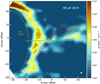 |
Fig. 2 ALMA Band 3 intensity integrated map of HC3N 10–9. The 3σ level is indicated on the colorbar with a horizontal white line, with σ = 0.01 Jy beam−1 km s−1. The positions of IRAS 16293 A and B are marked with a white star and filled circle, respectively. The dashed orange lines highlight the structures identified in this work. The arrows indicate the E–W (green) and NW–SE (red) outflow directions from source A. The white ellipse in the bottom-right corner indicates the synthesized beam. |
4 Analysis
4.1 Kinematics
In order to understand the nature of the N–S and west ridges, the gas velocity distributions were examined. The northern part of the N–S ridge is present only in the velocity range between 1.3 and 4.3 km s−1, while the west ridge is detected in the velocity range of 4–8 km s−1. We note that the systemic velocity of source A is 3.1 km s−1. The southern part of the N–S ridge presents components in both velocity ranges, and its distribution coincides with that of the southeastern part of the NW–SE outflow. It is thus possible that the southern part of the N–S ridge is in fact part of an outflow cavity rather than an envelope structure. Details and intensity integrated maps of both velocity ranges are given in Appendix B.
The low spectral resolution of HNC and HC3N, as well as the clumpy nature of HC5N, hinders a detailed kinematic analysis of the N–S ridge. However, some insight can still be obtained. A position velocity (PV) diagram was extracted from the HC5N 35–34 data cube (channel width = 0.049 km s−1) with a position angle of 34° and a width of 7 pixels (1.12′′), covering the extent of 33′′ from the map edge to the east of source A (Fig. 4). The resulting PV diagram, although clumpy, suggests a velocity increase as the distance to source A decreases (Fig. 4). The increase in velocity inversely proportional to distance is characteristic of free-falling (v ~ r−1∕2) or infalling (v ~ r−1) motion. Such curves are plotted over the HC5N PV diagramin Fig. 4 to show the trend; however, no estimate of the enclosed mass at any radius is made based on these curves.
Although our observations of HC3N 10–9 and HNC 1–0 were obtained with a low spectral resolution of only 0.8 km s−1, an indication of the velocity pattern can still be obtained by examining their centroid velocities along the N–S ridge. Both molecules show velocity inversely proportional to distance from source A; however, the velocities do not match with HC5N. The velocity discrepancy is due to several factors. From 33′′ to 10′′ from source A, HNC and HC3N show inverse P Cygni spectral profiles (Fig. 4, Positions 1 and 2). Although the locations are quite offset from source A, the continuum against which the line emission is absorbing is that of IRAS 16293. As shown in Bjerkeli et al. (2012), inverse P Cygni profiles can be detected out to 100′′ from the continuum source. The absorption becomes weaker with increased distance from the source, as is the case in the data presented here. This inverse P Cygni profile is an indication of infalling material but does not allow for centroid velocity analysis. At offsets below 10′′, the spectral profiles of HNC and HC3N become broad, while HC5N shows several peaks (Fig. 4, Position 3). This is consistent with the complex outflow and envelope morphology, and thus a centroid velocity cannot be reliably determined. Finally, about 5′′ from source A, the spectral profile of HNC shifts to the P Cygni profile (Fig. 4, Position 4), indicative of outflowing material, while HC3N presents a much broader spectral profile than HC5N. Hence, the kinematic analysis of HC3N and HNC is not inconsistent with that of HC5N but does not provide additional constraints.
The shift in velocity and spectral line profile along the northern part of the N–S ridge, together with the inverse P Cygni profile and velocity inversely proportional to distance from source A, indicates that this is an infalling structure within the IRAS 16293 cloud core. Further higher spectral resolution observations of HC3N and HNC with a larger field of view are necessary to provide a more detailed kinematic analysis; this would, in particular, allow the structure around source A to be disentangled and allow us to determine at what radius material is being delivered. Higher spatial resolution is needed to further characterize the infall motion and to determine whether source A1, A2, or both are accreting the bulk of the material.
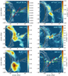 |
Fig. 3 ALMA Band 3 intensity integrated maps of the molecular species that show extended emission around IRAS 16293−2422. The 3σ level is indicated on the colorbar with a horizontal white or gray line. HC3N 10–9 is overlaid in contours with steps of 3, 5, 7, 9, and 15σ, with σ = 10 mJy beam−1 km s−1. The positions of IRAS 16293 A and B are marked with a star and circle, respectively. The dashed orange lines indicate the structures identified in this work. The arrows indicate the E–W (green) and NW-SE (red) outflow directions from source A. The white ellipses in the bottom-right corner indicate the beam of the observations. |
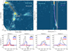 |
Fig. 4 Kinematic analysis of the N–S ridge. Top-left panel: integrated intensity map of HC5N (color scale) overlaid with HC3N contours, as in Fig. 3. The white star and circle mark sources A and B, respectively. The white ellipse in the bottom-right corner shows the beam size. Top-right panel: Cut used to make the PV diagram with source A located at offset 0 (indicated by the orange rectangle in the top-left panel). The vertical dotted lines mark the systemic velocity of A and B. The white and magenta lines show free-fall and infall curves, respectively. The velocity range with E–W-outflow-related emission is shown as the shaded area (4.5 and 5.1 km s−1) (Fig. B.1). Bottom row: HNC, HC3N, and HC5N spectra extracted from the corresponding positions marked in the top-left panel. The changes in peak velocity and line shape are signatures of moving gas. HNC and HC3N show an inverse P Cygni profile along the middle of the N–S ridge (Position 2, ~20′′ from source A), indicating infall. Near source A (Position 4, ~5′′) HNC shifts to a P Cygni profile, consistent with the presence of outflow in this region. |
4.2 Comparison with higher transitions
Data from PILS include HNC 4–3, HCN 4–3, and three transitions of HC3N: 37–36, 38–37, and 39–38 (Table 1). No line emission is detected from the transitions of HC5N within the frequency range of the PILS program (329.147–362.896 GHz). The PILS data, which combined 12 m array and ACA observations, recover scales from 0.5″ up to 13″ with a field of view of 16″. Thus, only the inner 16″ of the Band 3 observations can be compared. Figure 5 presents overlaid Band 7 (color) and Band 3 (contours) intensity integrated maps.
The three Band 7 transitions of HC3N all show an emission peak on source A, but no further extended structures are detected. The brightest transition, HC3N 38–37, is included in Fig. 5 for comparison. Similarly, HNC 4–3 peaks about 1′′ east of source A but presents no other significant extended emission.
In the direction of the southeastern outflow lobe, H13CO+ presents emission in both 1–0 and 4–3 transitions (Fig. 5) in a velocity range between 4 and 7 km s−1 (Fig. B.1). The velocity range and spatial agreement of both transitions suggests the southeastern H13CO+ arises from the outflow cavity walls. North of source A, H13CO+ 4–3 traces the material between sources A and B, along the dust bridge but not along the region where the N–S ridge is detected, similar to the 1–0 transition. Despite the different spatial distributions, both transitions are present between 1 and 4 km s−1 (Fig. B.1), indicating their envelope nature. The inner circular region around source A where H13CO+ is not present (Fig. 5) coincides with the 100 K radius (Jacobsen et al. 2018), tracing the water snow line (e.g., van ’t Hoff et al. 2018; Leemker et al. 2021). It is worth highlighting that the east-west outflow does not present H13CO+ emission in either transition. HCN 4–3 traces material that extends between sources A and B. While the HCN 1–0 emission traces both outflows driven by source A, the 4–3 transition mainly arises from the northwest–southeast outflow and part of the western outflow lobe cavity wall (van der Wiel et al. 2019).
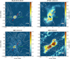 |
Fig. 5 ALMA Band 7 data (PILS; color scale) overlaid with Band 3 combined data (contours) for HC3N, H13CO+, HNC, and HCN. The 3σ level is indicated on the colorbar with a horizontal white or gray line. Panels are the size of the PILS Band 7 field of view. Contours are in steps of 3, 5, 7, 10, 15, 20, 30, 40, 50, and 80σ, where σ = 70 mJy beam−1 km s−1 for HCN; 3, 5, 10, 15, 20, 25, 30, 40, and 50σ, where σ = 7 mJy beam−1 km s−1 for HNC; 3, 5, 6, 7, 8, 15, 30, and 50σ, where σ = 10 mJy beam−1 km s−1 for HC3N; and 2, 3, and4σ, where σ = 50 mJy beam−1 km s−1 for H13CO+. The positions of IRAS 16293 A and B are marked with a star and circle, respectively. The arrows indicate the E–W (green) and NW-SE (red) outflow directions from source A. The white circle and gray ellipse show the Band 7 (PILS) and Band 3 beams, respectively. |
4.3 Line ratios
Spherical envelope models of IRAS 16293 indicate gas and dust temperatures of ~40, 30, and 20 K at radii of 500, 1000, and 2000 AU, respectively (Schöier et al. 2002; Crimier et al. 2010). Three-dimensional modeling of the dust emission (including the spectral energy distribution) in the IRAS 16293 envelope (Jacobsen et al. 2018) shows dust temperatures of 30 K out to a radius of 750 AU to the east, south, and west of source A; dust temperatures drop below 30 K beyond 500 AU north of source A in the same model. Gas temperatures derived from molecular line emission observations within 1000 AU of source A (Murillo et al. 2018b) range from 20 K (DCO+ at the disk edge) to 150 K (outflow cavity traced in c-C3H2). The physical conditions of the low-J molecular line emission presented in this work are determined in two ways: 1) via the HCN/HNC abundance ratio and 2) via the line ratio of the same molecule in two transitions.
Recently, Hacar et al. (2020) demonstrated empirically that the HCN 1–0/HNC 1–0 ratio is a probe of gas temperature in the range of 14 to 40 K. The HCN/HNC line intensity ratio is related to the gas kinetic temperature with the following relations, derived by Hacar et al. (2020):
 (1)
(1)
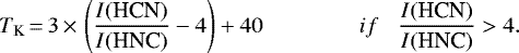 (2)
(2)
Both HCN and HNC are formed in a 1:1 ratio from HCNH+ dissociative recombination. The destruction of HNC in reactions with H and O is more efficient with temperature. At higher temperatures, HNC is isomerized, thus increasing the abundance of HCN.
To produce a ratio map of HCN and HNC for IRAS 16293, the images need to have the same range of recovered scales. An HNC map from our combined Band 3 data was generated using the same (u, v) range as the HCN data. The resulting HNC map was then convolved with the same beam as the HCN map, 1.34′′ × 0.94′′. Intensity integrated maps of HCN and HNC were then generated, clipped at the 3σ level for HNC and the 1σ level for HCN. The maps were then converted to units of K km s−1 (Fig. 6). The mean flux density in mJy beam−1 km s−1 was converted to brightness temperature in K km s−1 by Tmb = 1.36 λ2∕θ2 Iν, where λ is the wavelength of the molecular transition in centimeters, θ is the synthesized beam in arcseconds, and Iν is the flux density in mJy beam−1 km s−1. The HCN/HNC ratio map is shown in Fig. 6, where the color scale is limited by the HNC 3σ level and the HCN 3σ level is indicated by black contours. Temperatures derived from ratios outside of the black contours are upper limits. The lack of HCN emission indicates that the N–S ridge is mainly composed of cold gas (T ~ 20 K). This is consistent with the chemistry of HCN and HNC and is reflected by the upper limits of the HCN/HNC ratio.
Along the N–S ridge, the HCN/HNC ratio indicates a mean gas temperature of ~25 K when only points with HCN above 3 are considered, and ~20 K when all points along the N–S ridge shown in Fig. 6 are considered. For regions where both isomers are present, the typical mean error is 9 K. There are a few pixels with HCN/HNC ratios between 4 and 8.5, along the edges of the N–S ridge and HCN blobs, which would suggest pockets of gas with temperatures ≥40 K. Not considering these pixels with higher ratios, the gas temperature ranges between 10 K and 30 K along the N–S ridge. One caveat that should be considered is that the HCN blobs are evenly separated and aligned from northeast to southwest, which indicates that they are likely artifacts of the uv coverage rather than real structure. This suggests that the N–S ridge is mainly composed of cold gas, with perhaps a few clumps of warmer gas. The HCN/HNC ratio along the west ridge gives an upper limit mean of ~30 K (Fig. 6). The origin of the warm pockets along the N–S ridge is not clear, given the lack of a heating source or dust and the low envelope dust and gas temperatures derived from models (but see Sect. 5.3).
In the region around sources A and B, where HCN emission is predominant, the HCN/HNC ratio ranges between 1.5 and 82, implying temperatures from 15 K to well above 40 K. However, kinetic temperatures above 40 K are not well constrained by the empirical method of Hacar et al. (2020). This temperature structure is consistent with the envelope dust and gas temperature derived from models (e.g., Crimier et al. 2010; Jacobsen et al. 2018) and with the fact that the bulk of protostellar heating escapes through the outflow cavities.
Constraints on the density of the N–S ridge, as well as the inner region around sources A and B, can be obtained by comparing the low-J (Band 3) and higher-J (Band 7) transitions of HNC, HC3N, and HCN together with the gas kinetic temperatures derived from the HCN/HNC ratio. Details of the analysis are presented in Appendix C and Fig. C.1. The comparison indicates that the N–S ridge has H2 densities of ~105 cm−3, while the inner region has H2 densities that are one to two orders of magnitude higher for temperatures between 10 and 40 K. These physical parameters are consistent with envelope models of IRAS 16293.
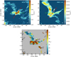 |
Fig. 6 Intensity integrated map of HCN (top left) and HNC (top right) in K km s−1. The HCN map was masked at 1σ (0.07 Jy beam km s−1) and the HNC map at 3σ (0.02 Jy beam km s−1) before being converted to brightness temperature. The 3σ level is indicated on the colorbar with a horizontal black or white line. Source A and B positions are marked with a star and circle, respectively. The arrows indicate the E–W (green) and NW–SE (red) outflow directions from source A. The white ellipse in the bottom-left corner indicates the map beam size. The gas kinetic temperature (TK) map, obtained from HCN/HNC and Eqs. (1) and (2), is shown in the bottom panel. The color scale is limited by the HNC 3σ level. The black contours indicate the HCN 3σ level, outside of which TK is an upperlimit. The lack of HCN emission indicates that the N–S ridge is mainly composed of cold gas, which is constrained by the ratio upper limits. Temperatures above 40 K are not well constrained by the HCN/HNC ratio, and hence the temperature scale only runs up to 49 K. |
5 Discussion
The observations presented in this work reveal two extended structures present in the cloud core of IRAS 16293, both related to source A and traced in several molecular species. The physical and chemical conditions of the two structures, the N–S and west ridges, are summarized in this section and placed in the context of previous work. The main observational result of this work is the uneven distribution of material within the cloud core of a multiple protostellar system.
5.1 Accretion stream
The N–S ridge is composed of cold gas (~15 K), with a few clumps at ≤40 K, and presents a layered molecular gas structure but no dust continuum. The N–S ridge is best traced in HNC, HC3N, and HC5N. Partial N2H+ and faint H13CO+ along the N–S ridge, together with CO only tracing the outflows driven by source A (van der Wiel et al. 2019), indicate that these molecules are not good tracers of accretion flows for IRAS 16293. The N–S ridge is only present at envelope velocities (0.8–4.3 km s−1). Kinematic analysis of HC5N, HC3N, and HNC suggests infalling gas along the northern part of the N–S ridge, in particular the presence of HNC and HC3N inverse P Cygni profiles. Based on these results, we propose that the northern part of the N–S ridge is a cold accretion structure that is transferring material from the outer parts of the cloud core onto IRAS 16293 A. The nature of the southern part of the N–S ridge cannot be fully determined with the current data due to spatial overlap with the southeastern lobe of the NW-SE outflow. We need higher spectral resolution observations of HC3N and HNC toconfirm the kinematic structure of the N–S ridge. Interestingly, no connection between the N–S ridge and source B is detected.
Accretion flows, or accretion streamers, have previously been detected in other embedded sources at 103 –104 AU scales (Alves et al. 2019, 2020; Pineda et al. 2020). In addition, models of multiple protostellar formation also show such long and narrow structures readily forming in the cloud core of these systems (e.g., Offner et al. 2010; Kuffmeier et al. 2019). Thus, the scenario of the N–S ridge being an accretion streamer feeding material onto IRAS 16293 A is likely. However, the N–S ridge is only transferring material to one of the components in the wide multiple protostellar system. Continuous delivery of envelope gas onto the circumstellar environment of source A, but not source B, could explain the difference in multiplicity and bolometric luminosity (18 L⊙ vs. 3 L⊙, Jacobsen et al. 2018) between the two sources. This is supported by a rough estimate of accretion rates, the derivation of which is detailed in Appendix D. The northern part of the N–S ridge has an estimated accretion rate of 7 × 10⁻⁷ to a few 10−6 M⊙ yr−1. Conversely, assuming that accretion luminosity is equal to the bolometric luminosity of source A, Lacc = Lbol = 18 L⊙, the accretion rate is about 8 × 10⁻⁷ M⊙ yr−1. With the same luminosity assumption, source B (Lbol = 3 L⊙) would have an accretion rate of a few 10−7 M⊙ yr−1. Preferential accretion of material could be key in multiple protostellar system formation and evolution (Murillo et al. 2018a). In particular, uneven delivery of material in wide multiple protostars (separations larger than the disk radius) could provide insight into systems with components at different evolutionary stages (Murillo et al. 2016).
It should be stressed that the N–S ridge is cleanly traced in HC3N, suggesting it could be a good tracer for cold gas accretion flows in the cloud core of embedded protostars. Indeed, HC3N traces the accretion flow in Per-emb 2 (IRAS 03292+3039; Pineda et al. 2020). However, the N–S ridge is also well traced in HNC and HC5N and partially in N2H+, with faint H13CO+ and HCN emission. Tracing accretion flows in cloud cores using several of the same molecules used to trace filamentary structures on molecular cloud scales (R > 104 AU; Arzoumanian et al. 2013; Hacar et al. 2013; Fernández-López et al. 2014; Hacar et al. 2017, 2020) makes it possible to eventually trace the transfer of material from parsec scales down to protostellar scales. In addition, HNC is commonly detected in embedded protostellar sources (~7000 AU; Murillo et al. 2018a) and is thus also a potential good tracer for cold gas accretion flows in cloud cores. This is important since not all embedded protostars may have carbon chains present in the cloud core (e.g., Murillo et al. 2018a), in particular cyanopolyynes, which would lead to non-detections of accretion flows if only this tracer were used. In general, the physical conditions of a cloud core should be considered when determining which molecular species to use for tracing accretion flows.
5.2 Outflow cavity walls
The west ridge, detected in HC3N, HC5N, and HNC, is related to the E–W outflow and is composed of cold gas. The spatial and velocity distributions of the west ridge are consistent with the redshifted western outflow cone detected in 12CO 3–2 (8–14 km s−1) and with the northern cavity wall of the same lobe detected in other molecules (4–7 km s−1; van der Wiel et al. 2019).
The molecules N2H+ and H13CO+ show emission along the southeastern lobe of the NW-SE outflow. The chemistry of these species provides gas temperature constraints. Given that N2H+ is present when CO is frozen out (gas and dust temperature below 20–30 K), the emission traces the outer cavity wall rather than the outflow itself. On the other hand, H13CO+ requires CO in the gas phase (temperatures above 20–30 K) to form, and it reacts with water vapor (gas temperature above 100 K). Thus, H13CO+ traces a warmer part of the outflow cavity with a temperature range between 30 and 100 K, which is consistent with the gas temperature range inferred from c-C3H2, 120–155 K (Murillo et al. 2018b).
A comparison of the observed molecular species and derived conditions indicates that the NW–SE outflow is significantly warmer than the E–W outflow. This is consistent with the E–W outflow being more prominent in the Band 3 observations than in the Band 7 observations. The contrast of molecular species tracing each outflow, and each respective cavity wall, demonstrates the layered nature of these objects and the impact of the driving source on the chemical structure of the cavity. This could provide a further constraint in determining which source in the close binary A1+A2 drives each outflow.
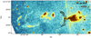 |
Fig. 7 Spitzer IRAC2 image of IRAS 16293−2422 (color scale), overlaid with HC3N (contours). The IRAC2 image shows the E–W outflow cavities but does not show structures relating to the NW-SE outflow. The HC3N west ridge matches with the western lobe of the E–W outflow. The N–S ridge is not related to the outflow cavity walls, but its chemistry may be impacted by the eastern lobe of the E–W outflow. |
5.3 Large-scale scenario
The layered molecular gas structure of the N–S ridge and the presence of HC3N and HC5N at these scales suggest that the N–S ridge gas is externally heated. A possible source of heating is the UV-emitting jet shocks within the eastern cavity of the E–W outflow seen in large-scale Spitzer IRAC2 images (Fig. 7). Heating of the N–S ridge from one side also explains the layered nature of the gas, with N2H+ located farthest from the outflow cavity, consequently implying a temperature gradient from east to west. It could be argued that the N–S ridge is a limb brightening around the outflow cavity. However, the physical conditions and chemistry along the N–S ridge suggest otherwise. The velocity range of the N–S ridge already indicates that it is not part of the outflow cavity, but rather the envelope. In addition, the different chemical structures of the N–S ridge and the west ridge, which is part of the E–W outflow cavity wall, also provide evidence against the limb brightening scenario of the N–S ridge. The limited kinematic analysis possible with the present data hints at the infalling nature of the N–S ridge, but higher spectral resolution is needed to probe the kinematics of the ridge.
Something worth noting is the lack of carbon chain molecules (Cn Hn−1), while cyanopolyynes (HCnN where n = 3, 5, 7...) are readily present. A transition of c-C3H2 at 93.16 GHz (log10 Aij = –4.76, Eup = 92 K) falls in the frequency range of our Band 3 observations, but it is not detected. The possible reasons for the lack of extended cyclopropenylidene emission are briefly explored below.
The critical density of c-C3H2 at 93.16 GHz lies between 103 and 104 cm−3 for a temperature range of 10 to 100 K, while that of HC3N 10–9 is about 104 cm−3 for a similar temperature range. Hence, the lack of c-C3H2 is not due to density or gas temperature. In Band 7 observations, c-C3H2 is detected mainly within the NW-SE outflow cavity with gas temperatures above 100 K and is spatially anticorrelated with C2H (Murillo et al. 2018b). Hence, the lack of detected c-C3H2 may be due to chemistry rather than physical conditions. It is interesting to note that HC3N is readily formed through the following gas phase reactions (Loison et al. 2014, 2017):


with the former and latter reactions also being valid for HCN and l-C3H2, respectively.The latter reaction, while minor, is non-negligible (Loison et al. 2017), and the abundance of nitrogen in the gas phase as evidenced by N2H+ makes it even more viable. Further interaction between C2H and HC3N can lead to the formation of HC5N. Similarly, the Band 3 observations presented here show that HNC is also present. Hence, the lack of carbon chains and the presence of cyanopolyynes are likely due to the above reactions. This then explains the layered structure observed along the N–S ridge, in particular the offset between HNC and the cyanopolyynes. Furthermore, it would also provide a reason why HC3N and HC5N are present in the E–W outflow but are much weaker in the NW-SE outflow, which does present c-C3H2 emission in Band 7 observations. The presence of HNC and HCN in the southeastern outflow cavity would suggest that the non-detection of C2H (Murillo et al. 2018b) is due to the reaction between these molecules producing HC3N.
The results presented in this work demonstrate the importance of observing a broad range of frequencies and molecular lines toward protostellar systems, as well as the capacity of ALMA to probe cloud core structure, in particular with short baselines. To identify accretion flows or streams, and differentiate them from outflow structures, the cloud core needs to be characterized at a range of scales with molecular species tracing cold and warm gas. Sufficient spectral resolution is also crucial for examining the velocity structure.
6 Conclusions
We present ALMA Band 3 (3 mm) observations of IRAS 16293−2422. The data presented in this work include observations of the low-J transitions of the cyanopolyynes HC3N and HC5N, along with HNC, HCN, H13CO+, N2H+, and SiO. Further comparison with higher-J transitions was done using ALMA Band 7 data from the PILS program (Jørgensen et al. 2016).
The results of this work can be summarized in the following points:
- 1.
Extended, cold gas (≤20 K) structures on scales of a few hundred AU up to 6000 AU (40′′) are detected with our Band 3 observations toward IRAS 16293 with a spatial resolution of 130 AU. Two main structures are identified: a N–S ridge and a west ridge. These are traced best in HC3N, HNC, and HC5N. The molecules H13CO+ and N2H+ only partially trace the N–S ridge. No carbon chain molecules are detected. These structures do not present a counterpart in dust continuum or in higher transitions (Band 7) of the same molecular species;
- 2.
Our results delve into the detailed structure of sources A and B providing, an updated scenario of this system. We propose the following scenario based on the results of the current data. Envelope material from a few thousand AU is being delivered, and accreted, by IRAS 16293 A, while IRAS 16293 B can accrete only its immediate circumstellar material. This scenario could explain the different bolometric luminosities of sources A and B (18 and 3 L⊙, respectively) and the binarity of IRAS 16293 A;
- 3.
The molecules tracing the N–S ridge are slightly spatially offset relative to one another, generating a layered structure. The layering and lack of carbon chains along the N–S ridge can be explained by chemical processes, namely the reaction of carbon chains with HNC and nitrogen to produce HC3N and HC5N. Furthermore, the chemical structure of the N–S ridge helps in determining its nature;
- 4.
The west ridge traces part of the northern cavity wall of the western outflow lobe. The difference in molecular species present in each of the outflows driven by IRAS 16293 A, and their cavity walls, suggests different excitation conditions produced by the driving sources.
The results presented here show the importance of streamers in shaping individual protostellar components, and their circumstellar environment, in multiple protostellar systems. This work also demonstrates the importance of multifrequency observationsand a range of spatial resolutions for a complete picture of the physical structure of protostellar systems, multiple or single. Future observations of the extended protostellar cloud core environment that compare low- and high-J lines will prove invaluable to further understanding how material is structured and distributed among components in multiple protostellar systems. Combining this information from cloud core to disk scales will enable a better understanding of the formation and evolution of multiple protostellar systems.
Acknowledgements
This paper made use of the following ALMA data: ADS/JAO.ALMA 2013.1.00278.S, 2015.1.01193.S, and 2017.1.00518.S. ALMA is a partnership of ESO (representing its member states), NSF (USA), and NINS (Japan), together with NRC (Canada) and NSC and ASIAA (Taiwan), in cooperation with the Republic of Chile. The Joint ALMA Observatory is operated by ESO, AUI/NRAO, and NAOJ. N.M.M. acknowledges support from RIKEN Special Postdoctoral Researcher Program. This project has received funding from the European Research Council (ERC) under the European Union’s Horizon 2020 research and innovation programme (grant agreement no. 851435 to A.H., and No. 646908 to J.K.J.). The research of J.K.J. is furthermore supported by the Independent Research Fund Denmark (grant number 0135-00123B). D.H. acknowledges support from the EACOA Fellowship from the East Asian Core Observatories Association. D.H. is supported by CICA through a grant and grant number 110J0353I9 from the Ministry of Education of Taiwan.
Appendix A Spectra
ALMA Band 3 spectra were extracted from the three locations shown in Fig. 1: on source A; ~1′′ west of source B; and an off- source position 12′′ east of source B and away from the outflow directions. Spectra were extracted using a single pixel of the im- age, with the pixel size being 0.16′′. The resulting spectra are presented in Fig. A.1. The extracted spectra show both source A and B to be line rich, with line densities of ~120 lines/GHz at 86, 87, and91 GHz, and 34 lines/GHz at 93 GHz. In contrast, the off-source position has a line density of 8 lines/GHz.
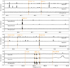 |
Fig. A.1 ALMA Band 3 spectra extracted from three positions: source A; source B (~1′′ off), where the peak of emission is located; and an off-source position 12′′ to the east of source B. Positions are shown in the right panel of Fig. 1. For the purpose of comparison, the off-source spectrum is multiplied by a factor of 3, while the HCN spectra for source A and B are multiplied by 0.3. The molecular species that show up in the off-source position are labeled. In addition, c-C3H2 is also labeled for reference. We note the chemical richness of the source positions in contrast to the off-source position. |
Appendix B Kinematics: Envelope versus outflow
The N-S and west ridges present different velocity ranges (Fig. B.1). The N-S ridge is present only at velocities between 1.3 and 4.3 km s−1. Given the systemic velocities of sources A and B, 3.1 and 2.7 km s−1, respectively,the N-S ridge mainly traces envelope material, particularly in the northern part of the N-S ridge. In contrast, the west ridge is characterized by emission at the velocity range of 4–8 km s−1, which is consistent with the observed velocity range for the red part of the outflows (van der Wiel et al. 2019). Detailed kinematic analysis of both ridges cannot be performed with HC3N, HNC, or H13CO+ due to the low spectral resolution of the data, 0.8 km s−1. While N2H+ has a higher spectral resolution of 0.049 km s−1, strong absorption due to filtering prevents us from extracting the detailed kinematic in- formation from the cold gas traced by N2H+.
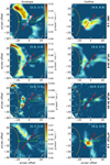 |
Fig. B.1 Intensity integrated maps aiming to disentangle the envelope and outflow contributions to the observed emission. The velocity range over which each map was integrated is given in square brackets in units of km s−1. The positions of IRAS 16293 A and B are marked with a star and circle, respectively. The arrows indicate the E-W (green) andNW-SE (red) outflow directions from source A. The white ellipse in the bottom-right corner shows the beam. |
Appendix C Ratios of high-J versus low-J transitions
The non-detection of Band 7 high-J transitions of HNC and HCN along the N-S ridge provides upper limits on the physical conditions of this structure. While the line ratio of HC3N would provide further constraints, the available molecular data file only covers up to J=37 (Faure et al. 2016). Of the Band 7 HC3N transitions, the 38–37 shows the most extended emission, while the 37–36 transition is concentrated on source A. Compar- ison of the low- and high-J transitions is made within the Band 7 field of view around source A and where the N-S ridge is located (Fig. 5). If the noise level of the Band 7 observations is taken as the upper limit for the high-J HCN, HNC, and HC3N transitions, the peak intensity in Band 7 is at least an order of magnitude lower than in Band 3.
Line ratio models were done using non-LTE slab calculations with RADEX (van der Tak et al. 2007) with molecular data files (Dumouchel et al. 2010; Faure et al. 2007) obtained from the Leiden Atomic and Molecular Database (Schöier et al. 2005; van der Tak et al. 2020). A line width of 2 km s−1 and a column density of 1013 cm−1 were adopted. The H2 density is constrained by the envelope models of IRAS 16293 (Crimier et al. 2010), which indicate H2 densities below 106 cm−3 at radii of 30 to 40′′, the equivalent to the edge of our Band 3 maps. At radii below 10′′, the H2 densities are between 106 and 107 cm−3, increasing to ~109 cm−3 at the continuum peak of IRAS 16293 A. Figure C.1 shows the modeled ratios, with the temperature and density constraints obtained from the HCN/HNC map and envelope models, respectively.
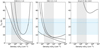 |
Fig. C.1 Calculated brightness temperature ratios for HCN 4–3/1–0 (left), HNC 4–3/1–0 (center), and HC3N 37–36/10–9 (right). Contours show modeled ratios assuming a column density of 1013 cm−2 and a line width of 2 km s−1 for all three molecular species. The light blue shaded region shows the temperature range derived from the HCN/HNC ratio, with the blue line indicating the mean gas temperature. The gray shaded area shows the density range for the N-S ridge derived from envelope models. |
Along the N-S ridge, HCN 4–3/1–0 ~ 0.02 and HNC 4–3/1–0 ~ 0.001. These are consistent with the temperature and density constraints obtained from the HCN/HNC ratio and the envelope model. Around the IRAS 16293 sources, the HCN ratio is be- tween 0.1 and 0.2. Considering the H2 densities from envelope models around these sources, above 108 cm−3, the temperatures go well above 40 K, consistent with the HCN/HNC.
Appendix D Accretion rate estimates
Assuming the northern part of the N-S ridge is infalling, and thus delivering material onto source A, a rough estimate of the accretion rates can be done. For the mass of the N-S ridge, a cylindrical volume can be assumed using a radius of 2.5′′ and a length of 40′′. Based on the line ratio analysis, an H2 density of 106 cm−3 is assumed. This results in a mass of 0.014 M⊙. The free-fall timescale was obtained by the equation tff = (R3 / GM)1∕2, where R and M are the enclosed radius and mass, re- spectively, and G is the gravitational constant. Using R = 20′′ or 10′′ and an enclosed mass of 2 M⊙ (Maureira et al. 2020), we get an accretion rate between 7×10⁻⁷ and 10−6 M⊙ yr−1. Changing the H2 density (0.5 to 5 × 106 cm−3) or the enclosed mass (e.g., to 4 M⊙) only changes the accretion rate by a few M⊙ yr−1, but it stayswithin the 10−7 to 10−6 M⊙ yr−1 range.
The accretion rate derived above needs to be compared to an accretion rate on source A. The best estimate for this is from ac- cretion luminosity, Lacc. The accretion rate, Ṁacc, is thus given by the relation Ṁacc = Lacc / RGM*, where G is the gravitational constant, M* is the mass of the central source, and R is the protostellar radius, assumed to be 3 R⊙ (Dunham et al. 2010; Hsieh et al. 2019). Assuming that Lbol = Lacc = 18 L⊙ for source A and a combined central source mass of 2 M⊙ (Maureira et al. 2020), the accretion rate is about 8×10⁻⁷ M⊙ yr−1. This accretion rate increases if only one of the components in the close binary is re- ceiving material. Making similar assumptions for source B (Lbol = Lacc = 3 L⊙) yields an accretion rate of a few 10−7 M⊙ yr−1.
Comparing the accretion rate from luminosity for source A to that derived for the N-S ridge further supports the scenario that the northern part of the N-S ridge is likely an accretion flow that delivers material. Further high spectral resolution observations with a larger field of view are necessary to confirm this scenario.
References
- Akiyama, E., Vorobyov, E. I., Baobabu Liu, H., et al. 2019, AJ, 157, 165 [Google Scholar]
- Alves, F. O., Caselli, P., Girart, J. M., et al. 2019, Science, 366, 90 [NASA ADS] [CrossRef] [Google Scholar]
- Alves, F. O., Cleeves, L. I., Girart, J. M., et al. 2020, ApJ, 904, L6 [NASA ADS] [CrossRef] [Google Scholar]
- Arzoumanian, D., André, P., Peretto, N., & Könyves, V. 2013, A&A, 553, A119 [NASA ADS] [CrossRef] [EDP Sciences] [Google Scholar]
- Arzoumanian, D., Furuya, R. S., Hasegawa, T., et al. 2021, A&A, 647, A78 [NASA ADS] [CrossRef] [EDP Sciences] [Google Scholar]
- Bate, M. R., & Bonnell, I. A. 1997, MNRAS, 285, 33 [NASA ADS] [CrossRef] [Google Scholar]
- Belloche, A., Maury, A. J., Maret, S., et al. 2020, A&A, 635, A198 [NASA ADS] [CrossRef] [EDP Sciences] [Google Scholar]
- Bergin, E. A.,& Tafalla, M. 2007, ARA&A, 45, 339 [NASA ADS] [CrossRef] [Google Scholar]
- Bergman, P., Parise, B., Liseau, R., & Larsson, B. 2011, A&A, 527, A39 [NASA ADS] [CrossRef] [EDP Sciences] [Google Scholar]
- Bjerkeli, P., Liseau, R., Larsson, B., et al. 2012, A&A, 546, A29 [NASA ADS] [CrossRef] [EDP Sciences] [Google Scholar]
- Bondi, H. 1952, MNRAS, 112, 195 [Google Scholar]
- Bonnor, W. B. 1956, MNRAS, 116, 351 [NASA ADS] [CrossRef] [Google Scholar]
- Cazzoli, G., Cludi, L., Buffa, G., & Puzzarini, C. 2012, ApJS, 203, 11 [NASA ADS] [CrossRef] [Google Scholar]
- Ceccarelli, C., Castets, A., Caux, E., et al. 2000, A&A, 355, 1129 [NASA ADS] [Google Scholar]
- Creswell, R. A., Pearson, E. F., Winnewisser, M., & Winnewisser, G. 1976, Zeitsch. Naturf. A, 31, 221 [NASA ADS] [CrossRef] [Google Scholar]
- Crimier, N., Ceccarelli, C., Maret, S., et al. 2010, A&A, 519, A65 [NASA ADS] [CrossRef] [EDP Sciences] [Google Scholar]
- Delucia, F., & Gordy, W. 1969, Phys. Rev., 187, 58 [NASA ADS] [CrossRef] [Google Scholar]
- de Lucia, F. C., & Helminger, P. A. 1977, J. Chem. Phys., 67, 4262 [Google Scholar]
- Dumouchel, F., Faure, A., & Lique, F. 2010, MNRAS, 406, 2488 [NASA ADS] [CrossRef] [Google Scholar]
- Dunham, M. M., Evans, N. J., Bourke, T. L., et al. 2010, ApJ, 721, 995 [NASA ADS] [CrossRef] [Google Scholar]
- Ebert, R. 1955, in Liege International Astrophysical Colloquia, 6, Liege International Astrophysical Colloquia, 666 [Google Scholar]
- Endres, C. P., Schlemmer, S., Schilke, P., Stutzki, J., & Müller, H. S. P. 2016, J. Mol. Spectrosc., 327, 95 [NASA ADS] [CrossRef] [Google Scholar]
- Faure, A., Varambhia, H. N., Stoecklin, T., & Tennyson, J. 2007, MNRAS, 382, 840 [Google Scholar]
- Faure, A., Lique, F., & Wiesenfeld, L. 2016, MNRAS, 460, 2103 [NASA ADS] [CrossRef] [Google Scholar]
- Fernández-López, M., Arce, H. G., Looney, L., et al. 2014, ApJ, 790, L19 [Google Scholar]
- Ginski, C., Facchini, S., Huang, J., et al. 2021, ApJ, 908, L25 [NASA ADS] [CrossRef] [Google Scholar]
- Hacar, A., Tafalla, M., Kauffmann, J., & Kovács, A. 2013, A&A, 554, A55 [NASA ADS] [CrossRef] [EDP Sciences] [Google Scholar]
- Hacar, A., Tafalla, M., & Alves, J. 2017, A&A, 606, A123 [NASA ADS] [CrossRef] [EDP Sciences] [Google Scholar]
- Hacar, A., Bosman, A. D., & van Dishoeck, E. F. 2020, A&A, 635, A4 [NASA ADS] [CrossRef] [EDP Sciences] [Google Scholar]
- Harsono, D., van Dishoeck, E. F., Bruderer, S., Li, Z. Y., & Jørgensen, J. K. 2015, A&A, 577, A22 [NASA ADS] [CrossRef] [EDP Sciences] [Google Scholar]
- Hayashi, C. 1966, ARA&A, 4, 171 [NASA ADS] [CrossRef] [Google Scholar]
- Hsieh, T.-H., Murillo, N. M., Belloche, A., et al. 2018, ApJ, 854, 15 [NASA ADS] [CrossRef] [Google Scholar]
- Hsieh, T.-H., Murillo, N. M., Belloche, A., et al. 2019, ApJ, 884, 149 [Google Scholar]
- Jaber Al-Edhari, A., Ceccarelli, C., Kahane, C., et al. 2017, A&A, 597, A40 [NASA ADS] [CrossRef] [EDP Sciences] [Google Scholar]
- Jacobsen, S. K., Jørgensen, J. K., van der Wiel, M. H. D., et al. 2018, A&A, 612, A72 [NASA ADS] [CrossRef] [EDP Sciences] [Google Scholar]
- Jørgensen, J. K., Schöier, F. L., & van Dishoeck, E. F. 2005, A&A, 435, 177 [NASA ADS] [CrossRef] [EDP Sciences] [Google Scholar]
- Jørgensen, J. K., Bourke, T. L., Nguyen Luong, Q., & Takakuwa, S. 2011, A&A, 534, A100 [NASA ADS] [CrossRef] [EDP Sciences] [Google Scholar]
- Jørgensen, J. K., van der Wiel, M. H. D., Coutens, A., et al. 2016, A&A, 595, A117 [Google Scholar]
- Kirk, H., Myers, P. C., Bourke, T. L., et al. 2013, ApJ, 766, 115 [Google Scholar]
- Kuffmeier, M., Calcutt, H., & Kristensen, L. E. 2019, A&A, 628, A112 [NASA ADS] [CrossRef] [EDP Sciences] [Google Scholar]
- Larson, R. B. 1969, MNRAS, 145, 271 [Google Scholar]
- Leemker, M., van’t Hoff, M. L. R., Trapman, L., et al. 2021, A&A, 646, A3 [EDP Sciences] [Google Scholar]
- Li, Z.-Y., Krasnopolsky, R., & Shang, H. 2013, ApJ, 774, 82 [NASA ADS] [CrossRef] [Google Scholar]
- Li, Z. Y., Banerjee, R., Pudritz, R. E., et al. 2014, in Protostars and Planets VI, eds. H. Beuther, R. S. Klessen, C. P. Dullemond, & T. Henning, 173 [Google Scholar]
- Loison, J.-C., Wakelam, V., & Hickson, K. 2014, MNRAS, 443, 398 [NASA ADS] [CrossRef] [Google Scholar]
- Loison, J.-C., Agúndez, M., Wakelam, V., et al. 2017, MNRAS, 470, 4075 [Google Scholar]
- Matsumoto, T., Onishi, T., Tokuda, K., & Inutsuka, S.-i. 2015, MNRAS, 449, L123 [NASA ADS] [CrossRef] [Google Scholar]
- Matsumoto, T., Saigo, K., & Takakuwa, S. 2019, ApJ, 871, 36 [CrossRef] [Google Scholar]
- Maureira, M. J., Pineda, J. E., Segura-Cox, D. M., et al. 2020, ApJ, 897, 59 [NASA ADS] [CrossRef] [Google Scholar]
- McMullin, J. P., Waters, B., Schiebel, D., Young, W., & Golap, K. 2007, in ASP Conf. Ser., 376, Astronomical Data Analysis Software and Systems XVI, eds. R. A. Shaw, F. Hill, & D. J. Bell, 127 [Google Scholar]
- Mizuno, A., Fukui, Y., Iwata, T., Nozawa, S., & Takano, T. 1990, ApJ, 356, 184 [NASA ADS] [CrossRef] [Google Scholar]
- Monsch, K., Pineda, J. E., Liu, H. B., et al. 2018, ApJ, 861, 77 [NASA ADS] [CrossRef] [Google Scholar]
- Murillo, N. M., van Dishoeck, E. F., Tobin, J. J., & Fedele, D. 2016, A&A, 592, A56 [NASA ADS] [CrossRef] [EDP Sciences] [Google Scholar]
- Murillo, N. M., van Dishoeck, E. F., Tobin, J. J., Mottram, J. C., & Karska, A. 2018a, A&A, 620, A30 [NASA ADS] [CrossRef] [EDP Sciences] [Google Scholar]
- Murillo, N. M., van Dishoeck, E. F., van der Wiel, M. H. D., et al. 2018b, A&A, 617, A120 [NASA ADS] [CrossRef] [EDP Sciences] [Google Scholar]
- Narayanan, G., Walker, C. K., & Buckley, H. D. 1998, ApJ, 496, 292 [NASA ADS] [CrossRef] [Google Scholar]
- Offner, S. S. R., Kratter, K. M., Matzner, C. D., Krumholz, M. R., & Klein, R. I. 2010, ApJ, 725, 1485 [Google Scholar]
- Ortiz-León, G. N., Loinard, L., Kounkel, M. A., et al. 2017, ApJ, 834, 141 [Google Scholar]
- Oya, Y., Sakai, N., López-Sepulcre, A., et al. 2016, ApJ, 824, 88 [Google Scholar]
- Oya, Y., Moriwaki, K., Onishi, S., et al. 2018, ApJ, 854, 96 [NASA ADS] [CrossRef] [Google Scholar]
- Palmeirim, P., André, P., Kirk, J., et al. 2013, A&A, 550, A38 [NASA ADS] [CrossRef] [EDP Sciences] [Google Scholar]
- Penston, M. V. 1969, MNRAS, 144, 425 [NASA ADS] [CrossRef] [Google Scholar]
- Peretto, N., Fuller, G. A., Duarte-Cabral, A., et al. 2013, A&A, 555, A112 [NASA ADS] [CrossRef] [EDP Sciences] [Google Scholar]
- Pickett, H. M., Poynter, R. L., Cohen, E. A., et al. 1998, J. Quant. Spec. Radiat. Transf., 60, 883 [Google Scholar]
- Pineda, J. E., Goodman, A. A., Arce, H. G., et al. 2011, ApJ, 739, L2 [NASA ADS] [CrossRef] [Google Scholar]
- Pineda, J. E., Maury, A. J., Fuller, G. A., et al. 2012, A&A, 544, L7 [NASA ADS] [CrossRef] [EDP Sciences] [Google Scholar]
- Pineda, J. E., Segura-Cox, D., Caselli, P., et al. 2020, Nat. Astron., 4, 1158 [NASA ADS] [CrossRef] [Google Scholar]
- Rivilla, V. M., Beltrán, M. T., Vasyunin, A., et al. 2019, MNRAS, 483, 806 [NASA ADS] [CrossRef] [Google Scholar]
- Sadavoy, S. I., Myers, P. C., Stephens, I. W., et al. 2018, ApJ, 869, 115 [NASA ADS] [CrossRef] [Google Scholar]
- Sánchez-Monge, Á., Schilke, P., Ginsburg, A., Cesaroni, R., & Schmiedeke, A. 2018, A&A, 609, A101 [Google Scholar]
- Schöier, F. L., Jørgensen, J. K., van Dishoeck, E. F., & Blake, G. A. 2002, A&A, 390, 1001 [NASA ADS] [CrossRef] [EDP Sciences] [Google Scholar]
- Schöier, F. L., van der Tak, F. F. S., van Dishoeck, E. F., & Black, J. H. 2005, A&A, 432, 369 [Google Scholar]
- Seifried, D., Banerjee, R., Pudritz, R. E., & Klessen, R. S. 2015, MNRAS, 446, 2776 [NASA ADS] [CrossRef] [Google Scholar]
- Shu, F. H. 1977, ApJ, 214, 488 [Google Scholar]
- Sokolov, V., Wang, K., Pineda, J. E., et al. 2019, ApJ, 872, 30 [NASA ADS] [CrossRef] [Google Scholar]
- Stark, R., Sandell, G., Beck, S. C., et al. 2004, ApJ, 608, 341 [NASA ADS] [CrossRef] [Google Scholar]
- Storm, S., Mundy, L. G., Fernández-López, M., et al. 2014, ApJ, 794, 165 [NASA ADS] [CrossRef] [Google Scholar]
- Tafalla, M., Myers, P. C., Caselli, P., Walmsley, C. M., & Comito, C. 2002, ApJ, 569, 815 [Google Scholar]
- Tafalla, M., Myers, P. C., Caselli, P., & Walmsley, C. M. 2004, A&A, 416, 191 [NASA ADS] [CrossRef] [EDP Sciences] [Google Scholar]
- Takakuwa, S., Saigo, K., Matsumoto, T., et al. 2017, ApJ, 837, 86 [NASA ADS] [CrossRef] [Google Scholar]
- Thieme, T. J., Lai, S.-P., Lin, S.-J., et al. 2021, ApJ, submitted [arXiv:2111.04001] [Google Scholar]
- Thorwirth, S., Müller, H. S. P., Lewen, F., Gendriesch, R., & Winnewisser, G. 2000, A&A, 363, L37 [NASA ADS] [Google Scholar]
- Tobin, J. J., Hartmann, L., & Loinard, L. 2010, ApJ, 722, L12 [NASA ADS] [CrossRef] [Google Scholar]
- Tokuda, K., Onishi, T., Saigo, K., et al. 2014, ApJ, 789, L4 [NASA ADS] [CrossRef] [Google Scholar]
- Tokuda, K., Onishi, T., Saigo, K., et al. 2018, ApJ, 862, 8 [NASA ADS] [CrossRef] [Google Scholar]
- van der Tak, F. F. S., Black, J. H., Schöier, F. L., Jansen, D. J., & van Dishoeck, E. F. 2007, A&A, 468, 627 [NASA ADS] [CrossRef] [EDP Sciences] [Google Scholar]
- van der Tak, F. F. S., Lique, F., Faure, A., Black, J. H., & van Dishoeck, E. F. 2020, Atoms, 8, 15 [Google Scholar]
- van der Wiel, M. H. D., Jacobsen, S. K., Jørgensen, J. K., et al. 2019, A&A, 626, A93 [NASA ADS] [CrossRef] [EDP Sciences] [Google Scholar]
- van Dishoeck, E. F., Blake, G. A., Jansen, D. J., & Groesbeck, T. D. 1995, ApJ, 447, 760 [Google Scholar]
- van ’t Hoff, M. L. R., Persson, M. V., Harsono, D., et al. 2018, A&A, 613, A29 [NASA ADS] [CrossRef] [EDP Sciences] [Google Scholar]
- Vorobyov, E. I., & Basu, S. 2010, ApJ, 719, 1896 [NASA ADS] [CrossRef] [Google Scholar]
- Wang, J.-W., Koch, P. M., Galván-Madrid, R., et al. 2020, ApJ, 905, 158 [Google Scholar]
- Yeh, S. C. C., Hirano, N., Bourke, T. L., et al. 2008, ApJ, 675, 454 [NASA ADS] [CrossRef] [Google Scholar]
- Young, M. D., & Clarke, C. J. 2015, MNRAS, 452, 3085 [NASA ADS] [CrossRef] [Google Scholar]
The HC5N 34–33 transition is only detected at the peak locations of the 35–34 transition. The difference is most likely due to peak brightness and spectral resolution, both of which are lower for the 34–33 transition (Fig. A.1). Thus, only the HC5N 35–34 transition is shown in the intensity integrated maps presented in this work.
All Tables
All Figures
|
Fig. 1 IRAS 16293−2422 observed with ALMA.The panels show dust continuum observations at 870 μm (PILS; left) and at 3 mm (center and right). The levels are spaced logarithmically from 30 to 900 mJy beam−1 for 870 μm, 0.6–170 mJy beam−1 for 3 mm, and 2.7–190 mJy beam−1 for the archival 3 mm continuum. The ellipse in the bottom-right corner shows the synthesized beam. The arrows indicate the E–W (green) and NW–SE (red) outflow directions from source A. The magenta-filled circles in the right panel indicate the positions from where the spectra shown in Fig. A.1 are extracted. The dust continuum emission at both wavelengths shows the bridge of material between the two sources. At 3 mm, the dust continuum extends southeast of source A, likely tracing part of the outflow cavity. |
| In the text | |
|
Fig. 2 ALMA Band 3 intensity integrated map of HC3N 10–9. The 3σ level is indicated on the colorbar with a horizontal white line, with σ = 0.01 Jy beam−1 km s−1. The positions of IRAS 16293 A and B are marked with a white star and filled circle, respectively. The dashed orange lines highlight the structures identified in this work. The arrows indicate the E–W (green) and NW–SE (red) outflow directions from source A. The white ellipse in the bottom-right corner indicates the synthesized beam. |
| In the text | |
|
Fig. 3 ALMA Band 3 intensity integrated maps of the molecular species that show extended emission around IRAS 16293−2422. The 3σ level is indicated on the colorbar with a horizontal white or gray line. HC3N 10–9 is overlaid in contours with steps of 3, 5, 7, 9, and 15σ, with σ = 10 mJy beam−1 km s−1. The positions of IRAS 16293 A and B are marked with a star and circle, respectively. The dashed orange lines indicate the structures identified in this work. The arrows indicate the E–W (green) and NW-SE (red) outflow directions from source A. The white ellipses in the bottom-right corner indicate the beam of the observations. |
| In the text | |
|
Fig. 4 Kinematic analysis of the N–S ridge. Top-left panel: integrated intensity map of HC5N (color scale) overlaid with HC3N contours, as in Fig. 3. The white star and circle mark sources A and B, respectively. The white ellipse in the bottom-right corner shows the beam size. Top-right panel: Cut used to make the PV diagram with source A located at offset 0 (indicated by the orange rectangle in the top-left panel). The vertical dotted lines mark the systemic velocity of A and B. The white and magenta lines show free-fall and infall curves, respectively. The velocity range with E–W-outflow-related emission is shown as the shaded area (4.5 and 5.1 km s−1) (Fig. B.1). Bottom row: HNC, HC3N, and HC5N spectra extracted from the corresponding positions marked in the top-left panel. The changes in peak velocity and line shape are signatures of moving gas. HNC and HC3N show an inverse P Cygni profile along the middle of the N–S ridge (Position 2, ~20′′ from source A), indicating infall. Near source A (Position 4, ~5′′) HNC shifts to a P Cygni profile, consistent with the presence of outflow in this region. |
| In the text | |
|
Fig. 5 ALMA Band 7 data (PILS; color scale) overlaid with Band 3 combined data (contours) for HC3N, H13CO+, HNC, and HCN. The 3σ level is indicated on the colorbar with a horizontal white or gray line. Panels are the size of the PILS Band 7 field of view. Contours are in steps of 3, 5, 7, 10, 15, 20, 30, 40, 50, and 80σ, where σ = 70 mJy beam−1 km s−1 for HCN; 3, 5, 10, 15, 20, 25, 30, 40, and 50σ, where σ = 7 mJy beam−1 km s−1 for HNC; 3, 5, 6, 7, 8, 15, 30, and 50σ, where σ = 10 mJy beam−1 km s−1 for HC3N; and 2, 3, and4σ, where σ = 50 mJy beam−1 km s−1 for H13CO+. The positions of IRAS 16293 A and B are marked with a star and circle, respectively. The arrows indicate the E–W (green) and NW-SE (red) outflow directions from source A. The white circle and gray ellipse show the Band 7 (PILS) and Band 3 beams, respectively. |
| In the text | |
|
Fig. 6 Intensity integrated map of HCN (top left) and HNC (top right) in K km s−1. The HCN map was masked at 1σ (0.07 Jy beam km s−1) and the HNC map at 3σ (0.02 Jy beam km s−1) before being converted to brightness temperature. The 3σ level is indicated on the colorbar with a horizontal black or white line. Source A and B positions are marked with a star and circle, respectively. The arrows indicate the E–W (green) and NW–SE (red) outflow directions from source A. The white ellipse in the bottom-left corner indicates the map beam size. The gas kinetic temperature (TK) map, obtained from HCN/HNC and Eqs. (1) and (2), is shown in the bottom panel. The color scale is limited by the HNC 3σ level. The black contours indicate the HCN 3σ level, outside of which TK is an upperlimit. The lack of HCN emission indicates that the N–S ridge is mainly composed of cold gas, which is constrained by the ratio upper limits. Temperatures above 40 K are not well constrained by the HCN/HNC ratio, and hence the temperature scale only runs up to 49 K. |
| In the text | |
|
Fig. 7 Spitzer IRAC2 image of IRAS 16293−2422 (color scale), overlaid with HC3N (contours). The IRAC2 image shows the E–W outflow cavities but does not show structures relating to the NW-SE outflow. The HC3N west ridge matches with the western lobe of the E–W outflow. The N–S ridge is not related to the outflow cavity walls, but its chemistry may be impacted by the eastern lobe of the E–W outflow. |
| In the text | |
|
Fig. A.1 ALMA Band 3 spectra extracted from three positions: source A; source B (~1′′ off), where the peak of emission is located; and an off-source position 12′′ to the east of source B. Positions are shown in the right panel of Fig. 1. For the purpose of comparison, the off-source spectrum is multiplied by a factor of 3, while the HCN spectra for source A and B are multiplied by 0.3. The molecular species that show up in the off-source position are labeled. In addition, c-C3H2 is also labeled for reference. We note the chemical richness of the source positions in contrast to the off-source position. |
| In the text | |
|
Fig. B.1 Intensity integrated maps aiming to disentangle the envelope and outflow contributions to the observed emission. The velocity range over which each map was integrated is given in square brackets in units of km s−1. The positions of IRAS 16293 A and B are marked with a star and circle, respectively. The arrows indicate the E-W (green) andNW-SE (red) outflow directions from source A. The white ellipse in the bottom-right corner shows the beam. |
| In the text | |
|
Fig. C.1 Calculated brightness temperature ratios for HCN 4–3/1–0 (left), HNC 4–3/1–0 (center), and HC3N 37–36/10–9 (right). Contours show modeled ratios assuming a column density of 1013 cm−2 and a line width of 2 km s−1 for all three molecular species. The light blue shaded region shows the temperature range derived from the HCN/HNC ratio, with the blue line indicating the mean gas temperature. The gray shaded area shows the density range for the N-S ridge derived from envelope models. |
| In the text | |
Current usage metrics show cumulative count of Article Views (full-text article views including HTML views, PDF and ePub downloads, according to the available data) and Abstracts Views on Vision4Press platform.
Data correspond to usage on the plateform after 2015. The current usage metrics is available 48-96 hours after online publication and is updated daily on week days.
Initial download of the metrics may take a while.