| Issue |
A&A
Volume 657, January 2022
|
|
|---|---|---|
| Article Number | A114 | |
| Number of page(s) | 10 | |
| Section | Extragalactic astronomy | |
| DOI | https://doi.org/10.1051/0004-6361/202141965 | |
| Published online | 20 January 2022 | |
The MURALES survey
V. Jet-induced star formation in 3C 277.3 (Coma A)
1
INAF – Osservatorio Astrofisico di Torino, Via Osservatorio 20, 10025 Pino Torinese, Italy
e-mail: This email address is being protected from spambots. You need JavaScript enabled to view it.
2
Department of Physics & Astronomy, University of Sheffield, Sheffield S6 3TG, UK
3
Dipartimento di Fisica e Astronomia, Università di Firenze, Via G. Sansone 1, 50019 Sesto Fiorentino, Firenze, Italy
4
INAF – Osservatorio Astrofisico di Arcetri, Largo Enrico Fermi 5, 50125 Firenze, Italy
5
Space Telescope Science Institute, 3700 San Martin Dr., Baltimore, MD 21210, USA
6
Johns Hopkins University, 3400 N. Charles Street, Baltimore, MD 21218, USA
7
INAF – Istituto di Radioastronomia, Via Gobetti 101, 40129 Bologna, Italy
8
INAF – Osservatorio di Astrofisica e Scienza dello Spazio di Bologna, Via Gobetti 93/3, 40129 Bologna, Italy
9
Department of Physics and Astronomy, University of Manitoba, Winnipeg, MB R3T 2N2, Canada
10
Leiden Observatory, Leiden University, PO Box 9513 2300 RA Leiden, The Netherlands
11
Harvard-Smithsonian Center for Astrophysics, 60 Garden St., Cambridge, MA 02138, USA
12
University of Maryland Baltimore County, 1000 Hilltop Circle, Baltimore, MD 21250, USA
13
SETI Institute, 189 N. Bernado Ave, Mountain View, CA 94043, USA
14
Instituto de Astrofísica, Facultad de Física, Pontificia Universidad Católica de Chile, Casilla 306, Santiago 22, Chile
Received:
5
August
2021
Accepted:
28
October
2021
Abstract
We present observations obtained with the VLT/MUSE optical integral field spectrograph of the radio source 3C 277.3, located at a redshift of 0.085 and associated with the galaxy Coma A. An emission line region fully enshrouds the double-lobed radio source, which is ∼60 kpc × 90 kpc in size. Based on the emission line ratios, we identified five compact knots in which the gas ionization is powered by young stars located as far as ∼60 kpc from the host. The emission line filaments surrounding the radio emission are compatible with ionization from fast shocks (with a velocity of 350−500 km s−1), but a contribution from star formation occurring at the edges of the radio source is likely. Coma A might be a unique example in the local Universe in which the expanding outflow triggers star formation throughout the whole radio source.
Key words: galaxies: active / galaxies: ISM / galaxies: nuclei / galaxies: jets
© ESO 2022
1. Introduction
Active galactic nuclei (AGN) play a key role in the so-called feedback process, that is, the exchange of matter and energy between AGN, their host galaxies, and clusters of galaxies. In particular, relativistic jets in radio-loud AGN interact violently with the external medium (see, e.g., Hardcastle & Croston 2020 for a review). Evidence of this interaction is often seen in local radio galaxies (RGs), in which cavities are observed in the hot external gas filled by the radio-emitting plasma (e.g., Bîrzan et al. 2012). However, we still lack a comprehensive view of the effects that highly energetic jets have on the host and its immediate environment; for example, it is not understood how precisely the coupling between radio jets and ionized gas occurs, and whether the jets can accelerate the gas above the host escape velocity (McNamara & Nulsen 2007). In addition, it is still unclear under which conditions jets enhance or quench star formation (positive or negative feedback), which is an essential ingredient for understanding the effects of the nuclear activity on the star formation history and evolution of their host galaxies.
Positive feedback, that is, star formation triggered by jets or by the expansion of radio lobes, has been reported in a few individual cases at low redshifts: young stars have been detected in the filaments along the jet of Centaurus A (Mould et al. 2000; Rejkuba et al. 2002; Crockett et al. 2012; Neff et al. 2015; Santoro et al. 2015; Salomé et al. 2016), in an object along the path of the jet in NGC 541 (the Minkowski object, Croft et al. 2006), and at the termination of the jet of NGC 5643 (Cresci et al. 2015). Conversely, positive feedback appears to be important in high-redshift radio galaxies (see Miley & De Breuck 2008; O’Dea & Saikia 2021 for a review and, e.g., Steinbring 2014, 2011; Gilli et al. 2019 for recent results). The analysis of the far-infrared spectral energy distribution of a complete sample of z > 1 3CR sources indicates that ∼40% of them are undergoing episodes of star formation with rates of hundreds of solar masses per year (Podigachoski et al. 2015). The mean specific star formation rate of RGs at z > 2.5 is higher than in typical starforming galaxies over the same redshift range (Drouart et al. 2014). This suggests that positive feedback was more effective in earlier epochs, but it might also just reflect the rich gaseous environments around such sources if they are triggered by major mergers.
In this framework, the MUse RAdio-Loud Emission lines Snapshot (MURALES) survey was carried out with the integral field spectrograph MUSE at the Very Large Telescope (VLT) on a sample of 3CR radio sources in order to explore the connection between ionized gas and the relativistic jet plasma. We observed 37 radio galaxies with z < 0.3 and δ < 20° and presented the main results in Balmaverde et al. (2019, 2021). Thanks to their unprecedented depth (the median 3σ surface brightness limit in the emission line maps is 6 × 10⁻¹⁸ erg s−1 cm−2 arcsec−2), these observations reveal emission line regions extending by several dozen kiloparsec in most objects. We explored the ionization mechanism of the ionized gas and its connection (from the point of view of its distribution and kinematics) with the radio jets.
The radio source 3C 277.3 is associated with the galaxy Coma A. Despite its name, Coma A is not associated with the Coma cluster, which is located at a redshift of z = 0.085 at the center of a group of galaxies (Worrall et al. 2016). Given its declination (δ = 27.6°), it is formally not part of the sample selected for MURALES, but it was included in the target list because previous observations (Miley et al. 1981; Tadhunter et al. 2000) revealed that a nebula of ionized gas surrounds the radio source. This made 3C 277.3 an ideal target for exploring the effect of the AGN on the surrounding medium. This is the primary goal of MURALES. Solórzano-Iñarrea & Tadhunter (2003) already obtained integral field observations at two locations of Coma A, but with a smaller field of view ( ) than is covered by MUSE (1′×1′). They reported a HII region east of the nucleus.
Coma A is an elliptical galaxy with a total absolute magnitude (measured from the 2MASS images) of MK = −25.12 with no signs of recent interactions (Capetti et al. 2000; Madrid et al. 2006). The central stellar velocity dispersion derived from the Sloan Digital Sky Survey (SDSS) spectrum is σs = 196 ± 7 km s−1, corresponding to a mass of the supermassive black hole of MBH ∼ 1.6 × 10⁸ M⊙ when the relation between MBH and σs from Gültekin et al. (2009) is adopted. The active nucleus has optical emission line ratios typical of high-excitation galaxies (HEGs, Buttiglione et al. 2010).
The source 3C 277.3 has an edge-brightened double-lobed Fanaroff-Riley type II radio structure that extends over ∼90 kpc (van Breugel et al. 1985), with a radio luminosity of P = 1.6 × 1033 erg s−1 Hz−1 at 178 MHz (Laing & Peacock 1980). Knuettel et al. (2019) studied its polarization properties and concluded that the observed depolarization is consistent with being produced by a foreground screen of ionized gas. The authors derived a magnetic field strength of ∼1 μG. The high depolarization in the northern lobe is likely due to the Laing–Garrington effect (Garrington et al. 1988), which implies that the northern jet is receding.
We adopt the following set of cosmological parameters: H0 = 69.7 km s−1 Mpc−1 and Ωm = 0.286 (Bennett et al. 2014). At the redshift of 3C 277.3, 1″ corresponds to 1.7 kpc.
2. Observations and data reduction
Two observations, with an exposure time of 980 s each, were obtained with the VLT/MUSE spectrograph in wide-field mode with nominal wavelength range (4800−9300 Å) on 18 January 2019, with a seeing of  . The science field was empty enough to allow sky subtraction without dedicated sky observations. We used the ESO MUSE pipeline (version 1.6.2) to obtain a fully reduced and calibrated data cube (Weilbacher et al. 2020). The absolute accuracy of the flux calibration is 4−7%, depending on the emission line in question, and it varies for about 5% across the field of view.
We followed the strategy for the data analysis described in Balmaverde et al. (2019). To summarize, we subtracted the stellar continuum using the MILES stellar templates library (Vazdekis et al. 2010) after resampling the data cube with Voronoi adaptive spatial binning (Cappellari & Copin 2003), requiring an average signal-to-noise ratio per wavelength channel of at least 50 and using the penalized pixel-fitting code (pPXF, Cappellari & Emsellem 2004). As an example, Fig. 1 shows the result of the continuum subtraction on the nucleus.
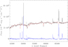 |
Fig. 1. Example of subtraction of the stellar emission from the MUSE spectra. The black line is the spectrum extracted at the continuum peak, the red line is the best fit stellar continuum, the blue line represents the residuals after continuum subtraction showing the emission lines. |
We then fitted the brightest emission lines (namely, Hβ, [O III]λλ4959,5007, [O I]λλ6300,6363, Hα, [N II]λλ6548,6584, and [S II]λλ6716,6731) in the continuum-subtracted spectra. We assumed that the lines in the red and blue portion of the spectra have the same velocity profile. While a single Gaussian reproduces the lines profiles at large radii accurately, in the nuclear regions (i.e., within 2″ from the galaxy center), we included an additional Gaussian component. In the following figures, we only show the results for the spaxels in which the line of interest is detected at a 2σ level at least.
We re-reduced 1981 March L band, A-configuration VLA observations of 3C 277.3 that were originally published in van Breugel et al. (1985). Data reduction was carried out in CASA version 5.6.2-3, and the original uvfits files were imported to a measurement set using the task importvla. Standard calibration was applied, with 3C286 serving as the flux calibrator and 3C287 as the phase calibrator. Imaging deconvolution was accomplished with the task clean, where we used a multi-scale clean including elements with a scale of 0, 5, 25, and 100 pixels. We used Briggs weighting with a robust parameter of 0.5. The final image has a pixel scale of  and an rms of 0.28 mJy beam−1 at 1.41 GHz. The synthesized beam is
  , and the peak flux is 17 mJy beam−1 for the radio core.
3. Results
In Fig. 2 we show the distribution of the Hα line emission. The radio contours are superposed. As already found previously (Miley et al. 1981; Tadhunter et al. 2000), a nebula of ionized gas with a size of ∼90 kpc × 60 kpc enshrouds the radio emission. The brightest emission line regions are located along the radio axis (at a position angle ∼ − 25°), while a series of narrow filaments follows the edges of the radio structure.
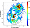 |
Fig. 2. Distribution of the Hα line emission where this is detected at a 2σ level at least in single spaxels. The radio contours at 1.41 GHz are superposed. The lowest isocontour is at 0.9 mJy beam−1. The contours then follow a geometric progression with a common ratio of 2. |
In Fig. 3 we show an image of the ratio of the high-ionization line [O III] with respect to the Hα intensity1 to study the ionization structure within the nebula. This image shows the presence of a biconical region characterized by a high [O III]/Hα ratio (as high as ∼7), with a sharp transition to significantly lower ratios in the outward regions. By defining the bicone to include the regions in which [O III]/Hα > 2.5, we obtain an axis at ∼ − 30° and an opening angle of ∼18°. The adopted threshold is somewhat arbitrary, but given the steep gradient in the [O III]/Hα ratio, values between 1.5 and 3.5 return similar values and suggest a rather small uncertainty in the cone size, ∼5°.
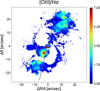 |
Fig. 3. Ratio of the [O III] and Hα lines where both lines are detected above a 2σ level. The gray lines mark the boundary of the high-ionization bicone, i.e., the regions in which [O III]/Hα > 2.5. |
3.1. Gas ionization mechanism
Spectroscopic diagnostic diagrams are commonly used to identify the gas ionization mechanism (e.g., Heckman 1980; Baldwin et al. 1981; Veilleux & Osterbrock 1987; Kewley et al. 2006; Law et al. 2021). The three diagrams are defined by four emission line ratios ([O III]/Hβ versus [N II]/Hα, [S II]/Hα, and [O I]/Hα) that are sensitive to the gas ionization properties. They allow us to identify the ionization mechanism because gas ionized by star-forming regions and by AGN fall into different regions of these diagrams. In Fig. 4 we show three images that are color-coded to identify individual spaxels falling into the area of star-forming galaxies (blue) and AGN, separating between high- and low-excitation galaxies (HEGs in red and LEGs in green, respectively). Intermediate objects are shown in orange, according to the regions defined by Law et al. (2021). These images are defined at the locations in which all four emission lines we considered reach a 2σ level in single spaxels. They show a very complex ionization structure: a biconical region, aligned with the radio axis, has a spectrum typical of HEGs, and it is surrounded by filaments of lower ionization and regions with spectra of star-forming regions.
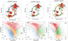 |
Fig. 4. Images obtained by color-coding the emission line regions depending on the location of the representative points in the diagnostic diagrams. Red shows high-excitation regions, green shows low-excitation regions, blue shows star-forming regions, and orange represents intermediate objects using the regions from Law et al. (2021). The images are defined where all four emission lines considered reach a 2σ level in a single spaxel. The gray lines mark the boundary of the high-ionization bicone. |
To explore the ionization properties in more detail and explore regions of low surface brightness that are not properly sampled by the single-spaxel analysis, we need to increase the S/N. We therefore extracted spectra over circles with a radius of  at the 76 locations marked in Fig. 5. We computed the emission line intensity ratios for all regions. The lines S/N is sufficient (i.e., > 3 for all lines) to locate 63 of them (Fig. 7). In Fig. 6 we show the spectra of four representative regions. In the appendix, we list the position and line ratios for these regions.
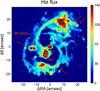 |
Fig. 5. Hα image of Coma A showing the regions in which this line is detected at a 2σ level at least in single spaxels. We mark the locations from which we extracted the spectra (empty circles). We identify with red arrows the five compact knots of star formation and also mark the location of the radio knots K1 and K2. The gray lines mark the boundary of the high-ionization bicone. The color bar shown on the right side is in units of 10−18 erg s−1 cm−2 arcsec−2. |
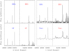 |
Fig. 6. Blue and red spectra of four representative regions. |
We identified five compact knots of line emission (marked in Fig. 7 with blue and cyan circles) whose representative points fall in the region of star-forming (SF) galaxies in all three diagnostic diagrams. The two brightest knots are located east of the nucleus, at a projected distance of ∼15″ (∼25 kpc). The other three are instead part of the large-scale filaments visible in the NW and SW: the most distant of them is ∼35″ (∼60 kpc) NW of the host galaxy. The brightest SF knot has a full width at half maximum that is consistent with the seeing of the observations. The other four knots are superposed on diffuse emission, and their sizes cannot be measured accurately.
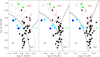 |
Fig. 7. Location of the selected regions in the spectroscopic diagnostic diagrams. Filled black dots correspond to regions outside the high-ionization bicone, and the red empty dots are the regions inside the bicone (the nucleus is identified with an additional blue diamond). The five large dots correspond to the compact knots of star formation (the cyan dots are the three knots in the outer filaments). The green squares are associated with radio knots K1 and K2. The solid curves separate SF from intermediate galaxies (Int.), and the dotted curve separates intermediate galaxies from AGN. The black lines separate LEGs and HEGS (Law et al. 2021). |
The line ratios, in particular, the N2 ratios (−0.85 < log[N II]/Hα < −0.6), are indicative of a subsolar gas metallicity, Z ∼ 0.6 − 0.8 Z⊙ (Pettini & Pagel 2004). The age of the stars can instead be constrained from the equivalent width of the Balmer lines (Leitherer et al. 1999). For the brightest SF knot, we measured an EWHβ = 80 ± 3 Å, corresponding to an age of ∼3 × 10⁶ years for an instantaneous burst of star formation. As discussed in detail below, an instantaneous burst is the most likely scenario in this source.
We estimated the effects of dust absorption by measuring the Hα/Hβ ratio in each region, adopting the Cardelli et al. (1989) law and RV = 3.1. The median value is E(B − V)∼0.1 (with a range 0.05 ≲ E(B − V)≲0.2), which is larger than the Galactic value of ∼0.01. This is indicative of significant internal reddening. There is no clear structure in the gas reddening, nor a connection between the reddening value and structures observed in the emission line flux maps.
We estimated the star formation rate (SFR) by measuring the Hα luminosity produced by the five SF knots. The resulting Hα luminosity, corrected for reddening, is ∼5.4 × 1040 erg s−1. The corresponding SFR is ∼0.8 M⊙ y−1. The dominant source of uncertainty for this estimate, a factor 3, is related to the adopted initial mass function of the stellar population (Pflamm-Altenburg et al. 2007).
The spectra of the majority of the selected locations within the high-ionization bicone are characteristic of HEGs, the same behavior as in the nucleus of Coma A. Regions with a higher [O III]/Hα ratio are aligned with the radio axis, but do not follow the curvature of the radio source, in particular, in the south lobe. This suggests that in this region, the main ionization mechanism is photoionization from the nuclear radiation field, and it is not related to the jets.
The regions outside the bicone show a complex behavior. In the first and second diagnostic plots, they are mainly located in places in which the line ratios correspond to those in SF galaxies (Law et al. 2021). Some regions straddle the separation line between SF galaxies and intermediate galaxies. This is suggestive of a mixed contribution of star formation and AGN. However, in the third diagram, they fully enter into the region of LEGs. This suggests that photoionization, either by young stars or by an AGN, does not account for the general location of the representative points of the filamentary emission line regions in Coma A.
Several alternative gas ionization mechanisms other than photoionization have been proposed: ionization due to hot cooling gas (Voit et al. 1994), thermal conduction within the intracluster medium (McDonald et al. 2010), reconnection diffusion (Fabian et al. 2011), and fast ionizing shocks (Dopita & Sutherland 1995; Allen et al. 2008). Only the shock models produce an excitation state that is characterized by an [O III]/Hβ ratio as high as that measured in the emission line filaments in Coma A.
We then focused on the MAPPINGS III library of shock models by Allen et al. (2008). We considered models of various metallicity, density, and magnetic field. The model that best reproduces the observations, that is, the model whose track follows the distribution of the measured line ratios more closely, is shown in Fig. 8. It corresponds to a twice solar metallicity, a gas density of 1 cm−3, and a no magnetic field. Overall, the predicted line ratios cover the range of the observed values with shock velocities in the range 350−500 km s−1.
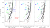 |
Fig. 8. Comparison between the predictions from models of ionization from fast shocks (Allen et al. 2008) and observed line ratios, limited to the regions outside the high-ionization bicone. The black curve shows the line ratios for a gas density of 1 cm−3, a metallicity Z = 2 × Z⊙, and a null magnetic field. The shock velocity ranges from 200 to 1000 km s−1 in steps of 25 km s−1, starting from the bottom left corner. The thick portion of the curve corresponds to the range vs = 350 − 500 km s−1. The dotted red lines are models with a magnetic field of 0.5 μG and Z = 2 × Z⊙. The green (dashed) and blue (dot-dashed) curves are the tracks obtained for a solar metallicity and B = 0 μG and B = 0.5 μG, respectively. The five large dots (coded as in Fig. 3) correspond to the compact knots of star formation (the cyan dots are the three knots in the outer filaments). |
The dependence of the line ratios on the various parameters is strong. For example, for a magnetic field of 0.5 μG, the diagnostic tracks (the dotted red curves in Fig. 8) move toward the bottom right corners of the diagrams and do not reproduce the measured ratios. Similarly, the tracks obtained for a solar metallicity (the green and blue curves in Fig. 8) overlap the observed values only marginally.
Finally, we estimated the density of the ionized gas by measuring the [S II]λ6716/[S II]λ6731 ratio (Osterbrock 1989). Considering the errors (whose median value is 0.12), this ratio is always higher than 1.3. This is indicative of a general low gas density (ne < 100 cm−3).
3.2. Emission lines at the radio knots K1 and K2
At a distance of ∼6″ (∼10 kpc) from the nucleus, the southern jet bends by ∼40°. At this location lie two bright knots of radio emission (labeled K1 and K2 in van Breugel et al. 1985). Emission lines associated with these knots were first reported by Miley et al. (1981), and nonthermal X-ray emission is seen in the Chandra images (Worrall et al. 2016). The HST broadband images (Martel et al. 1999) show a narrow filament oriented along a NS direction, and a similar morphology is seen in the [O III] image (Tilak et al. 2005). The emission line MUSE images also present an elongated structure, but it is more extended, ∼5″, than that seen by HST (∼2″ long).
The emission line ratios from the MUSE data for the two knots (represented by the green squares in Fig. 7) are similar to those measured in the surrounding regions. The comparison with the MAPPINGS III tracks does not return any shock model predicting the observed ratios. These results suggest that despite the in situ ionizing continuum seen in both the optical and X-ray images, the dominant ionization mechanism in this region is due to the nuclear radiation field.
3.3. Gas kinematics
Figure 9 presents the velocity field of the ionized gas and the distribution of line widths, not corrected for the instrumental resolution (∼50 km s−1 at the Hα wavelength, e.g., Guérou et al. 2017). The velocities are referred to the redshift measured (z = 0.08566) in the nuclear spectrum from the stellar absorption lines. The southern emission line lobe (associated with the approaching radio jet) has a rather constant blueshifted velocity of ∼100 km s−1 with small fluctuations, the most notable being the region immediately west of the radio knots K1 and K2, where a redshift of ∼30 km s−1 is observed. The northern lobe is instead generally redshifted, but it shows a more complex velocity structure than the southern lobe. The NE filament shows a redshift of ∼150 km s−1. Isolated blueshifted regions are also seen and are apparently connected with the extension of filaments located in the southern lobe. The highest velocities are reached beyond the edge of the northern radio lobe, with velocities exceeding ∼300 km s−1. Overall, the line widths (not corrected for instrumental resolution) are between 100 and 150 km s−1. The velocity dispersion reaches its maximum (≳400 km s−1) in two regions, at the southern tip of the nebula, close to where the radio hot spot is located, and the other ∼1″ − 2″ just west of the K1 and K2 knot. It is interesting that the region with the highest velocity dispersion is not coincident with the location of the radio and line knots, but is offset from it by a few kiloparsec. The lowest velocity widths (consistent with the MUSE spectral resolution) are seen in the regions with the highest velocities beyond the end of the northern lobe.
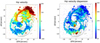 |
Fig. 9. Velocity field (left) and velocity dispersion (not corrected for instrumental resolution, right), both in km s−1, of the ionized gas derived from the Hα emission line. We superposed the radio contours in both panels. Contours are drawn starting from 0.9 mJy beam−1 with geometric progression with a common ratio of 2. |
4. Discussion
From the analysis of the emission line ratios, we found evidence for photoionization from young stars at five locations within the gas nebula surrounding the radio emission in Coma A. As discussed by Mellema et al. (2002), a cloud overtaken by shocks breaks up into dense fragments that are Jeans unstable, and might form stars. It then appears that the shocks produced by the expansion of the radio lobes are causing the formation of new stars. Star formation requires the presence of dense clouds of cold gas. Morganti et al. (2002) reported the detection of neutral hydrogen seen in absorption with a total mass of at least 109 M⊙ at distances as large as ∼30 kpc from the center. Coma A is the only radio galaxy in which H I is seen in absorption at such large distances from the nucleus. Furthermore, Morganti et al. (2002) suggested that the neutral hydrogen and ionized gas, based on their similar kinematics, are part of the same structure, possibly the remnant of a gas-rich merger.
Alternatively, the formation of molecular clouds can be due to thermal instabilities that are causing the rapid cooling of gas that is outflowing from the nucleus (Zubovas & King 2014): a two-phase medium forms, with cold dense molecular clumps mixed with hot tenuous gas, leading to star formation. The situation in Coma A is somewhat different from that envisaged by these authors because its outflow is probably dominated by relativistic plasma, not by thermal gas. However, an outflow of denser gas might be induced by a snow-plowing effect along the edges of the radio source.
For the remaining regions (outside the high-ionization bicone, marked as black dots in Figs. 7 and 8) models of ionization from fast shocks with velocities of 350−500 km s−1 are able to reproduce the overall range of the measured emission line ratios. Despite the reasonably good agreement between the model predictions and the observations, the required metallicity value is higher than what we found for the SF knots. Furthermore, such a high metal content for gas located at such large distances from the center of the host galaxy appears to be rather contrived.
The detection of SF knots, in particular, those located along the western filaments at the edges of the radio lobe, suggests that we might be seeing the combined effect of shocks and young stars. Gas ionized by the two processes is present within a given integration region, leading to the observed line ratios. A similar mechanism of star formation within a turbulent flow has been suggested by McDonald et al. (2012) to account for the emission line ratios observed in the gaseous filaments of cool-core galaxy clusters.
The possibility of diffuse star formation within the filaments suggests that the SFR value estimated above for the five star-forming knots should be considered a lower limit. The total Hα luminosity outside the bicone is three times higher than that measured in the SF knots alone. In addition, SF might occur also within the high-ionization bicone. However, the IRAS satellite failed to detect Coma A: the upper limits in the 60 and 100 μm can be used to estimate a limit to the total far-IR luminosity of LFIR < 2.5 × 10¹⁰ L⊙ (Ocaña Flaquer et al. 2010), and finally, using the relation by Gao & Solomon (2004), a limit to the star formation rate of about < 5 M⊙ yr−1.
Previous studies of RGs show that these sources span a large range of SFR, beginning at the galaxy main sequence, but they are often found among the passive galaxies with very low SFRs (Dabhade et al. 2020; Bernhard et al. 2021). The stellar mass of Coma A can be estimated by using its K-band luminosity and the correlation from Cappellari (2013), resulting in M* = 3.3 × 10¹¹ M⊙. When combined with the estimate of the SFR, this value locates Coma A well within the galaxy main sequence (Saintonge et al. 2017). The key difference lies in the result that in Coma A, the star formation occurs well outside the host galaxy, at distances as large as 60 kpc.
The sharp edges of the radio lobes of 3C 277.3 indicate that they are at a higher pressure than the external medium. The expansion of an overpressured cocoon occurs at a supersonic speed  , where Pc and Pem are the pressure of the radio cocoon and of the external medium, respectively (Begelman & Cioffi 1989). The sound speed of the external medium, cs, for a temperature of 1 keV estimated from X-ray images (Worrall et al. 2016) is ∼500 km s−1. We can set an upper limit to the time τexp. in which the angular size of the radio source grows by
  , for instance (the resolution of the MUSE data, corresponding to dl = 800 pc), τexp. = dl/vexp. < 1.6 × 10⁶ years. This timescale implies that we are effectively seeing an instantaneous burst of star formation.
The expanding radio-emitting plasma also plays a role for the kinematics of the ionized gas. As described above, the gas velocity field is quite complex, and although it shows a general symmetry, it is not compatible with gas in ordered rotation. At various locations (e.g., immediately west of radio knots K1 and K2 and at the southern radio hot spot), we found a connection between radio and optical emission, with a strong increase in gas velocity dispersion that bears witness to the effects of jet and cloud interactions. The opposite behavior is seen in the region at the northern tip of the ionized nebula, which is the only location in which gas is detected outside the radio cocoon. Here, the gas has a small velocity gradient and produces line emission with a very small width. This indicates that it is unperturbed. However, if the expansion of the lobes were the dominant driver of the gas kinematics and this occurred within a gas structure encompassing the whole radio structure, we would expect to see a quite different velocity field: the two lobes should each induce the expansion of a gas bubble, with a blueshifted and a redshifted component on either side. The observed kinematics can be reconciled with a dominance of the radio outflows if the gas has a flattened disk structure and if the jets are oriented so that they graze the gas disk: in this case, only one side of the lobe would interact with the denser gas regions, producing the observed asymmetry. Alternatively, the gas dynamics is dominated by gravity and the radio outflow only produces localized disturbances, or the complex velocity field is due to the external (merger) origin of the gas that has not yet reached a dynamical equilibrium.
The brightest regions of line emission in Coma A are located within a biconical region in which we also find the highest [O III]/Hα ratios. This morphology is reminiscent of what is often observed in type 2 Seyfert galaxies (e.g., Tadhunter & Tsvetanov 1989), and it is indicative of circumnuclear selective obscuration, as postulated by the unified model (UM) of AGN (Antonucci 1993). The lack of broad lines in Coma A (Buttiglione et al. 2010) and the high column density derived from the nuclear X-ray spectrum (Worrall et al. 2016; Macconi et al. 2020) are in line with the idea that our view toward its nucleus intercepts regions of high absorption. However, the angular size of the bicone is smaller (∼18° ±5°) than predicted by the UM estimate: based on the relative number of 3CR RGs with z < 0.3 with and without broad lines in their optical spectra. Baldi et al. (2013) estimated that this fraction corresponds to an average cone aperture of ∼50 ± 5°. This discrepancy might be due to the combination of an intrinsic anisotropy of the nuclear radiation field and additional ionization mechanisms. In this case, the relative contribution of the AGN light is reduced at larger angles from the disk axis. The nuclear anisotropy might be due to the geometrical thickness of the accretion disk (e.g., Sikora & Wilson 1981), but also to a contribution to the radiation field from relativistically beamed emission from the jet base. While in blazars, this collimated beam points at a small angle from the line of sight, in radio galaxies such as Coma A, it would illuminate a biconical region with an opening angle θ ∼ Γ−1, where Γ is the jet Lorentz factor.
5. Summary and conclusions
We presented the results of VLT/MUSE observations of the nearby radio galaxy Coma A that show a large nebula (∼90 kpc × 60 kpc) of ionized gas cospatial with the radio emission. We estimated the emission line ratios in several regions throughout the nebula to explore the gas ionization mechanism. Five compact knots have line ratios that are indicative of ionization from young stars with an estimated age of ∼3 × 10⁶ years and a subsolar gas metallicity, Z ∼ 0.6 − 0.8 Z⊙.
Three star-forming regions (detected as far as 60 kpc from the host) are part of the gas filaments surrounding the western edges of the radio lobes. The most likely origin of these filaments is the compression of the ambient gas produced by the expanding radio source that increases its density, boosting the line emission. This same compression causes the collapse of the gas clouds, leading to the formation of new stars. The two brightest SF knots are instead located at a projected distance of 25 kpc east of the center of the galaxy, within a channel of lower radio surface brightness between the two lobes. In this region, the compression might be due to the plasma flowing back from the radio spots. There is not necessarily a causal connection between the radio ejecta and the star formation event at this location: star-forming knots are commonly associated with gas-rich merger events, the most likely explanation for the large amount of gas in Coma A.
A reservoir of dense gas is needed to maintain star formation. Cold gas is indeed detected in Coma A from its HI absorption against the radio continuum extending to a very large radius, at least ∼30 kpc. In this context, it would be of great interest to derive the distribution and kinematics of the molecular gas and its connection with the radio-emitting and ionized gas. The clumps of star formation found at ∼40−60 kpc from the center of the galaxy suggest that the molecular gas should extend to these large distances. Its distribution would enable us to test whether it survives within the radio lobes or is destroyed by shock heating, ultimately quenching future star formation.
In addition to the star-forming regions, the gas nebula around Coma A shows a well-defined ionization structure. Within a narrow bicone, with an opening angle of ∼18°, the gas is in a high-ionization state. The relatively small angle of the bicone (with respect to the indications of the AGN unification scheme) suggests that this is not solely due to circumnuclear obscuration, but that an intrinsic anisotropy of the nuclear radiation field is present. This might be due to effects of radiative transport within a thick accretion disk, but there is also the possibility that we are seeing the result of relativistic beaming, that is, that a blazar nucleus, oriented at a large angle from our line of sight, is present in this radio source.
Outside the high-ionization bicone, the gas is in a much lower ionization state. The location in the diagnostic diagrams does not follow the distribution of photoionized gas from either an active nucleus or young stars, suggesting an additional ionization mechanism. Shocks with a velocity of 350−500 km s−1 produce line ratios similar to the observed ratios, but with preferred values of null magnetic field and a twice solar gas metallicity. These values contradict the measurements based on the Faraday rotation (∼1 μG) and with the metallicity estimated on the SF knots. This suggests a contribution from diffuse star formation produced within the ionized gas filaments. UV imaging represents the best tool to separate the contribution of SF and shocks to the gas ionization budget because as shown by McDonald et al. (2011), the ratio between line and UV continuum emission is radically different in these two scenarios. UV images would also enable us to map the distribution and estimate the age of young stars, and to follow the star formation history in this galaxy. Given the high advancing speed of the radio lobes, they might leave a resolved trail of star-forming regions of increasing age when they move toward the nucleus.
In low-redshift RGs with evidence of star formation triggered by the jets discussed in the Introduction, young stars are formed in a few locations along the path or at the termination of a radio jet. In these objects, the SFR is generally lower than our conservative estimate for Coma A (∼0.8 M⊙ y−1): 1 × 10⁻³ − 5 × 10⁻³ M⊙ y−1 in Centaurus A (Salomé et al. 2016), and 0.5, and 0.03 for the Minkowski object, and NGC 5643, respectively. However, the main distinguishing feature in this source is that the line ratios suggest that star formation, clearly detected in a few individual knots, occurs throughout the whole gaseous structure that enshrouds the whole radio source at distances as large as 60 kpc. In this sense, Coma A might be a unique source in the local Universe in which the expanding radio source appears to be triggering a global event of star formation. This represents an excellent laboratory for exploring the mechanism of positive feedback in detail.
We preferred to produce the [O III]/Hα map instead of the reddening -independent [O III]/Hβ image because Hβ is detected at a sufficient S/N level over a much smaller area.
Acknowledgments
Based on observations collected at the European Southern Observatory under ESO program 0102.B-0048(A). S.B. and C.O.D. are grateful to the Natural Sciences and Engineering Research Council (NSERC) of Canada. R.G. acknowledges support from the agreement ASI-INAF n. 2017-14-H.O. G.V. acknowledges support from ANID program FONDECYT Postdoctorado 3200802.
References
- Allen, M. G., Groves, B. A., Dopita, M. A., Sutherland, R. S., & Kewley, L. J. 2008, ApJS, 178, 20 [Google Scholar]
- Antonucci, R. 1993, ARA&A, 31, 473 [Google Scholar]
- Baldi, R. D., Capetti, A., Buttiglione, S., Chiaberge, M., & Celotti, A. 2013, A&A, 560, A81 [NASA ADS] [CrossRef] [EDP Sciences] [Google Scholar]
- Baldwin, J. A., Phillips, M. M., & Terlevich, R. 1981, PASP, 93, 5 [Google Scholar]
- Balmaverde, B., Capetti, A., Marconi, A., et al. 2019, A&A, 632, A124 [NASA ADS] [CrossRef] [EDP Sciences] [Google Scholar]
- Balmaverde, B., Capetti, A., Marconi, A., et al. 2021, A&A, 645, A12 [EDP Sciences] [Google Scholar]
- Begelman, M. C., & Cioffi, D. F. 1989, ApJ, 345, L21 [CrossRef] [Google Scholar]
- Bennett, C. L., Larson, D., Weiland, J. L., & Hinshaw, G. 2014, ApJ, 794, 135 [Google Scholar]
- Bernhard, E., Tadhunter, C., Mullaney, J. R., et al. 2021, MNRAS, 503, 2598 [NASA ADS] [CrossRef] [Google Scholar]
- Bîrzan, L., Rafferty, D. A., Nulsen, P. E. J., et al. 2012, MNRAS, 427, 3468 [Google Scholar]
- Buttiglione, S., Capetti, A., Celotti, A., et al. 2010, A&A, 509, A6 [NASA ADS] [CrossRef] [EDP Sciences] [Google Scholar]
- Capetti, A., de Ruiter, H. R., Fanti, R., et al. 2000, A&A, 362, 871 [NASA ADS] [Google Scholar]
- Cappellari, M. 2013, ApJ, 778, L2 [NASA ADS] [CrossRef] [Google Scholar]
- Cappellari, M., & Copin, Y. 2003, MNRAS, 342, 345 [Google Scholar]
- Cappellari, M., & Emsellem, E. 2004, PASP, 116, 138 [Google Scholar]
- Cardelli, J. A., Clayton, G. C., & Mathis, J. S. 1989, ApJ, 345, 245 [Google Scholar]
- Cresci, G., Marconi, A., Zibetti, S., et al. 2015, A&A, 582, A63 [NASA ADS] [CrossRef] [EDP Sciences] [Google Scholar]
- Crockett, R. M., Shabala, S. S., Kaviraj, S., et al. 2012, MNRAS, 421, 1603 [NASA ADS] [CrossRef] [Google Scholar]
- Croft, S., van Breugel, W., de Vries, W., et al. 2006, ApJ, 647, 1040 [NASA ADS] [CrossRef] [Google Scholar]
- Dabhade, P., Combes, F., Salomé, P., Bagchi, J., & Mahato, M. 2020, A&A, 643, A111 [NASA ADS] [CrossRef] [EDP Sciences] [Google Scholar]
- Dopita, M. A., & Sutherland, R. S. 1995, ApJ, 455, 468 [Google Scholar]
- Drouart, G., De Breuck, C., Vernet, J., et al. 2014, A&A, 566, A53 [NASA ADS] [CrossRef] [EDP Sciences] [Google Scholar]
- Fabian, A. C., Sanders, J. S., Williams, R. J. R., et al. 2011, MNRAS, 417, 172 [NASA ADS] [CrossRef] [Google Scholar]
- Gao, Y., & Solomon, P. M. 2004, ApJ, 606, 271 [NASA ADS] [CrossRef] [Google Scholar]
- Garrington, S. T., Leahy, J. P., Conway, R. G., & Laing, R. A. 1988, Nature, 331, 147 [Google Scholar]
- Gilli, R., Mignoli, M., Peca, A., et al. 2019, A&A, 632, A26 [NASA ADS] [CrossRef] [EDP Sciences] [Google Scholar]
- Guérou, A., Krajnović, D., Epinat, B., et al. 2017, A&A, 608, A5 [Google Scholar]
- Gültekin, K., Richstone, D. O., Gebhardt, K., et al. 2009, ApJ, 698, 198 [Google Scholar]
- Hardcastle, M. J., & Croston, J. H. 2020, New Astron. Rev., 88, 101539 [Google Scholar]
- Heckman, T. M. 1980, A&A, 87, 152 [Google Scholar]
- Kewley, L. J., Groves, B., Kauffmann, G., & Heckman, T. 2006, MNRAS, 372, 961 [Google Scholar]
- Knuettel, S., O’Sullivan, S. P., Curiel, S., & Emonts, B. H. C. 2019, MNRAS, 482, 4606 [NASA ADS] [CrossRef] [Google Scholar]
- Laing, R. A., & Peacock, J. A. 1980, MNRAS, 190, 903 [Google Scholar]
- Law, D. R., Belfiore, F., Ji, X., et al. 2021, ApJ, 915, 35 [NASA ADS] [CrossRef] [Google Scholar]
- Leitherer, C., Schaerer, D., Goldader, J. D., et al. 1999, ApJS, 123, 3 [Google Scholar]
- Macconi, D., Torresi, E., Grandi, P., Boccardi, B., & Vignali, C. 2020, MNRAS, 493, 4355 [NASA ADS] [CrossRef] [Google Scholar]
- Madrid, J. P., Chiaberge, M., Floyd, D., et al. 2006, ApJS, 164, 307 [NASA ADS] [CrossRef] [Google Scholar]
- Martel, A. R., Baum, S. A., Sparks, W. B., et al. 1999, ApJS, 122, 81 [NASA ADS] [CrossRef] [Google Scholar]
- McDonald, M., Veilleux, S., Rupke, D. S. N., & Mushotzky, R. 2010, ApJ, 721, 1262 [Google Scholar]
- McDonald, M., Veilleux, S., Rupke, D. S. N., Mushotzky, R., & Reynolds, C. 2011, ApJ, 734, 95 [CrossRef] [Google Scholar]
- McDonald, M., Veilleux, S., & Rupke, D. S. N. 2012, ApJ, 746, 153 [Google Scholar]
- McNamara, B. R., & Nulsen, P. E. J. 2007, ARA&A, 45, 117 [NASA ADS] [CrossRef] [Google Scholar]
- Mellema, G., Kurk, J. D., & Röttgering, H. J. A. 2002, A&A, 395, L13 [NASA ADS] [CrossRef] [EDP Sciences] [Google Scholar]
- Miley, G., & De Breuck, C. 2008, A&ARv, 15, 67 [Google Scholar]
- Miley, G. K., Heckman, T. M., Butcher, H. R., & van Breugel, W. J. M. 1981, ApJ, 247, L5 [NASA ADS] [CrossRef] [Google Scholar]
- Morganti, R., Oosterloo, T. A., Tinti, S., et al. 2002, A&A, 387, 830 [NASA ADS] [CrossRef] [EDP Sciences] [Google Scholar]
- Mould, J. R., Ridgewell, A., Gallagher, J. S., III, et al. 2000, ApJ, 536, 266 [NASA ADS] [CrossRef] [Google Scholar]
- Neff, S. G., Eilek, J. A., & Owen, F. N. 2015, ApJ, 802, 88 [NASA ADS] [CrossRef] [Google Scholar]
- Ocaña Flaquer, B., Leon, S., Combes, F., & Lim, J. 2010, A&A, 518, A9 [Google Scholar]
- O’Dea, C. P., & Saikia, D. J. 2021, A&ARv, 29, 3 [Google Scholar]
- Osterbrock, D. E. 1989, Astrophysics of Gaseous Nebulae and Active Galactic Nuclei (Mill Valley: University Science Books) [Google Scholar]
- Pettini, M., & Pagel, B. E. J. 2004, MNRAS, 348, L59 [NASA ADS] [CrossRef] [Google Scholar]
- Pflamm-Altenburg, J., Weidner, C., & Kroupa, P. 2007, ApJ, 671, 1550 [NASA ADS] [CrossRef] [Google Scholar]
- Podigachoski, P., Barthel, P. D., Haas, M., et al. 2015, A&A, 575, A80 [NASA ADS] [CrossRef] [EDP Sciences] [Google Scholar]
- Rejkuba, M., Minniti, D., Courbin, F., & Silva, D. R. 2002, ApJ, 564, 688 [NASA ADS] [CrossRef] [Google Scholar]
- Saintonge, A., Catinella, B., Tacconi, L. J., et al. 2017, ApJS, 233, 22 [Google Scholar]
- Salomé, Q., Salomé, P., Combes, F., Hamer, S., & Heywood, I. 2016, A&A, 586, A45 [NASA ADS] [CrossRef] [EDP Sciences] [Google Scholar]
- Santoro, F., Oonk, J. B. R., Morganti, R., Oosterloo, T. A., & Tremblay, G. 2015, A&A, 575, L4 [NASA ADS] [CrossRef] [EDP Sciences] [Google Scholar]
- Sikora, M., & Wilson, D. B. 1981, MNRAS, 197, 529 [NASA ADS] [CrossRef] [Google Scholar]
- Solórzano-Iñarrea, C., & Tadhunter, C. N. 2003, MNRAS, 340, 705 [CrossRef] [Google Scholar]
- Steinbring, E. 2011, AJ, 142, 172 [CrossRef] [Google Scholar]
- Steinbring, E. 2014, AJ, 148, 10 [NASA ADS] [CrossRef] [Google Scholar]
- Tadhunter, C., & Tsvetanov, Z. 1989, Nature, 341, 422 [NASA ADS] [CrossRef] [Google Scholar]
- Tadhunter, C. N., Villar-Martin, M., Morganti, R., Bland-Hawthorn, J., & Axon, D. 2000, MNRAS, 314, 849 [NASA ADS] [CrossRef] [Google Scholar]
- Tilak, A., O’Dea, C. P., Tadhunter, C., et al. 2005, AJ, 130, 2513 [NASA ADS] [CrossRef] [Google Scholar]
- van Breugel, W., Miley, G., Heckman, T., Butcher, H., & Bridle, A. 1985, ApJ, 290, 496 [NASA ADS] [CrossRef] [Google Scholar]
- Vazdekis, A., Sánchez-Blázquez, P., Falcón-Barroso, J., et al. 2010, MNRAS, 404, 1639 [NASA ADS] [Google Scholar]
- Veilleux, S., & Osterbrock, D. E. 1987, ApJS, 63, 295 [Google Scholar]
- Voit, G. M., Donahue, M., & Slavin, J. D. 1994, ApJS, 95, 87 [Google Scholar]
- Weilbacher, P. M., Palsa, R., Streicher, O., et al. 2020, A&A, 641, A28 [NASA ADS] [CrossRef] [EDP Sciences] [Google Scholar]
- Worrall, D. M., Birkinshaw, M., & Young, A. J. 2016, MNRAS, 458, 174 [NASA ADS] [CrossRef] [Google Scholar]
- Zubovas, K., & King, A. R. 2014, MNRAS, 439, 400 [Google Scholar]
Appendix A: Emission line ratio measurements
Emission line ratio measurements.
All Tables
All Figures
|
Fig. 1. Example of subtraction of the stellar emission from the MUSE spectra. The black line is the spectrum extracted at the continuum peak, the red line is the best fit stellar continuum, the blue line represents the residuals after continuum subtraction showing the emission lines. |
| In the text | |
|
Fig. 2. Distribution of the Hα line emission where this is detected at a 2σ level at least in single spaxels. The radio contours at 1.41 GHz are superposed. The lowest isocontour is at 0.9 mJy beam−1. The contours then follow a geometric progression with a common ratio of 2. |
| In the text | |
|
Fig. 3. Ratio of the [O III] and Hα lines where both lines are detected above a 2σ level. The gray lines mark the boundary of the high-ionization bicone, i.e., the regions in which [O III]/Hα > 2.5. |
| In the text | |
|
Fig. 4. Images obtained by color-coding the emission line regions depending on the location of the representative points in the diagnostic diagrams. Red shows high-excitation regions, green shows low-excitation regions, blue shows star-forming regions, and orange represents intermediate objects using the regions from Law et al. (2021). The images are defined where all four emission lines considered reach a 2σ level in a single spaxel. The gray lines mark the boundary of the high-ionization bicone. |
| In the text | |
|
Fig. 5. Hα image of Coma A showing the regions in which this line is detected at a 2σ level at least in single spaxels. We mark the locations from which we extracted the spectra (empty circles). We identify with red arrows the five compact knots of star formation and also mark the location of the radio knots K1 and K2. The gray lines mark the boundary of the high-ionization bicone. The color bar shown on the right side is in units of 10−18 erg s−1 cm−2 arcsec−2. |
| In the text | |
|
Fig. 6. Blue and red spectra of four representative regions. |
| In the text | |
|
Fig. 7. Location of the selected regions in the spectroscopic diagnostic diagrams. Filled black dots correspond to regions outside the high-ionization bicone, and the red empty dots are the regions inside the bicone (the nucleus is identified with an additional blue diamond). The five large dots correspond to the compact knots of star formation (the cyan dots are the three knots in the outer filaments). The green squares are associated with radio knots K1 and K2. The solid curves separate SF from intermediate galaxies (Int.), and the dotted curve separates intermediate galaxies from AGN. The black lines separate LEGs and HEGS (Law et al. 2021). |
| In the text | |
|
Fig. 8. Comparison between the predictions from models of ionization from fast shocks (Allen et al. 2008) and observed line ratios, limited to the regions outside the high-ionization bicone. The black curve shows the line ratios for a gas density of 1 cm−3, a metallicity Z = 2 × Z⊙, and a null magnetic field. The shock velocity ranges from 200 to 1000 km s−1 in steps of 25 km s−1, starting from the bottom left corner. The thick portion of the curve corresponds to the range vs = 350 − 500 km s−1. The dotted red lines are models with a magnetic field of 0.5 μG and Z = 2 × Z⊙. The green (dashed) and blue (dot-dashed) curves are the tracks obtained for a solar metallicity and B = 0 μG and B = 0.5 μG, respectively. The five large dots (coded as in Fig. 3) correspond to the compact knots of star formation (the cyan dots are the three knots in the outer filaments). |
| In the text | |
|
Fig. 9. Velocity field (left) and velocity dispersion (not corrected for instrumental resolution, right), both in km s−1, of the ionized gas derived from the Hα emission line. We superposed the radio contours in both panels. Contours are drawn starting from 0.9 mJy beam−1 with geometric progression with a common ratio of 2. |
| In the text | |
Current usage metrics show cumulative count of Article Views (full-text article views including HTML views, PDF and ePub downloads, according to the available data) and Abstracts Views on Vision4Press platform.
Data correspond to usage on the plateform after 2015. The current usage metrics is available 48-96 hours after online publication and is updated daily on week days.
Initial download of the metrics may take a while.