| Issue |
A&A
Volume 657, January 2022
|
|
|---|---|---|
| Article Number | A49 | |
| Number of page(s) | 19 | |
| Section | Astrophysical processes | |
| DOI | https://doi.org/10.1051/0004-6361/202141295 | |
| Published online | 05 January 2022 | |
Exploring the physics behind the non-thermal emission from star-forming galaxies detected in γ rays
1
Instituto Argentino de Radioastronomía, CONICET-CICPBA-UNLP, CC5 (1897) Villa Elisa, Prov. de Buenos Aires, Argentina
e-mail: This email address is being protected from spambots. You need JavaScript enabled to view it.
2
Niels Bohr International Academy, Niels Bohr Institute, University of Copenhagen, Blegdamsvej 17, 2100 Copenhagen, Denmark
3
Instituto de Astronomía y Física del Espacio, CONICET-UBA, C.C. 67, Suc. 28, 1428 Buenos Aires, Argentina
Received:
12
May
2021
Accepted:
18
September
2021
Abstract
Context. Star-forming galaxies emit non-thermal radiation from radio to γ rays. Observations show that their radio and γ-ray luminosities scale with their star formation rates, supporting the hypothesis that non-thermal radiation is emitted by cosmic rays produced by their stellar populations. However, the nature of the main cosmic-ray transport processes that shape the emission in these galaxies is still poorly understood, especially at low star formation rates.
Aims. Our aim is to investigate the main mechanisms of global cosmic-ray transport and cooling in star-forming galaxies. The way they contribute to shaping the relations between non-thermal luminosities and star formation rates could shed light onto their nature, and allow us to quantify their relative importance at different star formation rates.
Methods. We developed a model to compute the cosmic-ray populations of star-forming galaxies, taking into account their production, transport, and cooling. The model is parametrised only through global galaxy properties, and describes the non-thermal emission in radio (at 1.4 GHz and 150 MHz) and γ rays (in the 0.1−100 GeV band). We focused on the role of diffusive and advective transport by galactic winds, either driven by turbulent or thermal instabilities. We compared model predictions to observations, for which we compiled a homogeneous set of luminosities in these radio bands, and updated those available in γ rays.
Results. Our model reproduces reasonably well the observed relations between the γ-ray or 1.4 GHz radio luminosities and the star formation rate, assuming a single power-law scaling of the magnetic field (with index β = 0.3) and winds blowing either at Alfvenic speeds (∼tens of km s−1, for ≲5 M⊙ yr−1) or typical starburst wind velocities (∼hundreds of km s−1, for ≳5 M⊙ yr−1). Escape of cosmic rays is negligible for ≳30 M⊙ yr−1. A constant ionisation fraction of the interstellar medium fails to reproduce the 150 MHz radio luminosity throughout the whole star formation rate range.
Conclusions. Our results reinforce the idea that galaxies with high star formation rates are cosmic-ray calorimeters, and that the main mechanism driving proton escape is diffusion, whereas electron escape also proceeds via wind advection. They also suggest that these winds should be cosmic-ray or thermally driven at low and intermediate star formation rates, respectively. Our results globally support that magneto-hydrodynamic turbulence is responsible for the dependence of the magnetic field strength on the star formation rate and that the ionisation fraction is strongly disfavoured to be constant throughout the whole range of star formation rates.
Key words: galaxies: starburst / galaxies: star formation / gamma rays: galaxies / radio continuum: galaxies
© ESO 2022
1. Introduction
Star-forming galaxies (SFGs) are one of the extragalactic γ-ray source classes detected at gigaelectronvolt (GeV) energies by the Fermi-LAT telescope (Abdo et al. 2010a,b; Lenain et al. 2010; Ackermann et al. 2012). Their emission is believed to be associated with young stellar populations, which explains its correlation with star formation rate (SFR). In particular, γ rays are thought to be mostly produced in interactions between hadronic cosmic rays (CRs) with particles of the interstellar medium (ISM), while CRs are accelerated at supernova remnant (SNR) shocks (Jokipii & Morfill 1985; Blasi 2013; Bustard et al. 2017). In addition to SNRs, other sources related to star-forming regions, such as young massive star clusters or microquasars, could also play an important role in CR acceleration, possibly up to petaelectronvolt (PeV) energies (see e.g. Bykov & Toptygin 2001; Aharonian et al. 2019; Bykov et al. 2020; Escobar et al. 2021; Morlino et al. 2021). These acceleration sites are abundant in SFGs and are expected to be more numerous in sources with higher SFRs. Similarly, higher gas densities are found in higher SFR environments since the gas is the seed of star formation. As a result, an increase in the γ-ray emission is expected for higher star formation rates.
The main evidence supporting this interpretation is the observed correlation between the integrated γ-ray luminosity (Lγ) of SFGs and their SFRs (Ackermann et al. 2012; Ajello et al. 2020). The latter, in particular, is typically estimated from tracers such as the total infrared (IR) luminosity (LIR, 8 − 1000 μm). This relation was predicted by Thompson et al. (2007) and Lacki et al. (2010) in terms of the γ-ray flux and the gas surface density of SFGs. Several works have endeavoured to explain the high-energy emission of these objects individually (e.g. Völk et al. 1996; Blom et al. 1999; Romero & Torres 2003; Domingo-Santamaría & Torres 2005; de Cea del Pozo et al. 2009; Persic & Rephaeli 2010; Lacki et al. 2011; Rephaeli & Persic 2014; Krumholz et al. 2020) and others as a result of the common properties of the population of SFGs (e.g. Lacki et al. 2010; Pfrommer et al. 2017; Zhang et al. 2019; Peretti et al. 2020; Kornecki et al. 2020). There is a general consensus on the increasing dynamical relevance of radiative energy losses for higher SFRs, so that the CR transport in these environments is inferred to approach the calorimetric limit; specifically, all injected particles cool before being able to escape. In particular, while electron calorimetry is believed to be reached already in mild starbursts, SFR ≳ 5 M⊙ yr−1, the SFR range where proton calorimetry might be achieved is still under debate due to our current poor knowledge of the escape mechanisms.
Star forming galaxies have been observed and modelled throughout the whole electromagnetic spectrum (e.g. Völk et al. 1996; Persic & Rephaeli 2002, 2014; Persic et al. 2008; de Cea del Pozo et al. 2009; Rephaeli et al. 2010; Yoast-Hull et al. 2013; Peretti et al. 2019). Diffuse thermal and non-thermal emission from these objects has been observed in radio frequencies (e.g. Condon 1992; Cox et al. 1988; Loiseau et al. 1987; Strickland et al. 2002; Kapińska et al. 2017), X-rays (Bauer et al. 2008; Sarkar et al. 2016), and even very high-energy γ rays (Acciari et al. 2009; Acero et al. 2009).
Non-thermal radio and X-rays are produced by relativistic primary and secondary CR electrons, where primaries are injected together with protons at acceleration sites (see e.g. Cristofari et al. 2021; Aharonian et al. 2019 in the context of SNRs and star clusters, respectively) and secondaries are a by-product of the CR interaction with the ISM.
CR electrons in galactic magnetic fields (B) emit synchrotron radiation detectable mostly at radio frequencies. A connection between the synchrotron radiation and supernova rate was one of the first attempts to explain the linear correlation between the observed luminosity at 1.4 GHz (L1.4 GHz) and far-IR (FIR) luminosity (van der Kruit 1971; Condon 1992; Yun et al. 2001). However, the nature of this link is not trivial in low-SFR galaxies, due to their low efficiency in converting starlight into IR radiation, and the predominance of escape as the main driver of electron transport (Condon 1992; Yun et al. 2001; Bell 2003). This missing energy causes both radio and IR luminosities to underestimate the SFR for galaxies with low levels of IR emission. Bell (2003) argued that these two effects conspire to achieve a linear relation between IR luminosity and L1.4 GHz. At high SFRs the efficient cooling of protons typical of starburst galaxies (SBGs) leads to a copious production of secondary leptons whose synchrotron emission is inferred to overcome that of primaries (e.g. Torres 2004; Domingo-Santamaría & Torres 2005; Lacki et al. 2010). This could possibly impact the global shape of the correlation.
In addition to synchrotron processes, thermal processes such as free–free emission and absorption also characterise the radio emission of SFGs. Numerous young stars create several H II regions, whose hot ionised gas radiates thermally and contributes to the total radio emission. A spectral identification of such free–free emission is in general very complex due to the presence of other components such as synchrotron, dominating at GHz, and the FIR thermal peak produced by the dust, which occurs above a few tens of GHz. Many works have discussed the fraction of the thermal contribution in this band with respect to the non-thermal emission (e.g. Bell 2003; Klein et al. 2018). However, no definitive conclusion has been reached yet due to the complexity of this task.
Focusing on the synchrotron emission, many studies explored the SFR–luminosity correlation at lower radio frequencies, in particular at 150 MHz (e.g. Gürkan et al. 2018; Wang et al. 2019; Smith et al. 2021), where the free–free absorption might become severe. Typically, the free-free absorption significantly reduces the emission up to ∼10 − 102 MHz in galaxies with moderate SFRs (Schober et al. 2017; Chyży et al. 2018), and up to a few GHz in ultraluminous IR galaxies (ULIRGs; Condon et al. 1991; Clemens et al. 2010).
Although most of the radio emission is expected from CRs populating galactic discs, some additional radio emission produced in SFGs might have a different origin. In particular, a non-negligible contribution might come from individual sources such as SNRs (Lisenfeld & Völk 2000), activity of a coexisting active galactic nucleus (AGN; Mancuso et al. 2017), or particles populating the galactic halo as a consequence of the escape from the galactic disc via diffusion or advection in winds (Heesen et al. 2009; Romero et al. 2018). A smaller contribution of emission coming from pulsar wind nebulae (Ohm & Hinton 2013) and millisecond pulsars (Sudoh et al. 2021) is also possible; in particular, the latter can become important at low frequencies and low SFRs. Nevertheless, the contribution of these objects to the diffuse emission is still unclear.
Lacki et al. (2010) and Martin (2014) have explored the transport of CRs throughout the SFR range, studying at the same time both the radio and γ-ray correlations with SFR. This multiwavelength approach allowed better constraints on the role of CRs in shaping these correlations highlighting, in particular, the key role played by protons in the production of both γ rays and secondary electrons. The latter are inferred to be responsible for most of the radio emission at high SFRs, where protons are expected to be efficiently confined. Despite these recent improvements, our knowledge of the CR transport properties in SFGs remains poor and several questions are still open: How does the CR escape from galaxies evolve with the SFR and what is its impact on calorimetry? What is the interplay between primary and secondary electrons in shaping the radio luminosity of SFGs? Can the luminosity–SFR correlation help us explore possible dependences of magnetic and radiation fields in SFGs? What is the actual role and/or contamination of free–free emission and absorption in SFGs? Can it help us in exploring alternative cosmic acceleration sites?
In this work we address these issues by exploring the non-thermal and thermal emissions in galaxies detected in γ rays, and their relation with the SFR at different bands (GeV γ rays and 1.4 GHz and 150 MHz in radio). We provide for the first time a nearly homogeneous set of observations, and compute the general trend for the Lγ, L1.4 GHz, and L150 MHz–SFR correlations for all SFGs detected in γ rays so far. In particular, we update the Lγ − L1.4 GHz correlation presented by Ackermann et al. (2012). In order to understand the nature of these correlations, and improving on the work of Kornecki et al. (2020) (hereafter K20), we develop a detailed model of the non-thermal emission also taking into account the thermal component produced by the ionised gas and the associated absorption. Different from Lacki et al. (2010), we allow for advection escape in the entire range of SFRs. In addition, we attempt to capture the main properties of CR diffusion proposing a model for CR escape adequate to the source activity level, comprising SFR–dependent diffusion coefficient. In addition, we explore different scaling laws of B with the SFR. Unlike Martin (2014), we focus on the singular contribution of primary and secondary electrons to the radio correlations. This allows us to explore the impact of calorimetric transport on such correlations. Additionally, we include and discuss the role of free-free emission and absorption. We analyse carefully the effects of model parameters (as the total ionisation fraction of the ISM) and scaling relations needed to describe the emission at the three different wavelengths mentioned.
The paper is organised as follows. In Sect. 2 we present the data set used and the luminosity–SFR correlations. In Sects. 3 and 4 we present the model and the scale relationships used, taking as a starting point those proposed in K20. In Sect. 5 we present our main results, test the robustness of the model, and compare its predictions with observations to assess its reliability and delimit the most probable region of the parameter space. We also discuss our results and compare them with the literature in this section. Finally, in Sect. 6 we present our conclusions.
2. The luminosity–SFR relation
We address the physics behind the observed luminosity–SFR relations in a panchromatic fashion, specifically in the radio and γ-ray bands that trace non-thermal emission from relativistic particles. The existence of a tight correlation between the SFR of a galaxy and its luminosities in these bands (Lγ and Lradio, respectively) spanning more than four decades in SFR, indicates that non-thermal emission processes are common to all SFGs. The most compelling interpretation for these relations is that they arise from the emission of the population of cosmic rays within SFGs. Other scenarios such as the emission in jets or super-winds have been associated with non-thermal emission, but there is no evidence supporting that they are ubiquitous in SFGs.
Among these two bands, the sample of galaxies detected in γ rays is the most restrictive. We therefore focus on this sample, that comprises 14 objects. These SFGs have a steady γ-ray emission (Ackermann et al. 2012; Ajello et al. 2020), with the exception of the Circinus Galaxy, which shows marginal evidence of variability (Guo et al. 2019). This favours the interpretation that their high-energy emission is associated with their stellar populations instead of jets. Due to their different sizes and distances, and also because of the different resolving power of γ-ray and radio telescopes, some of these galaxies are detected as point sources, whereas others are resolved. We do not take into account the structure of the resolved sources, because our main goal is to study the link between the diffuse emission of the galaxies and their global SFR.
In the following sections, we construct our sample by taking from the literature the observed fluxes of each of the 14 galaxies currently detected in γ rays. We use the homogeneous set of distances and SFRs determined by K20 to calculate their radio and γ-ray luminosities in a self-consistent way. We also adopt the K20 SFR values for the galaxies in our sample. These SFRs were computed with LIR-independent methods, when possible, in order to obtain a reliable SFR estimate for unobscured systems. In Table 1 we present the data on distances, and fluxes and luminosities in the relevant bands, together with their respective errors and references.
Distances, 1.4 GHz fluxes, 150 MHz fluxes, and luminosities for all γ-ray emitting SFGs known.
2.1. The Lγ–SFR relation
We revisited the Lγ–SFR correlation studied by K20, and reconstructed it with the most recent γ-ray fluxes taken from the Fermi Large Area Telescope Fourth Source Catalogue Data Release 2 (4FGLR2, Ballet et al. 2020). This catalogue presents a new detection (Arp 299) compared to the previous release used by K20 (4FGL, Abdollahi et al. 2020).
We computed the γ-ray luminosities using the observed fluxes in the 0.1 − 100 GeV band and the luminosity distances DL from the self-consistent set reported in K20. For two objects, M 33 and NGC 2403, data in the 0.1 − 100 GeV band are not reported in 4FGLR2; we thus computed their fluxes from the 0.1 − 800 GeV energy fluxes and the best-fitting spectral energy distributions (SEDs) provided by Ajello et al. (2020). We also included an estimate of the Milky Way (MW) γ-ray luminosity, computed from a CR propagation model (Strong et al. 2010; Ackermann et al. 2012). A power-law fit to these data as a function of the SFR,  , yields a value of m = 1.42 ± 0.17 and log A = 39.21 ± 0.15, consistent with those reported in K20.
2.2. The L1.4 GHz–SFR relation
To obtain a radio-continuum luminosity sample centred at 1.4 GHz (L1.4 GHz) that is as homogeneous as possible, we measured the radio fluxes directly from available images whenever possible. For eight galaxies (NGC 253, NGC 1068, NGC 2146, NGC 2403, M 82, Arp 220, Arp 299, NGC 3424) continuum images at 1.4 GHz of Stokes-I are available in the NRAO/VLA Sky continuum Survey catalogue (NVSS, Condon et al. 1998). For all the radio images, with the exception of NGC 253, we obtained an average rms (1σ) background fluctuation value of ∼0.5 mJy beam−1, consistent with the value reported by Condon et al. (1998). We obtained the fluxes at 1.4 GHz (F1.4 GHz) using the radio interferometry data reduction package MIRIAD (Sault et al. 1995), integrating the emission above 3σ to include all the flux related to the star formation and not only their central core and nucleus. We estimated the flux errors by integrating the emission above 2σ (F2σ) and subtracting it from the total flux. Whenever possible, we compared our fluxes with those reported by Yun et al. (2001), although these authors do not report flux errors. Our values are consistent with their nominal values.
For the particular case of NGC 253, we excluded two background sources not associated with its intrinsic emission (Kapińska et al. 2017). Due to the extension of NGC 2403, we calculated the radio flux within the optical isophote of 25 mag arcsec−2. We excluded patchy emission clearly disconnected from the main source and not associated with the optical emission of the galaxy, assuming that it does not come from the stellar populations. For NGC 4945 and Circinus, we calculated the 1.4 GHz flux using the same method, but with the new Stokes-I continuum image provided by The Rapid Square Kilometre Array Pathfinder (ASKAP) Continuum Survey1 (RACS, McConnell et al. 2020). For both galaxies we obtain an rms background of ∼0.3 mJy beam−1, consistent with the mean value ∼0.25 mJy beam−1 reported by McConnell et al. (2020). The nearby galaxy Circinus shows extended radio lobes (Wilson et al. 2011); we report an average flux between the one including the lobes (1.94 Jy) and the flux excluding them (1.51 Jy) in order to be consistent with the calculated fluxes for unresolved galaxies. We note that, in these cases, the fluxes we calculate may be slightly contaminated by the emission produced by AGN jets or other outflows that may arise in SBGs.
For the closest galaxies, M 31, M 33, and the Small and Large Magellanic Clouds (SMC and LMC, respectively), the flux calculation is more complex due to the large spatial extent of these galaxies and the presence of resolved structures. Therefore, we adopt the fluxes provided by detailed studies of their emission available in the literature (Dennison et al. 1975; Loiseau et al. 1987; Hughes et al. 2007).
The total IR luminosity in the 8−1000 μm band (LIR) is usually used as a proxy for the SFR. A power-law fit to L1.4 GHz as a function of LIR,  , with LIR from K20, yields m = 1.00 ± 0.04, log A = 11.41 ± 0.37, and a dispersion of 0.2 dex, indicating a very tight relation. These values are in excellent agreement with the ones reported by Bell (2003) for their sample of 162 SFGs, and are also consistent with the best-fit values for a much bigger sample of 1809 galaxies reported by Yun et al. (2001). A power-law fit to SFR data,
  , yields a value of m = 1.13 ± 0.09 and log A = 21.14 ± 0.10, with a larger dispersion of 0.34 dex concentrated close to log Ṁ∗ ∼ 0.
In the upper left panel of Fig. 1 we show the L1.4 GHz–SFR correlation derived from the galaxies in our sample. The galaxies follow a tight correlation except for NGC 4945 which deviates from the relation marginally (ΔṀ∗1.4 = 2.8), which may be due to an additional contribution linked to the hosted Seyfert 2 nucleus (Lenc & Tingay 2009) or a misguided estimate of the SFR (see discussion in K20). For comparison, we also show the estimated correlation by Yun et al. (2001). These authors derived their correlation estimating the SFR using the linear LIR–SFR relationship from Kennicutt (1998), which is not a good proxy for galaxies with low SFRs (Bell 2003). This makes the L1.4 GHz–SFR relationship presented by Yun et al. (2001) inconsistent with our fit in the low SFR range (we show both in the upper right panel of Fig. 1).
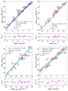 |
Fig. 1. Observed correlations for our galaxy sample. Upper left panel: L1.4 GHz as a function of the SFR. The blue solid line is the best fit to the data, and the shaded region its 68% confidence level. For comparison, the yellow dashed and green dotted lines show the Yun et al. (2001) and Bell (2003) relations, respectively. Upper right panel: L1.4 GHz as a function of LIR. The grey solid line is the best fit to the data, and the shaded region its 68% confidence level. For comparison, the green dotted line shows the Bell (2003) relation. Lower left panel: Lγ as a function of L1.4 GHz. The cyan solid line shows the best fit to the data, and the shaded region its 68% confidence level. For comparison, the brown dashed line shows the Ackermann et al. (2012) relation. Lower right panel: L150 MHz as a function of the SFR. The green solid line is the best fit to the data, and the shaded region its 68% confidence level. For comparison, the red dotted and violet dashed lines show the Gürkan et al. (2018) and Wang et al. (2019) relations, respectively. In all cases, the corresponding residuals weighted by their standard deviation are shown in the bottom panel; the black dotted lines correspond to 3σ. |
This analysis shows that the luminosities we calculate for the restricted sample of galaxies detected in γ rays are consistent with those obtained by other authors, and that they follow the global trend found for more general samples of SFGs observed in radio. This supports that the global radio emission of these galaxies does not present any particular characteristic with respect to that shown by more general samples of galaxies.
As a by-product, a fit of a power law to the relation between γ-ray and radio luminosities (Lγ = A(L1.4 GHz/1021 W Hz−1)m) gives m = 1.26 ± 0.10, log A = 39.04 ± 0.10, and a dispersion of 0.5 dex. This slope is marginally steeper than the value previously reported by Ackermann et al. (2012), who finds a slope of 1.10 ± 0.05. These differences may be due to the size of our sample, which is almost twice as large as that of Ackermann et al. (2012), and also due to the self-consistent and updated values of distances and fluxes we use. We show the resulting correlation in the lower left panel of Fig. 1, together with the Ackermann et al. (2012) relation.
2.3. The L150 MHz–SFR
At low radio frequencies (≲300 MHz) some SFGs show a flattening of their spectra. This may be caused by partial absorption of the synchrotron emission by ionised gas, or by energy losses and propagation effects of CRs (Marvil et al. 2015; Chyży et al. 2018). Therefore, low-frequency data can be useful to infer the absorbing mechanisms and properties of the medium.
Eleven galaxies in our sample (M 31, NGC 253, SMC, M 33, LMC, NGC 2146, NGC 2403, M 82, NGC 3424, Arp 299, Arp 220) have fluxes at 150 MHz available in the literature. For NGC 1068 we take the flux at 145 MHz and the spectral index given by Kuehr et al. (1981), and extrapolate the flux to 150 MHz. In all cases we derive the corresponding luminosities at this frequency (L150 MHz) using the K20 distances. We report these values in Table 1, together with the respective references. In the cases of M 31 and Arp 299 we assumed a typical flux error of 10%.
A power-law fit to the data,  , yields a value of m = 0.98 ± 0.13 and log A = 21.7 ± 0.15, with a dispersion of 0.5 dex. In the lower right panel of Fig. 1 we show the derived L150MHz–SFR correlation, together with those estimated by Wang et al. (2019) and Gürkan et al. (2018). Different works studied this correlation using much larger samples (Calistro Rivera et al. 2017; Read et al. 2018; Smith et al. 2021), reporting values between m = 1.07 (Gürkan et al. 2018) and 1.37 (Wang et al. 2019). Our slope is compatible with that of Gürkan et al. (2018), but our data points fall systematically below the fit of these authors. Given the precision of radio data, this points to a systematic difference in the SFRs whose origin may be the different estimators used (UV–IR proxies in our case, multiwavelength photometric fits in theirs). These authors state that the SFRs provided by their method differ by ∼0.2 dex from those obtained from Hα luminosities, which are in general agreement with ours (see K20). A correction of 0.2 dex in SFR to their fit would bring it into agreement with our data, strongly suggesting that the difference in SFR estimation methods is responsible for this systematic departure. Regarding Wang et al. (2019), the value that they report is derived from a sample using only galaxies above their completeness limit (Ṁ∗ ≈ 3 M⊙ yr−1). Their best fit using all the data, which has better statistics due to the larger number of galaxies at low SFRs, has a lower slope of m ≈ 1.1 in better agreement with ours. Although the 150 MHz data are not homogeneous because the fluxes were obtained from different surveys, and with different criteria for the flux density integration, they deserve to be studied because they provide unique constraints on the properties of non-thermal emission of SFGs. We keep this caveat in mind when interpreting results based on these data.
3. The model
We developed a non-thermal emission model to understand the observed L1.4 GHz–SFR correlation (Sect. 2.2), while also contemplating the Lγ–SFR (Sect. 2.1) and L150 MHz–SFR (Sect. 2.3) relations. The fact that two integrated properties of galaxies are involved in these correlations (the integrated non-thermal luminosity and the SFR) makes it reasonable to describe their emission based on the global CR energy balance. It is sensible to address the comprehension of the correlations between the non-thermal luminosity and the SFR in terms of a population of non-thermal particles that is injected at a rate that depends on the SFR of the galaxy. We further assume that the galactic environment in which these particles are injected is homogeneous and stationary. We self-consistently calculate the energy losses, diffusion, and advection of these relativistic particles and their non-thermal radiative output, corrected by the relevant absorption effects. In what follows we detail how we incorporate all this physics in a model that is valid over a broad range of SFRs.
3.1. CR injection and transport
We model the galaxy emission region as a disc of radius R and height 2H with constant gas density, and in which acceleration sites are uniformly distributed. We adopt R = 1 kpc and H = 0.2 R suggested by K20. Following the standard prescriptions of diffusive shock acceleration at SNRs (e.g. Axford et al. 1977; Bell 1978; Blandford & Ostriker 1978), we assume that CRs are steadily injected in the system according to
![Mathematical equation: $$ \begin{aligned} Q_i(E) = Q_{0,i} E^{-\alpha } \exp {\left[-(E/E_{\mathrm{max}, i})^{\zeta _i}\right]}, \end{aligned} $$](/articles/aa/full_html/2022/01/aa41295-21/aa41295-21-eq5.gif) (1)
(1)
where i = e, p (electrons and protons), α = 2.2 is the spectral index (Lacki & Thompson 2013), Emax is the maximum particle energy (assumed to be 1015 eV), and ζp, e = (1, 2) (Zirakashvili & Aharonian 2007; Blasi 2010). The normalisation constant Q0, i is computed as
 (2)
(2)
assuming that the supernova rate of the galaxy is ℛSN = (83 M⊙)−1 Ṁ∗, consistent with the Chabrier (2003) initial mass function (IMF), and that a fraction ξCR = 10% of the supernova energy (ESN = 1051 erg) is converted in CRs. We adopt Emin, p = 1.2 GeV as the minimum proton energy. Moreover, this energy is distributed as Q0, p/Q0, e = 50; this proton-to-electron ratio is supported by multiwavelength modelling and observations (Torres 2004; Merten et al. 2017; Peretti et al. 2019; Yoast-Hull et al. 2013). We note that a slightly different value compared to our benchmark assumption (within a factor of two) only affects the emission from primary electrons (also within a factor of two), which does not significantly impact our global results.
Young massive star clusters, as discussed in Morlino et al. (2021) can be additional acceleration sites for CRs where diffusive shock acceleration is inferred to be efficient possibly up to PeV levels. Even though these sources can play an important role as acceleration sites, it is not clear yet to what extent they can contribute to the bulk of galactic CRs where, to date, SNRs are believed to be dominant. Therefore, we work under the assumption that SNRs are dominating the injection of the bulk of CRs. Nevertheless, a second population of galactic accelerators (e.g. young massive star clusters) is unlikely to change our main results because the acceleration efficiency values of the two components are adjusted to produce a total CR power similar to that used here.
Electrons and protons experience different losses, which can be divided into radiative, non-radiative, and escape. Electrons suffer radiative losses via synchrotron radiation, inverse Compton (IC) up-scattering of IR photons, and relativistic Bremsstrahlung (BS). Protons lose energy via inelastic p − p collisions. For both particle species the non-radiative losses are due to ionisation. We refer to K20 for the exact expressions used to calculate the corresponding timescales. In particular, for the IC process we adopt the formalism developed by Khangulyan et al. (2014), which accounts for the complete differential cross-section in the Thomson and the Klein–Nishina regimes. Finally, diffusion and advection regulate the particle escape from the emission region. We discuss the details of escape timescales in the following section.
The balance between injection and loss mechanisms leads to the following approximate steady-state solution for the particles distribution in the galaxy
 (3)
(3)
where  and
and ![Mathematical equation: $ \tau_{\mathrm{loss}} = 1/[\tau_{\mathrm{esc}}^{-1} + \tau_{\mathrm{cool}}^{-1}] $](/articles/aa/full_html/2022/01/aa41295-21/aa41295-21-eq9.gif) . Here τesc is the characteristic CR escape time computed as
. Here τesc is the characteristic CR escape time computed as  and
and  , where each τj represents the CR cooling time by each different cooling mechanism.
We note that this equation is almost equivalent to the standard leaky box solution, Ni(E)=Qi(E) τloss(E), with the benefit that it yields a more precise normalisation for injection indices α > 2 when cooling dominates over escape.
3.2. Secondary products
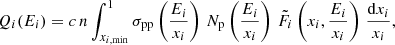
Here we present the formulae used to calculate γ rays and secondary electron spectra produced in p − p interactions. Following Kelner et al. (2006), the emissivity of these secondary products i = γ, e can be summarised in two different formalisms depending on the energy Ei of the resulting particle. In the following equations we denote xi = Ei/Ep.
For Ei > 100 GeV the emissivity formula is
 (4)
(4)
with σpp the cross section for inelastic p − p scattering
![Mathematical equation: $$ \begin{aligned} \sigma _{\rm pp}(E) = \left(34.3 + 1.88 L + 0.25 L^2\right) \times \left[1-\left(\frac{E_{\rm th}}{E}\right)^4\right]^2\,\mathrm{mb}, \end{aligned} $$](/articles/aa/full_html/2022/01/aa41295-21/aa41295-21-eq13.gif) (5)
(5)
where Eth = 1.22 GeV is the threshold energy for π0 production, L = ln(E/TeV), and κ = 0.5 is the process inelasticity;  and
and  are given in Eqs. (58)–(61) and (62)–(65) of Kelner et al. (2006), respectively.
For energies Ei ≤ 100 GeV we describe the emissivity by the δ-functional approximation (Aharonian & Atoyan 2000):
 (6)
(6)
Here n is the number density of the ISM, mp and mπ are respectively the masses of the proton and the pion, Eπ is the pion energy,  , Kπ ≈ 0.17 is the fraction of kinetic energy transferred from the parent proton to the single pion, and
  and
and  are defined in Eqs. (36)–(39) from Kelner et al. (2006) (see also Appendix C).
3.3. Free-free absorption and emission
Part of the ionised gas in SFGs fills uniformly the ISM, whereas another part is concentrated in HII regions randomly distributed over the disc. This gas emits free-free radiation in the radio band. To estimate this emission, we consider that the ionised gas is homogeneously distributed in the same volume as the CRs. In addition, this gas can be optically thick to the low-frequency (thermal and non-thermal) radio emission. Our model has two free parameters that determine the impact of the free-free absorption and emission processes: the electron temperature Te and the ionisation fraction ρ, defined here as the ratio of ionised to total number densities. Thus, we compute the absorbed free-free thermal luminosity at a frequency ν, Lff(ν), following the Olnon (1975) formalism for a homogeneous cylinder seen face-on, valid in the Rayleigh-Jeans regime (hν ≪ kTe, where h and k are the Planck and Boltzmann constants, respectively)
 (7)
(7)
where τff = αff(ν) l is the optical depth, l = 2H is the length of the ionised region along the line of sight, and αff is the absorption coefficient for photons of frequency ν. This coefficient is given by Rybicki & Lightman (1986)
![Mathematical equation: $$ \begin{aligned} \alpha _{\mathrm{ff}} = 3.7 \times 10^8 \rho ^2 n^2 T_{\rm e}^{-1/2} Z^2 \nu ^{-3} \left[1-\exp {\left(-\frac{h\nu }{kT_{\rm e}}\right)} \right]\bar{g}_{\rm ff}, \end{aligned} $$](/articles/aa/full_html/2022/01/aa41295-21/aa41295-21-eq21.gif) (8)
(8)
where Te the ionised gas temperature and  is the mean Gaunt factor (e.g. Leitherer et al. 1995)
 (9)
(9)
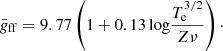
Following Tielens (2005), we assume a constant ionisation fraction ρ = 0.05 throughout the whole SFR range, and we explore the impact of higher values, up to 0.1, on the luminosity–SFR correlations. In SBGs and ULIRGs the ISM conditions are less well-known. Despite the high star formation activity and supernova rate, most of the ionised components may be removed from the central galactic region and load galactic winds. This would lead to extremely low values of the ionisation ratio down to 10−4 (Krumholz et al. 2020). We take this into account by exploring scenarios where ρ is assumed to have such a low value.
The warm neutral and ionised medium phases of the ISM are inferred to have an average temperature of 104 K. However, depending on the fraction of cooler neutral or hot ionised components, the effective ISM temperature could possibly differ by about one order of magnitude (Quireza et al. 2006). Therefore, we assume Te = 104 K as a reference value and explore the impact of an order of magnitude change in its value.
In a similar manner, we obtain the outgoing non-thermal flux of the whole emission region by solving the corresponding radiative transport equation (see Rybicki & Lightman 1986). Modelling the emission region as a homogeneous face-on cylinder, the absorption-corrected synchrotron luminosity is
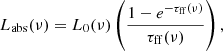 (10)
(10)
where L0 is the unabsorbed luminosity produced by non-thermal radiative processes in our model.
4. Modelling and scale relations
The SFR is the only independent variable in our model. We assume that the energy injected into protons and electrons depends linearly on the SFR (Eq. (2)). The observed correlations presented in Sect. 2 differ from linearity, which suggests that there is also a dependence of the main galactic properties on the SFR. In this section we are interested in finding simple parametrisations for the density n, the IR radiation field, and the magnetic and velocity fields with the SFR, motivated by physical and observational arguments.
4.1. Densities and LIR
We link the IR luminosity to the SFR by using the relation of Bell (2003), adapted to a Chabrier (2003) IMF
![Mathematical equation: $$ \begin{aligned} \dot{M}_{*}[M_\odot \,\mathrm{yr}^{-1}] = 1.72 \times 10^{-10} \frac{L_{\rm IR}}{L_\odot } \left(1 + \sqrt{\frac{10^{9}}{L_{\rm IR}/L_\odot }}\right)\epsilon , \end{aligned} $$](/articles/aa/full_html/2022/01/aa41295-21/aa41295-21-eq25.gif) (11)
(11)
with ϵ = 0.79 (Crain et al. 2010) and LIR the total infrared luminosity between 8 and 1000 μm. For the calculation of the IC interactions we introduce a dilution factor of the energy density of the IR radiation field with respect to the one corresponding to a black body. For a disc geometry this factor is Σ = LIR/(8πR2σSBT4), where σSB is the Stephan-Boltzmann constant.
Finally, the scaling of the density n with the SFR can be set by using the Kennicutt-Schmidt (K-S) law (Kennicutt 1998; Kennicutt & Evans 2012; de los Reyes & Kennicutt 2019). This law gives the correlation between the surface densities of SFR (ΣSFR) and cold gas mass (Σgas) of galaxies. Assuming that the emitter is a cylinder of radius R and thickness 2H (K20), we get
 (12)
(12)
4.2. Magnetic field
Robishaw et al. (2008) showed that strong magnetic fields (B of the order of milligauss, mG, hundreds of times stronger than in our Galaxy) pervade the ISM of high SFR objects, such as ULIRGs, suggesting a strong dependence of B on the level of source activity. Therefore, a detailed modelling of the transport of CR-electrons and their associated non-thermal radio emission requires a careful treatment of the magnetic field and its dependence on the SFR. For this reason, we improved the model developed in K20 proposing the following scaling
 (13)
(13)
where the normalisation factor B0 is a free parameter and for the index β we explore three possible scenarios, β = 0.3, 0.5, 0.7, based on the equipartition arguments described below.
The weakest scaling is obtained relying on a stationary condition of magnetohydrodynamic (MHD) turbulence in the ISM plasma. The MHD turbulence reaches its stationary state when the magnetic field growth produced by turbulence-induced field line stretching is balanced by the back-reaction of the magnetic field itself (Groves et al. 2003). Such a condition results in equipartition between the energy density of the magnetic field and the kinetic energy density of the gas. This yields a scaling  , which is in good agreement with numerical simulations that report exponent values in the range 0.4−0.6 (Groves et al. 2003). By applying the K-S scaling (
 ) one can retrieve the index β ≈ 0.3. The second scenario is based on an equipartition condition between magnetic field and starlight, namely UB ≈ Urad. This condition, often quoted in the literature (e.g. Murphy 2009; Lacki et al. 2010; Yoast-Hull et al. 2016), is motivated by the assumption that the radiation pressure drives the turbulence in the ISM, which in turn determines the strength of the magnetic field. The linear relation between the SFR and the starlight results in the scaling β ≈ 0.5. The third scenario considered relies on the stability of the galactic disc. As discussed by Lacki et al. (2010) (see also Parker 1966), the equipartition between the gas pressure at the mid-plane of the disc (
 ) and the magnetic field pressure (B2/8π) provides a natural limit for the magnetic field strength; higher values would make the galactic disc unstable. This condition, once the Kennicutt scaling is applied, leads to β = 0.7.
We assumed β = 0.3 as the fiducial value for the magnetic field index. In addition, we explored other prescriptions with a stronger B scaling (β = 0.5, 0.7), which could be consistent with a more relevant molecular phase of the ISM in environments with high SFR. We adopted B0 = 100 μG as a fiducial normalisation, which yields B-values in agreement with the expected values for normal starbursts galaxies (see also Peretti et al. 2019) and with that inferred for the Galactic central region (see Ferrière 2009; Lacki & Thompson 2013). We also explored different values of B0 across an order of magnitude to cover the different inferred values for the average magnetic field in SFGs, ranging from ∼μG in low SFR galaxies (Ferrière 2010; Jurusik et al. 2014) to ∼mG for ULIRGs (Robishaw et al. 2008).
4.3. Advection
Winds are ubiquitous in SFGs and are possibly one of the most spectacular consequences of their star formation activity. They are capable of driving mass out of galaxies at a rate of several M⊙ yr−1 with velocities up to 103 km s−1 (see Veilleux et al. 2005). The mechanism(s) powering galactic winds are likely to depend on the SFR. In SBGs they arise from the combined effect of mechanical energy and heating produced by supernovae, and radiation pressure from young stars (Zhang 2018). On the other hand, these effects are unlikely to be mainly responsible for wind launching in galaxies with mild SFRs; instead, the CR pressure seems to play the key role. In particular, the gradient of escaping CRs can be strong enough to overcome the gravitational pull and lift the ISM into the halo (Breitschwerdt et al. 1991; Recchia et al. 2016). In addition, in the case of SBGs, CRs cool more efficiently via p − p collisions and their contribution to powering galactic winds could be minor, but this is still under debate given the importance of the CR pressure exerted on the cold interstellar gas (Bustard & Zweibel 2021).
The effect of galactic winds on the transport of CRs needs to be taken into account. We thus consider that particles are advected away from the galaxy with an energy-independent characteristic time
 (14)
(14)
where vadv is the SFR-dependent advection speed.
We divide the whole galaxy population into two classes: high SFR objects and mild SFR objects. We assume that objects with a star formation higher than the MW, Ṁ∗ ≳ 2 M⊙ yr−1, are characterised by a starburst-driven wind, vsw = 400 km s−1 (see also K20, Yoast-Hull et al. 2013; Peretti et al. 2019). For objects with Ṁ∗ < 2 M⊙ yr−1, we assume that the galactic wind is CR-driven. In this scenario, Recchia et al. (2016) have shown that, at the base of the wind, the dominant advection velocity is the Alfvén speed. Therefore, we consider that particles are advected away from the galactic box at the local Alfvén speed,  . Putting all this together, we define the combined advection velocity over the entire SFR range as
 (15)
(15)
and we assume vadv = vb(Ṁ) to compute the Eq. (14). In addition, we explore alternative scenarios in which the nature of the advection speed is unique (either vA or vsw) for the entire SFR range considered.
4.4. Diffusion
Diffusion is a fundamental aspect of CR physics. At the microscopic level this phenomenon consists of resonant pitch-angle scattering of CRs with the local average magnetic field, taking place when the Larmor radius approaches the wavelength of local magnetic field disturbances (e.g. Alfvén waves, as discussed in Blasi 2013). At the macroscopic level, this small-scale interaction results in a diffusive motion of CRs, where the confinement properties of the system are parametrised by the diffusion coefficient, D. This coefficient holds all information that effectively characterises diffusion, such as the turbulence properties of the medium.
We compute the diffusion coefficient adopting the quasi-linear theory formalism
 (16)
(16)
where v(E) is the particle speed, rL is the Larmor radius, lc represents the coherence length of the magnetic field, and δ characterises the nature of the turbulence. In particular, we have δ = 1/3 for the Kolmogorov turbulence, and δ = 1, 0.5 for Bohm and Kraichnan turbulence. In this work we assume Kolmogorov turbulence, δ = 1/3, as our benchmark case, in agreement with current observations of the boron-to-carbon ratio in the Galaxy (Aguilar et al. 2016). We assume that supernovae are responsible for the injection of the turbulence in the system. Therefore, we compute  as the average separation between SNRs in the galactic box, where we adopt a typical value for the SNR lifetime τSNR = 3 × 10⁴ yr (Truelove & McKee 1999). We also impose that such a parameter cannot be smaller than the typical dimension of a middle-aged SNR, namely lc ≳ 10 pc.
The diffusion coefficient defined in Eq. (16) is assumed to be homogeneous in the whole galactic box. This allows us to define the characteristic timescale, τD, in which particles diffuse away from the galaxy
 (17)
(17)
We give the explicit dependency of τD on the SFR in Appendix B.
5. Results and discussion
To investigate how star formation influences the transport of CRs in SFGs, we set up a benchmark parameter configuration (scenario (0) in Table 2), to compute the global properties of galaxies throughout the whole SFR range (10−2 − 103 M⊙ yr−1), according to the scaling relations discussed in Sect. 4. We compare the timescales of the different processes involved, and solve the transport equation (Eq. (3)) following the prescriptions of Sects. 3 and 4, to determine the main characteristics of CR transport in different ranges of SFR. We present the results for this scenario in Sect. 5.1.
Values of the free parameters of our model (index of B(∗) relation, its normalisation, ionised gas fraction, temperature of the ionised gas) for all the scenarios considered.
The transport of CRs shapes the non-thermal SED, and in turn each luminosity–SFR relation. We focus especially on the impact of different CR transport conditions on these relations. We therefore explore the outcome of our model in terms of the photon SED, from which we extract the integrated luminosity in the Fermi-LAT energy band (0.1−100 GeV) and the monochromatic luminosities at 1.4 GHz and 150 MHz.
We define an upper bound to the luminosity as a function of the SFR (calorimetric limit) in our model, to assess the ability of SFGs to cool CRs, converting their energy into radiation. This limit is built under the following conditions: (i) the escape is artificially turned off so that all injected particles cool inside the source; (ii) the non-thermal emission is not absorbed. This leads to maximum values  ,
,  , and
, and  for each SFR.
We finally analyse the robustness of the model by exploring its parameter space, in order to assess the impact of different assumptions on the luminosity–SFR correlations. The scenarios considered are listed in Table 2. Each scenario from (1) to (8) represents a single parameter variation with respect to the benchmark scenario. We present, discuss, and compare our results for the three luminosity–SFR correlations in Sects. 5.2, 5.3, and 5.5.
5.1. Transport properties of the benchmark scenario
The transport of electrons and protons in SFGs is strongly influenced by the average properties of the ISM, and in turn by their SFR. In this section we present the main transport properties of the benchmark scenario throughout the SFR range, analysing separately electrons and protons. In order to highlight the evolution of the transport condition with the SFR, we show in the upper (lower) panels of Fig. 2 the timescales of the relevant processes for electrons (protons) at two different values of the SFR: 0.1 M⊙ yr−1 and 10 M⊙ yr−1.
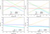 |
Fig. 2. Cooling and escape times for primary electrons (upper panels) and protons (bottom panels) as a function of energy in scenario (0). Left panels: typical case of a low SFR galaxy (Ṁ∗ = 0.1 M⊙ yr−1). Right panels: typical case of a high SFR system (Ṁ∗ = 10 M⊙ yr−1). Solid lines represent different cooling processes: synchrotron (pink), ionisation (yellow), Bremsstrahlung (red), IC (green), and p − p (blue). The black dashed lines are for diffusion, whereas the grey double-dot-dashed lines are for advection. |
Electrons. Ionisation losses dominate the transport of electrons with Ee < 0.1 GeV throughout the whole SFR range, while at higher electron energies the dominant loss mechanism depends on the SFR.
In the low SFR range, Ṁ∗ ≲ 1 M⊙ yr−1, electrons with energies between 0.5 GeV and 10 GeV escape efficiently from galaxies, whereas synchrotron confines electrons at higher energies. As the SFR increases, Bremsstrahlung losses compete with the escape at Ee ∼ 1 GeV, while synchrotron keeps dominating the high energy domain together with IC scattering. In particular, the latter increases its relative importance for increasing SFR and eventually becomes the dominant cooling mechanism for SFR ≳ 102 M⊙ yr−1. Electron calorimetry is achieved for Ṁ∗ ≳ 5 M⊙ yr−1, at which Bremsstrahlung dominates the cooling of GeV electrons; higher energy electrons are cooling-dominated for all SFR ranges.
Protons. The transport of protons is regulated by the competition between escape (diffusion and advection) and energy losses (p − p collisions). At low SFRs, Ṁ∗ ≲ 1 M⊙ yr−1, most of the protons escape via diffusion for Ep ≳ 10 GeV and via advection at lower energies. At higher SFRs, up to a few tens of M⊙ yr−1, p − p losses become the dominant loss mechanism. However calorimetry is not completely achieved because the advection and p − p timescales remain comparable. A transition to a diffusive-dominated transport also occurs in the multi-TeV range. Finally, we note that galaxies behave like good proton calorimeters for SFRs ≳ 30 M⊙ yr−1.
5.2. The Lγ–SFR relation
We define Lγ as the integrated luminosity in the 0.1−100 GeV energy band, and we show in Fig. 3 the Lγ–SFR relation obtained for the benchmark scenario. The main contribution to Lγ comes from the p − p interaction, while γ rays of leptonic origin are subdominant (see Fig. B.1). In agreement with K20, the shape of the Lγ–SFR relation at low SFRs is influenced by the escape of most of the injected protons, whereas at high SFRs sources approach the calorimetric limit, where the correlation becomes a linear scaling. We also show the results obtained assuming a unique nature of the advection speed throughout the whole SFR range, namely vadv = vA or vadv = vsw. Since vsw > vA (vA ≳ 50 km s−1 for the fiducial scenario), the CR escape is more efficient when vadv = vsw and consequently the γ-ray luminosity is reduced. Our benchmark case is in good agreement with the best fit of the observed sample.
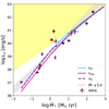 |
Fig. 3. Lγ–SFR relation for scenario (0) using three different prescriptions for vadv: va (solid blue line), vsw (solid pink line), and vb from Eq. (15) (violet dashed line). The grey line and shaded band indicate the best fit to the data (purple circles) and its 1σ confidence region, respectively. The yellow region is forbidden by the calorimetric limit. |
Variations of β, B0, and Te do not affect the emission of protons and, consequently, the Lγ–SFR correlation is not altered. On the contrary, the variation of the ionisation fraction ρ (scenarios (5) and (6)) modifies the CR escape through vA at low SFRs, affecting the total source luminosity.
As described in Sect. 3.3, we explore values for the ionisation fraction down to 10−4. While these values can characterise powerful starbursts such as ULIRGs, they are unlikely to be physical in standard SFGs with low SFRs. Such a small ionisation fraction leads to an Alfvén speed larger than the average velocity of starburst superwinds resulting in an advection dominated transport at odds with observations of CRs (Blasi 2013) and γ rays (Ajello et al. 2020). The scenario ρ = 0.1 does not show any relevant modifications with respect to the benchmark scenario since the dominant escape mechanism is diffusion.
As mentioned in Sect. 4, we improved the model of K20 introducing a SFR-dependent diffusion coefficient and a two-fold nature of the wind, while neither diffusion coefficient nor the wind velocity depend on the SFR in K20. Despite these differences, the results presented here are compatible with the benchmark scenario discussed in K20.
The Lγ–SFR relation obtained here is in good agreement with the trend of data, and consistent with the results presented in K20. The model approaches the calorimetric limit (limit of the yellow shaded region) for Ṁ∗ ≥ 30 M⊙ yr−1, above which galaxies show a calorimetric behaviour. NGC 3424 and 4945 luminosities are incompatible with this limit by 4.1 and 6.4 times their errors. As discussed in K20, the former probably harbours a low-luminosity AGN, whereas the SFR of the latter may have been underestimated due to its obscuration and inclination to the line of sight.
5.3. The L1.4 GHz–SFR relation
The emission at 1.4 GHz is set by three processes: synchrotron radiation from both primary and secondary electrons, free-free (thermal) emission of the ionised gas, and free-free absorption produced by this same gas. Synchrotron radiation dominates the L1.4 GHz throughout the entire SFR range, as shown in Fig. 4 (left panel), while free-free emission and absorption become relevant only at high SFR. The thermal contribution eventually becomes comparable to that of synchrotron at Ṁ∗ > 100 M⊙ yr−1 (see Fig. B.1).
 |
Fig. 4. Results for scenario (0) using vadv = vb from Eq. (15) (violet dashed line). Left panel: L1.4 GHz–SFR relation. The green dashed and dot-dashed lines represent the primary and secondary synchrotron electron contribution, respectively, and the dotted violet line the free-free contribution. The total emission at L1.4 GHz is also shown for two different prescriptions for vadv, vA (solid blue line) and vsw (solid pink line). Right panel: Lγ–L1.4 GHz relation. In both panels the grey shaded band indicates the 1σ confidence region of each fit (solid grey line) to the data sample (purple points). |
The emission of primary electrons dominates the L1.4 GHz–SFR correlation in the low SFR range (≲1 M⊙ yr−1), whereas synchrotron from secondaries gradually increases with the SFR and overcomes that of primaries at high SFRs (see respectively green dot-dashed and dashed lines in left panel of Fig. 4). This behaviour is a direct consequence of the transport condition of the parent protons. In particular, the higher the SFR, the higher the gas density and thus the rate of interaction of protons.
The secondary-to-primary ratio increases with the SFR as a consequence of the increasing level of calorimetry up to ≳30 M⊙ yr−1, where full calorimetry is achieved and the secondary-to-primary ratio becomes constant. This result is found to be in agreement with those of Peretti et al. (2019).
In SFGs with SFRs ≲ 102 M⊙ yr−1, L1.4 GHz is dominated by the synchrotron emission, hereafter  . In order to understand the shape of the correlation, we note that
  is dominated by the emission of ∼GeV electrons, independently of the SFR. This electron-energy band is characterised by the competition of several cooling and escape mechanisms, so that the slope of the particle energy distribution can range from α − 1 when ionisation dominates to α + 1 when synchrotron dominates. In addition, secondary electron emission depends on the SFR through both the density of the medium and the parent proton transport (see Sect. 3.2). This leads to a complex dependence of
  on the SFR, which we parametrise as
 (18)
(18)
where η is the slope of the synchrotron luminosity in the logarithmic L1.4 GHz–SFR correlation. We note that this component dominates the L1.4 GHz–SFR correlation up to ∼102 M⊙ yr−1 for the benchmark scenario, where we constrain η to the range 0.8−1.8. In particular, the slope of the correlation is steeper in the low SFR range, where the relative contribution of secondaries increases with the SFR. At high SFRs, the transport of protons also becomes calorimetric and the slope of the correlation softens (see Appendix B for a detailed discussion). We note that in calorimetric conditions η < 1. This results from the higher efficiency of ionisation and Bremsstrahlung in cooling GeV electrons.
The relevance of thermal processes increases for higher SFRs as a consequence of the higher density of the ISM and our assumption of constant ionisation fraction ρ throughout the whole SFR range. In particular, the thermal contribution to L1.4 GHz is at the level of ∼5% for low SFR galaxies; this is consistent with values reported by Condon (1992) for the thermal emission in the MW and M 82. At high SFRs (≳100 M⊙ yr−1) the thermal contribution is ∼50%, and the free-free absorption also becomes significant. Nonetheless, assumptions in the ionisation fraction ρ impact on the relative importance of the free-free processes, as we discuss below.
Finally, we compare our benchmark model with the data presented in Table 1. We highlight that the coexistence of both primary and secondary synchrotron electron components is necessary to reproduce the slope of the L1.4 GHz–SFR correlation. In the right panel of Fig. 4 we present observational data in the Lγ–L1.4 GHz plane and compare them with the outcomes of our model; we obtain a good agreement throughout the whole SFR range.
5.4. Parameter dependence of the L1.4 GHz–SFR relation
In this section we discuss the impact of parameter variations on the L1.4 GHz–SFR correlation.
Magnetic field index. As the thermal emission is unaltered by changes in β, here we focus only on the synchrotron component. The top panels in Fig. 5 illustrate how the variation of β (scenarios (1) and (2)) affects the slope of the L1.4 GHz–SFR and L1.4 GHz–LIR correlations.
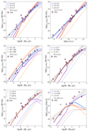 |
Fig. 5. Model relations for the different scenarios considered (Table 2). The grey shaded band indicates the 1σ confidence region of each fit (grey solid line) to the data sample (purple points). In all panels the dotted lines represent the thermal emission, the dashed lines the non-thermal emission, and the solid line the total emission. Upper panel: for scenarios (0), (1), and (2) the L1.4 GHz–SFR relation (left) and the L1.4 GHz–LIR relation (right) are shown. Middle panel: for scenarios (0), (3), and (4) (left) and (0), (5), and (6) (right) the L1.4 GHz–SFR relation is shown. Bottom panel: for scenarios (0), (7), and (8) the L1.4 GHz–SFR relation (left) is shown and for scenarios (0), (5), and (6) the L150 MHz–SFR relation (right) is shown. |
In particular, the larger the value of β, the steeper the slope η of the L1.4 GHz–SFR correlation. This is a natural consequence of the dependence of the synchrotron luminosity on the magnetic field which, for larger β, presents a larger variation throughout the SFR range (see Appendix B).
At the same time, lower values of B resulting from β > 0.3 at low SFRs reduce the escape time, which in turn reduces the luminosity and makes the correlation steeper. The benchmark scenario with β = 0.3 provides the best fit to the general trend of the observed data. However, the assumption β = 0.5, in agreement with Lacki et al. (2010), is slightly more appropriate while fitting data at high SFR. The scenario assuming β = 0.7 is disfavoured when compared with data in the entire SFR range, whereas, as in the case of β = 0.5, it can be adopted to describe the high SFR range.
Magnetic field normalisation. A variation of B0 (scenarios (3) and (4)) results in a different normalisation of the correlation curve of about a factor ∼1.5 − 4. We show these results in the middle left panel of Fig. 5. This behaviour is in agreement with the dependence of the synchrotron luminosity of a non-thermal electron population with the magnetic field (see e.g. Ghisellini 2013). However, the synchrotron radiation at 1.4 GHz is mostly produced by electrons in the ∼GeV range. At these energies several physical processes compete in shaping the electron energy distribution. This leads to an energy distribution different from a simple power law. Thus, in the context of SFGs, the dependence of L1.4 GHz on the magnetic field strength is not trivial, and a change in the normalisation constant B0 introduces an overall shift which slightly depends on the SFR. Despite this complexity, we show that the parameter B0 does not affect the global slope of the correlation, but only influences its normalisation (see Appendix B for a more detailed and quantitative discussion). The value B0 = 100 is the one that best fits the data. The resulting correlations for B0 = 50 and 500 limit the data above and below, respectively, excluding only NGC 4945.
Ionisation fraction. The impact of different assumptions for the ionisation fraction ρ on the L1.4 GHz–SFR correlation is threefold since it affects: (1) the free-free emission, (2) the free-free absorption, and (3) the advection timescale in low SFGs. The middle right panel of Fig. 5 illustrates the results obtained in the benchmark case (blue lines) compared with ρ = 10−4 (violet lines) and ρ = 10−1 (orange lines).
Although a value of ρ = 0.1 produces results consistent with the observed trend, at high SFR the thermal emission becomes significant and possibly dominates. This is the opposite of what is expected for galaxies like M 82 where the estimated thermal fraction is even lower (∼2%, Basu et al. 2012) than for normal galaxies. The scenario where ρ = 0.1 is therefore unlikely to be realised in nature and at odds with multiwavelength modelling of ULIRGs (see e.g. Yoast-Hull et al. 2017). On the other hand, lower values of ρ reduce the absorption and the relative importance of thermal emission at high SFR. This yields a thermal contribution that is too low with respect to what is generally accepted to hold for normal galaxies (Condon 1992). Finally, ρ = 10−4 underestimates the data at low SFRs, and the model behaviour is similar to that of γ rays.
We conclude that the scenario where ρ = 0.05 is the one that better accommodates the observed data and remains consistent with synchrotron dominating the emission at 1.4 GHz. Although it is tempting to speculate on a possible SFR dependence of ρ, this would introduce further complexity in the model, and we therefore leave it for upcoming investigations.
Electron temperature. Te ∼ 104 K is the standard temperature assumed for the warm ionised ISM. In starburst regions, this gas coexists with a hot and pressurised component resulting from the collective effect of supernovae and stellar winds. This implies that Te > 104 K might be consistent with the average temperature in these environments (Westmoquette et al. 2009). The variation of Te (scenarios (7) and (8)) affects the thermal emission and absorption. This behaviour is shown in Fig. 5 (bottom left panel) from which it can be concluded that values between Te = 104 and 105 K reproduce well the observations, whereas lower values of Te lead to an excessive absorption at high SFR compared to the data trend.
These results can be understood by looking at the physical dependence of the opacity on the temperature. In particular, at a given photon frequency,  , and so the optically thick regime is reached at higher SFRs for higher values of Te. Thus, the absorption of synchrotron radiation decreases with Te.
Finally, we observe that the different assumptions about the temperature do not strongly impact the relative contribution of thermal emission to the L1.4 GHz across the whole SFR range.
5.5. The L150 MHz–SFR relation
The physical processes governing the emission at 150 MHz are the same as at 1.4 GHz (Sect. 5.3). However, at this frequency free-free absorption plays a crucial role. The turnover frequency where τff > 1 increases up to 150 MHz for Ṁ∗ ∼ 10 M⊙ yr−1. Therefore, the 150 MHz synchrotron emission is completely absorbed at high SFRs in our benchmark scenario. This is reflected in the L150 MHz–SFR correlation shown in Fig. 6. This scenario departs considerably from the observed trend of data at high SFRs and cannot reproduce the emission of the ULIRGs. Such a strong absorption is the result of the ionisation fraction assumed, ρ ∼ 5%. In addition, the calorimetric limit determined for the benchmark scenario also shows that it can hardly match the observed fluxes for SFRs ≳ 102 M⊙ yr−1.
 |
Fig. 6. L150 MHz–SFR relation obtained for scenario (0) using three different prescriptions for vadv: vA (solid cyan line), vsw (solid pink line), and vb from Eq. (15) (violet dashed line). The green dashed and green dot-dashed lines represent the primary and secondary electron contributions, respectively, and the dotted violet line represents the free-free contribution. The grey shaded band indicates the 1σ confidence region of the fit (solid grey line) to the data sample (purple points). |
Although the effects of the variation of parameters in the L150 MHz–SFR correlation are similar to those in the L1.4 GHz–SFR correlation, some details are required to determine if it is possible to match the trend of data with a model prediction under different parametric assumptions.
The assumption β = 0.5, as in the case at 1.4 GHz, increases the slope of both the correlation and the calorimetric limit. Moreover, ionisation losses are dynamically important for electrons emitting synchrotron at 150 MHz. In addition, different assumptions for ρ and Te can also mitigate or enhance the absorption as evidenced in the bottom right panel of Fig. 5. As described above for 1.4 GHz, it is hard to find a unique parameter configuration that can accommodate the entire SFR range without being at odds with observations. In particular, we observe that the introduction of a dependence on the SFR for ρ and/or Te would provide a better fit at a high SFR. Such a lack of emission at low radio frequencies was also reported by Schober et al. (2017) who found a similar result studying the correlation at 200 MHz.
6. Conclusions
We investigated how the transport of CRs, produced by sources related to the star formation, shapes the observed Lγ–SFR, L1.4 GHz–SFR, and L150 MHz–SFR correlations for SFGs detected in γ rays. We presented a flexible emission model for SFGs over a broad range of SFRs and compared the theoretical estimates with the most updated observational data available. The main results from our work are summarised as follows:
-
We provide homogeneous radio continuum fluxes and their errors computed directly from images at 1.4 GHz of Stokes-I available in the NRAO/VLASky continuum Survey catalogue for NGC 253, NGC 1068, NGC 2146, NGC 2403, M 82, Arp 220, Arp 299, and NGC 3424. We also computed for the first time the fluxes and the errors for NGC 4945 and Circinus from the new 1.4 GHz Stokes-I continuum image provided by The ASKAP Continuum Survey.
-
We provide the first self-consistent data set at 150 MHz and 1.4 GHz for all galaxies detected in γ rays. We present updated correlations of Lγ–SFR, L1.4 GHz–SFR, and L150 MHz–SFR for these galaxies.
-
The trend followed by the L1.4 GHz–SFR correlation observed in the subsample of SFGs detected at γ rays agrees very well with that obtained from larger surveys of SFGs (Yun et al. 2001; Bell 2003).
-
We revisited the Lγ–L1.4 GHz correlation and found a steeper slope m = 1.26 ± 0.10 (with
 ) with respect to the value reported by Ackermann et al. (2012).
 -
We obtained a slope of m = 0.98 ± 0.13 for the L150 MHz–SFR correlation (with
 ), which is marginally shallower than results reported by other authors (ranging from 1 to 1.3).
 -
We developed a self-consistent model for CR transport and multiwavelength emission suitable to interpret the luminosity–SFR correlation at different energy ranges over a very broad range of SFRs. This model can reproduce reasonably well the observed Lγ–SFR, L1.4 GHz–SFR, and L1.4 GHz–Lγ correlations.
-
A constant ionisation fraction ρ fails to reproduce the L150 MHz–SFR correlation throughout the whole SFR range. In particular, an ionisation fraction of ∼5% at low SFRs is compatible with observations, whereas at high SFRs a value < 1% is favoured to achieve the emission observed in ULIRGs. Small values of ρ would be in agreement with the results of Valdés et al. (2005) who suggest that a significant fraction of the ionising photons may be absorbed by dust. Moreover, Krumholz et al. (2020) propose that typical ionisation fractions in starbursts should be ∼10−4 since the hot gas would be advected in the wind.
-
A scaling law B = B0(Ṁ∗/10 M⊙ yr−1)β is compatible with the observed data for β = 0.3, which suggests that the magnetic field strength is regulated by stationary MHD turbulence. Higher beta values are also compatible with data limited to the range of high SFR. The normalisation value that best describes the magnetic field at 10 M⊙ yr−1 is of the order of 100 μG.
-
The coexistence of synchrotron components from both primary and secondary electrons is mandatory to reproduce the slope of the L1.4 GHz–SFR correlation. Such a slope reflects the transport conditions of primary protons and could provide indications of a transition to a calorimetric regime.
-
High temperatures of 104 − 105 K for the ionised gas are more suitable to explain the emission of the ULIRGs.
-
Galaxies behave as good proton calorimeters for SFR ≳ 30 M⊙ yr−1. Such a calorimetry can be assessed via observations in γ rays. On the contrary, relativistic electrons, although they reach the calorimetric limit for SFR ≳ 5 M⊙ yr−1, are hard to assess given that their emission is not completely dominant for all SFRs in either the radio or the γ-ray band.
-
Different wind prescriptions depending on the SFR of the galaxy yield a good description of the Lγ–SFR correlation. In particular, an Alfvenic wind is proposed to dominate in low-SFR galaxies, whereas a thermally driven wind would better describe the outflow at high SFRs.
The SMC deserves a more thorough discussion. It is the galaxy at the lower end of the SFR range, separated by far from the next one, and therefore may play an important role in model fitting. Its non-thermal luminosity is almost always underpredicted by our models. It might be argued that this is the result of additional contributions from either unresolved point-like sources or from the halo. However, this seems very improbable, due to the short distance and extended nature of this galaxy. The discrepancy can be mitigated taking into account the uncertainty in the current SFR estimates for the SMC. We used the K20 value (0.027 M⊙ yr−1) obtained from an Hα/IR proxy, sensitive to the SFR in a time interval of ∼10 Myr, whereas it has been found that the SMC has a complex SFR history with recent bursts of up to ten times this value (Harris & Zaritsky 2004). An increase in the SFR of the SMC of 0.5−1 dex almost always results in a better agreement between observations and our L1.4 GHz–SFR and L150 MHz–SFR modelled correlations at low SFRs.
Enlarging the current sample of γ-ray emitting SFGs, and developing reliable techniques capable of distinguishing the emission associated with AGN hosted by some galaxies of the sample is necessary to obtain a more accurate Lγ–SFR correlation. A larger sample of galaxies detected in γ rays would also yield a more accurate Lγ − L1.4 GHz correlation, which is important for two reasons. The first is that it could provide an independent method for the classification of γ-ray galaxies, in addition to the standard method based on the spectral index determination. The second reason is that it could be used to estimate the contribution of SFGs to the γ-ray background by extrapolating the radio luminosity function to high redshift.
A careful study of the L150 MHz–SFR correlation is important to assess the extent to which L150 MHz traces star formation. Furthermore, a more refined L150 MHz–SFR correlation would allow us to discern if the SFGs detected in γ rays follow a distinguishable trend with respect to more general samples. Due to the difficulties in reproducing the emission at these low frequencies, in upcoming studies we will address the effect produced on the modelled correlation by an ionisation fraction diminishing with the SFR, or a highly clumped gas distribution resulting in a porous medium. An alternative scenario can be a non-negligible contribution from particles radiating from a region larger than our galactic box, for instance electrons diffusing or advected in the halo (Heesen et al. 2009), or the presence of an additional source or acceleration region (such as a co-existing AGN) not directly related to the SFR (Gürkan et al. 2018).
The next generation of telescopes with better angular resolution and sensitivity will allow us to unravel the morphology of the diffuse non-thermal emitting region in SFGs, possibly resolving the emission coming from the disc from that originated in the halo or wind (see e.g. Romero et al. 2018; Müller et al. 2020; Peretti et al. 2021). The panchromatic view of the SFR–luminosity correlations in SFGs is a key to assessing the physical processes that govern the non-thermal emission of these sources. In particular, we plan to extend the study of luminosity correlations to the VHE and hard X-ray energy bands. The former can provide a unique identification tool for possible new detections by the upcoming Cherenkov Telescope Array (CTA; Cherenkov Telescope Array Consortium 2019). The latter can provide a new powerful tool for investigating the CR transport properties.
Acknowledgments
P.K. and P.B. acknowledge B. Koribalski for help in providing the ASKAP data. The research activity of E.P. was supported by Villum Fonden (project n. 18994) and by the European Unions Horizon 2020 research and innovation program under the Marie Sklodowska-Curie grant agreement No. 847523 “INTERACTIONS”. P.B. acknowledges support from ANPCyT PICT 0773–2017. L.J.P, P.K. and P.B. acknowledge also support from CONICET grant PIP 2014-0265.
References
- Abdo, A. A., Ackermann, M., Ajello, M., et al. 2010a, ApJS, 188, 405 [NASA ADS] [CrossRef] [Google Scholar]
- Abdo, A. A., Ackermann, M., Ajello, M., et al. 2010b, ApJ, 709, L152 [NASA ADS] [CrossRef] [Google Scholar]
- Abdollahi, S., Acero, F., Ackermann, M., et al. 2020, ApJS, 247, 33 [Google Scholar]
- Acciari, V. A., Aliu, E., Arlen, T., et al. 2009, Nature, 462, 770 [NASA ADS] [CrossRef] [Google Scholar]
- Acero, F., Aharonian, F., Akhperjanian, A. G., et al. 2009, Science, 326, 1080 [NASA ADS] [CrossRef] [Google Scholar]
- Ackermann, M., Ajello, M., Allafort, A., et al. 2012, ApJ, 755, 164 [NASA ADS] [CrossRef] [Google Scholar]
- Aguilar, M., et al. (AMS Collaboration) 2016, Phys. Rev. Lett., 117, 231102 [NASA ADS] [CrossRef] [Google Scholar]
- Aharonian, F. A., & Atoyan, A. M. 2000, A&A, 362, 937 [NASA ADS] [Google Scholar]
- Aharonian, F., Yang, R., & de Oña Wilhelmi, E. 2019, Nat. Astron., 3, 561 [Google Scholar]
- Ajello, M., Mauro, M. D., Paliya, V. S., & Garrappa, S. 2020, ApJ, 894, 88 [NASA ADS] [CrossRef] [Google Scholar]
- Axford, W. I., Leer, E., & Skadron, G. 1977, Int. Cosm. Ray Conf., 11, 132 [Google Scholar]
- Ballet, J., Burnett, T. H., Digel, S. W., & Lott, B. 2020, ArXiv e-prints [arXiv:2005.11208] [Google Scholar]
- Basu, A., Mitra, D., Wadadekar, Y., & Ishwara-Chandra, C. H. 2012, MNRAS, 419, 1136 [NASA ADS] [CrossRef] [Google Scholar]
- Bauer, M., Pietsch, W., Trinchieri, G., et al. 2008, A&A, 489, 1029 [NASA ADS] [CrossRef] [EDP Sciences] [Google Scholar]
- Bell, A. R. 1978, MNRAS, 182, 147 [Google Scholar]
- Bell, E. F. 2003, ApJ, 586, 794 [Google Scholar]
- Blandford, R. D., & Ostriker, J. P. 1978, ApJ, 221, L29 [Google Scholar]
- Blasi, P. 2010, MNRAS, 402, 2807 [Google Scholar]
- Blasi, P. 2013, A&ARv, 21, 70 [Google Scholar]
- Blom, J. J., Paglione, T. A. D., & Carramiñana, A. 1999, ApJ, 516, 744 [NASA ADS] [CrossRef] [Google Scholar]
- Breitschwerdt, D., McKenzie, J. F., & Voelk, H. J. 1991, A&A, 245, 79 [NASA ADS] [Google Scholar]
- Bustard, C., & Zweibel, E. G. 2021, ApJ, 913, 106 [NASA ADS] [CrossRef] [Google Scholar]
- Bustard, C., Zweibel, E. G., & Cotter, C. 2017, ApJ, 835, 72 [NASA ADS] [CrossRef] [Google Scholar]
- Bykov, A. M., & Toptygin, I. N. 2001, Astron. Lett., 27, 625 [NASA ADS] [CrossRef] [Google Scholar]
- Bykov, A. M., Marcowith, A., Amato, E., et al. 2020, Space Sci. Rev., 216, 42 [CrossRef] [Google Scholar]
- Calistro Rivera, G., Williams, W. L., Hardcastle, M. J., et al. 2017, MNRAS, 469, 3468 [Google Scholar]
- Chabrier, G. 2003, PASP, 115, 763 [Google Scholar]
- Cherenkov Telescope Array Consortium (Acharya, B. S., et al.) 2019, Science with the Cherenkov Telescope Array, 364 [Google Scholar]
- Chyży, K. T., Jurusik, W., Piotrowska, J., et al. 2018, A&A, 619, A36 [NASA ADS] [CrossRef] [EDP Sciences] [Google Scholar]
- Clemens, M. S., Scaife, A., Vega, O., & Bressan, A. 2010, MNRAS, 405, 887 [NASA ADS] [Google Scholar]
- Condon, J. J. 1992, ARA&A, 30, 575 [Google Scholar]
- Condon, J. J., Huang, Z. P., Yin, Q. F., & Thuan, T. X. 1991, ApJ, 378, 65 [Google Scholar]
- Condon, J. J., Cotton, W. D., Greisen, E. W., et al. 1998, AJ, 115, 1693 [Google Scholar]
- Cox, M. J., Eales, S. A. E., Alexander, P., & Fitt, A. J. 1988, MNRAS, 235, 1227 [CrossRef] [Google Scholar]
- Crain, R. A., McCarthy, I. G., Frenk, C. S., Theuns, T., & Schaye, J. 2010, MNRAS, 407, 1403 [NASA ADS] [CrossRef] [Google Scholar]
- Cristofari, P., Blasi, P., & Caprioli, D. 2021, A&A, 650, A62 [NASA ADS] [CrossRef] [EDP Sciences] [Google Scholar]
- de Cea del Pozo, E., Torres, D. F., & Rodriguez Marrero, A. Y. 2009, ApJ, 698, 1054 [Google Scholar]
- de los Reyes, M. A. C., & Kennicutt, R. C., Jr. 2019, ApJ, 872, 16 [NASA ADS] [CrossRef] [Google Scholar]
- Dennison, B., Balonek, T. J., Terzian, Y., & Balick, B. 1975, PASP, 87, 83 [NASA ADS] [CrossRef] [Google Scholar]
- Domingo-Santamaría, E., & Torres, D. F. 2005, A&A, 444, 403 [NASA ADS] [CrossRef] [EDP Sciences] [Google Scholar]
- Durdin, J. M., & Terzian, Y. 1972, AJ, 77, 637 [NASA ADS] [CrossRef] [Google Scholar]
- Escobar, G. J., Pellizza, L. J., & Romero, G. E. 2021, A&A, 650, A136 [NASA ADS] [CrossRef] [EDP Sciences] [Google Scholar]
- Ferrière, K. 2009, A&A, 505, 1183 [NASA ADS] [CrossRef] [EDP Sciences] [Google Scholar]
- Ferrière, K. 2010, in The Dynamic Interstellar Medium: A Celebration of the Canadian Galactic Plane Survey, eds. R. Kothes, T. L. Landecker, & A. G. Willis, ASP Conf. Ser., 438, 243 [Google Scholar]
- For, B. Q., Staveley-Smith, L., Hurley-Walker, N., et al. 2018, MNRAS, 480, 2743 [NASA ADS] [CrossRef] [Google Scholar]
- Ghisellini, G. 2013, Radiative Processes in High Energy Astrophysics (Berlin: Springer-Verlag), 873 [Google Scholar]
- Groves, B. A., Cho, J., Dopita, M., & Lazarian, A. 2003, PASA, 20, 252 [NASA ADS] [CrossRef] [Google Scholar]
- Guo, X.-L., Xin, Y.-L., Liao, N.-H., & Fan, Y.-Z. 2019, ApJ, 885, 117 [NASA ADS] [CrossRef] [Google Scholar]
- Gürkan, G., Hardcastle, M. J., Smith, D. J. B., et al. 2018, MNRAS, 475, 3010 [Google Scholar]
- Hales, S. E. G., Mayer, C. J., Warner, P. J., & Baldwin, J. E. 1991, MNRAS, 251, 46 [NASA ADS] [Google Scholar]
- Harris, J., & Zaritsky, D. 2004, AJ, 127, 1531 [NASA ADS] [CrossRef] [Google Scholar]
- Heesen, V., Beck, R., Krause, M., & Dettmar, R. J. 2009, A&A, 494, 563 [CrossRef] [EDP Sciences] [Google Scholar]
- Hughes, A., Staveley-Smith, L., Kim, S., Wolleben, M., & Filipović, M. 2007, MNRAS, 382, 543 [Google Scholar]
- Israel, F. P., Mahoney, M. J., & Howarth, N. 1992, A&A, 261, 47 [NASA ADS] [Google Scholar]
- Jokipii, J. R., & Morfill, G. E. 1985, ApJ, 290, L1 [NASA ADS] [CrossRef] [Google Scholar]
- Jurusik, W., Drzazga, R. T., Jableka, M., et al. 2014, A&A, 567, A134 [NASA ADS] [CrossRef] [EDP Sciences] [Google Scholar]
- Kapińska, A. D., Staveley-Smith, L., Crocker, R., et al. 2017, ApJ, 838, 68 [CrossRef] [Google Scholar]
- Kelner, S. R., Aharonian, F. A., & Bugayov, V. V. 2006, Phys. Rev. D, 74, 034018 [Google Scholar]
- Kennicutt, R. C., Jr. 1998, ApJ, 498, 541 [Google Scholar]
- Kennicutt, R. C., & Evans, N. J. 2012, ARA&A, 50, 531 [NASA ADS] [CrossRef] [Google Scholar]
- Khangulyan, D., Aharonian, F. A., & Kelner, S. R. 2014, ApJ, 783, 100 [Google Scholar]
- Klein, U., Lisenfeld, U., & Verley, S. 2018, A&A, 611, A55 [NASA ADS] [CrossRef] [EDP Sciences] [Google Scholar]
- Kornecki, P., Pellizza, L. J., del Palacio, S., et al. 2020, A&A, 641, A147 [EDP Sciences] [Google Scholar]
- Krumholz, M. R., Crocker, R. M., Xu, S., et al. 2020, MNRAS, 493, 2817 [NASA ADS] [CrossRef] [Google Scholar]
- Kuehr, H., Witzel, A., Pauliny-Toth, I. I. K., & Nauber, U. 1981, A&AS, 45, 367 [NASA ADS] [Google Scholar]
- Lacki, B. C., & Thompson, T. A. 2013, ApJ, 762, 29 [NASA ADS] [CrossRef] [Google Scholar]
- Lacki, B. C., Thompson, T. A., & Quataert, E. 2010, ApJ, 717, 1 [Google Scholar]
- Lacki, B. C., Thompson, T. A., Quataert, E., Loeb, A., & Waxman, E. 2011, ApJ, 734, 107 [NASA ADS] [CrossRef] [Google Scholar]
- Leitherer, C., Chapman, J. M., & Koribalski, B. 1995, ApJ, 450, 289 [NASA ADS] [CrossRef] [Google Scholar]
- Lenain, J. P., Ricci, C., Türler, M., Dorner, D., & Walter, R. 2010, A&A, 524, A72 [NASA ADS] [CrossRef] [EDP Sciences] [Google Scholar]
- Lenc, E., & Tingay, S. J. 2009, AJ, 137, 537 [Google Scholar]
- Lisenfeld, U., & Völk, H. J. 2000, A&A, 354, 423 [NASA ADS] [Google Scholar]
- Loiseau, N., Klein, U., Greybe, A., Wielebinski, R., & Haynes, R. F. 1987, A&A, 178, 62 [NASA ADS] [Google Scholar]
- Mancuso, C., Lapi, A., Prandoni, I., et al. 2017, ApJ, 842, 95 [Google Scholar]
- Martin, P. 2014, A&A, 564, A61 [NASA ADS] [CrossRef] [EDP Sciences] [Google Scholar]
- Marvil, J., Owen, F., & Eilek, J. 2015, AJ, 149, 32 [CrossRef] [Google Scholar]
- McConnell, D., Hale, C. L., Lenc, E., et al. 2020, PASA, 37, e048 [Google Scholar]
- Merten, L., Becker Tjus, J., Eichmann, B., & Dettmar, R.-J. 2017, Astropart. Phys., 90, 75 [NASA ADS] [CrossRef] [Google Scholar]
- Morlino, G., Blasi, P., Peretti, E., & Cristofari, P. 2021, MNRAS, 504, 6096 [NASA ADS] [CrossRef] [Google Scholar]
- Müller, A. L., Romero, G. E., & Roth, M. 2020, MNRAS, 496, 2474 [CrossRef] [Google Scholar]
- Murphy, E. J. 2009, ApJ, 706, 482 [Google Scholar]
- Ohm, S., & Hinton, J. A. 2013, MNRAS, 429, L70 [NASA ADS] [CrossRef] [Google Scholar]
- Olnon, F. M. 1975, A&A, 39, 217 [NASA ADS] [Google Scholar]
- Parker, E. N. 1966, ApJ, 145, 811 [NASA ADS] [CrossRef] [Google Scholar]
- Peretti, E., Blasi, P., Aharonian, F., & Morlino, G. 2019, MNRAS, 487, 168 [NASA ADS] [CrossRef] [Google Scholar]
- Peretti, E., Blasi, P., Aharonian, F., Morlino, G., & Cristofari, P. 2020, MNRAS, 493, 5880 [NASA ADS] [CrossRef] [Google Scholar]
- Peretti, E., Morlino, G., Blasi, P., & Cristofari, P. 2021, MNRAS, submitted [arXiv:2104.10978] [Google Scholar]
- Persic, M., & Rephaeli, Y. 2002, A&A, 382, 843 [NASA ADS] [CrossRef] [EDP Sciences] [Google Scholar]
- Persic, M., & Rephaeli, Y. 2010, MNRAS, 403, 1569 [NASA ADS] [CrossRef] [Google Scholar]
- Persic, M., & Rephaeli, Y. 2014, A&A, 567, A101 [NASA ADS] [CrossRef] [EDP Sciences] [Google Scholar]
- Persic, M., Rephaeli, Y., & Arieli, Y. 2008, A&A, 486, 143 [NASA ADS] [CrossRef] [EDP Sciences] [Google Scholar]
- Pfrommer, C., Pakmor, R., Simpson, C. M., & Springel, V. 2017, ApJ, 847, L13 [NASA ADS] [CrossRef] [Google Scholar]
- Quireza, C., Rood, R. T., Bania, T. M., Balser, D. S., & Maciel, W. J. 2006, ApJ, 653, 1226 [Google Scholar]
- Read, S. C., Smith, D. J. B., Gürkan, G., et al. 2018, MNRAS, 480, 5625 [Google Scholar]
- Recchia, S., Blasi, P., & Morlino, G. 2016, MNRAS, 462, 4227 [NASA ADS] [CrossRef] [Google Scholar]
- Rephaeli, Y., & Persic, M. 2014, Nucl. Phys. B Proc. Suppl., 256, 252 [Google Scholar]
- Rephaeli, Y., Arieli, Y., & Persic, M. 2010, MNRAS, 401, 473 [NASA ADS] [CrossRef] [Google Scholar]
- Robishaw, T., Quataert, E., & Heiles, C. 2008, ApJ, 680, 981 [NASA ADS] [CrossRef] [Google Scholar]
- Romero, G. E., & Torres, D. F. 2003, ApJ, 586, L33 [NASA ADS] [CrossRef] [Google Scholar]
- Romero, G. E., Müller, A. L., & Roth, M. 2018, A&A, 616, A57 [NASA ADS] [CrossRef] [EDP Sciences] [Google Scholar]
- Rybicki, G. B., & Lightman, A. P. 1986, Radiative Processes in Astrophysics (Weinheim: Wiley-VCH) [Google Scholar]
- Sarkar, K. C., Nath, B. B., Sharma, P., & Shchekinov, Y. 2016, ApJ, 818, L24 [CrossRef] [Google Scholar]
- Sault, R. J., Teuben, P. J., & Wright, M. C. H. 1995, in Astronomical Data Analysis Software and Systems IV, eds. R. A. Shaw, H. E. Payne, & J. J. E. Hayes, ASP Conf. Ser., 77, 433 [Google Scholar]
- Schober, J., Schleicher, D. R. G., & Klessen, R. S. 2017, MNRAS, 468, 946 [Google Scholar]
- Smith, D. J. B., Haskell, P., Gürkan, G., et al. 2021, A&A, 648, A6 [EDP Sciences] [Google Scholar]
- Strickland, D. K., Heckman, T. M., Weaver, K. A., Hoopes, C. G., & Dahlem, M. 2002, ApJ, 568, 689 [NASA ADS] [CrossRef] [Google Scholar]
- Strong, A. W., Porter, T. A., Digel, S. W., et al. 2010, ApJ, 722, L58 [NASA ADS] [CrossRef] [Google Scholar]
- Sudoh, T., Linden, T., & Beacom, J. F. 2021, Phys. Rev. D, 103, 083017 [NASA ADS] [CrossRef] [Google Scholar]
- Thompson, T. A., Quataert, E., & Waxman, E. 2007, ApJ, 654, 219 [NASA ADS] [CrossRef] [Google Scholar]
- Tielens, A. G. G. M. 2005, The Physics and Chemistry of the Interstellar Medium (Cambridge: Cambridge University Press) [Google Scholar]
- Torres, D. F. 2004, ApJ, 617, 966 [NASA ADS] [CrossRef] [Google Scholar]
- Truelove, J. K., & McKee, C. F. 1999, ApJS, 120, 299 [Google Scholar]
- Valdés, J. R., Berta, S., Bressan, A., et al. 2005, A&A, 434, 149 [NASA ADS] [CrossRef] [EDP Sciences] [Google Scholar]
- van der Kruit, P. C. 1971, A&A, 15, 110 [NASA ADS] [Google Scholar]
- Varenius, E., Conway, J. E., Martí-Vidal, I., et al. 2016, A&A, 593, A86 [NASA ADS] [CrossRef] [EDP Sciences] [Google Scholar]
- Veilleux, S., Cecil, G., & Bland-Hawthorn, J. 2005, ARA&A, 43, 769 [NASA ADS] [CrossRef] [Google Scholar]
- Völk, H. J., Aharonian, F. A., & Breitschwerdt, D. 1996, Space Sci. Rev., 75, 279 [Google Scholar]
- Wang, L., Gao, F., Duncan, K. J., et al. 2019, A&A, 631, A109 [NASA ADS] [CrossRef] [EDP Sciences] [Google Scholar]
- Westmoquette, M. S., Gallagher, J. S., Smith, L. J., et al. 2009, ApJ, 706, 1571 [NASA ADS] [CrossRef] [Google Scholar]
- Wilson, W. E., Ferris, R. H., Axtens, P., et al. 2011, MNRAS, 416, 832 [Google Scholar]
- Yoast-Hull, T. M., Everett, J. E., Gallagher, J. S., III, & Zweibel, E. G. 2013, ApJ, 768, 53 [NASA ADS] [CrossRef] [Google Scholar]
- Yoast-Hull, T. M., Gallagher, J. S., & Zweibel, E. G. 2016, MNRAS, 457, L29 [NASA ADS] [CrossRef] [Google Scholar]
- Yoast-Hull, T. M., Gallagher, J. S., III, Aalto, S., & Varenius, E. 2017, MNRAS, 469, L89 [NASA ADS] [CrossRef] [Google Scholar]
- Yun, M. S., Reddy, N. A., & Condon, J. J. 2001, ApJ, 554, 803 [Google Scholar]
- Zhang, D. 2018, Galaxies, 6, 114 [NASA ADS] [CrossRef] [Google Scholar]
- Zhang, Y., Peng, F.-K., & Wang, X.-Y. 2019, ApJ, 874, 173 [NASA ADS] [CrossRef] [Google Scholar]
- Zirakashvili, V. N., & Aharonian, F. 2007, A&A, 465, 695 [NASA ADS] [CrossRef] [EDP Sciences] [Google Scholar]
Appendix A: Radio images
Here we present the Stokes-I continuum images at 1.4 GHz for the ten galaxies from which we extract the flux. In Fig. A.1 we show the emission above 3σ and the selected contours for the flux integration of each galaxy as explained in Sect. 2.2.
 |
Fig. A.1. Stokes-I continuum image at 1.4 GHz for each galaxy in our sample. The flux scale is in Jy beam−1. The magenta contours indicate the 3σ level and the green solid contour the region selected for the flux integration. The synthesised beam is shown with a blue circle at the bottom left corner of each image. |
Appendix B: Model details
In this appendix we specify the dependencies of the escape and cooling times with the free parameters of the model (β, B0, ρ) and the SFR. We also show in Fig. B.1 the modelled SEDs for the benchmark scenario at the two fixed SFRs presented in Sect. 5.1 (Ṁ∗ = 0.1 and 10 M⊙ yr−1). Finally, we make a detailed derivation of the slope η presented in Sect. 5.1, using approximations in different ranges of SFRs.
B.1. Cooling times
Here we show the dependencies of the cooling times on the SFR and the free parameters of the model,
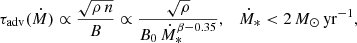 (B.1)
(B.1)
which is constant for Ṁ∗ ≥ 2 M⊙ yr−1,
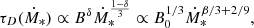 (B.2)
(B.2)
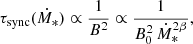 (B.3)
(B.3)
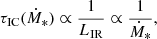 (B.4)
(B.4)
while τbrem, τion, and τpp are all  .
.
B.2. Model SEDs
We show the modelled SEDs for Ṁ∗ = 0.1 M⊙ yr−1 in the left panel of Fig. B.1. The dominant contribution at 150 MHz and 1.4 GHz comes from the synchrotron emission of primary electrons. In the case of Ṁ∗ = 10 M⊙ yr−1, which we show in right panel of Fig. B.1, the dominant contribution comes instead from synchrotron emission of secondary electrons. In both cases the free-free thermal component becomes important at higher frequencies. In the Fermi energy range the emission is dominated by hadronic emission for both SFRs.
B.3. The slope of the L1.4 GHz–SFR relation
In order to understand the behaviour of the slope η of Eq. (18) in the benchmark scenario, we approximate the electron distribution as a power law (N(E)=N0 E−p) in the electron-energy range producing the dominant synchrotron contribution to radiation at 1.4 GHz (ℰ1.4). This ranges between ∼1 GeV and ∼5 GeV for the benchmark scenario. Under this assumption, the synchrotron luminosity at a given frequency can be estimated roughly as  (Ghisellini 2013). For simplicity we focus on two typical values at low and high SFRs, where we can assume that electrons lose their energy through a single dominant process near ℰ1.4.
At low SFR  is shaped by primary synchrotron emission, and near Ṁ∗ = 0.1 M⊙ yr−1 the electron distribution is manly dominated by diffusion at ℰ1.4 ∼ 4 GeV (see upper left panel in Fig. 2). Then p = α + δ and N0,pri ∝ Ṁ∗τD, which results in
  . At high SFRs the slope of the primary electrons subdominant contribution can be estimated in a similar way taking into account that Bremsstrahlung dominates cooling. Then p = α, N0,pri ∝ Ṁ∗τbrem, and
  .
.
The emission of secondary electrons is dominant in  at high SFR. The normalisation of their particle distribution depends on the proton distribution roughly as
  (see Sect. 3.2), where τp and τe are the dominant loss times for protons and electrons, respectively.
Near Ṁ∗ ∼ 10 M⊙ yr−1 proton-proton interactions and advection dominate the proton losses, and Bremsstrahlung controls the electron cooling near ℰ1.4 (see lower right panel on Fig. 2). On the one hand, if we assume that proton-proton interactions dominate alone, then p = α,  , and
, and  . On the other hand, if we assume that advection domains alone, then
  , where
  . The combined effect of these two losses returns a dependence in SFR between these last two values.
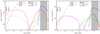 |
Fig. B.1. SEDs computed from scenario 0, for typical cases of low (Ṁ∗ = 0.1 M⊙/yr, left) and high (Ṁ∗ = 10 M⊙/yr, right) SFRs. The coloured lines (solid for the primary CRs and dashed for the secondary CRs) are the individual contributions of different non-thermal radiative mechanisms (the colour-coding is the same as in Fig. 2). The dashed brown line is the thermal free-free emission; the grey shaded region represents the Fermi-LAT energy range; and the vertical dotted black lines show the studied radio frequencies (150 MHz and 1.4 GHz). |
Appendix C: Hadronic processes
For the sake of completeness we report here the functions we adopted in the computation of all hadronic byproducts,
![Mathematical equation: $$ \begin{aligned} F_{\gamma }(x,E_p)= B_{\gamma } \frac{d}{dx} \Big [ \mathrm{ln}(x) \Big ( \frac{1-x^{\beta _{\gamma }}}{1+k_{\gamma }x^{\beta _{\gamma }}(1-x^{\beta _{\gamma }})} \Big )^4 \Big ] = \\ B_{\gamma } \frac{\mathrm{ln}(x)}{x} \Big ( \frac{1-x^{\beta _{\gamma }}}{1+k_{\gamma }x^{\beta _{\gamma }}(1-x^{\beta _{\gamma }})} \Big )^4 \times \nonumber \\ \Big [ \frac{1}{\mathrm{ln}(x)} - \frac{4 \beta _{\gamma } x^{\beta _{\gamma }}}{1-x^{\beta _{\gamma }}} - \frac{4 k_{\gamma } \beta _{\gamma } x^{\beta _{\gamma }} (1-2x^{\beta _{\gamma }})}{1+k_{\gamma }x^{\beta _{\gamma }}(1-x^{\beta _{\gamma }})} \Big ], \nonumber \end{aligned} $$](/articles/aa/full_html/2022/01/aa41295-21/aa41295-21-eq62.gif) (C.1)
(C.1)
where x = Eγ/Ep and
 (C.2)
(C.2)
 (C.3)
(C.3)
 (C.4)
(C.4)
and where L = ln(Ep/1 TeV);
![Mathematical equation: $$ \begin{aligned} F_e(x,E_p) = B_e\,\frac{[1+k_e(\mathrm{ln} x)^2]^3}{x(1+0.3/x^{\beta _e})} [- \mathrm{ln}(x)]^5, \end{aligned} $$](/articles/aa/full_html/2022/01/aa41295-21/aa41295-21-eq66.gif) (C.5)
(C.5)
where
 (C.6)
(C.6)
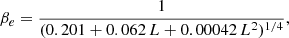 (C.7)
(C.7)
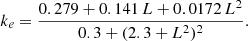 (C.8)
(C.8)
We also report the function  :
:
![Mathematical equation: $$ \begin{aligned} \tilde{f}_e(x)= f_{\nu _{\mu }^{(2)}}(x) = { g}_{\nu _{\mu }}(x) \, \Theta (x-r) + [h_{\nu _{\mu }}^{(1)}(x)+h_{\nu _{\mu }}^{(2)}(x)] \Theta (r-x), \end{aligned} $$](/articles/aa/full_html/2022/01/aa41295-21/aa41295-21-eq71.gif) (C.9)
(C.9)
where r = 1 − λ = (mμ/mπ)2 = 0.573,
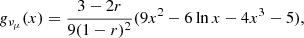 (C.10)
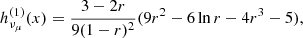 (C.11)
![Mathematical equation: $$ \begin{aligned} h^{(2)}_{\nu _{\mu }}(x) = \frac{(1+2r)(r-x)}{9\,r^2} \times [9\,(r+x)- 4 \,(r^2+rx+x^2)], \end{aligned} $$](/articles/aa/full_html/2022/01/aa41295-21/aa41295-21-eq74.gif) (C.12)
(C.12)
and Θ is the Heaviside step function.
All Tables
Distances, 1.4 GHz fluxes, 150 MHz fluxes, and luminosities for all γ-ray emitting SFGs known.
Values of the free parameters of our model (index of B(∗) relation, its normalisation, ionised gas fraction, temperature of the ionised gas) for all the scenarios considered.
All Figures
|
Fig. 1. Observed correlations for our galaxy sample. Upper left panel: L1.4 GHz as a function of the SFR. The blue solid line is the best fit to the data, and the shaded region its 68% confidence level. For comparison, the yellow dashed and green dotted lines show the Yun et al. (2001) and Bell (2003) relations, respectively. Upper right panel: L1.4 GHz as a function of LIR. The grey solid line is the best fit to the data, and the shaded region its 68% confidence level. For comparison, the green dotted line shows the Bell (2003) relation. Lower left panel: Lγ as a function of L1.4 GHz. The cyan solid line shows the best fit to the data, and the shaded region its 68% confidence level. For comparison, the brown dashed line shows the Ackermann et al. (2012) relation. Lower right panel: L150 MHz as a function of the SFR. The green solid line is the best fit to the data, and the shaded region its 68% confidence level. For comparison, the red dotted and violet dashed lines show the Gürkan et al. (2018) and Wang et al. (2019) relations, respectively. In all cases, the corresponding residuals weighted by their standard deviation are shown in the bottom panel; the black dotted lines correspond to 3σ. |
| In the text | |
|
Fig. 2. Cooling and escape times for primary electrons (upper panels) and protons (bottom panels) as a function of energy in scenario (0). Left panels: typical case of a low SFR galaxy (Ṁ∗ = 0.1 M⊙ yr−1). Right panels: typical case of a high SFR system (Ṁ∗ = 10 M⊙ yr−1). Solid lines represent different cooling processes: synchrotron (pink), ionisation (yellow), Bremsstrahlung (red), IC (green), and p − p (blue). The black dashed lines are for diffusion, whereas the grey double-dot-dashed lines are for advection. |
| In the text | |
|
Fig. 3. Lγ–SFR relation for scenario (0) using three different prescriptions for vadv: va (solid blue line), vsw (solid pink line), and vb from Eq. (15) (violet dashed line). The grey line and shaded band indicate the best fit to the data (purple circles) and its 1σ confidence region, respectively. The yellow region is forbidden by the calorimetric limit. |
| In the text | |
|
Fig. 4. Results for scenario (0) using vadv = vb from Eq. (15) (violet dashed line). Left panel: L1.4 GHz–SFR relation. The green dashed and dot-dashed lines represent the primary and secondary synchrotron electron contribution, respectively, and the dotted violet line the free-free contribution. The total emission at L1.4 GHz is also shown for two different prescriptions for vadv, vA (solid blue line) and vsw (solid pink line). Right panel: Lγ–L1.4 GHz relation. In both panels the grey shaded band indicates the 1σ confidence region of each fit (solid grey line) to the data sample (purple points). |
| In the text | |
|
Fig. 5. Model relations for the different scenarios considered (Table 2). The grey shaded band indicates the 1σ confidence region of each fit (grey solid line) to the data sample (purple points). In all panels the dotted lines represent the thermal emission, the dashed lines the non-thermal emission, and the solid line the total emission. Upper panel: for scenarios (0), (1), and (2) the L1.4 GHz–SFR relation (left) and the L1.4 GHz–LIR relation (right) are shown. Middle panel: for scenarios (0), (3), and (4) (left) and (0), (5), and (6) (right) the L1.4 GHz–SFR relation is shown. Bottom panel: for scenarios (0), (7), and (8) the L1.4 GHz–SFR relation (left) is shown and for scenarios (0), (5), and (6) the L150 MHz–SFR relation (right) is shown. |
| In the text | |
|
Fig. 6. L150 MHz–SFR relation obtained for scenario (0) using three different prescriptions for vadv: vA (solid cyan line), vsw (solid pink line), and vb from Eq. (15) (violet dashed line). The green dashed and green dot-dashed lines represent the primary and secondary electron contributions, respectively, and the dotted violet line represents the free-free contribution. The grey shaded band indicates the 1σ confidence region of the fit (solid grey line) to the data sample (purple points). |
| In the text | |
|
Fig. A.1. Stokes-I continuum image at 1.4 GHz for each galaxy in our sample. The flux scale is in Jy beam−1. The magenta contours indicate the 3σ level and the green solid contour the region selected for the flux integration. The synthesised beam is shown with a blue circle at the bottom left corner of each image. |
| In the text | |
|
Fig. B.1. SEDs computed from scenario 0, for typical cases of low (Ṁ∗ = 0.1 M⊙/yr, left) and high (Ṁ∗ = 10 M⊙/yr, right) SFRs. The coloured lines (solid for the primary CRs and dashed for the secondary CRs) are the individual contributions of different non-thermal radiative mechanisms (the colour-coding is the same as in Fig. 2). The dashed brown line is the thermal free-free emission; the grey shaded region represents the Fermi-LAT energy range; and the vertical dotted black lines show the studied radio frequencies (150 MHz and 1.4 GHz). |
| In the text | |
Current usage metrics show cumulative count of Article Views (full-text article views including HTML views, PDF and ePub downloads, according to the available data) and Abstracts Views on Vision4Press platform.
Data correspond to usage on the plateform after 2015. The current usage metrics is available 48-96 hours after online publication and is updated daily on week days.
Initial download of the metrics may take a while.