| Issue |
A&A
Volume 657, January 2022
|
|
|---|---|---|
| Article Number | A31 | |
| Number of page(s) | 16 | |
| Section | Catalogs and data | |
| DOI | https://doi.org/10.1051/0004-6361/202141168 | |
| Published online | 24 December 2021 | |
Detections of solar-like oscillations in dwarfs and subgiants with Kepler DR25 short-cadence data⋆
1
Instituto de Astrofísica de Canarias (IAC), 38205 La Laguna, Tenerife, Spain
e-mail: This email address is being protected from spambots. You need JavaScript enabled to view it.
2
Universidad de La Laguna (ULL), Departamento de Astrofísica, 38206 La Laguna, Tenerife, Spain
3
AIM, CEA, CNRS, Université Paris-Saclay, Université de Paris, Sorbonne Paris Cité, 91191 Gif-sur-Yvette, France
4
Department of Physics, University of Warwick, Coventry CV4 7AL, UK
5
Space Science Institute, 4765 Walnut Street, Suite B, Boulder, CO 80301, USA
6
LESIA, Observatoire de Paris, Université PSL, CNRS, Sorbonne Université, Université de Paris, 92195 Meudon, France
7
Institute for Astronomy, University of Hawai‘i, 2680 Woodlawn Drive, Honolulu, HI 96822, USA
8
Department of Astronomy, Columbia University, 550 West 120th Street, New York, NY, USA
9
Flatiron Institute, Simons Foundation, 162 Fifth Ave, New York, NY 10010, USA
Received:
23
April
2021
Accepted:
20
September
2021
Abstract
During the survey phase of the Kepler mission, several thousand stars were observed in short cadence, allowing for the detection of solar-like oscillations in more than 500 main-sequence and subgiant stars. These detections showed the power of asteroseismology in determining fundamental stellar parameters. However, the Kepler Science Office discovered an issue in the calibration that affected half of the store of short-cadence data, leading to a new data release (DR25) with corrections on the light curves. In this work, we re-analyzed the one-month time series of the Kepler survey phase to search for solar-like oscillations that might have been missed when using the previous data release. We studied the seismic parameters of 99 stars, among which there are 46 targets with new reported solar-like oscillations, increasing, by around 8%, the known sample of solar-like stars with an asteroseismic analysis of the short-cadence data from this mission. The majority of these stars have mid- to high-resolution spectroscopy publicly available with the LAMOST and APOGEE surveys, respectively, as well as precise Gaia parallaxes. We computed the masses and radii using seismic scaling relations and we find that this new sample features massive stars (above 1.2 M⊙ and up to 2 M⊙) and subgiants. We determined the granulation parameters and amplitude of the modes, which agree with the scaling relations derived for dwarfs and subgiants. The stars studied here are slightly fainter than the previously known sample of main-sequence and subgiants with asteroseismic detections. We also studied the surface rotation and magnetic activity levels of those stars. Our sample of 99 stars has similar levels of activity compared to the previously known sample and is in the same range as the Sun between the minimum and maximum of its activity cycle. We find that for seven stars, a possible blend could be the reason for the non-detection with the early data release. Finally, we compared the radii obtained from the scaling relations with the Gaia ones and we find that the Gaia radii are overestimated by 4.4%, on average, compared to the seismic radii, with a scatter of 12.3% and a decreasing trend according to the evolutionary stage. In addition, for homogeneity purposes, we re-analyzed the DR25 of the main-sequence and subgiant stars with solar-like oscillations that were previously detected and, as a result, we provide the global seismic parameters for a total of 525 stars.
Key words: asteroseismology / stars: solar-type / stars: activity / stars: rotation / stars: fundamental parameters / methods: data analysis
Full Tables 1–3, B.1, and E.1 are only available at the CDS via anonymous ftp to cdsarc.u-strasbg.fr (130.79.128.5) or via http://cdsarc.u-strasbg.fr/viz-bin/cat/J/A+A/657/A31
NSF Graduate Research Fellow.
© ESO 2021
1. Introduction
The NASA Kepler main mission has shown the power of using asteroseismology to precisely characterize the properties of solar-like stars (e.g., Silva Aguirre et al. 2017; Serenelli et al. 2017). Based on the latest catalogs of Kepler stellar properties (Huber et al. 2014; Mathur et al. 2017; Berger et al. 2018, 2020), more than 125 000 stars are purported to be main-sequence solar-like stars according to their effective temperatures, surface gravities as well as the results of their Gaia DR2 observations (e.g., Andrae et al. 2018; Gaia Collaboration 2018), which were included in the latest Kepler catalog. The turbulence of the outer layers of those stars excite oscillations that are known as solar-like oscillations (e.g., García & Ballot 2019). Given the radius, mass, and gravity of these stars, the modes are expected to be above 300 μHz, which means that we need to observe them in short cadence (sampling of ∼58.85 s) in order to detect the acoustic modes.
During the survey phase of the Kepler mission, around 2600 stars were observed between May 2009 and March 2010 for a duration of approximately one month each time and in a short-cadence mode. Chaplin et al. (2011a) performed a seismic analysis of the data available at that time and detected solar-like oscillations in more than 500 stars. This led to the seismic characterization of that sample, providing their masses, radii, and ages (Serenelli et al. 2017). More recently, Balona (2020) analyzed hot main-sequence stars with Teff > 6000 K in order to study the location of the δ Scuti/γ Doradus instability strip and detected solar-like oscillations in 70 new Kepler targets.
Subsequently, for the close-out of the nominal Kepler mission in 2016, a new data release (DR25, Thompson & Caldwell 2016)1 was carried out by the Kepler Science Office. The calibration of the data was improved, particularly with regard to how some instrumental effects were corrected, which had an impact on about half of the short-cadence data.
While the effect of the calibration should be negligible, the Kepler Science Office could not assess the impact on the asteroseismic studies. Using the newly calibrated data of DR25, Salabert et al. (2017a) re-analyzed the new light curves for 18 solar-analogs. In particular, these authors re-computed their global seismic parameters, such as the mean large frequency separation that scales with the root-mean-square of the mean stellar density (Kjeldsen & Bedding 1995) and the frequency of maximum oscillation power that is related to the surface gravity of the star (Brown 1991). Comparing the new results with those obtained with the previous data release (DR23), Salabert et al. (2017a) found that the impact on the measurement of the mean large frequency separation, the frequency of maximum oscillation power, and the background parameters was negligible for the stars with high signal-to-noise ratio (S/N). Nevertheless, the improvement in the light curve data could still have an impact on the detection of the modes. With this in mind, we conducted the current work to determine the impact of the improved DR25 on the mode detection for Kepler solar-like stars.
We would have hoped that the newly calibrated DR25 data would lead to a higher number of detections of solar-like oscillations. However, this does not take into account the surface magnetism of stars. Indeed, for the Sun and several solar-like stars, it has been shown that the amplitude of the modes is anti-correlated with magnetic activity (e.g., García et al. 2010; Howe et al. 2015; Kiefer et al. 2017; Santos et al. 2018). As a consequence, the non-detection of modes in the remaining stars can partially be explained by the high magnetic activity level of these stars (Chaplin et al. 2011b), along with other factors, such as metallicity or binarity, which may also be at play (Mathur et al. 2019).
In order to learn about the magnetic activity of stars with photometric data, we can use rotational modulation that results from the presence of active regions on the stellar surface. Additionally, the study of stellar rotation can provide key information for the understanding of angular momentum transport (e.g., Aerts et al. 2019; van Saders et al. 2019; Angus et al. 2020; Curtis et al. 2020; See et al. 2021). Several studies have been carried out on the basis of Kepler and K2 data to measure surface rotation periods in a large sample of stars (e.g., McQuillan et al. 2014; Santos et al. 2019, 2021; Reinhold & Hekker 2020; Gordon et al. 2021); furthermore, combined with the precise ages of stars, such as those obtained with asteroseismology or for clusters, it is possible to improve the general understanding of rotation-age relationships (e.g., Barnes 2003; Mamajek & Hillenbrand 2008; Angus et al. 2015; van Saders et al. 2016; Hall et al. 2021; Godoy-Rivera et al. 2021).
In Sect. 2, we describe the data we used in our study and the procedure for calibrating the light curves to optimize them for asteroseismic studies. In Sect. 3, we explain how the search for the acoustic modes was carried out and we consolidate the sample along with the stellar atmospheric parameters. Section 4 presents the study of the convective background parameters as well as the maximum amplitude of the modes and their correlation with the global seismic parameters. In Sect. 5, we compute the masses and radii based on the seismic scaling relations and in Sect. 6 we look at the rotation and magnetism of this new sample compared to the previously known sample of solar-like stars with detections of acoustic modes. Finally, we conclude with a discussion of the stellar parameters of the new seismic detections and we provide a summary of our work in Sects. 7 and 8.
2. Data description
In this work, we processed both the short-cadence (SC) data (sampling of 58.85s) and the long-cadence (LC) data (sampling of ∼29.42 min). The SC data were used for the asteroseismic analysis whereas the LC data were used for the study of the rotation and magnetic activity given that for those phenomena, a high cadence is not needed.
For the SC, the light curves used in this analysis are based on the last Kepler data release DR25, where the Kepler Science Office improved the calibration of the data. Indeed, as mentioned earlier, since the beginning of the mission, the short-cadence light curves were produced by correcting for the effects of Kepler shutterless readout. This scrambled the collateral smear and affected half of the short-cadence data. Hence, Presearch Data Conditioning – Simple Aperture Photometry (PDC-SAP; Jenkins et al. 2010) light curves were obtained from the Mikulski Archive for Space Telescopes (MAST)2.
The LC data were also obtained from the MAST but the calibrated light curves produced by the Kepler Science Office are not necessarily optimized for rotation studies as some filters are applied. Therefore, from the target pixel files, we first selected a larger aperture. Starting with the pixel of the center of the star, adjacent pixels are added to the aperture when the average flux of the new pixel is decreasing (i.e., new added pixels should have less flux than the previous one in each direction). The addition of pixels to the aperture is stopped if: (a) the mean flux of the new pixel increases, which suggests the presence of a nearby star; or (b) the mean flux of the new pixel is less than a given threshold, which is established at 100 e-/s. This threshold allows us to maximize the flux from the target and yields larger apertures than those employed for the standard PDC-SAP ones.
For both cadences, the obtained light curves were then calibrated for asteroseismology with the Kepler Asteroseismic Data Analysis Calibration Software (KADACS; García et al. 2011). We first removed outliers, corrected jumps, and removed instrumental trends. We also filled the gaps using the inpainting technique (with a multiscale discrete cosine transform), as described in García et al. (2014b) and Pires et al. (2015). This gap-filling technique allows us to reduce the noise at all frequencies, especially for light curves with rotation modulation. For the long-cadence light curves, we concatenated the different quarters and applied three high-pass filters with a cut-off period of 20, 55, and 80 days. Both the short-cadence and long-cadence corrected light curves, called KEPSEISMIC, are available on the MAST3.
In Fig. 1, we show the example of KIC 4484238, where the DR25 light curve leads to a significant improvement in the S/N. Indeed, while with the previous data release we could not detect any excess of power due to the oscillation modes, the DR25 power spectrum density (PSD) presents a bump around 2000 μHz. Finally, for the long-cadence data, we also used the Maximum A Posteriori (PDC-MAP, Thompson 2013) data, to which we applied the same KADACS correction software and gap-filling technique to check the rotation period retrieved from the light curves and to make sure that there is no nearby star polluting the aperture.
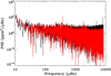 |
Fig. 1. Comparison of the Power Spectrum Density of KIC 4484238 using the DR24 data (black curve) and the DR25 data (red curve). |
3. Looking for new detections of solar-like oscillations
Using the short-cadence light curves calibrated in Sect. 2, we first performed a blind analysis of 2572 light curves with the A2Z pipeline (Mathur et al. 2010). This analysis provided global seismic parameters, in particular, the mean large frequency separation, Δν, and the frequency of maximum power, νmax. We then visually checked the stars for which the relation between Δν and νmax agreed within 20% of the empirical relation derived from the Kepler data (Huber et al. 2011). This led to a sample of 20 stars where the detection seemed to be clear. In addition, following the procedure of Mathur et al. (2010), we found that the measurement of Δν had more than 95% probability of being due to a stellar signal.
We then visually checked the outputs of the A2Z pipeline as well as the power spectrum densities of the remaining stars, flagging some clear detections as well as some candidates. We also computed the FliPer metric (Flicker in Power, Bugnet et al. 2018). We used the sklearn.ensemble.RandomForest Regressor function (Pedregosa et al. 2012) to train and combine predictions from a set of 200 independent random trees. By combining the effective temperature of the star (Huber et al. 2014 and Mathur et al. 2017, hereafter M17) and FliPer granulation parameters (see Bugnet et al. 2018, for more details about the intrinsic methodology and the training of the supervised machine learning algorithm), the trained Random Forest (Breiman 2001) provides rough estimates of the frequency of maximum power. Based on the power contained in the power spectrum, this procedure flags stars that have a power spectrum consistent with the ones of solar-like stars. This allowed us to select 20 additional stars for which the blind run of A2Z agreed within 20% of the FliPer predicted νmax.
For the remaining stars, we ran the A2Z pipeline again, forcing νmax to the predicted value from the FliPer metric. For that subsample, we selected the stars for which Δν agrees within 20% with the value expected from νmax, based on the seismic scaling relations.
These steps led to a total sample of 105 stars with possible or confirmed detections. After cross-checking with the sample of new detections by Balona (2020, hereafter Ba20), we added 43 stars to the analysis that had not been selected and that were part of our original sample. Our sample of 148 targets includes 60 stars that are part of the new detections of Ba20.
All the stars were also analyzed independently by the COR pipeline (Mosser & Appourchaux 2009), in a blind way first and then in an iterative way, consisting of using the seismic information provided by the νmax values derived by A2Z, in order to check for a possible agreement with this pipeline. We furthermore analyzed the sample with pySYD4 (Chontos et al. 2021), an open-source python-based adaptation of the SYD pipeline (Huber et al. 2009).
3.1. Consolidating surface gravity, effective temperature, and metallicity from the literature
In order to better characterize the stellar parameters, we consolidated the atmospheric parameters for the full sample of 148 stars by collecting values available in the literature. While all targets had log g, Teff, and [Fe/H] available from the M17, many of those values were obtained from photometry, which could have large uncertainties. However, since then, a few spectroscopic surveys have observed many of the targets in the Kepler field.
This is the case of the Apache Point Observatory for Galactic Evolution Experiment survey (APOGEE, Gunn et al. 2006; Wilson et al. 2019), which is part of the Sloan Digital Sky Survey-IV (SDSS-IV, Blanton et al. 2017) and which provides high-resolution spectroscopy for more than 15 000 Kepler targets. We used the DR16 (Ahumada et al. 2020) for which the data were calibrated following Holtzman et al. (2015), Nidever et al. (2015), and García Pérez et al. (2016). The majority of those stars were red giants, along with a few hundred of dwarfs and subgiants, as part of APOKASC (Serenelli et al. 2017; Pinsonneault et al. 2018), which is a collaboration between APOGEE and the Kepler Asteroseismic Science Consortium; however, they also included several thousands of dwarfs without seismic detections for other science objectives.
Another large spectroscopic survey, the Large Sky Area Multi-ObjectFiber Spectroscopic Telescope (LAMOST, Zhao et al. 2012; De Cat et al. 2015; Zong et al. 2018), also observed the Kepler field with low-resolution spectroscopy. Finally, the Gaia mission also provides precise parallaxes for a large sample of the Kepler field stars. Berger et al. (2020, hereafter B20) derived new stellar parameters for the Kepler-Gaia targets by fitting isochrones using the Gaia DR2 (Gaia Collaboration 2018).
We used the following prioritization to build our list of spectroscopic parameters for the 148 targets previously selected. When available, we first selected the stellar parameters obtained with high-resolution spectroscopy from APOGEE. Then we supplemented the parameters with low-resolution spectroscopy from LAMOST DR5 (Ren et al. 2018). Finally we took the stellar parameters from the latest Kepler-Gaia stellar parameters catalog. We found 102 stars with APOGEE spectra, 33 stars with LAMOST stellar parameters, and 13 stars with Gaia parameters.
3.2. Finalizing the sample of confirmed detections
The comparison of the results obtained by the three seismic pipelines (A2Z, COR, and pySYD) allowed us to build a list of confirmed detections constituted of 99 stars where at least two pipelines agree within 10% in νmax, as it has already been demonstrated that such scatter between pipelines is reasonable, particularly for low S/N cases (e.g., Zinn et al. 2020). In the remainder of the paper, we refer to those 99 stars as “our sample”.
The final step was to consolidate the values of the mean large frequency separation, Δν, which was more difficult to determine for the cases with very low S/N and low resolution. We visually checked the échelle diagrams of the 99 targets and found 19 stars where the value of Δν could be improved to have straighter ridges for the radial modes. So, we refined Δν by applying an additional analysis with the A2Z+ pipeline, where we created a template to mimic the modes with five orders when the initial value for Δν was taken as the value expected from scaling relations. We cross-correlated that template with the region of the PSD around νmax and swept the value of the mean large separation by +/−20%. The value for which we obtained the maximum correlation is taken as the new Δν. This allowed us to make a convergence for seven stars. For the remaining 12 stars (KIC 3124465, 5818478, 6289367, 7009852, 7255919, 7598321, 7708535, 8349736, 8652398, 9892947, 9894195, 9912680), we selected the Δν that straightened the ridges. The associated uncertainties for those stars were obtained by computing the difference between the selected value and the value obtained by the A2Z pipeline.
For the 60 stars in common with the sample of Ba20, we confirmed the seismic detections for 53 stars. The values of νmax of these stars are in agreement with the values reported by Ba20 within 10%. More specifically, there is an average offset of 4.3% in νmax, with a dispersion of 9.2%, and an average offset of 1.4% in Δν, with a dispersion of 4.1%. The mean large frequency spacings agree within 5%, except for KIC 7669332, which appeared as an outlier in Fig. 3 of Ba20. Our visual check of the échelle diagram confirms the reliability of our estimation. We also note that two targets of our sample (KIC 7215603 and 9715099) were included in Huber et al. (2013) and Chaplin et al. (2014, hereafter C14) but no νmax values were reported due to the aforementioned issue in the DR24.
We tested whether the apparent large fraction of stars that appear more massive than usually observed in previous seismic data sets could be related to any artifact due to, for instance, the low S/N of the detection. Any effect translating in an overestimation of νmax or underestimation of Δν will translate in an overestimated stellar mass derived from the seismic scaling relation. A general bias toward high νmax values is not expected for seismic data dominated by noise (Eq. (23) of Mosser et al. 2019). In order to identify any bias in Δν, we used the formalism developed by Mosser et al. (2013), which expresses the oscillation pattern in a parametric form. Therefore, we slightly smoothed the oscillation spectrum, with a smoothing function with a typical width of Δν/50, and correlated it with the generic oscillation pattern defined by Mosser et al. (2013). This allowed us to carry out a more precise measurement of the large separation, so that we can consider that the fraction of stars more massive than usually observed is real.
In Table 1, we provide the global seismic parameters as well as the atmospheric parameters of the 99 stars with confirmed detection of solar-like oscillations. Figure 2 represents the seismic Hertzsprung-Russell Diagram of the Kepler solar-like stars for which C14 had detected oscillations (grey symbols) along with the new confirmed detections (red symbols). We can see that many of the stars in our sample are hotter than the Sun, hence, those that are more on the massive side, as well as more evolved solar-like stars, with a large proportion of subgiants. We also populate more the early red giant region where C14 had reported around tens of such evolved stars.
Seismic and stellar parameters of the 99 stars with seismic detections.
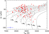 |
Fig. 2. Seismic Hertzsprung-Russell Diagram where the mean large frequency separation is used instead of the luminosity. The C14 solar-like stars are represented with grey circles where the effective temperature is taken from the M17. The 99 stars with confirmed seismic detections are shown with red squares where the effective temperature is coming from APOGEE, LAMOST or B20 (see Sect. 3.1). The position of the Sun is indicated by the ⊙ symbol and the grey solid lines represent evolution tracks from ASTEC (Christensen-Dalsgaard 2008) for a range of masses at solar composition (Z⊙ = 0.0246). Typical uncertainties are represented in the bottom left corner. |
We note that six of our targets have been flagged as “BinDet_NoCorr” in the B20 catalog, suggesting that they are binary candidates, which will have an impact on the derived effective temperature towards the red. We looked for the Gaia DR2 effective temperatures of those stars. For four of them, the values agree with those reported in the spectroscopic surveys, within the uncertainties. For one star, there is no Gaia DR2 Teff. For the target KIC 3633538, the Gaia effective temperature is 5676 K, compared to 5100 K in B20. The lower temperature in B20 can be explained by the binarity, so we used the Gaia effective temperature for that star. This higher value is also more compatible with the location of the solar-like oscillation modes for that star.
The results of the global seismic analysis are shown in a Δν–νmax diagram (Fig. 3) for the stars in our sample (red squares) to be compared to the C14 sample (grey circles). We can see that the relations are very similar. Nevertheless, we can also note some of the stars in our sample below the general trends, in particular near νmax of 500 μHz, suggesting that those stars are slightly more massive than the rest of the sample, which was shown for instance by Mosser et al. (2010). The average uncertainties are of 2.4% in νmax and 5.8% on Δν. The latter is slightly high compared to the usually 5% reported in C14 but representative of the low S/N.
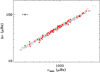 |
Fig. 3. Mean large frequency spacing, Δν, as a function of the frequency of maximum power, νmax for the C14 sample (grey circles) and our sample (red squares). Typical uncertainties are shown in the upper left corner. |
Using the surface gravity and effective temperature in the seismic scaling relations, we can estimate a predicted value for the frequency of the maximum power as follows:
 (1)
(1)
where νmax, ⊙ is the frequency of maximum power for the Sun, taken as 3100 μHz, Teff, ⊙= 5777 K, and log g⊙ = 4.4377 dex.
In Fig. 4, the measured νmax for the confirmed sample is compared to the predicted value, νmax, pred from Eq. (1). Here we used the log g from B20, as these values have been shown to be more reliable. The B20 catalog contains 186 301 Kepler stars and a surface gravity value was available for 97 of our stars. The agreement between the observed and the predicted νmax is in general within 20% with an average discrepancy of 1.2%, with the predicted νmax overestimating the observed one. However, the disagreement can reach up to 50%.
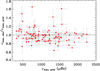 |
Fig. 4. Ratio of the observed νmax, obs and the predicted νmax, pred using the log g from B20. The dashed line shows the equality of both values. |
We made a similar comparison by using the spectroscopic surface gravities (see Appendix A) and the disagreement is larger with an average discrepancy of 30% – again, with an overestimation of the prediction.
We note that around 10 of the stars have a high-enough S/N to fit the individual modes. The determination of the frequencies of the individual modes will allow us to do boutique modeling for that subsample of stars, which will provide more precise stellar parameters as well as ages. This exercise is beyond the scope of this paper and is part of a subsequent paper (Mathur et al., in prep.).
We also visually checked the échelle diagrams of the remaining 49 stars of the 148 stars without confirmation of acoustic-mode detection. A list of candidates of 26 stars was retained, where either the échelle diagram seemed to show some ridges, though with a very poor S/N, or when there was some agreement with the predicted νmax. We note that some of these candidates did not necessarily have an agreement between pipelines and three of them are part of the Ba20 sample. We show the properties of those candidates in the Appendix B.
Finally, we re-analyzed the C14 sample using the DR25, providing a homogeneous catalog with the global seismic properties of the main-sequence and subgiant stars with the detection of solar-like oscillations observed in short-cadence during the survey phase of the Kepler mission (see Table 2). To that sample, we also added a few tens of stars from Campante et al. (2011), Mathur et al. (2011a), Appourchaux et al. (2012, 2015), White et al. (2017). In 19 stars, we realized that the SAP aperture of the new DR25 is not appropriate for asteroseismic studies because they were too small (2 or 3 pixels). By applying the same aperture extraction methodology described in this paper for the LC dataset, we were able to reduce the noise level of the resultant light curve and the modes were detectable. In total, we detected the modes for 525 stars with 514 stars in common with the C14 sample. As shown by Salabert et al. (2017a) who analyzed a subsample of solar analogs with DR23 and DR25, for the high S/N targets, the global seismic parameters remain the same. The values reported by C14 and the A2Z results with the DR25 have a median offset of 0.5% in νmax and of 0.2% in Δν. We note that we also report νmax values for 34 stars that were in C14, but for which only Δν was provided and no νmax was given. We do not report the seismic parameters for 4 stars from C14 as we could not detect any solar-like oscillations.
Global seismic parameters from A2Z for the 525 stars with previous detection of solar-like oscillations.
4. Granulation and modes amplitudes
The determination of the global seismic parameters provides invaluable information on the convective parameters of the solar-like stars as well as the maximum amplitude of the modes. It has been shown that there are tight relations between these parameters and the frequency of maximum power of the acoustic modes (e.g., Huber et al. 2011; Mathur et al. 2011b; Mosser et al. 2012; Kallinger et al. 2014). Here, we study these parameters and compare them with the known sample of solar-like stars with detected oscillations. This comparison allows us to check any deviation from those known relations.
4.1. Convective background parameters
The study of a large number of stars with solar-like oscillations from the main sequence to the red-giant branch showed that the convective background parameters are correlated with the location of the modes and follow scaling relations (Kjeldsen & Bedding 2011; Mathur et al. 2011b; Kallinger et al. 2014).
The background fit was performed with a Monte Carlo Markov chains (MCMC) strategy using the apollinaire module5 (Breton et al., in prep.), which uses the emcee package (Foreman-Mackey et al. 2013). For the fit, we considered the PSD above 5 μHz. The model is composed of four components: a power law for the magnetic activity, two Harvey models (Harvey et al. 1985) for different scales of granulation, and the photon noise at high frequency. All the results have been visually inspected and some PSD were fitted again with a frequency cut at 50 μHz. For that higher frequency cut, the fitted model was only constituted of two Harvey models and a flat noise profile. The Harvey law fitted has the form:
 (2)
(2)
where Pgran is the granulation power, νgran is the characteristic frequency, and the slope α is fixed to 4 following Kallinger et al. (2014). Pgran is related to the granulation amplitude as the  per frequency bin.
Figure 5 shows the granulation frequency for the second Harvey model of convection (the one below the modes), νgran (top panel), and the granulation power, Pgran (bottom panel), as a function of νmax. The grey points represent the values for a subsample of 163 stars from the C14 sample. The analysis of that subsample was also done with the apollinaire pipeline on data calibrated with the KADACS software that generated the KEPSEISMIC light curves. This allows us to directly compare the parameters of the stars in our sample with those of C14. We can see in both plots that the new confirmed detections have the convective parameters in the same range as the known oscillating solar-like stars and have similar trends following the relations derived for stars from the main sequence to the red-giant branch (Kallinger et al. 2014), shown with blue dashed lines. For Pgran, we used the power law relation with a slope of 2.1, as given in Sect. 5.4 of Kallinger et al. (2014).
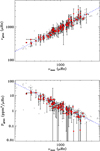 |
Fig. 5. Granulation frequency (top panel) and power (bottom panel) as a function of the frequency of maximum power. The stars in our sample are represented with red squares while the subsample of 163 stars from C14 are represented with grey circles. The blue dashed lines are the relations derived by Kallinger et al. (2014). |
4.2. Maximum amplitude of the modes
From the Gaussian fit around the region of the modes, we derived the bolometric maximum amplitude of the modes following conversion of Kjeldsen et al. (2008) and Ballot et al. (2011). For three stars, namely KIC 3633538, 9529969, and 10340511, the Gaussian fit could not converge due to the low S/N and did not provide the maximum amplitude of the modes. However, a value for the frequency of maximum power was obtained from the maximum around the region of the modes in the power spectrum density that was smoothed with a boxcar average of width of 2 × Δν.
In Fig. 6, we can see here again that the stars in our sample have a similar behavior as compared to the C14 sample. We note that for the most evolved stars of our sample – evolved subgiants with νmax down to 500 μHz and early red giants with lower νmax (see Fig. 1 of Mosser et al. 2014) – Amax is closer to the lower edge. The blue dashed line corresponds to the fit of the form of a power law between Amax and νmax for the C14 sample. We find  . These lower amplitudes combined with the noisier DR24 data, could explain the difficulty to detect the modes in the early analysis of those targets by Chaplin et al. (2011a).
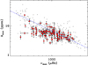 |
Fig. 6. Bolometric maximum amplitude of the modes as a function of νmax. The legend is the same as in Fig. 5. The blue dashed line corresponds to the fit for the stars from C14. |
5. Global stellar parameters
Using the seismic scaling relations (Brown 1991; Kjeldsen & Bedding 2011), we computed the masses and radii of our sample where we combined the global seismic parameters and the atmospheric parameters from Sect. 3.1 as follows:
 (3)
(3)
 (4)
(4)
where νmax, ⊙ = 3100 μHz and Δν⊙ = 135.2 μHz.
Among the confirmed detections, 79 stars have APOGEE spectroscopic parameters and 16 have LAMOST values. The remaining 4 stars have Teff and [Fe/H] from the Gaia-Kepler catalog.
In Fig. 7, we represent the mass-radius diagram with our sample with red squares and the previously known sample of solar-like stars with oscillation detections in Kepler with grey circles. For the latter sample, the masses and radii were computed by Serenelli et al. (2017, hereafter S17) who used grid-based modeling where the global seismic parameters (Δν and νmax) were combined with spectroscopic observables (Teff, log g, and [Fe/H]). We can see that our new sample includes a larger fraction of massive stars, as suggested above.
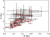 |
Fig. 7. Radius versus mass diagram for the C14 stars using S17 parameters (grey circles) and the stars in our sample described in this work (red diamonds). For the latter, corrections on Δν were applied following Mosser et al. (2013). |
Given that the observed Δν might not be obtained in the asymptotic regime as it should be measured in a frequency range above νmax, several approaches have been developed to apply a correction on the observed mean large frequency separation in order to reduce the impact on the derivation of the stellar masses and radii (e.g., White et al. 2011; Mosser et al. 2013; Guggenberger et al. 2016; Sharma et al. 2016; Kallinger et al. 2018; Benbakoura et al. 2021). For instance, Mosser et al. (2013) derived an empirical correction by taking into account the second-order term in the Tassoul relation (Tassoul 1980) and by using seismic observations for main-sequence to red-giant stars. The approach by Sharma et al. (2016) used a grid of models of red giants where the mean large frequency from the sound speed profile was compared to the one obtained by using the computed frequencies, leading to a grid of Δν corrections for each model of the grid. Given that our targets have a rather small S/N and that they are main-sequence stars and subgiants, we decided to adopt the Mosser et al. (2013) corrections. They led to smaller radii by 1.5% on average and smaller masses by 2.9% on average compared to the radii and masses obtained without Δν corrections.
In Fig. 7, we can see that 2 stars have masses above 2 M⊙, which was not expected in our sample as they are in the instability strip and do not have an external convective envelope needed for the excitation of solar-like oscillations (Aerts et al. 2010). Given the high uncertainties on the seismic parameters, which are reflected by the larger error bars for those stars, they could be attributed to the low S/N of the modes.
6. Rotation and magnetic activity
For the 99 stars with a confirmed detection of solar-like oscillations, we analyzed the long-cadence time series to look for the surface rotation periods and measure the level of magnetic activity. These measurements are based on the presence of active regions or spots that come in and out of view and lead to a modulation in the light curves that is related to the surface rotation. For this analysis, we applied three different techniques: a time-frequency analysis based on wavelets (Torrence & Compo 1998; Liu et al. 2007; Mathur et al. 2010), the auto-correlation function (García et al. 2014a; McQuillan et al. 2014), and the composite spectrum that combines the two previous methods (Ceillier et al. 2016, 2017; Santos et al. 2019). The reliable rotation periods, Prot, were selected following criteria described in Santos et al. (2019, 2021), and Breton et al. (2021). Briefly, we use the three different filtered KEPSEISMIC light curves to select the rotation period. We then use the PDC-MAP light curves to confirm that the rotational signal does not result from pollution (instrumental or stellar) as the KEPSEISMIC light curves have a larger aperture compared to the PDC-MAP and are calibrated without taking into account the information on the instrumental drifts embedded in the co-trending basic vectors used in PDC-MAP. We should note that PDC-MAP light curves are often filtered at 20 days and, in Santos et al. (2019), we showed that solely by using PDC-MAP light curves, the distribution of retrieved rotation periods is shifted toward shorter values. When the rotation periods inferred from both calibration systems agree inside the combined errors, they are less likely to come from some instrumental pollution or pollution by nearby stars. Some examples of light curves are shown in Appendix D. We obtained surface rotation periods for 63 stars (see Table 3), among which one was classified as a close binary candidate, based on the fast rotation and the shape of the light curve (See Santos et al. 2019, 2021, for more details).
Rotation periods and magnetic activity levels of the 63 stars with seismic detections.
For stars with rotation period measurements, we computed the photometric magnetic index, Sph, following Mathur et al. (2014). Briefly, we first calculate the standard deviation of subseries of length 5 × Prot and compute the mean value. This index has been shown to provide a relevant proxy for magnetic activity based on the Sun and a few solar-like stars and comparison with classical magnetic activity indexes (Salabert et al. 2016, 2017b).
In Fig. 8, we represent Prot as a function of the effective temperature of the stars for the new seismic detections and the sample of García et al. (2014a, hereafter G14). The stars with new seismic detection seem to be quite homogeneously distributed. While we noticed that a significant fraction of those stars are in their subgiant phase, very few stars have long rotation periods. Because stars spin-down as they evolve (e.g., Skumanich 1972; Kawaler 1988; Gallet & Bouvier 2013), a greater number of slow-rotating (Prot > 40 days) subgiants were expected in comparison with what was found in this study. However, many of the subgiants of our sample are generally more massive than 1.2 M⊙, which corresponds to the Kraft break (Kraft 1967). Stars above the Kraft break do not undergo magnetic braking due to stellar winds – in contrast to the lower mass stars. This difference between the high-mass and low-mass solar-like stars could explain the rotation periods retrieved for our sample.
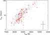 |
Fig. 8. Surface rotation periods, Prot, as a function of effective temperature, Teff, for the G14 sample (grey circles) and our sample (red squares). Typical error bars are shown in the bottom right corner. |
7. Discussion
Here, we look at the different properties of the stars with detections of solar-like oscillations presented in this paper and compare them to the C14 sample, in particular, to investigate a possible gain in the parameter space that we are probing.
7.1. Magnitude distribution
We first looked at the magnitude of the targets. Indeed, in addition to the calibration issue of the data, the previous non-detection of the modes for those stars could also be affected by higher photon noise that depends on the stellar magnitude. The higher noise in the data could lead to a non-detection. Figure 9 shows the distribution of the Kepler magnitude, Kp, for our sample and the C14 sample. While they probe a similar range of magnitudes, we can see that the stars in our sample have a larger fraction of stars fainter than 11 compared to the C14 sample. We find that 55.5% of the stars in our sample have Kp > 11, compared to 39% for the C14 sample.
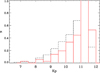 |
Fig. 9. Normalized histogram of the Kepler magnitude for the C14 sample (black dashed line) and our sample (red solid line). |
We perform a Kolmogorov-Smirnov test to quantify the comparison of the distribution of the magnitudes between the C14 sample and our sample of new seismic detections. We find a deviation value of 0.22 as well as a probability on the distributions differences of 0.05%, which means that the magnitudes distributions are indeed very different. This confirms the finding that our sample with detections of solar-like oscillations presented in this paper are fainter.
7.2. Blends explaining the previous non detections
With these detections of solar-like oscillations in our sample using the new DR25, we may wonder whether the previous non-detection was related to the presence of nearby stars. To check for that possibility, we cross-matched the list of stars in our sample with Gaia EDR3 (Gaia Collaboration 2021) and checked two possible sources of amplitude dilution: (1) companions that are unresolved by Gaia, as indicated by high Gaia RUWE (Renormalized Unit Weight Error) values (RUWE > 1.4 typically indicates binaries). While the contrast between the main star and the companions is not known, it is possible that a pollution can arise; (2) all resolved stars in Gaia within 20″(5 Kepler pixels) of the target. For stars with multiple companions, we selected the brightest star within the search radius.
From that analysis, we find 15 stars where RUWE > 1.4 and 9 stars for which the magnitude difference between our target and the brightest star within 20″ is smaller than 3. So, 24 stars are flagged to have a nearby star that may dilute the amplitude of the flux and could have prevented the detection of the modes. This number represents an upper limit of the number of stars for which oscillations could not be detected due to a blend. We also checked the amplitude of the modes for those stars that we flagged and found that 7 of them have a lower amplitude of the modes, which can thus be explained by the possible blends. For the remaining 22 stars without a nearby polluting star, it is very likely that the better quality of the data allows us to detect the modes presented in this paper.
7.3. Metallicity distribution
Metallicity can play a role on the detectability of solar-like oscillations as was shown by Samadi et al. (2010). Indeed, they suggested that for metal-poor stars, the amplitude of the modes was decreased. Figure 10 shows the distribution of the metallicity for the 95 stars of our sample (red solid line), where [Fe/H] comes from either APOGEE or LAMOST as metallicity from B20 is not as reliable. We can see that it peaks at solar metallicity. For comparison the metallicity distribution of the C14 sample is represented on the same figure with the dashed line, also peaking at solar metallicity. We note that among the stars in our sample, 51% of them are metal poor compared to the Sun while 54% of the C14 sample are metal poor but given the typical uncertainties of 0.1dex the difference does not seem significant. We quantify the differences between the distributions of the two sample using a Kolmogorov-Smirnov test. We obtain a deviation of 0.08 with a probability that one sample is different from the other of 62.4%, confirming that the distributions are not significantly different.
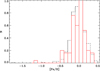 |
Fig. 10. Normalized histogram of the Kepler metallicity for the C14 sample (black dashed line) and for our sample (red solid line) for the 95 stars with new seismic detections and with APOGEE or LAMOST spectroscopic observations. |
7.4. Surface magnetic activity
As explained in Sect. 6, from the photometric activity proxy, Sph, we can also investigate whether the stars with of our sample have different levels of magnetic activity compared to G14. In Fig. 11, we show the magnetic activity index Sph as a function of the rotation period Prot for the stars from G14 with reliable rotation periods and for which asteroseismic detection had been obtained (grey circles). The results for the stars in our sample are shown with the red squares and the close binary candidate with a blue square. We can see that most stars with detected oscillations have similar Sph values that are in the same range as the solar ones between the minimum and maximum of its magnetic cycle as computed in Mathur et al. (2019) (delimited by the dashed lines). There are some stars with magnetic activity levels above the range of the solar cycle for both the previously known sample and our sample. However, the new sample of this work adds four stars that are slower rotators (Prot ≥ 30 days) and with high Sph values. We also note that one star (KIC 8165738) has a very low Sph value of ∼10 ppm. The modulation appears to be factual. We recall that since we do not have the inclination angles of the rotation axis of the stars, the Sph values that we measure are a lower limit of the real magnetic activity level.
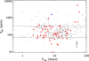 |
Fig. 11. Magnetic activity proxy, Sph vs surface rotation period, Prot for the G14 sample (grey circles) and our sample (squares). The blue square is the close binary candidate, KIC 4255487. The dashed lines correspond to the Sph values between minimum and maximum magnetic activity from Mathur et al. (2019). The typical error bars are represented in the bottom right-hand side. |
Among those stars, three are flagged as potential binary systems as discussed in Sect. 3.2 (KIC 3633538, KIC 777146, KIC 10969935).
7.5. Radius comparison with Gaia DR2
As shown in Sect. 3.1, the Kepler-Gaia stellar properties catalog made use of the Gaia DR2 in order to improve the stellar parameters of the Kepler targets by using the new precise parallaxes measurements. In B20, isochrones were fitted using spectroscopic and photometric information available from previous catalogs and combined them with the Gaia data. As stated earlier in this paper, 97 of our solar-like stars with new seismic detections are included in the B20 catalog.
We find a general agreement between the seismic radii, Rseis and the Gaia radii, RGaia, for both our sample (left panel of Fig. 12) and the S17 sample (right panel of Fig. 12) for comparison. For more clarity in the figure, we represent the S17 sample without the uncertainties. In our sample, we note that for larger stars (radii above ∼2.5 R⊙), hence, more evolved stars, the seismic radii uncertainties become larger, due to larger uncertainties on the seismic parameters in comparison with smaller stars. We find that in average the Gaia radii are overestimated compared to the seismic ones by 4.4%, with a scatter of 12.3%. A general trend can be seen, where with increasing seismic radii RGaia/Rseis decreases. For main-sequence stars, the average disagreement is of 10.2%, where the seismic radii are underestimated compared to the Gaia radii. For subgiants with radii between 1.5 and 3 R⊙, we find that the seismic radii are underestimated by 3.3% on average. Finally, for early red giants with radii above 3 R⊙, the seismic radii are overestimated by 1.2% on average.
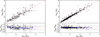 |
Fig. 12. Left panel: comparison between the seismic radii after applying the Mosser et al. (2013) corrections on Δν and the Gaia radii (top panel) and ratio of the radii for our sample (bottom panel). The blue squares represent the median binned data. Only 97 stars are shown as two targets do not have a Gaia radius. Right panel: same details but for the S17 sample. |
These results are slightly different from what was found by Huber et al. (2017), where a similar comparison was done on a larger sample of stars from the main sequence to the red giants but using the Tycho-Gaia astrometric solution (Michalik et al. 2015; Gaia Collaboration 2016). Their sample included the previously known solar-like stars with a detection of acoustic modes. They found a disagreement of 5% for radii between 0.8 and 8 R⊙, where seismic radii for dwarfs and subgiants were underestimated compared to Gaia radii. Later Sahlholdt & Silva Aguirre (2018), Khan et al. (2019), and Zinn et al. (2019) looked at differences between Gaia radii obtained with DR2 and the seismic ones, for dwarfs and red giants. For red giants, Khan et al. (2019) reported a 2% discrepancy between the seismic and astrometric radius and showed how stellar radii can be calibrated with Kepler and Gaia (see their Figs. 17 and 19). For dwarfs, Sahlholdt & Silva Aguirre (2018) and Zinn et al. (2019) found that the seismic radii were underestimated compared to the Gaia ones by 2%. In particular, Zinn et al. (2019) investigated random and systematic uncertainties related to luminosity, effective temperatures, bolometric corrections and estimated the systematic uncertainties to be around 2% as well. Our findings for the new seismic detections show larger discrepancies. Taking the systematics errors, the results obtained for the new seismic detections are thus consistent with the previously known solar-like stars when using Gaia DR2.
To check wether any of the bias or trends between seismic radii and radii inferred with Gaia observations are due to any effect of the effective temperature scale, we compute the seismic radii using the effective temperatures from B20. We find that on average the Gaia radii are overestimated by 3.3% with a scatter of 12.4%. Using the effective temperatures from B20 should bring the discrepancy closer to 0. Thus, the difference that remains here is likely to be related to the input from the global seismic parameters (see Appendix E).
Finally, in order to better assess the agreement between the two ways of obtaining the stellar radii, we compare the radii differences as a function of the combined uncertainties from both seismology and Gaia (see Fig. 13). For 50.5% of the stars, the differences between the two methodologies are within 1σ.
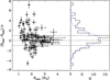 |
Fig. 13. Left panel: Differences between the Gaia radius and the seismic radius in units of the statistical uncertainty (σ), computed as the quadratic sum of the uncertainties from the B20 radii and the scaling relations radii. Right panel: histogram of the same differences. Dashed lines show the equality of both radii and the dot-dash lines represent the ±1σ limits. Only 97 stars are shown as two targets do not have a Gaia radius. The blue dashed line shows a Gaussian fit of the histogram. |
8. Conclusions
We analyzed the light curves from the latest data release of the Kepler mission for about 2600 stars that were observed in short cadence for one month during the survey phase of the mission. We obtained reliable seismic detections for 99 solar-like stars, among which there are 46 stars with newly reported detections. Our analysis increased, by more than 15%, the number of Kepler dwarfs with a full seismic study. We also re-analyzed the DR25 of the sample of stars with previously detected modes by C14 and provide a homogeneous catalog of global seismic parameters for additional 525 main-sequence and subgiant stars observed by Kepler during the survey mission, yielding a homogeneous seismic properties catalog for 624 stars for which a complete table of the global seismic parameters are given in Appendix E.
For the full sample, we consolidated atmospheric parameters from APOGEE, LAMOST, and the Kepler-Gaia catalogs. Using the surface gravity and effective temperature from the Kepler-Gaia catalog, we predicted frequency of maximum oscillation power of the modes based on seismic scaling relations. We found that, on average, the predicted νmax is slightly higher than the observed one.
The computation of the seismic masses and radii from the scaling relations and with the Mosser et al. (2013) corrections on the mean large frequency spacing suggests that our target stars are, on average, more massive and off the main sequence, as compared to the existing Kepler dwarfs and subgiants in the literature.
While the background parameters have similar trends with νmax as previously found in the literature, the maximum amplitude of the modes appears to be on the lower end of the known trends. We also found that the sample of new seismic detections is constituted of fainter stars, which can lead to lower amplitude of the modes. This could partly explain the non detection of the acoustic modes for those stars when using the DR24 that was affected by some calibration issues concerning the short-cadence data of Kepler. Both our sample and the sample of Chaplin et al. (2014) exhibit, on average, a solar metallicity.
By using Gaia data to look for stars close to our targets, we found that 7 of the stars with detections of solar-like oscillations in our sample have a nearby companion that may pollute the observations. This could explain the non detections of acoustic modes with the previous Kepler data releases.
From the analysis of the surface rotation of the light curves, we obtained reliable rotation periods for 63 stars. These stars have magnetic activity levels in the same range as the Sun along its activity cycle. Even though the sample that features new seismic detections has a larger number of subgiants, we did not find many slow rotators. This is probably because these are massive subgiants that are above the Kraft break on the main sequence and have not gone through strong magnetic braking.
Finally, we find that seismic radii are, on average, 4.4% underestimated compared to the Gaia DR2 radii with a scatter of 12.3% and a decreasing trend with evolutionary stage, which is in agreement with previous comparisons done for main-sequence to red-giant stars. Using a different scale of temperature from the Kepler-Gaia catalog, the discrepancy slightly decreased.
Many of the stars with new seismic detections have a very low S/N, however, around ten of them could have their individual modes characterized, which will be part of a subsequent paper. Even though Kepler stopped operating more than five years ago, the high precision and continuous data collected by the mission still represent a goldmine for asteroseismology.
The source code is available at https://gitlab.com/sybreton/apollinaire
Acknowledgments
This paper includes data collected by the Kepler mission. Funding for the Kepler mission is provided by the NASA Science Mission directorate. Some of the data presented in this paper were obtained from the Mikulski Archive for Space Telescopes (MAST). STScI is operated by the Association of Universities for Research in Astronomy, Inc., under NASA contract NAS5-26555. S. M. acknowledges support by the Spanish Ministry of Science and Innovation with the Ramon y Cajal fellowship number RYC-2015-17697 and the grant number PID2019-107187GB-I00. R. A. G. and S. N. B acknowledge the support from PLATO and GOLF CNES grants. A. R. G. S. acknowledges the support from National Aeronautics and Space Administration under Grant NNX17AF27G and STFC consolidated grant ST/T000252/1. D.H. acknowledges support from the Alfred P. Sloan Foundation, the National Aeronautics and Space Administration (80NSSC19K0597), and the National Science Foundation (AST-1717000). M.S. is supported by the Research Corporation for Science Advancement through Scialog award #26080. Guoshoujing Telescope (the Large Sky Area Multi-Object Fiber Spectroscopic Telescope LAMOST) is a National Major Scientific Project built by the Chinese Academy of Sciences. Funding for the project has been provided by the National Development and Reform Commission. LAMOST is operated and managed by the National Astronomical Observatories, Chinese Academy of Sciences.
References
- Aerts, C., Christensen-Dalsgaard, J., & Kurtz, D. W. 2010, Asteroseismology (Springer Science+Business Media B.V.) [Google Scholar]
- Aerts, C., Mathis, S., & Rogers, T. M. 2019, ARA&A, 57, 35 [Google Scholar]
- Ahumada, R., Allende Prieto, C., Almeida, A., et al. 2020, ApJS, 249, 3 [NASA ADS] [CrossRef] [Google Scholar]
- Andrae, R., Fouesneau, M., Creevey, O., et al. 2018, A&A, 616, A8 [NASA ADS] [CrossRef] [EDP Sciences] [Google Scholar]
- Angus, R., Aigrain, S., Foreman-Mackey, D., & McQuillan, A. 2015, MNRAS, 450, 1787 [Google Scholar]
- Angus, R., Beane, A., Price-Whelan, A. M., et al. 2020, AJ, 160, 90 [Google Scholar]
- Appourchaux, T., Chaplin, W. J., García, R. A., et al. 2012, A&A, 543, A54 [CrossRef] [EDP Sciences] [Google Scholar]
- Appourchaux, T., Antia, H. M., Ball, W., et al. 2015, A&A, 582, A25 [NASA ADS] [CrossRef] [EDP Sciences] [Google Scholar]
- Ballot, J., Barban, C., & van’t Veer-Menneret, C. 2011, A&A, 531, A124 [NASA ADS] [CrossRef] [EDP Sciences] [Google Scholar]
- Balona, L. A. 2020, Front. Astron. Space Sci., 7, 85 [NASA ADS] [CrossRef] [Google Scholar]
- Barnes, S. A. 2003, ApJ, 586, 464 [Google Scholar]
- Benbakoura, M., Gaulme, P., McKeever, J., et al. 2021, A&A, 648, A113 [NASA ADS] [CrossRef] [EDP Sciences] [Google Scholar]
- Berger, T. A., Huber, D., Gaidos, E., & van Saders, J. L. 2018, ApJ, 866, 99 [NASA ADS] [CrossRef] [Google Scholar]
- Berger, T. A., Huber, D., van Saders, J. L., et al. 2020, AJ, 159, 280 [Google Scholar]
- Blanton, M. R., Bershady, M. A., Abolfathi, B., et al. 2017, AJ, 154, 28 [Google Scholar]
- Breiman, L. 2001, Mach. Learn., 45, 5 [Google Scholar]
- Breton, S. N., Santos, A. R. G., Bugnet, L., et al. 2021, A&A, 647, A125 [EDP Sciences] [Google Scholar]
- Brown, T. M. 1991, ApJ, 371, 396 [NASA ADS] [CrossRef] [Google Scholar]
- Bugnet, L., García, R. A., Davies, G. R., et al. 2018, A&A, 620, A38 [NASA ADS] [CrossRef] [EDP Sciences] [Google Scholar]
- Campante, T. L., Handberg, R., Mathur, S., et al. 2011, A&A, 534, A6 [NASA ADS] [CrossRef] [EDP Sciences] [Google Scholar]
- Ceillier, T., van Saders, J., García, R. A., et al. 2016, MNRAS, 456, 119 [Google Scholar]
- Ceillier, T., Tayar, J., Mathur, S., et al. 2017, A&A, 605, A111 [NASA ADS] [CrossRef] [EDP Sciences] [Google Scholar]
- Chaplin, W. J., Kjeldsen, H., Christensen-Dalsgaard, J., et al. 2011a, Science, 332, 213 [Google Scholar]
- Chaplin, W. J., Bedding, T. R., Bonanno, A., et al. 2011b, ApJ, 732, L5 [Google Scholar]
- Chaplin, W. J., Basu, S., Huber, D., et al. 2014, ApJS, 210, 1 [Google Scholar]
- Chontos, A., Huber, D., Sayeed, M., & Yamsiri, P. 2021, ArXiv e-prints [arXiv:2108.00582] [Google Scholar]
- Christensen-Dalsgaard, J. 2008, Ap&SS, 316, 13 [Google Scholar]
- Curtis, J. L., Agüeros, M. A., Matt, S. P., et al. 2020, ApJ, 904, 140 [Google Scholar]
- De Cat, P., Fu, J. N., Ren, A. B., et al. 2015, ApJS, 220, 19 [NASA ADS] [CrossRef] [Google Scholar]
- Foreman-Mackey, D., Hogg, D. W., Lang, D., & Goodman, J. 2013, PASP, 125, 306 [Google Scholar]
- Gaia Collaboration (Brown, A. G. A., et al.) 2016, A&A, 595, A2 [NASA ADS] [CrossRef] [EDP Sciences] [Google Scholar]
- Gaia Collaboration (Brown, A. G. A., et al.) 2018, A&A, 616, A1 [NASA ADS] [CrossRef] [EDP Sciences] [Google Scholar]
- Gaia Collaboration (Brown, A. G. A., et al.) 2021, A&A, 649, A1 [NASA ADS] [CrossRef] [EDP Sciences] [Google Scholar]
- Gallet, F., & Bouvier, J. 2013, A&A, 556, A36 [NASA ADS] [CrossRef] [EDP Sciences] [Google Scholar]
- García, R. A., & Ballot, J. 2019, Liv. Rev. Sol. Phys., 16, 4 [Google Scholar]
- García, R. A., Mathur, S., Salabert, D., et al. 2010, Science, 329, 1032 [Google Scholar]
- García, R. A., Hekker, S., Stello, D., et al. 2011, MNRAS, 414, L6 [NASA ADS] [CrossRef] [Google Scholar]
- García, R. A., Ceillier, T., Salabert, D., et al. 2014a, A&A, 572, A34 [NASA ADS] [CrossRef] [EDP Sciences] [Google Scholar]
- García, R. A., Mathur, S., Pires, S., et al. 2014b, A&A, 568, A10 [Google Scholar]
- García Pérez, A. E., Allende Prieto, C., Holtzman, J. A., et al. 2016, AJ, 151, 144 [Google Scholar]
- Gaulme, P., Jackiewicz, J., Spada, F., et al. 2020, A&A, 639, A63 [EDP Sciences] [Google Scholar]
- Godoy-Rivera, D., Pinsonneault, M. H., & Rebull, L. M. 2021, ApJS, 257, 46 [CrossRef] [Google Scholar]
- Gordon, T. A., Davenport, J. R. A., Angus, R., et al. 2021, ApJ, 913, 70 [Google Scholar]
- Guggenberger, E., Hekker, S., Basu, S., & Bellinger, E. 2016, MNRAS, 460, 4277 [Google Scholar]
- Gunn, J. E., Siegmund, W. A., Mannery, E. J., et al. 2006, AJ, 131, 2332 [NASA ADS] [CrossRef] [Google Scholar]
- Hall, O. J., Davies, G. R., van Saders, J., et al. 2021, Nat. Astron., 5, 707 [NASA ADS] [CrossRef] [Google Scholar]
- Harvey, J. 1985, ESA Spec. Publ., 235, 199 [Google Scholar]
- Holtzman, J. A., Shetrone, M., Johnson, J. A., et al. 2015, AJ, 150, 148 [Google Scholar]
- Howe, R., Davies, G. R., Chaplin, W. J., Elsworth, Y. P., & Hale, S. J. 2015, MNRAS, 454, 4120 [NASA ADS] [CrossRef] [Google Scholar]
- Huber, D., Stello, D., Bedding, T. R., et al. 2009, Commun. Asteroseismol., 160, 74 [Google Scholar]
- Huber, D., Bedding, T. R., Stello, D., et al. 2011, ApJ, 743, 143 [Google Scholar]
- Huber, D., Chaplin, W. J., Christensen-Dalsgaard, J., et al. 2013, ApJ, 767, 127 [Google Scholar]
- Huber, D., Silva Aguirre, V., Matthews, J. M., et al. 2014, ApJS, 211, 2 [NASA ADS] [CrossRef] [Google Scholar]
- Huber, D., Zinn, J., Bojsen-Hansen, M., et al. 2017, ApJ, 844, 102 [Google Scholar]
- Jenkins, J. M., Caldwell, D. A., Chandrasekaran, H., et al. 2010, ApJ, 713, L87 [Google Scholar]
- Kallinger, T., De Ridder, J., Hekker, S., et al. 2014, A&A, 570, A41 [NASA ADS] [CrossRef] [EDP Sciences] [Google Scholar]
- Kallinger, T., Beck, P. G., Stello, D., & Garcia, R. A. 2018, A&A, 616, A104 [NASA ADS] [CrossRef] [EDP Sciences] [Google Scholar]
- Kawaler, S. D. 1988, ApJ, 333, 236 [Google Scholar]
- Khan, S., Miglio, A., Mosser, B., et al. 2019, A&A, 628, A35 [NASA ADS] [CrossRef] [EDP Sciences] [Google Scholar]
- Kiefer, R., Schad, A., Davies, G., & Roth, M. 2017, A&A, 598, A77 [NASA ADS] [CrossRef] [EDP Sciences] [Google Scholar]
- Kjeldsen, H., & Bedding, T. R. 1995, A&A, 293, 87 [NASA ADS] [Google Scholar]
- Kjeldsen, H., & Bedding, T. R. 2011, A&A, 529, L8 [NASA ADS] [CrossRef] [EDP Sciences] [Google Scholar]
- Kjeldsen, H., Bedding, T. R., & Christensen-Dalsgaard, J. 2008, ApJ, 683, L175 [Google Scholar]
- Kraft, R. P. 1967, ApJ, 150, 551 [Google Scholar]
- Liu, Y., Liang, X., & Weisberg, R. 2007, Atmos. Ocean Tech., 24, 2093 [NASA ADS] [CrossRef] [Google Scholar]
- Mamajek, E. E., & Hillenbrand, L. A. 2008, ApJ, 687, 1264 [Google Scholar]
- Mathur, S., García, R. A., Régulo, C., et al. 2010, A&A, 511, A46 [NASA ADS] [CrossRef] [EDP Sciences] [Google Scholar]
- Mathur, S., Handberg, R., Campante, T. L., et al. 2011a, ApJ, 733, 95 [Google Scholar]
- Mathur, S., Hekker, S., Trampedach, R., et al. 2011b, ApJ, 741, 119 [Google Scholar]
- Mathur, S., Huber, D., Batalha, N. M., et al. 2017, ApJS, 229, 30 [NASA ADS] [CrossRef] [Google Scholar]
- Mathur, S., Salabert, D., García, R. A., & Ceillier, T. 2014, J. Space Weather Space Clim., 4, A15 [NASA ADS] [CrossRef] [EDP Sciences] [Google Scholar]
- Mathur, S., García, R. A., Bugnet, L., et al. 2019, Front. Astron. Space Sci., 6, 46 [Google Scholar]
- McQuillan, A., Mazeh, T., & Aigrain, S. 2014, ApJS, 211, 24 [Google Scholar]
- Michalik, D., Lindegren, L., Hobbs, D., & Butkevich, A. G. 2015, A&A, 583, A68 [NASA ADS] [CrossRef] [EDP Sciences] [Google Scholar]
- Mosser, B., & Appourchaux, T. 2009, A&A, 508, 877 [NASA ADS] [CrossRef] [EDP Sciences] [Google Scholar]
- Mosser, B., Belkacem, K., Goupil, M., et al. 2010, A&A, 517, A22 [NASA ADS] [CrossRef] [EDP Sciences] [Google Scholar]
- Mosser, B., Elsworth, Y., Hekker, S., et al. 2012, A&A, 537, A30 [NASA ADS] [CrossRef] [EDP Sciences] [Google Scholar]
- Mosser, B., Michel, E., Belkacem, K., et al. 2013, A&A, 550, A126 [CrossRef] [EDP Sciences] [Google Scholar]
- Mosser, B., Benomar, O., Belkacem, K., et al. 2014, A&A, 572, L5 [NASA ADS] [CrossRef] [EDP Sciences] [Google Scholar]
- Mosser, B., Michel, E., Samadi, R., et al. 2019, A&A, 622, A76 [NASA ADS] [CrossRef] [EDP Sciences] [Google Scholar]
- Nidever, D. L., Holtzman, J. A., Allende Prieto, C., et al. 2015, AJ, 150, 173 [NASA ADS] [CrossRef] [Google Scholar]
- Pedregosa, F., Varoquaux, G., Gramfort, A., et al. 2012, ArXiv e-prints [arXiv:1201.0490] [Google Scholar]
- Pinsonneault, M. H., Elsworth, Y. P., Tayar, J., et al. 2018, ApJS, 239, 32 [Google Scholar]
- Pires, S., Mathur, S., García, R. A., et al. 2015, A&A, 574, A18 [NASA ADS] [CrossRef] [EDP Sciences] [Google Scholar]
- Reinhold, T., & Hekker, S. 2020, A&A, 635, A43 [NASA ADS] [CrossRef] [EDP Sciences] [Google Scholar]
- Ren, J. J., Rebassa-Mansergas, A., Parsons, S. G., et al. 2018, MNRAS, 477, 4641 [NASA ADS] [CrossRef] [Google Scholar]
- Sahlholdt, C. L., & Silva Aguirre, V. 2018, MNRAS, 481, L125 [Google Scholar]
- Salabert, D., García, R. A., Beck, P. G., et al. 2016, A&A, 596, A31 [NASA ADS] [CrossRef] [EDP Sciences] [Google Scholar]
- Salabert, D., García, R. A., Mathur, S., & Ballot, J. 2017a, Eur. Phys. J. Web Conf., 160, 01007 [NASA ADS] [CrossRef] [EDP Sciences] [Google Scholar]
- Salabert, D., García, R. A., Jiménez, A., et al. 2017b, A&A, 608, A87 [NASA ADS] [CrossRef] [EDP Sciences] [Google Scholar]
- Samadi, R., Ludwig, H.-G., Belkacem, K., Goupil, M. J., & Dupret, M.-A. 2010, A&A, 509, A15 [CrossRef] [EDP Sciences] [Google Scholar]
- Santos, A. R. G., Campante, T. L., Chaplin, W. J., et al. 2018, ApJS, 237, 17 [NASA ADS] [CrossRef] [Google Scholar]
- Santos, A. R. G., García, R. A., Mathur, S., et al. 2019, ApJS, 244, 21 [Google Scholar]
- Santos, A. R. G., Breton, S. N., Mathur, S., & García, R. A. 2021, ApJS, 255, 17 [NASA ADS] [CrossRef] [Google Scholar]
- See, V., Roquette, J., Amard, L., & Matt, S. P. 2021, ApJ, 912, 127 [Google Scholar]
- Serenelli, A., Johnson, J., Huber, D., et al. 2017, ApJS, 233, 23 [Google Scholar]
- Sharma, S., Stello, D., Bland-Hawthorn, J., Huber, D., & Bedding, T. R. 2016, ApJ, 822, 15 [Google Scholar]
- Silva Aguirre, V., Lund, M. N., Antia, H. M., et al. 2017, ApJ, 835, 173 [Google Scholar]
- Skumanich, A. 1972, ApJ, 171, 565 [Google Scholar]
- Tassoul, M. 1980, ApJS, 43, 469 [Google Scholar]
- Thompson, S. E. 2013, Kepler Data Release Notes (Moffet Filed CA: NASA Ames Research Center) [Google Scholar]
- Thompson, S. E., & Caldwell, D. A. 2016, Kepler Data Release Notes (Moffet Filed CA: NASA Ames Research Center) [Google Scholar]
- Torrence, C., & Compo, G. P. 1998, Bull. Am. Meteorol. Soc., 79, 61 [Google Scholar]
- van Saders, J. L., Ceillier, T., Metcalfe, T. S., et al. 2016, Nature, 529, 181 [Google Scholar]
- van Saders, J. L., Pinsonneault, M. H., & Barbieri, M. 2019, ApJ, 872, 128 [NASA ADS] [CrossRef] [Google Scholar]
- White, T. R., Bedding, T. R., Stello, D., et al. 2011, ApJ, 743, 161 [Google Scholar]
- White, T. R., Benomar, O., Silva Aguirre, V., et al. 2017, A&A, 601, A82 [NASA ADS] [CrossRef] [EDP Sciences] [Google Scholar]
- Wilson, J. C., Hearty, F. R., Skrutskie, M. F., et al. 2019, PASP, 131, 055001 [NASA ADS] [CrossRef] [Google Scholar]
- Zhao, G., Zhao, Y.-H., Chu, Y.-Q., Jing, Y.-P., & Deng, L.-C. 2012, Res. Astron. Astrophys., 12, 723 [NASA ADS] [CrossRef] [Google Scholar]
- Zinn, J. C., Pinsonneault, M. H., Huber, D., et al. 2019, ApJ, 885, 166 [Google Scholar]
- Zinn, J. C., Stello, D., Elsworth, Y., et al. 2020, ApJS, 251, 23 [NASA ADS] [CrossRef] [Google Scholar]
- Zong, W., Fu, J.-N., De Cat, P., et al. 2018, ApJS, 238, 30 [NASA ADS] [CrossRef] [Google Scholar]
Appendix A: Frequency of maximum power comparison with spectroscopic log g
We computed the predicted frequency of maximum power from the seismic scaling relations (see Eq. 1) using the spectroscopic surface gravities whenever available. Figure A.1 shows the ratio between the observed and predicted νmax. We can see that the disagreement is larger than when using the log g from B20, with the predicted values overestimated by 14.6% on average.
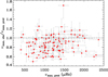 |
Fig. A.1. Ratio of the observed νmax, obs and the predicted νmax, pred using the spectroscopic log g. The dashed line shows the equality of both values. |
Appendix B: Candidates for solar-like oscillation detections
In this appendix, we present the results for the possible detections of solar-like oscillations in 26 targets. As explained in Section 3.2, these targets were not selected because the S/N was too low. In some cases, only one pipeline reported a detection and in other cases the location of the possible νmax was within 30% of the predicted value. These candidates do not have a reliable mean large frequency spacing but we report their approximative νmax in Table B.1. In Figure B.1, we show the comparison between the predicted νmax and the observed one similarly to Figure 4, where we used the surface gravities from B20. Like our sample with confirmed detections, the predicted frequency of maximum power seems to be overestimated but by a larger amount of 12.6% on average.
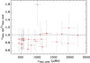 |
Fig. B.1. Ratio of the observed νmax, obs and the predicted νmax, pred using the log g from B20. Same details as in Figure 4 for the targets with possible detection of solar-like oscillations represented with red diamonds. |
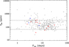 |
Fig. B.2. Magnetic activity proxy, Sph vs surface rotation period, Prot for the G14 sample (grey circles) and the targets with possible detection of solar-like oscillations and with detection of rotation modulation (squares). Same details as in Figure 11. |
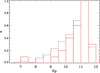 |
Fig. B.3. Normalized histogram of the Kepler magnitude for the C14 sample (black dashed line) and the targets with possible detection of solar-like oscillations (red solid line). |
Seismic and stellar parameters of the 26 candidates with possible seismic detections. Frequency of maximum oscillation power, νmax, is approximated. Same flags as in Table 1. The full table is available at the CDS.
During the visual checks, a few interesting cases were flagged. KIC 2578869 seems to show modes only below νmax, which is not something we have seen in the past and, thus, this star was put in the candidate list. KIC 11498538 has a strong rotation peak and the background would suggest that the modes are around 850 μHz, however, the modes are barely visible, probably due to the high level of activity of the star (e.g., Mathur et al. 2019; Gaulme et al. 2020). The last star that was flagged is KIC 11818430, which seems to present two signals in the échelle diagram and might be a binary star.
As for the confirmed sample, we searched for signature of rotation modulation in the light curves of these candidates. We find that 15 stars have a reliable Prot (see Table B.2), among which 3 stars are flagged as close binary candidates. The magnetic activity proxy values of the candidates are similar to the Sun from minimum to maximum magnetic activity (see Figure B.2).
Finally, the magnitude distribution of the candidates, shown in Figure B.3, is similar to the one for the C14 sample, peaking at a magnitude of 11.
Rotation periods and magnetic activity levels of the 15 stars with possible seismic detections.
Appendix C: Rotation analysis examples
We show here some examples of light curves of stars with measured rotation periods reported in this paper, along with the rotation analysis as described in Section 6.
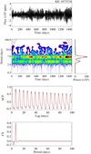 |
Fig. C.1. Surface rotation analysis of KIC 107775748. Top row: KEPSEISMIC light curve for KIC 10775748. Second row: Wavelet power spectrum (left), and global wavelet power spectrum (right; black), where the best fit with multiple Gaussian functions is shown in red. Third row: Autocorrelation function (ACF) of the light curve in black and its smoothed version in red. Bottom row: Composite spectrum (black) and best fit with multiple Gaussian functions (red). The dashed lines mark the rotation-period estimates from each diagnostic. |
Appendix D: Radii comparison with a different Teff scale
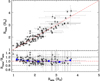 |
Fig. D.1. Comparison between the seismic radii after applying the Mosser et al. (2013) corrections on Δν and the Gaia radii (top panel) and ratio of the radii for our sample (bottom panel) but using the effective temperature from B20 in the seismic scaling relations to compute the radii, Rseis. Same details as in Figure 12. |
We computed the seismic radii using the effective temperatures from B20. The comparison with the B20 radii is shown in Figure D.1. The agreement is slightly better than when using the spectroscopic Teff.
Appendix E: Full table of global seismic parameters for the 624 solar-like stars
Global seismic parameters from A2Z for the 624 stars detection of solar-like oscillations. The full table is available at the CDS.
All Tables
Global seismic parameters from A2Z for the 525 stars with previous detection of solar-like oscillations.
Rotation periods and magnetic activity levels of the 63 stars with seismic detections.
Seismic and stellar parameters of the 26 candidates with possible seismic detections. Frequency of maximum oscillation power, νmax, is approximated. Same flags as in Table 1. The full table is available at the CDS.
Rotation periods and magnetic activity levels of the 15 stars with possible seismic detections.
Global seismic parameters from A2Z for the 624 stars detection of solar-like oscillations. The full table is available at the CDS.
All Figures
|
Fig. 1. Comparison of the Power Spectrum Density of KIC 4484238 using the DR24 data (black curve) and the DR25 data (red curve). |
| In the text | |
|
Fig. 2. Seismic Hertzsprung-Russell Diagram where the mean large frequency separation is used instead of the luminosity. The C14 solar-like stars are represented with grey circles where the effective temperature is taken from the M17. The 99 stars with confirmed seismic detections are shown with red squares where the effective temperature is coming from APOGEE, LAMOST or B20 (see Sect. 3.1). The position of the Sun is indicated by the ⊙ symbol and the grey solid lines represent evolution tracks from ASTEC (Christensen-Dalsgaard 2008) for a range of masses at solar composition (Z⊙ = 0.0246). Typical uncertainties are represented in the bottom left corner. |
| In the text | |
|
Fig. 3. Mean large frequency spacing, Δν, as a function of the frequency of maximum power, νmax for the C14 sample (grey circles) and our sample (red squares). Typical uncertainties are shown in the upper left corner. |
| In the text | |
|
Fig. 4. Ratio of the observed νmax, obs and the predicted νmax, pred using the log g from B20. The dashed line shows the equality of both values. |
| In the text | |
|
Fig. 5. Granulation frequency (top panel) and power (bottom panel) as a function of the frequency of maximum power. The stars in our sample are represented with red squares while the subsample of 163 stars from C14 are represented with grey circles. The blue dashed lines are the relations derived by Kallinger et al. (2014). |
| In the text | |
|
Fig. 6. Bolometric maximum amplitude of the modes as a function of νmax. The legend is the same as in Fig. 5. The blue dashed line corresponds to the fit for the stars from C14. |
| In the text | |
|
Fig. 7. Radius versus mass diagram for the C14 stars using S17 parameters (grey circles) and the stars in our sample described in this work (red diamonds). For the latter, corrections on Δν were applied following Mosser et al. (2013). |
| In the text | |
|
Fig. 8. Surface rotation periods, Prot, as a function of effective temperature, Teff, for the G14 sample (grey circles) and our sample (red squares). Typical error bars are shown in the bottom right corner. |
| In the text | |
|
Fig. 9. Normalized histogram of the Kepler magnitude for the C14 sample (black dashed line) and our sample (red solid line). |
| In the text | |
|
Fig. 10. Normalized histogram of the Kepler metallicity for the C14 sample (black dashed line) and for our sample (red solid line) for the 95 stars with new seismic detections and with APOGEE or LAMOST spectroscopic observations. |
| In the text | |
|
Fig. 11. Magnetic activity proxy, Sph vs surface rotation period, Prot for the G14 sample (grey circles) and our sample (squares). The blue square is the close binary candidate, KIC 4255487. The dashed lines correspond to the Sph values between minimum and maximum magnetic activity from Mathur et al. (2019). The typical error bars are represented in the bottom right-hand side. |
| In the text | |
|
Fig. 12. Left panel: comparison between the seismic radii after applying the Mosser et al. (2013) corrections on Δν and the Gaia radii (top panel) and ratio of the radii for our sample (bottom panel). The blue squares represent the median binned data. Only 97 stars are shown as two targets do not have a Gaia radius. Right panel: same details but for the S17 sample. |
| In the text | |
|
Fig. 13. Left panel: Differences between the Gaia radius and the seismic radius in units of the statistical uncertainty (σ), computed as the quadratic sum of the uncertainties from the B20 radii and the scaling relations radii. Right panel: histogram of the same differences. Dashed lines show the equality of both radii and the dot-dash lines represent the ±1σ limits. Only 97 stars are shown as two targets do not have a Gaia radius. The blue dashed line shows a Gaussian fit of the histogram. |
| In the text | |
|
Fig. A.1. Ratio of the observed νmax, obs and the predicted νmax, pred using the spectroscopic log g. The dashed line shows the equality of both values. |
| In the text | |
|
Fig. B.1. Ratio of the observed νmax, obs and the predicted νmax, pred using the log g from B20. Same details as in Figure 4 for the targets with possible detection of solar-like oscillations represented with red diamonds. |
| In the text | |
|
Fig. B.2. Magnetic activity proxy, Sph vs surface rotation period, Prot for the G14 sample (grey circles) and the targets with possible detection of solar-like oscillations and with detection of rotation modulation (squares). Same details as in Figure 11. |
| In the text | |
|
Fig. B.3. Normalized histogram of the Kepler magnitude for the C14 sample (black dashed line) and the targets with possible detection of solar-like oscillations (red solid line). |
| In the text | |
|
Fig. C.1. Surface rotation analysis of KIC 107775748. Top row: KEPSEISMIC light curve for KIC 10775748. Second row: Wavelet power spectrum (left), and global wavelet power spectrum (right; black), where the best fit with multiple Gaussian functions is shown in red. Third row: Autocorrelation function (ACF) of the light curve in black and its smoothed version in red. Bottom row: Composite spectrum (black) and best fit with multiple Gaussian functions (red). The dashed lines mark the rotation-period estimates from each diagnostic. |
| In the text | |
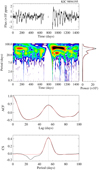 |
Fig. C.2. Surface rotation analysis of KIC 9894195. Same as Figure C.1 for KIC 9894195. |
| In the text | |
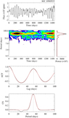 |
Fig. C.3. Surface rotation analysis of KIC 10969935. Same as Figure C.1 for KIC 10969935. |
| In the text | |
|
Fig. D.1. Comparison between the seismic radii after applying the Mosser et al. (2013) corrections on Δν and the Gaia radii (top panel) and ratio of the radii for our sample (bottom panel) but using the effective temperature from B20 in the seismic scaling relations to compute the radii, Rseis. Same details as in Figure 12. |
| In the text | |
Current usage metrics show cumulative count of Article Views (full-text article views including HTML views, PDF and ePub downloads, according to the available data) and Abstracts Views on Vision4Press platform.
Data correspond to usage on the plateform after 2015. The current usage metrics is available 48-96 hours after online publication and is updated daily on week days.
Initial download of the metrics may take a while.