| Issue |
A&A
Volume 674, June 2023
|
|
|---|---|---|
| Article Number | A106 | |
| Number of page(s) | 25 | |
| Section | Stellar structure and evolution | |
| DOI | https://doi.org/10.1051/0004-6361/202244577 | |
| Published online | 09 June 2023 | |
Multi-campaign asteroseismic analysis of eight solar-like pulsating stars observed by the K2 mission
1
Instituto de Astrofísica de Canarias (IAC), Vía Láctea s/n, La Laguna, 38200 Tenerife, Spain
e-mail: luciagc@iac.es
2
Departamento de Astrofísica, Universidad de la Laguna, La Laguna, 38200 Tenerife, Spain
3
Université Paris-Saclay, Université Paris Cité, CEA, CNRS, AIM, 91191 Gif-sur-Yvette, France
4
École CentraleSupélec, Université Paris-Saclay, 91190 Gif-sur-Yvette, France
5
Bay Area Environmental Research Institute, PO Box 25 Moffett Field, CA, 94035
USA
6
NASA Ames Research Center, Moffett Field, CA, 94035
USA
Received:
22
July
2022
Accepted:
26
February
2023
The NASA K2 mission that succeeded the nominal Kepler mission observed several hundred thousand stars during its operations. While most of the stars were observed in single campaigns of ∼80 days, some of them were targeted for more than one campaign. We perform an asteroseismic study of a sample of eight solar-like stars observed during K2 Campaigns 6 and 17, allowing us access to up to 160 days of data. With these two observing campaigns, we determine not only the stellar parameters but also study the rotation and magnetic activity of these stars. We first extract the light curves for the two campaigns using two different pipelines, EVEREST and Lightkurve. The seismic analysis is done on the combined light curve of C6 and C17, where the gap between them was removed and the two campaigns were ‘stitched’ together. We determine the global seismic parameters of the solar-like oscillations using two different methods: one using the A2Z pipeline and the other the Bayesian apollinaire code. With the latter, we also perform the peak-bagging of the modes to characterize their individual frequencies. By combining the frequencies with the Gaia DR2 effective temperature and luminosity, and metallicity for five of the targets, we determine the fundamental parameters of the targets using the IACgrids based on the MESA (Modules for Experiments in Stellar Astrophysics) code. We find that four of the stars are on the main sequence, two stars are about to leave it, and two stars are more evolved (a subgiant and an early red giant). While the masses and radii of our targets probe a similar parameter space compared to the Kepler solar-like stars, with detailed modeling, we find that for a given mass our more evolved stars seem to be older than previous seismic stellar ensembles. We calculate the stellar parameters using two different grids of models, one incorporating and one excluding the treatment of diffusion, and find that the results agree generally within the uncertainties, except for the ages. The ages obtained using the models that exclude diffusion are older, with differences of greater than 10% for most stars. The seismic radii and the Gaia DR2 radii present an average difference of 4% with a dispersion of 5%. Although the agreement is relatively good, the seismic radii are slightly underestimated compared to Gaia DR2 for our stars, the disagreement being greater for the more evolved ones. Our rotation analysis provides two candidates for potential rotation periods but longer observations are required to confirm them.
Key words: asteroseismology / stars: activity / stars: fundamental parameters / stars: oscillations
© The Authors 2023
 Open Access article, published by EDP Sciences, under the terms of the Creative Commons Attribution License (https://creativecommons.org/licenses/by/4.0), which permits unrestricted use, distribution, and reproduction in any medium, provided the original work is properly cited.
This article is published in open access under the Subscribe to Open model. Subscribe to A&A to support open access publication.
1. Introduction
Thanks to data collected by missions such as CoRoT (Convection, Rotation, and Transits, Baglin et al. 2006) and Kepler/K2 (Borucki et al. 2010; Howell et al. 2014), asteroseismology has been shown to be a powerful tool for determining more precise stellar parameters compared to classical methods and provides information on stellar interiors (e.g., Aerts 2021).
For stars like the Sun, with an internal radiative zone and a convective envelope, solar-like oscillations are generated by the turbulent motions in the outer layers of the star, yielding stochastically excited modes. The excellent precision of the Kepler observations led to many asteroseismic studies of stars with gravito-acoustic oscillations. Indeed, solar-like oscillations have been detected and characterized in hundreds of stars on the main sequence and on the subgiant branch (e.g., García et al. 2009; Serenelli et al. 2017; García & Ballot 2019; Jackiewicz 2021) as well as in tens of thousands of red giants (e.g., Yu et al. 2018). In addition, several tens of planet-host stars have been characterized with asteroseismology, enabling a more precise measurement of the radii and ages of the planets (e.g., Huber et al. 2013; Campante et al. 2015; Silva Aguirre et al. 2015).
The NASA Kepler Mission ended in May 2013 because of a failure on the second of the four reaction wheels of the satellite. This problem made it impossible to continue with the nominal mission and the situation forced the team to design a new observation strategy, giving rise to the K2 mission (Howell et al. 2014). This mission resulted in 20 observation campaigns of around 80 days along the ecliptic plane in different regions of the Galaxy. In the early campaigns of the K2 mission, solar-like oscillations were detected in 36 solar-like stars including 3 planet-host stars (Chaplin et al. 2015; Lund et al. 2016, 2019; Van Eylen et al. 2018; Smith et al. 2022) as well as in several tens of thousands of red giants (Stello et al. 2017; Zinn et al. 2020, 2022).
There are some overlapping campaigns1, which enable us to double the observation time for several targets. This is the case for campaigns C6 and C17, yielding a sample of 12 solar-like stars that have been observed in both campaigns in short cadence. Among them, solar-type oscillations have been detected with a sufficiently high signal-to-noise ratio for asteroseismic analysis for eight stars2 and with a Gaia renormalized unit weight error (RUWE) value below 1.25 to avoid possible binaries. These are the stars we analyze in this study with asteroseismology. We note that five of our targets (EPIC 212478598, EPIC 212485100, EPIC 212487676, EPIC 212516207 and EPIC 212683142) have also been seismically studied by Ong et al. (2021), but these authors only analyzed one campaign (C6). Our work uses time series of twice the length of the C6 campaign, and therefore we achieve a higher resolution compared to this latter analysis, and we show in Sect. 4.2 that we retrieve more modes at higher and lower frequency, as well as higher degree modes. In addition, we present a new asteroseismic analysis for further three solar-like stars (EPIC 212509747, EPIC 212617037 and EPIC 212772187).
We note that two other stars show solar-like oscillations in both campaigns. EPIC 212708252 is a solar analog with a RUWE value of 1.274, which is slightly above our cut. This latter star is part of another study devoted to solar analogs (García et al., in prep.). EPIC 212709737 is a hot F dwarf with a Gaia effective temperature of around 6500 K, and the modes are wide, as expected for such a hot star (Appourchaux et al. 2012a), making their characterization more complicated. In addition, with a RUWE value of 2.469, it is more likely to be in a binary system. This star is currently under spectroscopic follow up, and a longer time line is required for a full analysis of the system, which is out of the scope of this paper.
The layout of the paper is as follows: in Sect. 2, we describe the data we used and the procedure to calibrate the light curves for our asteroseismic analyses. In Sect. 3, we describe the atmospheric parameters of our sample of stars, and in Sect. 4, we explain how we use these parameters to model the stars and the procedure followed to characterize the modes. In Sect. 5, we discuss the results from the stellar modeling, as well as the analysis of the rotation and magnetic activity of the stars. Finally, in Sect. 6, we provide the conclusions of this work.
2. Photometric observations
We select eight stars observed in short-cadence (SC; dt ∼ 1 min; see Gilliland et al. 2010, for more details) mode in both campaigns, C6 and C17, for which signatures of a p-mode hump were found. The full list of stars, which we refer to with the letters A to H, is shown in Table 1 along with their general properties.
Atmospheric and global seismic parameters for our sample of stars with their corresponding letter references from A to H.
Compared to the nominal Kepler mission, the K2 observations suffer additional systematic uncertainties due to the scheme adopted to stabilize the satellite with only two working reaction wheels. Increased spacecraft roll motion around the boresight caused a saw-tooth-shaped systematic error in the mission light curves on timescales of approximately 6 h. Several pipelines have been developed to produce light curves without these systematic errors and properly calibrate the K2 data (e.g., Vanderburg & Johnson 2014; Lund et al. 2015; Aigrain et al. 2016; Luger et al. 2016). For this work, we used two of those pipelines. The first is the EVEREST3 (Ecliptic Plane Input Catalog Variability Extraction and Removal for Exoplanet Science Targets) pipeline (Luger et al. 2016, 2018) that has been shown to provide calibrated data that are well suited to asteroseismic analyses of red giants (e.g., White et al. 2017; Zinn et al. 2020, 2022). However, for the short-cadence data, only light curves up to C13 are available with this calibration. Hence, we also used an adapted version of the Lightkurve Python package4 (Lightkurve Collaboration 2018) to generate the short-cadence light curves for C17.
We first extracted the Target Pixel File (TPF) downloaded from the Mikulski Archive for Space Telescopes (MAST). We created a customized aperture for asteroseismic analyses where we took pixels with an average flux of greater than 1.4 × 10⁵ e− s−1. Figure 1 shows our customized mask compared to the raw TPF and the pipeline mask for HD 115680 (A). We then applied the self-flat-fielding corrector (Zhang et al. 2018), which takes into account the timescale of the filter as well as the number of segments in which the 6 h correction is done. By comparing the power spectral densities (PSD) of the eight stars observed in C6 with both pipelines, we minimized the differences by tweaking the different parameters of the filter. The best results were obtained using ten segments for the window keyword and a timescale of 1 day.
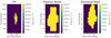 |
Fig. 1. Comparison of the standard K2 aperture (left panel), the standard Lightkurve pipeline mask (middle panel), and our customized mask (right panel), taking pixels with an average flux larger than 1.4 × 10⁵ e− s−1 for HD 115680 (A). |
Using these two calibration methods, we denote the outputs as C6EV from EVEREST, and C6LK and C17LK from Lightkurve. A comparison of the PSDs of HD 115427 (D) is given in Appendix A. In general, EVEREST light curves have lower noise than those from Lightkurve. To increase the frequency resolution of the spectrum compared to the study of a single, isolated campaign, and improve the overall signal-to-noise ratio (S/N) of the PSD while obtaining the longest time series with which to study the oscillation modes and the surface rotation and magnetism, we “stitch” the data of both campaigns together, removing the gap between them. To do so, the first point of C17 is placed just one cadence after the last point of C6. Because these are solar-like pulsating stars with incoherent modes, the effect of removing the ∼2.5 year gap only slightly modifies the widths of the modes that have lifetimes longer than the gap (for more details see Ballot et al. 2004a,b). The longest living p modes in the stars analyzed in this work have lifetimes of around 3.7 days. Therefore, during the 2.5 year gap, all the modes are re-excited hundreds of times and there is therefore no effect in the characterization of the central frequencies of the limit spectrum. A detailed Monte Carlo simulation of the long-lived modes in EPIC 212485100 is described in Appendix B, where we justify this choice.
As C17LK is noisier than C6EV, we apply a correction factor to scale the two campaigns on a similar level. To do so, we multiply the C17LK flux by the ratio of the noise in the PSDs above 6 mHz between C6 and C17, as follows:
where the symbol < > indicates the mean of the PSD.
Light curves from both EVEREST and Lightkurve are then processed with the Kepler Asteroseismic Data Analysis Correction Software pipeline (KADACS, García et al. 2011). Gaps shorter than 5 days are filled with inpainting techniques using a multi-scale discrete cosine transform (García et al. 2014a; Pires et al. 2015) following what has been applied to Kepler data. The light curves produced in this work are available at gitlab5.
3. Atmospheric parameters
We consolidated the atmospheric parameters (effective temperature and surface gravity), as well as luminosity, from the literature in order to use them as inputs in the stellar modeling. The most comprehensive catalog for the K2 targets is the Ecliptic Plane Input Catalog (EPIC, Huber et al. 2016), which classified around 138 000 K2 targets, providing in particular effective temperature (Teff), surface gravity (log g), and metallicity ([Fe/H]) for the K2 stars. Those parameters were inferred from colors, parallaxes, and spectroscopic information when available and the stellar population synthesis model Galaxia (Sharma et al. 2011). However, since the delivery of EPIC, observations from the Gaia mission (Perryman et al. 2005) have provided improved and more precise parallaxes with the Data Release 2 (Gaia Collaboration 2018). We therefore took the DR2 effective temperature and luminosity derived by the Gaia team. We note that, as this work was nearing completion, Gaia DR3 became available. Some of our targets have spectroscopic parameters in the GSP-Spec module (Recio-Blanco et al. 2023), but a comparison with the DR2 parameters showed that the Teff and log g values agree within 1 and 2σ, respectively. For metallicity, while GSP-Spec values are available for our targets, we did not use them because of their very small error bars, as well as the potential systematic errors in the metallicity scale when compared to other surveys (Gaia Collaboration 2023). For five of our targets, Ong et al. (2021) obtained high-resolution spectra, providing Teff and [Fe/H]. Their effective temperatures agree with the Gaia DR2 values within 2σ, and so we kept the Gaia constraints, while we used the metallicity from Ong et al. (2021). For the remaining three stars, we decided to carry out our analysis using the parameters from Gaia DR2, which do not include metallicity values (but see Sect. 4 for a comparison of the results had we used Gaia DR3 instead). The consolidated atmospheric parameters and Gaia luminosity of our eight targets are given in Table 1.
4. Seismic analysis
Our targets were observed for ∼160 days when combining the two campaigns. We first estimated the global seismic parameters and then characterized the individual modes.
4.1. Global seismic parameters
Asteroseismology is the study of the internal structure and dynamics of the stars by means of their resonant oscillations (e.g., Turck-Chièze et al. 1993; Christensen-Dalsgaard 2002). These vibrations manifest themselves as small motions of the visible surface of the star and as associated small variations of stellar luminosity.
In this work, we study the acoustic (p) modes that are produced in the interior of solar-like stars from the turbulence in their outer layers. P modes of the same degree ℓ are asymptotically equidistant in frequency (Tassoul 1980), which allows us to define some global parameters of the p-mode pattern that we define below.
The first of these global parameters is the frequency of maximum mode power, νmax. This is the frequency of the maximum of the power envelope of the oscillations (usually fitted by a Gaussian function), where the observed modes present their strongest amplitudes. This parameter can be related to the cut-off frequency in the stellar atmosphere and therefore to the stellar surface gravity and the effective temperature of the star (Brown et al. 1991; Belkacem et al. 2011).
The second global seismic parameter is the large frequency spacing, Δν. This is the average spacing in frequency between consecutive radial-order modes of the same angular degree and is directly proportional to the mean density of the star (Kjeldsen & Bedding 1995). We determined these two fundamental quantities with two different methods.
4.1.1. A2Z pipeline
We performed the first analysis of global seismic parameters with the A2Z pipeline (Mathur et al. 2010), where the mean large frequency spacing is computed by considering the power spectrum of the PSD itself. The frequency of maximum power is obtained from fitting a Gaussian on the p-mode bump after having subtracted the background fit on the PSD. The background model consists of three components: two Harvey functions (Harvey et al. 1985) to model different scales of convection and a constant representing the photon noise. Each Harvey function is as follows:
where A is the reduced-amplitude component, νc is the characteristic frequency, and γ is the exponent of the Harvey model, which we fixed to a value of 4 (e.g., Kallinger et al. 2014). We note that for the background fit, we only took into account the PSD above 200 μHz for all the stars in our sample because of the instrumental trends at lower frequencies.
4.1.2. apollinaire pipeline
The second method that we applied is the Bayesian Python module apollinaire6 from Breton et al. (2022). Through the implementation of the emcee Ensemble sampler (Foreman-Mackey et al. 2013), the module implements Markov chain Monte Carlo (MCMC) sampling of the parameter posterior probability distribution of background and p-mode models. Following an approach similar to those presented in Mosser et al. (2011a), Lund et al. (2017), Corsaro et al. (2020), and Nielsen et al. (2021) for example, the p-mode profile can be fitted with a global parametrization or by considering individual mode parameters as explained in Sect. 4.2.
The apollinaire pipeline starts fitting the background based on a model similar to that of the A2Z pipeline. This model is based on two Harvey functions (Harvey et al. 1985) with an exponent also fixed to 4, a Gaussian function for the bump of the p modes, and the photon noise. The fit was carried out with 1000 steps (including 500 steps for the initial burn-in phase) and 500 walkers, starting at a frequency of 50 μHz.
We then fit the asymptotic relation of the p modes based on the Tassoul (1980) development, where the frequency of a mode is described as:
where the order n is much larger than the degree ℓ in this approximation and ϵ is a phase offset. The relation used in apollinaire follows the suggestion of Lund et al. (2017) and extends this relation to the second order:

where δν0ℓ corresponds to the small separations between the modes of degree 0 and the mode of degree ℓ (see Breton et al. 2022, for more details). α and β0ℓ are the curvature terms on Δν and δν0ℓ, respectively. Finally, nmax is given by
The description given above is best for main sequence stars. However, for more evolved stars, such as subgiants, the presence of mixed modes makes the pattern less regular and a different approach has to be followed. Mixed modes propagate as pressure waves in the convective envelope and as gravity waves in the radiative interior; they typically reach the stellar surface with amplitudes larger than g modes (e.g., Beck et al. 2011; Bedding et al. 2011; Mosser et al. 2011b). Therefore, as long as they have enough amplitude at the surface to be detectable, they can be used to probe the inner radiative core with high precision. Unfortunately, deriving the central frequencies of these modes is not straightforward with an asymptotic formulation (e.g., Appourchaux 2020). To avoid any perturbation of these mixed modes in apollinaire’s universal pattern fit, the regions of the PSD around these modes are removed and noise is added to have a continuous level between the remaining pairs of modes ℓ = 0, 2. A detailed description of the procedure to follow can be found in Appendix B of Breton et al. (2022).
An important parameter of the mode-pattern fit is the phase offset ϵ, as it allows us to determine whether the identification of the mode degree is correct. This is particularly useful for stars with low S/N. To confirm the correct identification, we used the ϵ − Teff diagram as shown by White et al. (2012). ϵ can be calculated from the fitted frequencies of the ℓ = 0 and the value of Teff by Eq. (3). If the extracted value does not fit the general trend of the ϵ − Teff relation, the identification is wrong. In that case, we re-run the universal pattern fit changing the guess in the ϵ value given as input.
4.1.3. Global seismic parameters with A2Z and apollinaire
We ran both codes on the EVEREST calibrated light curves (C6), the Lightkurve data (C6 and C17), and on the stitched C6 and C17 (C6+C17) time series. We compared the results obtained from the two pipelines for the different observing campaigns (C6EV, C6LK, C17LK) as well as for the combined campaigns (C6+C17), finding that for all the analyzed light curves, the values of Δν and νmax obtained with A2Z and apollinaire agree within 3σ, and within 1σ between C6EV and C6+C17.
In addition we compared the absolute uncertainties provided by each method. The error bars on νmax are generally smaller for A2Z by up to a factor of 2, while for Δν, the uncertainties are significantly smaller for apollinaire by a factor of 5 to 6.
Given the results of the comparison between the two pipelines, and for compatibility with previous published values of A2Z for other stars, we decided to use the A2Z global seismic parameters obtained with the combined C6+C17 calibrated light curves for the stellar modeling. We also remind the reader that Δν values obtained by the A2Z pipeline are “global” compared to apollinaire, which performs the universal pattern fit using only five orders around νmax, an approach usually referred to as “local” (Christensen-Dalsgaard et al. 2014), which can explain these small differences.
The results obtained for νmax are combined with Teff from Gaia DR2 to estimate the seismic log g using the following equation:
where νmax, ⊙ = 3090 ± 30 μHz, Teff, ⊙ = 5777 K7, and g⊙ = 27 402 cm s−2 (Brown et al. 1991; Kjeldsen & Bedding 1995). Global seismic parameters and surface gravities are given for all the stars in Table 1.
4.2. Peak bagging
Individual p and mixed modes of all the stars were obtained with the fitting module of apollinaire using 500 walkers and 5500 steps (including a burn-in phase of 500). From the universal pattern fit described above, initial guesses of p modes in a range of seven orders around νmax were automatically created by the code. By visually inspecting these guesses, we can modify those parameters that appear to be incorrect and perform a first fitting. Then, we divide the PSD by the initial fitted model to obtain a residual PSD in S/N and all peaks lying where a mode is expected and with a S/N above 8 are added to the guesses and the fit is repeated. Finally, for the two subgiant stars, we carry out a final fit including the mixed-mode candidates. To do so, we select all peaks with a high S/N that were not identified as ℓ = 0, 2, or 3 modes and we fit them assuming that they could be potential mixed modes. The tables with the resulting frequencies for all the stars are given in Appendix C and the échelle diagrams are given in Appendix D.
For the five stars of our sample also analyzed by Ong et al. (2021), the additional modes that we fitted in our work are flagged in the tables of mode frequencies in Appendix C. As expected with the longer time series used in this work, we find that, on average, with our analysis we fit a couple of additional orders at high frequency and one additional order at low frequency as well as higher degree modes (ℓ = 2 or 3). We also provide a comparison of the fitted frequencies of the five stars in Appendix E. We find that the frequencies of the common modes between the two analyses agree within 4σ.
4.3. Stellar modeling
Model fitting is based on a set of grids of stellar models. The main grid consists of models evolved from the pre-main sequence to the red giant branch (RGB) using the MESA code (Modules for Experiments in Stellar Astrophysics; Paxton et al. 2011, 2013, 2015), version 15 140. The OPAL opacities (Iglesias & Rogers 1996) and the GS98 metallicity mixture (Grevesse & Sauval 1998) were used; otherwise the standard input physics from MESA was applied. This main grid is composed of evolutionary sequences with masses M from 0.8 M⊙ to 1.5 M⊙ with a step of ΔM = 0.01 M⊙, initial abundances [M/H] from −0.3 to 0.4 with a step of 0.05, and mixing length parameters α from 1.5 to 2.2 with a step of Δα = 0.05. The mixing length theory is modeled according to Cox & Giuli (1968). Eigenfrequencies were computed in the adiabatic approximation using the ADIPLS code Christensen-Dalsgaard (2008a).
A second grid of models was built with the same range of parameters but including microscopic diffusion. A third grid includes diffusion and overshooting, implemented with the exponential prescription given by Herwig (2000). This grid was limited to masses of between 1.3 M⊙ and 1.39 M⊙ and the overshooting parameter was fixed to f = 0.02, which is a standard value in this description (see Pérez Hernández et al. 2019, for a quick reference to the equation).
The initial metallicity Z and helium abundance Y were derived from [M/H], and were constrained by taking a Galactic chemical evolution model with ΔY/ΔZ = (Y⊙ − Y0)/Z⊙ fixed. Assuming a primordial helium abundance of Y0 = 0.249 and initial solar values of Y⊙ = 0.2744 and Z⊙ = 0.0191 (consistent with the opacities and GS98 abundances considered above), a value of ΔY/ΔZ = 1.33 is obtained. A surface solar metallicity of (Z/X)⊙ = 0.0229 was used to derive values of Z and Y from the [M/H] interval. Hereafter, we refer to this set of model grids as IACgrid.
For a typical evolutionary sequence in the initial grid, we save about 100 models from the zero age main sequence (ZAMS) to the terminal age main sequence (TAMS). Owing to the very rapid change in the dynamical timescale of the models, tdyn = (R3/GM)1/2, such a grid is too coarse in the time steps. Nevertheless, the dimensionless frequencies of p modes change so slowly that interpolations between models introduce much smaller errors than the observational ones. This procedure was discussed in more detail in Pérez Hernández et al. (2016) and was found to be safe and to consume relatively little time.
The stellar parameters are found through a χ2 minimization that compares observed values to the grid of models discussed above. The general procedure is similar to that described in Pérez Hernández et al. (2019). Specifically, we minimize the function

Here, we define:
![$$ \begin{aligned} \chi ^2_{\mathrm{spec} } = \frac{1}{3} \left[\left(\frac{\delta T_{\rm eff}}{\sigma _{T_{\rm eff}}}\right)^2 + \left(\frac{\delta g}{\sigma _{g}}\right)^2 + \left(\frac{\delta (Z/X)}{\sigma _{ZX}}\right)^2 + \left(\frac{\delta L}{\sigma _{L}}\right)^2\right], \end{aligned} $$](/articles/aa/full_html/2023/06/aa44577-22/aa44577-22-eq8.gif)
where δTeff, δg, δ(Z/X), and δL correspond to differences between the observations and the models whereas σTeff, σg, σZ/X, and σL are their respective observational errors. Values for L, Teff, and their errors are given in Table 1 but log g was derived from νmax and Teff using the seismic scaling relation (see Eq. (6)). Here, we assumed a systematic error of 0.1 dex for the main sequence stars and 0.2 dex for the RGB stars. Finally, as mentioned before, values of Z/X where taken from Ong et al. (2021) when available.
The term  in Eq. (7) corresponds to the frequency differences between the models and the observations after removing a smooth function of frequency in order to filter out surface effects not considered in the modeling. This surface term is computed only using radial oscillations as described in Pérez Hernández et al. (2019). When the surface term is determined, we consider radial as well as nonradial modes for computing the corresponding minimization function
  . Finally,
  takes into account the dynamical time. For more information on the χ2, we refer to Pérez Hernández et al. (2016, 2019).
To estimate the uncertainty in the output parameters, we assumed normally distributed uncertainties for the observed frequencies, mean density, and spectroscopic parameters. We then searched for the model with the minimum χ2 in every realization and computed mean values and standard deviations.
5. Discussion
5.1. Comparison between the observed and predicted frequency of maximum power
The seismic scaling relation given in Eq. (6) can be inverted to calculate an estimation of the frequency of maximum power if we have the effective temperature and the surface gravity of a star. Therefore, thanks to the EPIC, we obtain a first estimation of the global seismic parameters.
A second estimation of νmax can be calculated using the effective temperatures and radii from the Gaia DR2 stellar parameters catalog (Andrae et al. 2018) using Eq. (9):
where νmax, ⊙ = 3090 ± 30 μHz, Teff, ⊙ = 5777 K, and R⊙ = 6.957e + 10 cm (Chaplin & Miglio 2013; Belkacem et al. 2013).
Figure 2 shows the comparison between the observed νmax and the expected values from EPIC and Gaia stellar parameters. We can see some difference between the two catalogs. Indeed, the effective temperatures are in many cases very different between the EPIC and Gaia. As expected, estimations of νmax using data from Gaia DR2 are more consistent with the seismic observations than those obtained from the EPIC data, as for the majority of the stars they agree within 1σ. This suggests that the precision of the Gaia DR2 parameters is enough to predict the frequency region of the p modes for our sample of solar-like stars.
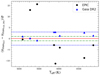 |
Fig. 2. Ratio of the difference between the observed νmax and the estimation from EPIC data (black circles) and Gaia DR2 data (blue triangles), and the combined uncertainties, σ. The green dot-dashed lines correspond to ±1σ and the blue dashed lines represent the 3σ limits, where sigma is the square root of the sum of the quadratic errors. The red continuous line depicts the null difference. |
5.2. Stellar parameters from asteroseismology
Using Teff, L, and νmax combined with the individual frequencies of the p modes, we looked for the best-fit models of our eight targets with the IACgrid described in Sect. 4.3. The main stellar parameters from the best-fit model are obtained with the grid without treatment of diffusion. They are listed in Table 2. We also list the results coming from the grid that includes diffusion, which allows us to gauge the effect of different physics in the models. We return to this point later.
Stellar parameters from the seismic modeling.
In Fig. 3, we show the location of our targets in a modified seismic Hertzsprung-Russell diagram (HRD) along with the 624 Kepler solar-like stars with a detection of p modes (Mathur et al. 2022). Our sample of stars is in general more massive than the Sun (above 1.2 M⊙). We can also see the two evolved stars: one subgiant (HD 119026 (G)) and one early red giant (HD 115680 (A)). In addition, we note that from the best-fit models, two stars HD 114558 (C) and HD 117779 (F) are close to the terminal age main sequence (TAMS).
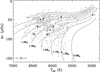 |
Fig. 3. Seismic Hertzsprung-Russell diagram, where the luminosity is modified by the mean large frequency spacing, Δν. The colored symbols represent the stars studied here: red triangles are the main sequence stars; blue stars are stars near the TAMS; orange squares are subgiants. The Kepler sample with detected solar-like oscillations (Mathur et al. 2022) are also represented with gray circles. The evolutionary tracks with solar metallicity from the Aarhus STellar Evolution Code (Christensen-Dalsgaard 2008a) are represented with the black lines. The average uncertainties on Teff and Δν are shown in the lower left corner. |
In the last column of Table 2, we list the χ2 values for the best-fit models. In general, all well-determined modes were used in the fit, but if this implied values χ2 > 3 then mixed ℓ = 1 modes were not considered. In general, this happens for the subgiants. Our IACgrid has only four free parameters: mass, metallicity, mixing length parameter, and age, while we are fitting four observed parameters and the individual mode frequencies. Furthermore, the frequency corrections considered to take into account surface uncertainties include mode inertia but not effects of the coupling between ℓ = 1 mixed modes. Although mixed modes can be very useful for probing the physics of the stellar interior, providing stellar parameters (such as age) with smaller uncertainties, the inclusion of these modes will yield results that are more model dependent than the ones reported here.
To better illustrate the fit of the observed frequencies, in Appendix D we show échelle diagrams of the eight stars with the comparison between the model frequencies with diffusion and the observed ones. Looking at the échelle diagrams in Appendix D, we also note that HD 119038 (H) and HD 115427 (D) have lower S/N compared to the other stars.
For HD 117779 (F), the Gaia data provide large error bars on both the luminosity (five times larger than for the other stars) and the effective temperature (250 K). The luminosity value also seems to be relatively high given the seismic parameters, which makes it more dubious. The fit without the luminosity constraint leads to a lower χ2 value (going from 2.1 to 1.1). We can also see in the échelle diagram that the ridges are not particularly clear. Being an evolved F-dwarf, the width of the modes is larger, which could lead to some confusion in the identification of the modes. Comparing the fitted frequencies to the model frequencies, the dipolar modes with n = 12 and 13 were not used for the modeling, because at this frequency range, the presence of mixed modes in the models ‘bumps’ the p-dominated modes and we are not able to stabilize the minimization when those modes are used.
As mentioned above, the identification of the modes can be done with the phase offset ϵ in Eq. (3). From the universal pattern of apollinaire, we therefore obtained an estimation for that parameter and represent it in the ϵ − Teff diagram (see Fig. 4). For comparison, we also added a sample of 119 Kepler solar-like stars where the frequencies of the individual modes were obtained by Appourchaux et al. (2012b), Davies et al. (2016), and Lund et al. (2017; gray circles). We can see the correlation between the two parameters: as the effective temperature increases, the ϵ value decreases. This emphasizes that the identification of the individual frequencies of our eight targets is the correct one. The early red giant, HD 115680 (A), is the coolest star in this diagram, sitting to the left hand side.
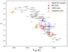 |
Fig. 4. Phase offset from the universal pattern fit of apollinaire, ϵ, as a function of Teff from Gaia DR2. The Kepler targets with characterized individual modes are represented with gray circles. MS stars in our sample, the two TAMS stars and the two subgiants are represented with red triangles, blue stars and orange squares, respectively. |
In Fig. 5, we compare the stellar parameters of our sample with the Kepler solar-like stars with detailed modeling from Silva Aguirre et al. (2015, 2017), represented with gray dots, and the subgiant sample modeled by Li et al. (2020) with dark gray squares. The mass as a function of the radius is shown in the upper left panel. The top right panel represents the mass as a function age and, finally, in the bottom panel, we show the age as a function of radius.
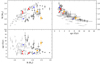 |
Fig. 5. Stellar fundamental parameters obtained with models without diffusion for our K2 targets (referred to with letters A through H) showing mass vs radius (upper left panel), mass vs age (upper right panel), and age vs radius (lower left panel). In all panels, main sequence stars are represented by red triangles, stars close to the TAMS with blue stars, and subgiant/red giant stars with orange diamonds. For comparison, Kepler solar-like stars with detailed seismic modeling are represented with gray circles (Silva Aguirre et al. 2015, 2017), while subgiants are shown with dark gray squares (Li et al. 2020). |
While the main sequence stars populate the same region of the M–R diagram, the more evolved stars move towards larger radii, as expected by stellar evolution. The two stars close to the TAMS (HD 114558 (C) and HD 117779 (F)) fall in the less populated region between the main sequence and subgiant stars.
It is also interesting to note that an evolved 1 M⊙ is in our sample, and falls in a relatively unpopulated region of the diagram. This is the early red giant in our sample, HD 115680 (A) star, with a radius of 2.47 ± 0.06 R⊙.
The top right panel of Fig. 5 also shows that, for a given mass, the evolved stars from our sample are among the oldest already known from the Kepler main-mission sample. We note that, in general, the changes in the stellar parameters when including diffusion are inside the internal uncertainties, except for the ages. Indeed, microscopic diffusion impacts the abundance of chemical elements inside the stars as they can migrate from the surface to the interior. As a consequence, the amount of H in the core can change and this can modify the stellar age (Fig. 6). Models without diffusion are older than models with diffusion. In the bottom panel of Fig. 6, we can see that the differences between the ages are larger than 10% in most of the stars. The mean internal error on the ages of 8% is clearly underestimating the systematic uncertainty in most cases.
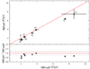 |
Fig. 6. Ages obtained with the IACgrid with diffusion vs ages from the IACgrid without diffusion (top panel). The one-to-one line is represented with the red dashed line. Ratio between the two different age computations as a function of the age from the IACgrid without diffusion (bottom panel). The red dashed line is the equality line while the gray dot-dashed lines correspond to the mean age uncertainty on stellar ages without diffusion of our sample (of 8%). |
For one star, HD 119038 (H), with a mass M ≃ 1.3 M⊙, we consider a fit to a grid of models with overshooting, as indicated in Sect. 4.3. As can be seen in Table 2, stellar parameters from the grid with overshooting are consistent with those derived from the grid without including it.
Finally, we compute results considering Teff and log g from the Gaia DR3 database as mentioned in Sect. 3. The ages, masses, and radii change on average by 13%, 6%, and 3%, respectively. These figures are slightly higher than the statistical errors given in Table 1. As mentioned previously, these results should be taken with caution because the spectroscopic values of log g in DR3 require further analysis.
5.3. Comparison between Gaia DR2 and seismic radii
The Gaia mission has provided radii for a large number of stars in our galaxy, including our eight targets. We decided here to compare the Gaia radii with the seismic ones. However, because we used the luminosity as an input in the models, the seismic analysis is clearly biased towards the Gaia radii. For an independent comparison, we also computed the best-fit models without the luminosity constraint. The result of the comparison is shown in Fig. 7. The agreement between Gaia and asteroseismic radii is, in general, relatively good for all the targets, except for HD 117779 (F), which is 1.5σ away. As mentioned above, this star has a large uncertainty on the luminosity and effective temperature as well as a low S/N in the PSD, making the identification of the modes more complicated. As a consequence, the seismic analysis of that star should be taken with caution.
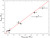 |
Fig. 7. Comparison between Gaia DR2 radii and radii from seismic modeling without using the luminosity constraint from Gaia for our eight targets. The red dashed line represents the one-to-one line. |
On average, we find that the difference between the seismic and Gaia radii is of 4% with a scatter of 5%. The seismic radii are slightly underestimated. However, the disagreement is larger for more evolved stars in the subgiant phase. This agrees with the previous comparisons between Gaia and asteroseismology carried out for hundreds of solar-like stars observed by the Kepler mission (e.g., Huber et al. 2017; Zinn et al. 2019; Mathur et al. 2022).
5.4. Study of the surface rotation
Stellar rotation periods are useful not only for the study of angular momentum transport in stars (Spada & Lanzafame 2020) but also to infer stellar ages via gyrochronology (Barnes 2007) given that stars on the main sequence were shown to spin down based on spectroscopic observations of young clusters (Skumanich 1972). Rotation periods obtained from asteroseismology or modulations in the light curve related to the presence of active regions and/or faculae at the surface of the star were combined with seismic ages, which led to the finding that some stars rotate faster, which is expected based on classical gyrochronology relations (Angus et al. 2015; van Saders et al. 2016; Hall et al. 2021). This suggests that the magnetic braking weakens when stars go beyond a certain point in their evolution. Although most of the stars in our sample may be too evolved or too hot for Skumanich-type spin down to take place, it is nonetheless interesting to compare the gyrochronology predictions with analyses based on the empirical light curves.
Estimations of surface rotation have been carried out for large samples of stars observed by Kepler and K2 (e.g., Nielsen et al. 2013; García et al. 2014b; McQuillan et al. 2014; Santos et al. 2019, 2021; Reinhold & Hekker 2020; Gordon et al. 2021). This measurement relies on the passage of active regions and/or faculae on the visible stellar disk with a periodicity related to the rotation of the star.
To study the surface rotation of our targets, we only use the C6 EVEREST light curves as the Lightkurve data (the only ones available for C17) are heavily filtered at low frequency. We searched for the presence of a modulation in the light curves by combining a time-frequency analysis based on wavelets (Torrence & Compo 1998; Liu et al. 2007; Mathur et al. 2010) and the auto-correlation function (ACF; García et al. 2014b; McQuillan et al. 2014). Given the length of the data of 80 days, we should be able to determine reliable periods up to around 20 days.
Only two stars present some clear modulation in the analysis. For HD 120746 (E), which is 40% more massive than the Sun and with a seismic age of 2.5 Gyr, a periodicity of around 28−31 days appears in both the wavelet power spectrum (WPS) and the ACF. Unfortunately, this value is above the aforementioned limit of 20 days and therefore the retrieved periodicity could be a lower limit on the real rotation period.
The second star, HD 117779 (F), has a mass of 1.4 M⊙ and is close to being a subgiant. Our analysis shows different fast possible rotation periods of 1.9 days, 4.4 days, and 9.6 days. For such a massive star, the magnetic braking is weaker than a typical low-mass solar-like star below the Kraft break (Kraft 1967), and it can therefore retain a fast rotation even at this late stage of the main sequence. Longer datasets would be necessary to confirm its rotation period.
5.5. Looking for frequency shifts induced by an underlying magnetic cycle
The surface magnetic activity on the Sun has been observed to affect the properties of the acoustic modes: when the magnetic activity increases, the frequencies of the modes are shifted higher, the widths are increased, and the amplitude of the modes decrease (e.g., Elsworth et al. 1990; Anguera Gubau et al. 1992). This behaviour has also been observed in other solar-like stars with space missions like CoRoT and Kepler (e.g., García et al. 2010; Salabert et al. 2016; Kiefer et al. 2017; Santos et al. 2018; Mathur et al. 2019).
K2 multi-campaign observations of the same solar-like pulsating stars separated by nearly three years open the possibility to look for changes in the p-mode parameters that could be related to changes in magnetic activity, which in turn could uncover the presence of magnetic cycles in these stars.
Following García et al. (2010), we analyzed subseries of 26 days shifted by 13 days, yielding five subseries for C6 (calibrated with the EVEREST pipeline) and four subseries for C17 (using Lightkurve) for the main sequence solar-like stars. HD 115680 (A) and HD 119026 (G), which are subgiants, were not analyzed as we do not expect them to be very active at this evolutionary stage. Using the same apollinaire setup as the one described for the fitting of the modes in Sect. 4.2, we extracted the properties of the modes for each subseries. Frequency shifts were computed using those obtained in the first subseries as a reference and the weighted means and standard deviations of modes ℓ = 0, 1, and 2 were calculated.
Unfortunately, the frequency shifts obtained are compatible with no variation at the one-sigma level. The average uncertainties are in the range of ∼0.2 to ∼0.4 μHz, which is of the order of the maximum variation of the frequency shifts observed in the Sun and half of the maximum frequency shifts observed in other Kepler stars by Karoff et al. (2018) and Santos et al. (2018). To improve the quality of the fits and reduce the uncertainties, we also directly compared the frequencies of C17 with those of C6 (used as a reference), and again no variation is observed within the uncertainties. Therefore, we can consider an upper limit of ∼0.4 μHz for the average frequency shift in these stars. Data with higher S/N and more modes at high frequency (those more sensitive to the magnetic perturbations) would be required to unambiguously detect magnetic-activity-related changes in the properties of p modes in these stars.
6. Conclusions
We present the asteroseismic analysis of eight solar-like stars using photometric data of the C6 and C17 observation campaigns of the K2 mission. By concatenating the EVEREST C6 light curve and the C17 light curve produced by an adapted version of the Lightkurve package, we obtain light curves of ∼160 days in observation length.
By analyzing the K2 data with the two seismic pipelines A2Z and apollinaire, we characterize the solar-like oscillations with global seismic parameters and individual frequencies of the modes. The correlation between the ϵ parameter and the effective temperature of the stars is used in this process to verify the correct identification of the ℓ = 0 modes.
By combining the seismic parameters with the effective temperature and luminosity provided by the Gaia DR2 mission, we searched for the best-fit models with the MESA code, which allows us to estimate the fundamental parameters of our targets. However, we remind the reader that we did not use any constraints on metallicity for three of the targets. Our findings can be summarized as follows:
-
The computation of the prediction of the location of the p modes based on the Gaia DR2 data agrees with the observations within 1σ for our sample of solar-like stars.
-
We compared the frequencies of the modes fitted in this work with those from Ong et al. (2021) for the five stars common to our sample and theirs. We show that we can fit additional orders at low and high frequency as well as higher degree modes (ℓ = 2 or 3). For the modes in common, we find good agreement within 3σ in the majority of cases.
-
The seismic modeling that we perform for these stars points out that four targets are on the main sequence (HD 116832 (B), HD 115427 (D), HD 120746 (E), and HD 119038 (H)). In addition, two stars are close to having exhausted their hydrogen in the core, putting them near the TAMS (HD 114558 (C) and HD 117779 (F)). Finally, HD 119026 (G) is a subgiant and HD 115680 (A) is a red giant. Compared to the previously characterized Kepler solar-like stars, we find that for a given mass, our evolved stars are among the oldest compared to those observed during the main Kepler mission.
-
For the modeling analysis, we used two grids of models, one with and one without treatment of diffusion. By comparing the fundamental parameters (Teff, log g, M, R, and age) obtained with the two different grids, we find that they all agree within the internal uncertainties, except for the age. The ages obtained using the models without diffusion are older (Fig. 6), with differences of greater than 10% for most of the stars. Indeed, microscopic diffusion affects the abundance of chemical elements inside stars, yielding a change in the amount of H in the core. As a consequence, ages computed with the models with diffusion are smaller compared to the ones computed without diffusion.
-
The comparison between the radii from the seismic modeling (computed this time without the luminosity constraint from Gaia) and those from Gaia DR2 shows that, on average, they differ by 4% with a dispersion of 5%. We find that, in general, the seismic radii are slightly underestimated, with the largest disagreement for more evolved stars, which is consistent with previous comparisons between Gaia and asteroseismology.
-
Using the C6 EVEREST light curves, we also looked for signatures of rotation via spot modulations and/or faculae in the K2 observations. We find two stars with potential rotation periods (HD 120746 (E) and HD 117779 (F)). However, additional observations are needed in order to confirm whether or not these modulations are genuine rotation periods.
-
In our study of the variation of the p-mode parameters with time, it was not possible to uncover any significant frequency shift due to the high uncertainties on the frequencies of the main sequence stars. An upper limit of ∼0.4 μHz could be considered during the three-year interval between the K2 observations.
In order to improve the stellar parameters of our sample of stars, additional high-resolution spectroscopic observations would be very useful (in particular to obtain reliable constraints on the metallicity for the stars without such constraints). In addition, new observation campaigns are required in order to carry out an in-depth study of their rotation periods. This could be achieved with the NASA Transiting Exoplanet Survey Satellite (TESS, Ricker et al. 2015) mission currently in operation, and the future PLAnetary Transits and Oscillations of stars (PLATO, Rauer et al. 2014) from the European Space Agency.
The module documentation is available at https://apollinaire.readthedocs.io/en/latest/ and the source code at https://gitlab.com/sybreton/apollinaire
We note that the IAU has recently adopted a new solar value for the effective temperature where Teff, ⊙ = 5772 K (see Prša et al. 2016). However, as A2Z was calibrated with the previous value of 5777 K, we need to keep using this temperature.
Acknowledgments
This paper includes data collected by the Kepler mission. Funding for the Kepler mission is provided by the NASA Science Mission directorate. Some of the data presented in this paper were obtained from the Mikulski Archive for Space Telescopes (MAST). STScI is operated by the Association of Universities for Research in Astronomy, Inc., under NASA contract NAS5-26555. L.G.C. acknowledges support from grant FPI-SO from the Spanish Ministry of Economy and Competitiveness (MINECO), (research project SEV-2015-0548-17-2 and predoctoral contract BES-2017-082610). S.M. and L.G.C acknowledge support from the Spanish Ministry of Science and Innovation (MICINN) with the grant no. PID2019-107061GB-C66 for PLATO. S.M. and D.G.R. acknowledge support from the Spanish Ministry of Science and Innovation (MICINN) with the grant no. PID2019-107187GB-I00. S.M. also acknowledges support from MICINN with the Ramón y Cajal fellowship no. RYC-2015-17697 and through AEI under the Severo Ochoa Centres of Excellence Programme 2020–2023 (CEX2019-000920-S). R.A.G. and S.N.B acknowledge the support from PLATO and GOLF CNES grants. The paper made use of the IAC Supercomputing facility HTCondor (http://research.cs.wisc.edu/htcondor/), partly financed by the MINECO with FEDER funds, code IACA13-3E-2493. The targets analyzed in this work were part of the K2 Guest Observer proposal numbers GO6039 and GO17036 led by Guy Davies and Mikkel Lund. Software: Python (Astropy Collaboration 2013), NumPy (Oliphant 2006; Harris et al. 2020), matplotlib (Hunter 2007), astropy (Astropy Collaboration 2013), pandas (The Pandas Development Team 2020; van der Walt & Millman 2010), emcee (Foreman-Mackey et al. 2013), KADACS (García et al. 2011), A2Z (Mathur et al. 2010), Apollinaire (Breton et al. 2022), lightkurve (Lightkurve Collaboration 2018), EVEREST (Luger et al. 2016, 2018).
References
- Aerts, C. 2021, Rev. Mod. Phys., 93, 015001 [Google Scholar]
- Aigrain, S., Parviainen, H., & Pope, B. J. S. 2016, MNRAS, 459, 2408 [NASA ADS] [Google Scholar]
- Andrae, R., Fouesneau, M., Creevey, O., et al. 2018, A&A, 616, A8 [NASA ADS] [CrossRef] [EDP Sciences] [Google Scholar]
- Anguera Gubau, M., Palle, P. L., Perez Hernandez, F., Regulo, C., & Roca Cortes, T. 1992, A&A, 255, 363 [NASA ADS] [Google Scholar]
- Angus, R., Aigrain, S., Foreman-Mackey, D., & McQuillan, A. 2015, MNRAS, 450, 1787 [Google Scholar]
- Appourchaux, T. 2003, A&A, 412, 903 [NASA ADS] [CrossRef] [EDP Sciences] [Google Scholar]
- Appourchaux, T. 2020, A&A, 642, A226 [NASA ADS] [CrossRef] [EDP Sciences] [Google Scholar]
- Appourchaux, T., Benomar, O., Gruberbauer, M., et al. 2012a, A&A, 537, A134 [NASA ADS] [CrossRef] [EDP Sciences] [Google Scholar]
- Appourchaux, T., Chaplin, W. J., García, R. A., et al. 2012b, A&A, 543, A54 [CrossRef] [EDP Sciences] [Google Scholar]
- Astropy Collaboration (Robitaille, T. P., et al.) 2013, A&A, 558, A33 [NASA ADS] [CrossRef] [EDP Sciences] [Google Scholar]
- Baglin, A., Auvergne, M., Boisnard, L., et al. 2006, 36th COSPAR Scientific Assembly, 36, 3749 [Google Scholar]
- Ballot, J., Turck-Chièze, S., & García, R. A. 2004a, A&A, 423, 1051 [NASA ADS] [CrossRef] [EDP Sciences] [Google Scholar]
- Ballot, J., García, R. A., & Turck-Chièze, S. 2004b, ESA Spec. Publ., 538, 265 [NASA ADS] [Google Scholar]
- Barnes, S. A. 2007, ApJ, 669, 1167 [Google Scholar]
- Beck, P. G., Bedding, T. R., Mosser, B., et al. 2011, Science, 332, 205 [Google Scholar]
- Bedding, T. R., & Kjeldsen, H. 2022, Res. Notes Am. Astron. Soc., 6, 202 [Google Scholar]
- Bedding, T. R., Mosser, B., Huber, D., et al. 2011, Nature, 471, 608 [Google Scholar]
- Belkacem, K., Goupil, M. J., Dupret, M. A., et al. 2011, A&A, 530, A142 [CrossRef] [EDP Sciences] [Google Scholar]
- Belkacem, K., Samadi, R., Mosser, B., Goupil, M. J., & Ludwig, H. G. 2013, ASP Conf. Ser., 479, 61 [NASA ADS] [Google Scholar]
- Borucki, W. J., Koch, D., Basri, G., et al. 2010, Science, 327, 977 [Google Scholar]
- Breton, S. N., García, R. A., Ballot, J., Delsanti, V., & Salabert, D. 2022, A&A, 663, A118 [NASA ADS] [CrossRef] [EDP Sciences] [Google Scholar]
- Brown, T. M., Gilliland, R. L., Noyes, R. W., & Ramsey, L. W. 1991, ApJ, 368, 599 [Google Scholar]
- Campante, T. L., Barclay, T., Swift, J. J., et al. 2015, ApJ, 799, 170 [Google Scholar]
- Chaplin, W. J., & Miglio, A. 2013, ARA&A, 51, 353 [Google Scholar]
- Chaplin, W. J., Lund, M. N., Handberg, R., et al. 2015, PASP, 127, 1038 [NASA ADS] [CrossRef] [Google Scholar]
- Christensen-Dalsgaard, J. 2002, Rev. Mod. Phys., 74, 1073 [Google Scholar]
- Christensen-Dalsgaard, J. 2008a, Ap&SS, 316, 113 [Google Scholar]
- Christensen-Dalsgaard, J. 2008b, Ap&SS, 316, 13 [Google Scholar]
- Christensen-Dalsgaard, J., Silva Aguirre, V., Elsworth, Y., & Hekker, S. 2014, MNRAS, 445, 3685 [Google Scholar]
- Corsaro, E., McKeever, J. M., & Kuszlewicz, J. S. 2020, A&A, 640, A130 [NASA ADS] [CrossRef] [EDP Sciences] [Google Scholar]
- Cox, J. P., & Giuli, R. T. 1968, Principles of Stellar Structure (New York: Gordon and Breach) [Google Scholar]
- Davies, G. R., Silva Aguirre, V., Bedding, T. R., et al. 2016, MNRAS, 456, 2183 [Google Scholar]
- Elsworth, Y., Howe, R., Isaak, G. R., McLeod, C. P., & New, R. 1990, Nature, 345, 322 [NASA ADS] [CrossRef] [Google Scholar]
- Foreman-Mackey, D., Hogg, D. W., Lang, D., & Goodman, J. 2013, PASP, 125, 306 [Google Scholar]
- Gaia Collaboration (Brown, A. G. A., et al.) 2018, A&A, 616, A1 [NASA ADS] [CrossRef] [EDP Sciences] [Google Scholar]
- Gaia Collaboration (Creevey, O. L., et al.) 2023, A&A, in press, https://doi.org/10.1051/0004-6361/202243800 [Google Scholar]
- García, R. A., & Ballot, J. 2019, Liv. Rev. Sol. Phys., 16, 4 [Google Scholar]
- García, R. A., Régulo, C., Samadi, R., et al. 2009, A&A, 506, 41 [NASA ADS] [CrossRef] [EDP Sciences] [Google Scholar]
- García, R. A., Mathur, S., Salabert, D., et al. 2010, Science, 329, 1032 [Google Scholar]
- García, R. A., Hekker, S., Stello, D., et al. 2011, MNRAS, 414, L6 [NASA ADS] [CrossRef] [Google Scholar]
- García, R. A., Mathur, S., Pires, S., et al. 2014a, A&A, 568, A10 [Google Scholar]
- García, R. A., Ceillier, T., Salabert, D., et al. 2014b, A&A, 572, A34 [NASA ADS] [CrossRef] [EDP Sciences] [Google Scholar]
- Gilliland, R. L., Jenkins, J. M., Borucki, W. J., et al. 2010, ApJ, 713, L160 [Google Scholar]
- Gordon, T. A., Davenport, J. R. A., Angus, R., et al. 2021, ApJ, 913, 70 [Google Scholar]
- Grevesse, N., & Sauval, A. J. 1998, Space Sci. Rev., 85, 161 [Google Scholar]
- Hall, O. J., Davies, G. R., van Saders, J., et al. 2021, Nat. Astron., 5, 707 [NASA ADS] [CrossRef] [Google Scholar]
- Harris, C. R., Millman, K. J., van der Walt, S. J., et al. 2020, Nature, 585, 357 [NASA ADS] [CrossRef] [Google Scholar]
- Harvey, J. 1985, ESA Spec. Publ., 235, 199 [Google Scholar]
- Herwig, F. 2000, A&A, 360, 952 [NASA ADS] [Google Scholar]
- Howell, S. B., Sobeck, C., Haas, M., et al. 2014, PASP, 126, 398 [Google Scholar]
- Huber, D., Chaplin, W. J., Christensen-Dalsgaard, J., et al. 2013, ApJ, 767, 127 [Google Scholar]
- Huber, D., Bryson, S. T., Haas, M. R., et al. 2016, ApJS, 224, 2 [Google Scholar]
- Huber, D., Zinn, J., Bojsen-Hansen, M., et al. 2017, ApJ, 844, 102 [Google Scholar]
- Hunter, J. D. 2007, Comput. Sci. Eng., 9, 90 [NASA ADS] [CrossRef] [Google Scholar]
- Iglesias, C. A., & Rogers, F. J. 1996, ApJ, 464, 943 [NASA ADS] [CrossRef] [Google Scholar]
- Jackiewicz, J. 2021, Front. Astron. Space Sci., 7, 102 [NASA ADS] [CrossRef] [Google Scholar]
- Kallinger, T., De Ridder, J., Hekker, S., et al. 2014, A&A, 570, A41 [NASA ADS] [CrossRef] [EDP Sciences] [Google Scholar]
- Karoff, C., Metcalfe, T. S., Santos, Â. R. G., et al. 2018, ApJ, 852, 46 [Google Scholar]
- Kiefer, R., Schad, A., Davies, G., & Roth, M. 2017, A&A, 598, A77 [NASA ADS] [CrossRef] [EDP Sciences] [Google Scholar]
- Kjeldsen, H., & Bedding, T. R. 1995, A&A, 293, 87 [NASA ADS] [Google Scholar]
- Kraft, R. P. 1967, ApJ, 150, 551 [Google Scholar]
- Li, T., Bedding, T. R., Christensen-Dalsgaard, J., et al. 2020, MNRAS, 495, 3431 [Google Scholar]
- Lightkurve Collaboration (Cardoso, J. V. D. M., et al.) 2018, Astrophysics Source Code Library [record ascl:1812.013] [Google Scholar]
- Liu, Y., Liang, X., & Weisberg, R. 2007, J. Atmos. Ocean. Techol., 24, 2093 [NASA ADS] [CrossRef] [Google Scholar]
- Luger, R., Agol, E., Kruse, E., et al. 2016, AJ, 152, 100 [Google Scholar]
- Luger, R., Kruse, E., Foreman-Mackey, D., Agol, E., & Saunders, N. 2018, AJ, 156, 99 [Google Scholar]
- Lund, M. N., Handberg, R., Davies, G. R., Chaplin, W. J., & Jones, C. D. 2015, ApJ, 806, 30 [NASA ADS] [CrossRef] [Google Scholar]
- Lund, M. N., Chaplin, W. J., Casagrande, L., et al. 2016, PASP, 128, 124204 [CrossRef] [Google Scholar]
- Lund, M. N., Silva Aguirre, V., Davies, G. R., et al. 2017, ApJ, 835, 172 [Google Scholar]
- Lund, M. N., Knudstrup, E., Silva Aguirre, V., et al. 2019, AJ, 158, 248 [CrossRef] [Google Scholar]
- Mathur, S., García, R. A., Régulo, C., et al. 2010, A&A, 511, A46 [NASA ADS] [CrossRef] [EDP Sciences] [Google Scholar]
- Mathur, S., García, R. A., Bugnet, L., et al. 2019, Front. Astron. Space Sci., 6, 46 [Google Scholar]
- Mathur, S., García, R. A., Breton, S., et al. 2022, A&A, 657, A31 [NASA ADS] [CrossRef] [EDP Sciences] [Google Scholar]
- McQuillan, A., Mazeh, T., & Aigrain, S. 2014, ApJS, 211, 24 [Google Scholar]
- Mosser, B., Belkacem, K., Goupil, M. J., et al. 2011a, A&A, 525, L9 [CrossRef] [EDP Sciences] [Google Scholar]
- Mosser, B., Barban, C., Montalbán, J., et al. 2011b, A&A, 532, A86 [NASA ADS] [CrossRef] [EDP Sciences] [Google Scholar]
- Nielsen, M. B., Gizon, L., Schunker, H., & Karoff, C. 2013, A&A, 557, L10 [NASA ADS] [CrossRef] [EDP Sciences] [Google Scholar]
- Nielsen, M. B., Davies, G. R., Ball, W. H., et al. 2021, AJ, 161, 62 [NASA ADS] [CrossRef] [Google Scholar]
- Oliphant, T. 2006, Guide to NumPy (USA: Trelgol Publishing) [Google Scholar]
- Ong, J. M. J., Basu, S., Lund, M. N., et al. 2021, ApJ, 922, 18 [NASA ADS] [CrossRef] [Google Scholar]
- Paxton, B., Bildsten, L., Dotter, A., et al. 2011, ApJS, 192, 3 [Google Scholar]
- Paxton, B., Cantiello, M., Arras, P., et al. 2013, ApJS, 208, 4 [Google Scholar]
- Paxton, B., Marchant, P., Schwab, J., et al. 2015, ApJS, 220, 15 [Google Scholar]
- Pérez Hernández, F., García, R. A., Corsaro, E., Triana, S. A., & De Ridder, J. 2016, A&A, 591, A99 [NASA ADS] [CrossRef] [EDP Sciences] [Google Scholar]
- Pérez Hernández, F., García, R. A., Mathur, S., Santos, A. R. G., & Régulo, C. 2019, Front. Astron. Space Sci., 6, 41 [CrossRef] [Google Scholar]
- Perryman, M. A. C. 2005, ASP Conf. Ser., 338, 3 [NASA ADS] [Google Scholar]
- Pires, S., Mathur, S., García, R. A., et al. 2015, A&A, 574, A18 [NASA ADS] [CrossRef] [EDP Sciences] [Google Scholar]
- Prša, A., Harmanec, P., Torres, G., et al. 2016, AJ, 152, 41 [Google Scholar]
- Rauer, H., Catala, C., Aerts, C., et al. 2014, Exp. Astron., 38, 249 [Google Scholar]
- Recio-Blanco, A., de Laverny, P., Palicio, P. A., et al. 2023, A&A, in press, https://doi.org/10.1051/0004-6361/202243750 [Google Scholar]
- Reinhold, T., & Hekker, S. 2020, A&A, 635, A43 [NASA ADS] [CrossRef] [EDP Sciences] [Google Scholar]
- Ricker, G. R., Winn, J. N., Vanderspek, R., et al. 2015, J. Astron. Telesc. Instrum. Syst., 1, 014003 [Google Scholar]
- Salabert, D., Régulo, C., García, R. A., et al. 2016, A&A, 589, A118 [CrossRef] [EDP Sciences] [Google Scholar]
- Santos, A. R. G., Campante, T. L., Chaplin, W. J., et al. 2018, ApJS, 237, 17 [NASA ADS] [CrossRef] [Google Scholar]
- Santos, A. R. G., García, R. A., Mathur, S., et al. 2019, ApJS, 244, 21 [Google Scholar]
- Santos, A. R. G., Breton, S. N., Mathur, S., & García, R. A. 2021, ApJS, 255, 17 [NASA ADS] [CrossRef] [Google Scholar]
- Serenelli, A., Johnson, J., Huber, D., et al. 2017, ApJS, 233, 23 [Google Scholar]
- Sharma, S., Bland-Hawthorn, J., Johnston, K. V., & Binney, J. 2011, ApJ, 730, 3 [NASA ADS] [CrossRef] [Google Scholar]
- Silva Aguirre, V., Davies, G. R., Basu, S., et al. 2015, MNRAS, 452, 2127 [Google Scholar]
- Silva Aguirre, V., Lund, M. N., Antia, H. M., et al. 2017, ApJ, 835, 173 [Google Scholar]
- Skumanich, A. 1972, ApJ, 171, 565 [Google Scholar]
- Smith, A. M. S., Breton, S. N., Csizmadia, S., et al. 2022, MNRAS, 510, 5035 [NASA ADS] [CrossRef] [Google Scholar]
- Spada, F., & Lanzafame, A. C. 2020, A&A, 636, A76 [NASA ADS] [CrossRef] [EDP Sciences] [Google Scholar]
- Stello, D., Zinn, J., Elsworth, Y., et al. 2017, ApJ, 835, 83 [NASA ADS] [CrossRef] [Google Scholar]
- Tassoul, M. 1980, ApJS, 43, 469 [Google Scholar]
- The Pandas Development Team 2020, https://doi.org/10.5281/zenodo.3509134 [Google Scholar]
- Torrence, C., & Compo, G. P. 1998, Bull. Am. Meteorol. Soc., 79, 61 [Google Scholar]
- Turck-Chièze, S., Däppen, W., Fossat, E., et al. 1993, Phys. Rep., 230, 57 [CrossRef] [Google Scholar]
- Vanderburg, A., & Johnson, J. A. 2014, PASP, 126, 948 [Google Scholar]
- van der Walt, S., & Millman, J. 2010, Proceedings of the 9th Python in Science Conference, 51 [Google Scholar]
- Van Eylen, V., Dai, F., Mathur, S., et al. 2018, MNRAS, 478, 4866 [NASA ADS] [CrossRef] [Google Scholar]
- van Saders, J. L., Ceillier, T., Metcalfe, T. S., et al. 2016, Nature, 529, 181 [Google Scholar]
- White, T. R., Bedding, T. R., Gruberbauer, M., et al. 2012, ApJ, 751, L36 [NASA ADS] [CrossRef] [Google Scholar]
- White, T. R., Pope, B. J. S., Antoci, V., et al. 2017, MNRAS, 471, 2882 [Google Scholar]
- Yu, J., Huber, D., Bedding, T. R., et al. 2018, ApJS, 236, 42 [NASA ADS] [CrossRef] [Google Scholar]
- Zhang, J., Hedges, C., & Barentsen, G. 2018, Res. Notes Am. Astron. Soc., 2, 182 [Google Scholar]
- Zinn, J. C., Pinsonneault, M. H., Huber, D., et al. 2019, ApJ, 885, 166 [Google Scholar]
- Zinn, J. C., Stello, D., Elsworth, Y., et al. 2020, ApJS, 251, 23 [NASA ADS] [CrossRef] [Google Scholar]
- Zinn, J. C., Stello, D., Elsworth, Y., et al. 2022, ApJ, 926, 191 [NASA ADS] [CrossRef] [Google Scholar]
Appendix A: Comparison between EVEREST and Lightkurve
In order to compare EVEREST and Lightkurve calibration pipelines, we studied the background and universal pattern parameters from apollinaire for the C6 data, as we have both extracted light curves (C6EV and C6LK). The comparison should mainly show differences between the calibration methods as the stellar signal should be roughly the same in both datasets.
In Figure A.1, we show the comparison of the PSD obtained from both calibrations for HD 115427 (D). The first noticeable result is the difference at low frequency, ν < 200 μHz, related to the filter that is used in Lightkurve as explained in Section 2. We reiterate that the apollinaire analysis we performed only takes into account the PSD above 50 μHz.
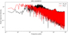 |
Fig. A.1. Power spectrum density of the HD 115427 (D) obtained for C6 light curves calibrated with EVEREST (in red) and with the adapted Lightkurve package (in black). |
For a more quantitative analysis, we first compared the background parameters of both Harvey models that we fitted: frequency (νc, Hi) and amplitude (AHi). We find that, for all stars, both parameters disagree by more than 1 σ. In the comparison of the noise parameter, a much higher level of noise is obtained for the light curve from C6LK.
For the case of HD 115427 (D), in addition to differences in the background parameters, the frequency of maximum power also differs by more than 1 σ. In the PSD, we can see that the p-mode ‘bump’ is wider with EVEREST than with Lightkurve. In addition, the fit of the Gaussian envelope is done on top of the background. If the backgrounds are different, this will also impact the fit of the Gaussian function on the p-mode envelope.
For the subgiant, HD 119026 (G), differences of greater than 1 σ are also observed in the comparison between the parameters νc, H2 and AGauss. Wenv is the width of the Gaussian envelope of the p modes. This larger difference for HD 115427 (D) indicates to us that the width of the envelope is greater in C6EV than in C6LK. In general, we find that the S/N is higher for the EVEREST light curves.
Finally, we look at the comparison of the parameters obtained from the Universal Pattern fit in apollinaire: ϵ, α, δν, νmax and Wenv. We find no significant differences between the two calibrations, which usually lay below the 3 σ level.
In conclusion, we find that the noise is higher in the light curve calibrated with Lightkurve compared to the EVEREST light curve. Therefore, we decided to use the C6EV light curve and combine it with the C17LK light curve for the full analysis of the K2 data available for our targets.
Appendix B: Effect of the gap removal on EPIC 212485100
Removing a long gap in the light curve produces a sudden break in the phase of the modes. On one hand, if the lifetime of the modes is shorter than the gaps, the phase of the mode is already broken and there is no effect on the properties of the mode. On the other hand, if the modes are long lived, that is longer than the gap, the phases are still coherent and the lifetime of the modes will be artificially reduced to the length of the segments. In other words, the modes will be widened. This effect was thoroughly studied using Monte Carlo simulations as well as long solar datasets in Section 4 of Ballot et al. (2004b) and in Section 5 of Ballot et al. (2004a). For the stars analyzed in this work, the thinnest modes have widths of around 1 μHz, corresponding to lifetimes of ∼3.7 days (see e.g., Eq. 24 in García & Ballot 2019). It is then clear that during the ∼880 days of the gap, the modes have been re-excited hundreds of times and thus the break in the phase that we have imposed by removing the gap has no effect on the limit spectrum of the modes.
Recently, in the paper by Bedding & Kjeldsen (2022), the authors investigated the impact of a gap in photometric data on characterization of solar-like oscillations. However, the authors did not correctly interpret the effect of the limit spectrum and the excitation function. In the seismic analysis of solar-like stars with stochastically excited modes, what is important is to characterize the underlying limit spectrum (the Lorentzian function) and not the effect of the excitation that multiplies it. Therefore, it is absolutely normal that the distribution of points around the limit Lorentzian function is different when comparing the PSDs of the series with and without the gap. When a Lorentzian fitting is performed on the PSD, the properties of the function are correctly retrieved regardless of the appearance of the exciting function.
Although Ballot et al. (2004a,b) already proved that it is perfectly correct to remove the gap for short-lived stochastic excited modes and study the resultant time series as a whole, we present here the analysis of simulated data based on one of the K2 targets, EPIC 212485100. We performed a 500 Monte Carlo simulation of the 11 longest lived modes in EPIC 212485100 (from l = 2 at ν = 1414.76 μHz up to l = 0 at ν = 1679.24 μHz) in the same conditions as in the K2 data analyzed in this paper, that is a total time span of 1029 days consisting of a first series of 79 days (similar to the C6 observations), a gap of 883 days and a final segment of 67 days (as in C17). The properties of the modes and the background used to build the limit spectrum were taken from the fit of the C06 EVEREST dataset. In Fig. B.1, the limit spectrum used to compute the Monte Carlo simulation is shown. Once this limit spectrum is calculated, we convert the PSD into an amplitude spectrum (AS) and we multiply the real and imaginary parts of the AS by two Gaussian noise distributions. By calculating the inverse Fourier transform, we obtain the 1079 day light curve associated with a single noise realization. Then we repeat the process 500 times.
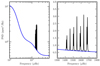 |
Fig. B.1. Monte Carlo simulations to probe the limit spectrum. Left panel: Limit spectrum of the 11 simulated modes based on EPIC 212485100 (black lines) as well as the contribution of the convective background and the photon noise (blue line). Right panel: Zoom onto the p modes. |
In the following, we describe the results obtained when studying the mode ℓ = 1, n = 16 at ν = 1546.656 μHz, which is placed at the center of the 11 simulated modes. The analysis of the other modes provides similar conclusions. Two cases were simulated: (a) the analysis of the first continuous 146 days of the simulated time series, that is, with no forced break of the phase; this is used as a reference for comparison; and (b) the analysis of the segment containing the last 67 days concatenated with the first segment after removing the gap, giving a total of 146 days as done in the analysis of the K2 real data. For both cases, the fitting with the apollinaire code was performed. Fig. B.2 shows the distribution of the fitted frequency (subtracted by the theoretical value of 1546.656 μHz) in orange for the continuous series with the red dashed line representing the fit of a Gaussian distribution to the data. The results for the gap-removed series are shown in blue, with the blue dashed line representing the theoretical Gaussian fit. The mean and the standard deviation of the Gaussian functions are -0.03 and 0.27, and -0.014 and 0.28, for cases (a) and (b), respectively. Thus, the difference between the centers of the distributions is zero inside the statistical uncertainties. There is no bias in the center of the distribution of the gap-removed series. Moreover, the standard deviation is also the same, proving that removing the gap has no effect on the characterization of the limit spectrum while having nearly twice the frequency resolution compared to either the analysis of each campaign separately or the average of both of them.
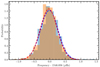 |
Fig. B.2. Histogram of the 500 Monte Carlo simulations of the frequencies of the fitted mode ℓ = 1, n = 16 after subtracting the theoretical value of ν = 1546.656 μHz. The results of the gap-corrected series are shown in blue, while the result of the light curve of the consecutive 146 day series is shown in orange. The dashed lines are the fitted Gaussian distributions as explained in the text. |
It is also important to emphasize that averaging the two campaigns is not a good solution, as suggested by Bedding & Kjeldsen (2022). As already mentioned, by doing so, the resolution will be degraded compared with the analysis of the concatenation of the two campaigns. The second problem would be associated with the change of the statistics when averaging two PSDs. In this case, the statistics of the averaged PSD is not a χ2 with 2 d.o.f. but a higher number of degrees of freedom. As a consequence, the error bars obtained from the fit need to be corrected as explained in Appourchaux (2003). Unfortunately, the correction factor provided by these latter authors was obtained for a Maximum likelihood minimization, while we are using a Bayesian approach. It is out of the scope of this paper to study this procedure in detail given that an alternative solution has been shown to be correct. Moreover, as zero padding is needed in the second campaign to reach the same length of 79 days as the first time series in order to have the same frequency resolution in the PSDs before averaging them, this implies the addition of a correlation between the points. Hence, the resulting statistical distribution of the PSD of the second campaign is already a χ2 with a higher degree of freedom, which will then modify the statistics of the final averaged PSD in a very different way from what was studied by Appourchaux (2003). In conclusion, it is not possible to asses the reliability of the inferred error bars in the Bayesian fit when averaging the PSDs of the two K2 campaigns considered here. Therefore, averaging the PSDs is not a valid methodology in our study.
Appendix C: Individual frequencies of the p modes
In this Appendix, we provide tables containing the results of the apollinaire fit for each star: the radial order, n, the mode degree, ℓ, and the frequency of the mode, νl, n, with the associated error. Mixed modes are those with an order n > 100. The column “flag” provides the list of modes used to find the best-fit stellar evolution models. A flag of 1 indicates that the mode was used, while 0 means that the mode was not used. The last column (“Fitted by Ong+21”) indicates whether or not the mode was fitted in Ong et al. (2021). Modes that were fitted by the latter have “Fitted by Ong+21 = 1” and new modes from our analysis are indicated by “Fitted by Ong+21 = 0”.
Individual frequencies for HD 115680 (A, EPIC 212478598).
Individual frequencies for HD 116832 (B, EPIC 212485100).
Individual frequencies for HD 114558 (C, EPIC 212487676).
Individual frequencies for HD 115427 (D, EPIC 212509747). This star has not been analyzed in Ong et al. (2021).
Individual frequencies for HD 120746 (E, EPIC 212516207).
Individual frequencies for HD 117779 (F, EPIC 212617037). This star has not been analyzed in Ong et al. (2021).
Individual frequencies for HD 119026 (G, EPIC 212683142).
Individual frequencies for HD 119038 (H, EPIC 212772187). This star has not been analyzed in Ong et al. (2021).
Appendix D: Echelle diagrams and models
In this Appendix, we show the echelle diagrams of the eight stars analyzed in this work, with the modes fitted by apollinaire (red circles) and the frequencies of the best-fit model (orange diamonds). For the model frequencies, only the most reliable modes used in the model fitting are represented, as explained in Section 5.2.
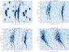 |
Fig. D.1. Echelle diagram of HD 115680 (A, EPIC 212478598), (top left panel); HD 116832 (B, EPIC 212485100), (top right panel); HD 114558 (C, EPIC 212487676), (bottom left panel); and HD 115427 (D, EPIC 212509747), (bottom right panel). The modes fitted by apollinaire are represented by red circles, while the orange diamonds correspond to the frequencies of the best-fit model after adding the surface corrections for the modes used as input. The magenta triangles represent the theoretical modes that were not part of the model-fitting procedure. Also, for the theoretical ℓ = 2 and 3 modes of HD 115680 (A, EPIC 212478598) star, only modes with a predominant p mode character are shown. |
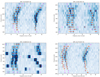 |
Fig. D.2. Echelle diagram of HD 120746 (E, EPIC 212516207), (top left panel); HD 117779 (F, EPIC 212617037), (top right panel); HD 119026 (G, EPIC 212683142), (bottom left panel); and HD 119038 (H, EPIC 212772187), (bottom right panel). Same legend as in Figure D.1. |
Appendix E: Frequency comparison with Ong et al. (2021)
As five of our targets (A, B, C, E, and G) were previously analyzed by Ong et al. (2021), we compare their frequencies (νn, l, Ong) –of the modes we have in common– with the ones obtained with apollinaire (νn, l, apo) using two K2 campaigns. In Figure E.1, we can see that there is good agreement for the modes in common between the two analyses. Most of the frequencies agree within 3 σ, except a couple of modes for star E where the agreement is around 4 σ.
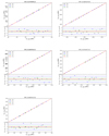 |
Fig. E.1. Comparison between the frequencies of modes in common obtained in this work (νn, l, apo) and those obtained in the analysis done by Ong et al. (2021), (νn, l, Ong). In the top panels, the red dashed line corresponds to the one-to-one line. In the bottom panels, we show the difference between the frequencies normalized by σ, which is computed as the square root of the quadratic sum of the frequency uncertainties from both methods. The green dash-dotted (blue dashed) lines correspond to ± 1 σ (± 3 σ). |
All Tables
Atmospheric and global seismic parameters for our sample of stars with their corresponding letter references from A to H.
Individual frequencies for HD 115427 (D, EPIC 212509747). This star has not been analyzed in Ong et al. (2021).
Individual frequencies for HD 117779 (F, EPIC 212617037). This star has not been analyzed in Ong et al. (2021).
Individual frequencies for HD 119038 (H, EPIC 212772187). This star has not been analyzed in Ong et al. (2021).
All Figures
|
Fig. 1. Comparison of the standard K2 aperture (left panel), the standard Lightkurve pipeline mask (middle panel), and our customized mask (right panel), taking pixels with an average flux larger than 1.4 × 10⁵ e− s−1 for HD 115680 (A). |
| In the text | |
|
Fig. 2. Ratio of the difference between the observed νmax and the estimation from EPIC data (black circles) and Gaia DR2 data (blue triangles), and the combined uncertainties, σ. The green dot-dashed lines correspond to ±1σ and the blue dashed lines represent the 3σ limits, where sigma is the square root of the sum of the quadratic errors. The red continuous line depicts the null difference. |
| In the text | |
|
Fig. 3. Seismic Hertzsprung-Russell diagram, where the luminosity is modified by the mean large frequency spacing, Δν. The colored symbols represent the stars studied here: red triangles are the main sequence stars; blue stars are stars near the TAMS; orange squares are subgiants. The Kepler sample with detected solar-like oscillations (Mathur et al. 2022) are also represented with gray circles. The evolutionary tracks with solar metallicity from the Aarhus STellar Evolution Code (Christensen-Dalsgaard 2008a) are represented with the black lines. The average uncertainties on Teff and Δν are shown in the lower left corner. |
| In the text | |
|
Fig. 4. Phase offset from the universal pattern fit of apollinaire, ϵ, as a function of Teff from Gaia DR2. The Kepler targets with characterized individual modes are represented with gray circles. MS stars in our sample, the two TAMS stars and the two subgiants are represented with red triangles, blue stars and orange squares, respectively. |
| In the text | |
|
Fig. 5. Stellar fundamental parameters obtained with models without diffusion for our K2 targets (referred to with letters A through H) showing mass vs radius (upper left panel), mass vs age (upper right panel), and age vs radius (lower left panel). In all panels, main sequence stars are represented by red triangles, stars close to the TAMS with blue stars, and subgiant/red giant stars with orange diamonds. For comparison, Kepler solar-like stars with detailed seismic modeling are represented with gray circles (Silva Aguirre et al. 2015, 2017), while subgiants are shown with dark gray squares (Li et al. 2020). |
| In the text | |
|
Fig. 6. Ages obtained with the IACgrid with diffusion vs ages from the IACgrid without diffusion (top panel). The one-to-one line is represented with the red dashed line. Ratio between the two different age computations as a function of the age from the IACgrid without diffusion (bottom panel). The red dashed line is the equality line while the gray dot-dashed lines correspond to the mean age uncertainty on stellar ages without diffusion of our sample (of 8%). |
| In the text | |
|
Fig. 7. Comparison between Gaia DR2 radii and radii from seismic modeling without using the luminosity constraint from Gaia for our eight targets. The red dashed line represents the one-to-one line. |
| In the text | |
|
Fig. A.1. Power spectrum density of the HD 115427 (D) obtained for C6 light curves calibrated with EVEREST (in red) and with the adapted Lightkurve package (in black). |
| In the text | |
|
Fig. B.1. Monte Carlo simulations to probe the limit spectrum. Left panel: Limit spectrum of the 11 simulated modes based on EPIC 212485100 (black lines) as well as the contribution of the convective background and the photon noise (blue line). Right panel: Zoom onto the p modes. |
| In the text | |
|
Fig. B.2. Histogram of the 500 Monte Carlo simulations of the frequencies of the fitted mode ℓ = 1, n = 16 after subtracting the theoretical value of ν = 1546.656 μHz. The results of the gap-corrected series are shown in blue, while the result of the light curve of the consecutive 146 day series is shown in orange. The dashed lines are the fitted Gaussian distributions as explained in the text. |
| In the text | |
|
Fig. D.1. Echelle diagram of HD 115680 (A, EPIC 212478598), (top left panel); HD 116832 (B, EPIC 212485100), (top right panel); HD 114558 (C, EPIC 212487676), (bottom left panel); and HD 115427 (D, EPIC 212509747), (bottom right panel). The modes fitted by apollinaire are represented by red circles, while the orange diamonds correspond to the frequencies of the best-fit model after adding the surface corrections for the modes used as input. The magenta triangles represent the theoretical modes that were not part of the model-fitting procedure. Also, for the theoretical ℓ = 2 and 3 modes of HD 115680 (A, EPIC 212478598) star, only modes with a predominant p mode character are shown. |
| In the text | |
|
Fig. D.2. Echelle diagram of HD 120746 (E, EPIC 212516207), (top left panel); HD 117779 (F, EPIC 212617037), (top right panel); HD 119026 (G, EPIC 212683142), (bottom left panel); and HD 119038 (H, EPIC 212772187), (bottom right panel). Same legend as in Figure D.1. |
| In the text | |
|
Fig. E.1. Comparison between the frequencies of modes in common obtained in this work (νn, l, apo) and those obtained in the analysis done by Ong et al. (2021), (νn, l, Ong). In the top panels, the red dashed line corresponds to the one-to-one line. In the bottom panels, we show the difference between the frequencies normalized by σ, which is computed as the square root of the quadratic sum of the frequency uncertainties from both methods. The green dash-dotted (blue dashed) lines correspond to ± 1 σ (± 3 σ). |
| In the text | |
Current usage metrics show cumulative count of Article Views (full-text article views including HTML views, PDF and ePub downloads, according to the available data) and Abstracts Views on Vision4Press platform.
Data correspond to usage on the plateform after 2015. The current usage metrics is available 48-96 hours after online publication and is updated daily on week days.
Initial download of the metrics may take a while.