© M. Briday et al. 2021

1. Introduction

Type Ia supernovae (SNe Ia) are powerful empirically standardized distance indicators. They enabled the discovery of the acceleration of the expansion of the Universe (Riess et al. 1998; Perlmutter et al. 1999), and today are still key cosmological probes in the context of the new generation of surveys (Scolnic et al. 2019). SNe Ia play an important role in probing the nearby Universe (z < 0.3) and are the last step of the direct distance ladder to derive the Hubble-Lemaître constant H₀ (e.g., Freedman et al. 2001; Riess et al. 2009). Interestingly, when calibrating the SNe Ia absolute luminosity using the Cepheid period–luminosity relation, this direct H₀ measurement is 4.4σ higher than expectation based on the Lambda cold dark matter (ΛCDM) model anchored by Planck Collaboration VI (2020) data (Riess et al. 2019; Reid et al. 2019). This “tension” has received a great deal of attention as it could be a sign of new fundamental physics (Knox & Millea 2020). This finding is supported by analyses of strongly lensed quasars that are also reporting high H₀ measurements (e.g., Wong et al. 2020). However Freedman et al. (2019) find a lower H₀ value when using tip of the red giant branch (TRGB) distances in place of the Cepheids.

This raises the question of systematic uncertainties affecting direct H₀ measurements in particular, and the distances derived from the observation of the SNe Ia in general. Rigault et al. (2015) suggests that an unaccounted for astrophysical bias, affecting the derivation of the absolute SNe Ia luminosity, could explain at least part of the tension. The SNe Ia from the calibrating sample significantly differ from the Hubble flow ones; those in the calibrating sample are selected such that their host galaxy also contains Cepheid stars and are thus star forming. Rigault et al. (2020) claim that SNe Ia from younger environments are 0.16 mag fainter than those from older environments, leading to a bias on H₀ because of this selection effect. Even so, Riess et al. (2019) have mimicked the Cepheid selection function onto the Hubble flow sample and find no variation in H₀, suggesting that they are not affected by this astrophysical effect (see also Jones et al. 2015).

After more than a decade of analyses, the amplitude and the root causes of the astrophysical biases affecting the distance measurements from SNe Ia remain unclear. Early Ia rate studies have shown evidences that two populations of SNe Ia may exist: one arising from young (< 100 Myr) progenitor systems and one related to older (Gyr), most evolved progenitors (i.e., the A+B or prompt and delayed models; see e.g., Mannucci et al. 2005, 2006; Scannapieco & Bildsten 2005; Sullivan et al. 2006; Aubourg et al. 2008; Smith et al. 2012; Maoz et al. 2014; Rodney et al. 2014). The first significant evidence of an astrophysical bias in the SN distance derivations was the observed dependency of the standardized SNe Ia magnitude (using the classical two-parameter light curve standardization method) with host galaxy stellar mass (e.g., Kelly et al. 2010; Sullivan et al. 2010; Lampeitl et al. 2010; Gupta et al. 2011; Childress et al. 2013b; Betoule et al. 2014; Uddin et al. 2017; Ponder et al. 2020): SNe Ia from massive galaxies (M_* > 10¹⁰ M_⊙) are brighter, after standardisation, by ∼0.1 mag.

We use the term magnitude-step to describe the difference in average standardized magnitudes between two SN Ia subsamples defined from an environmental tracer cutoff. This simple functional form has been shown by Childress et al. (2013b) to be the best fit to data in comparison to a linear trend or other theoretically inspired forms. We further highlight that, in practice, this data-driven step implies that there are two populations of ‘SN Ia+environment’ that are simultaneously present; this observation is the central point of this paper.

The term mass-step has been extensively used in the literature for the global host-stellar mass tracer. The mass-step is used as a third standardization parameter in many recent SNe Ia cosmological analyses (Sullivan et al. 2010; Betoule et al. 2014; Scolnic et al. 2018), including the direct H₀ measurements from Riess et al. (2016, 2019). The amplitude of this effect is ∼0.08 mag. However, the underlying physics causing this magnitude dependency, and the proper way to account for such astrophysical biases, remain unclear.

In the last decade many host environmental studies seem to have converged towards either the age of the progenitor, or dust around the progenitor or in the host interstellar medium as the origin of the mass-step. Rigault et al. (2013, 2020), Roman et al. (2018), Kim et al. (2018) and Kelsey et al. (2021) would suggest age, while others, like Brout & Scolnic (2021), suggest that variable dust extinction curves affecting the observed color of the supernova can explain correlations with host galaxy properties. Rigault et al. (2020) show the most significant correlation between the luminosity of the SN and the properties of the environment. They split their SNe Ia as a function of the specific star formation rate (sSFR) derived from Hα flux measured within a 1 kpc radius projected onto the local environment around the SN (local sSFR; lsSFR). The SNe Ia having a large lsSFR, hence a large fraction of young stars in their vicinity, are fainter than those from passive local environments by 0.163 ± 0.029 mag. Since high-mass galaxies favor older stellar populations, massive hosts favor SNe from old environments, and so are, on average, brighter after light curve standardization, resulting in the mass-step.

Surprisingly, while most SN samples now observe significant correlation between host properties and standardized SN magnitudes, the magnitude step amplitudes differ and seem incompatible. For instance, the Supernova Legacy Survey (SNLS) five-year data and the Sloan Digital Sky Survey (SDSS) data from Roman et al. (2018), updating the Joint Light-curve Analysis (JLA) catalog from Betoule et al. (2014), find a local U-V step of 0.091 ± 0.013 mag, seemingly incompatible with Rigault et al. (2020). Jones et al. (2018), using the low-redshift bin of the Pantheon dataset (Scolnic et al. 2018), reported that locally massive environments (i.e., having a large surface density of stars) are fainter by 0.067 ± 0.017 mag. While in agreement with the local mass-step reported in Rigault et al. (2020, 0.059 ± 0.024 mag), this effect is significantly weaker than that observed using the lsSFR indicator. Finally, using the Pantheon dataset Pruzhinskaya et al. (2020) found that SNe Ia from elliptical and lenticular galaxies are brighter (0.058 ± 0.019 mag), in agreement with Kim et al. (2019, using JLA, 0.018 ± 0.052 mag) and Henne et al. (2017, 0.04 ± 0.05 mag).

As already pointed out by Jones et al. (2018), this variety of results, made using different host tracers, local or global, brings confusion about how to best account for astrophysical biases in SN cosmology, and notably on the derivation of H₀. In this paper we try to clarify the situation by studying how well each environmental indicator is able (or not) to trace a given environmental property.

We start in Sect. 2 by presenting that, mathematically, if two SN Ia populations were to exist, the observed amplitude of their true standardized magnitude difference linearly depends on the ability of a tracer to accurately measure which population a SN belongs to. We present in Sect. 3 the data sample we use for this work, and we describe the methodology used to extract the measurements of the environmental tracers. Then we apply in Sect. 4 our two-populations model on these data and we present our findings in Sect. 5, comparing them with results from the literature. For this we used the Hα-based lsSFR tracer as reference, and we test this hypothesis in Sect. 6. We discuss our findings and we conclude in Sect. 7.

2. The two-populations model

As discussed in the introduction, many SN cosmological analyses use step functions to account for environmental dependencies in the derivation of distances. These steps are the difference of average properties, for example q, between two sides of a boundary t_cut in a considered environmental property t. When applied to the previously mentioned mass-step, it corresponds to the difference of absolute magnitude (q is the magnitude) of SNe Ia from low- and high-mass hosts (t is the host stellar mass), conventionally split at the host stellar mass of t_cut = 10¹⁰ M_⊙.

The underlying assumptions when using a step function are the following: (1) there are two categories of SNe, for example a and b, that differ on average in q and (2) the tracer t is able to probe these categories. Consequently, the amplitude of the observed step depends on the intrinsic SN properties q and the quality of the tracer t.

In the following subsections, we describe our statistical model starting from an illustrative mock example, first explaining the mathematical concept without measurement errors, and then including them in the model, to finally introduce the probability function. A detailed mathematical derivation is given Appendix A.

2.1. Concept of contamination

Let us assume that the two SN populations a and b have a normally distributed quantity q, for example 𝒩_a = 𝒩(μ_a, σ_a) and 𝒩_b = 𝒩(μ_b, σ_b), for which they differ on average by γ₀ = μ_a − μ_b; this difference corresponds to the true step amplitude.

We now assume that we have access to a tracer t that is able to discriminate between the a and b populations, but not with perfect accuracy (using the statistical binary classification terminology, that is with neither perfect specificity nor sensitivity). The tracer classification is based on the cutoff value t_cut such that the SNe are classified as a or b if they are either above or below the cut, respectively.

Even assuming this tracer provides error-free measurements, we expect misclassifications from the tracer inaccuracy: some SNe from the a category will be measured below the t_cut and will thus be incorrectly classified as b, and vice versa.

This is illustrated in Fig. 1 for three cases with varying accuracy: perfect, medium, and null. This figure also illustrates how the estimation of the underlying q distribution for each a and b category is affected by the tracer’s inaccuracy, and consequently how the derived steps are potentially underestimated. As the tracer accuracy degrades and misclassification cases increase, the number of category a SNe incorrectly classified by the tracer as b increases (blue circles in the left part of the figure); similarly, the fraction of category b SNe misclassified as a also increases (orange circles in the right part of the figure). As a consequence of misclassifications, the measured distributions of q for each of the inferred populations a and b broaden and their means converge, so that the step measured using an inaccurate tracer is systematically smaller than the true step.

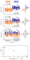Fig. 1. Concept of tracer purity and its impact on the step measurement of an arbitrary quantity q. Top three panels: 400 mock data, 200 of category a (in blue), normally distributed over the quantity q by 𝒩(μa = 0.5, σa = 0.5), and 200 of category b (in orange) with a similar distribution 𝒩(μb = −0.5, σb = 0.5). The figure shows the mock q values as a function of the tracer values t for three different tracers. The data are classified as a or b given the tracer values if they are measured above or below tcut, respectively. The top, middle, and bottom panels show tracers with perfect, medium, and null ability to track the two categories. The right panels show the tracer estimation of the q distribution for each tracer (in gray), to be compared to the true q distribution for each category (colored dashed lines). Bottom panel: evolution of the observed step γ = μa − μb, the difference of mean q values for targets classified as a or b by the tracers, as a function of the tracer contamination c = ca + cb; the circles show each of the three simulations illustrated in the top panels, while the line shows the prediction from Eq. (3).

2.2. Notations and definitions

For clarity, we set here our definitions and nomenclature in the large-number limit. N is the number of targets, the subscript _x denotes true conditions (x = {a; b}) and the superscript ^x denotes actual classifications by a tracer. Hence, $N_a^b$ is the number of targets that are truly a but classified as b. Accordingly, $N^b=N_a^b+N_b^b$ is the number of targets classified as b by a tracer, and $N_b=N_b^b+N_b^a$ is the number of targets that are intrinsically b.

We call contamination the fraction of targets for which the tracer classification differs from the truth. It could either be defined as the fraction $c_a\equiv N_a^b/N_a$ of truly a targets classified as b (resp. $c_b\equiv N_b^a/N_b$) or as the fraction $c^a\equiv N_b^a/N^a$ of classified a targets that actually are b (resp. $c^b\equiv N_a^b/N^b$). The two definitions are related as c^a = N_b/N^a c_b and c^b = N_a/N^b c_a. We also note that $1-c_x\equiv N_x^x/N_x$ and $1-c^x\equiv N_x^x/N^x$, where x is either a or b¹.

The probability p^a of a target tracer t_i to be measured above the tracer threshold t_cut, thus classified as a, is the sum of (1) the probability that a target truly is a and properly identified as a, and (2) the probability that it truly is b but misclassified as a:

$$\begin{array}{cc}& p^a\equiv \frac{N^a}{N}=\frac{N_a^a}{N}+\frac{N_b^a}{N}=(1-c_a)\times \frac{N_a}{N}+c_b\times \frac{N_b}{N}\hfill \\ \hfill & =(1-c_a)\times p_a+c_b\times (1-p_a)\hfill \end{array}$$(1)

where p_b ≡ N_b/N = 1 − N_a/N ≡ 1 − p_a. Similarly:

$$\begin{array}{cc}\hfill p^b& =c_a\times p_a+(1-c_b)\times (1-p_a).\hfill \end{array}$$(2)

While μ_a and μ_b are the true means of the SN from categories a and b, respectively (see Sect. 2.1), μ^a and μ^b are the distribution means of the considered distributions for each group classified by the tracer (filled gray distributions in Fig. 1). Accordingly, the observed amplitude step γ = μ^a − μ^b, as measured by a tracer, is related to the true intrinsic step γ₀ = μ_a − μ_b by

$$\begin{array}{cc}& \gamma =((1-c^a){\mu }_a+c^a{\mu }_b)-(c^b{\mu }_a+(1-c^b){\mu }_b)\hfill \\ \hfill & ={\gamma }_0\times [1-(c^a+c^b)].\hfill \end{array}$$(3)

This prompts us to define the (total) contamination of a tracer as c = c^a + c^b. The linearly decreasing relation in the bottom panel of Fig. 1 illustrates this equation.

2.3. Reference, comparison tracers, and measurement errors

It is unlikely to have access to the true population classification; instead it is necessary to rely on a reference tracer with respect to which the other tracers can be compared. This reference tracer is itself an observable associated with its own contamination parameters $c_a^{\text{ref}}$ and $c_b^{\text{ref}}$; however, in this analysis, we will generally consider a perfectly accurate reference tracer: $c_a^{\text{ref}}=c_b^{\text{ref}}=0$. The correlation of any other tracer with respect to this reference tracer enables the contamination of this comparison tracer to be derived.

This is illustrated in Fig. 2. In the case of error-free measurements (top two panels), the contamination will simply be the fractions of off-diagonal terms of the correlation plot between the reference tracer and the comparison tracer. However, measurement uncertainties complicate the picture as they randomly scatter points into the off-diagonal parts of the plot, even in the case of a perfect tracer, as illustrated in the bottom panel of the figure.

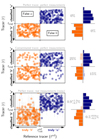Fig. 2. Correlation between uniform mock reference and comparison tracers. The color indicates the true classification following the color-coding in Fig. 1: blue for a, orange for b. The right panel of each row shows the marginalized distribution of each quadrant, following the color-coding of the circles. The light histograms correspond to the off-diagonal terms: false a in light orange, false b in light blue. Top panels: perfect and noise-free tracer, i.e., without any off-diagonal points; middle panels: imperfect (ca = 15% and cb = 25%) yet noise-free tracer, the sum of its off-diagonal terms corresponds to its contamination parameters; bottom panels: perfect but noisy tracer. In this case, plain off-diagonal fractions are 11% in false a and 7.5% in false b, while both should be 0% for a perfect tracer; the likelihood estimator (Eq. (11), see Sect. 2.4), properly accounting for the fraction of off-diagonal terms caused by measurement errors, provides contamination estimates $c_a=0.5_{-0.3}^{+0.8}\%$ and $c_b=0.9_{-0.7}^{+1.3}\%$, compatible with zero.

We denote f_i as the probability that a given tracer measurement t_i ± δt_i is below the cutoff value t_cut (and therefore the target is classified as b). Then f_i is expressed (for normally distributed errors) as

$$\begin{array}{c}\hfill f_i=\mathcal{P}(t_i<t_{\mathrm{cut}})={\displaystyle {\int }_{-\infty }^{t_{\mathrm{cut}}}\mathcal{P}({\widehat{t}}_i\mid t_i)\mathrm{d}{\widehat{t}}_i={\int }_{-\infty }^{t_{\mathrm{cut}}}\mathcal{N}({\widehat{t}}_i;t_i,\delta t_i)\mathrm{d}{\widehat{t}}_i}\end{array}$$(4)

where ${\widehat{t}}_i$ correspond to the true value of t_i.

By definition, we then have N^b ≡ ∑f_i and N^a ≡ ∑(1 − f_i); similarly, the number of off-diagonal elements are $N_a^b=\sum _{i\in a}{f}_i$ and $N_b^a=\sum _{i\in b}(1-f_i)$. Therefore, even in the context of a perfect tracer (for which we expect c_a = c_b = c^a = c^b = 0), the previous simple contamination estimates of $c^a=N_b^a/N^a$ or $c^b=N_a^b/N^b$ can appear to be non-zero due to measurement uncertainties, and can degrade the intrinsic tracer contamination estimates.

Instead, c^a and c^b should be estimated as the fractions of off-diagonal terms that are not caused by measurement errors. This will be done by defining the probability function, and comparing it to observations.

2.4. Building the probability function to estimate c^a and c^b

In order to get the contamination of a tracer (c = c^a + c^b; see Sect. 2.2), we first express the probability function of the intrinsic parameters c_a and c_b.

Following the derivations presented in Appendix A, we can express the probability of measuring t_i when the target i belongs to population b as

$$\begin{array}{c}\hfill \mathcal{P}(i\in b,t_i\mid c_b)\propto (1-p_a)((1-c_b)\times f_i+c_b\times (1-f_i)).\end{array}$$(5)

This can be understood as the probability that a target is b (i.e., (1 − p_a)) times the chance that a tracer is measured below a cut (f_i), and thus classifying the target as b, while accounting for the fraction of false negatives (1 − c_b), plus the chance that the tracer is measured above the cut (1 − f_i) times the fraction of false positives (c_b).

Similarly for the probability of measuring t_i when the target i belongs to population a,

$$\begin{array}{c}\hfill \mathcal{P}(i\in a,t_i\mid c_a)\propto p_a(c_a\times f_i+(1-c_a)\times (1-f_i)),\end{array}$$(6)

and therefore

$$\begin{array}{cc}& \mathcal{P}(t_i\mid c_a,c_b)=\mathcal{P}(i\in a,t_i\mid c_a)+\mathcal{P}(i\in b,t_i\mid c_b)\hfill \\ \hfill & \propto p_a\times ((1-c_a)\times (1-f_i)+c_a\times f_i)\hfill \\ \hfill & +(1-p_a)\times (c_b\times (1-f_i)+(1-c_b)\times f_i).\hfill \end{array}$$(7)

As mentioned in Sect. 2.3, in reality, we do not know if an individual target belongs to class a or b: the contamination cannot be directly tied to the truth, but only to another tracer used as a reference, plagued by its own contamination and measurement errors. Using ^ref to denote the parameters for the reference tracer, p_a and p_b = 1 − p_a, which cannot be estimated directly anymore, can be derived from the reference tracer as

$$\begin{array}{cc}& p_a\equiv \mathcal{P}(i\in a,t_i^{\mathrm{ref}}\mid c_a^{\mathrm{ref}})\hfill \\ \hfill & =p_a^{\mathrm{ref}}\times ((1-c_a^{\mathrm{ref}})\times (1-f_i^{\mathrm{ref}})+c_a^{\mathrm{ref}}\times f_i^{\mathrm{ref}})\hfill \end{array}$$(8)

and

$$\begin{array}{cc}& p_b\equiv \mathcal{P}(i\in b,t_i^{\mathrm{ref}}\mid c_b^{\mathrm{ref}})\hfill \\ \hfill & =(1-p_a^{\mathrm{ref}})\times (c_b^{\mathrm{ref}}\times (1-f_i^{\mathrm{ref}})+(1-c_b^{\mathrm{ref}})\times f_i^{\mathrm{ref}}).\hfill \end{array}$$(9)

where $p_a^{\text{ref}}$, the fraction of truly a targets, have to be assumed a priori since the reference tracer is noisy (see Sect. 4).

Assuming the reference tracer to be perfect (i.e., $c_a^{\text{ref}}=c_b^{\text{ref}}=0$), Eq. (7) becomes

$$\begin{array}{cc}& \mathcal{P}(t_i,t_i^{\mathrm{ref}}\mid c_a,c_b)\propto \hfill \\ \hfill & p_a^{\mathrm{ref}}\times (1-f_i^{\mathrm{ref}})\times ((1-c_a)\times (1-f_i)+c_a\times f_i)\hfill \\ \hfill & +(1-p_a^{\mathrm{ref}})\times f_i^{\mathrm{ref}}\times (c_b\times (1-f_i)+(1-c_b)\times f_i).\hfill \end{array}$$(10)

Finally, the estimation of the tracer’s parameters c_a and c_b with respect to the reference tracer is made by minimizing

$$\begin{array}{c}\hfill \mathcal{L}=-2{\displaystyle \sum _{i}ln\mathcal{P}(t_i,t_i^{\mathrm{ref}}\mid c_a,c_b),}\end{array}$$(11)

and the total contamination c = c^a + c^b for a comparison tracer can be computed from

$$\begin{array}{cc}& c^a=\frac{N_b}{N^a}{c}_b=\frac{(1-p_a^{\mathrm{ref}})N}{\sum (1-f_i)}{c}_b\hfill \\ \hfill & c^b=\frac{N_a}{N^b}{c}_a=\frac{p_a^{\mathrm{ref}}N}{\sum f_i}{c}_a.\hfill \end{array}$$(12)

We tested and validated our model and our code using simulations. We generated mock datasets of various contaminations and sizes, which were fitted with our implementation of the likelihood described in this section. The results confirm that our implementation of the algorithm is correct.

3. Data

We work with the Nearby Supernova Factory (SNfactory, Aldering et al. 2002) SNe Ia dataset published in Rigault et al. (2020) (see also Aldering et al. 2020). This dataset has two advantages for this analysis: it is at low redshifts (0.02 < z < 0.08), so the local environment is measurable, and it contains spectrophotometric integral field units (IFU) environmental data, necessary to accurately estimate the local specific star formation rate (lsSFR). We use the publicly available catalog and images from SDSS and PanStarrs for the photometric measuments or their derived quantities.

This section briefly summarizes the methodology used to extract the different tracers considered in this analysis, which follows those developed in the literature, namely: the spectroscopically derived lsSFR (Sect. 3.1), photometrically derived lsSFR (Sect. 3.6), local colors (Sect. 3.4), local and global host stellar masses (Sect. 3.5), and the global host morphologies (Sect. 3.7).

3.1. Spectroscopic lsSFR

The spectroscopically derived lsSFR is detailed in Sect. 3 of Rigault et al. (2020). We use their measurements, which are generated in two stages: first, the star formation rate (SFR) is derived from the Hα emission line luminosity (Calzetti 2013), spectroscopically measured within the local 1 kpc aperture radius, after subtraction of the stellar continuum background. The second step is the measurement of the local stellar mass, as described in Sect. 3.5. For both quantities, a full posterior distribution is derived such that their ratio sets the posterior distribution of the lsSFR measurements. Hereafter, we will refer to this tracer as the spectroscopic lsSFR.

3.2. Photometric measurements

We used flux-calibrated optical images from SDSS (DR12, Alam et al. 2015) to derive the photometric environmental tracers.

We measured ugriz SDSS local fluxes and their uncertainties in projected circular apertures centered on the SN location, using the SUM_CIRCLE method of SEP² (Barbary 2016). To compare our results with those of literature studies, we used aperture radii of X = 1, 1.5, and 3 kpc. Counts were converted to flux assuming a zero point of 22.5 mag for the gri bands, and 22.46 and 22.52 for the u and z bands, respectively.

To test the accuracy of the sky background subtraction, we drew 500 random source-free apertures around each target. Presumably, the histogram of the error-normalized background levels should be a standard 𝒩(0, 1) pull distribution. However, we regularly observed that the pull mean was slightly too high, corresponding to an inaccurate background correction, and that the pull dispersion was larger than unity, meaning that the error on the background level had been under-estimated. We thus further corrected each aperture photometric measurement by the median of the 500 random sky apertures, and scaled the quoted error by the normalized median absolute deviation of the sky levels.

To derive global tracers, we first associated the SN with its host employing the directional light radius method (Sullivan et al. 2006; Gupta et al. 2016); ellipses used to determine the directional light radius were obtained by the SUM_ELLIPSE method of SEP. Then we used the ugriz global galaxy model magnitudes and fluxes from the corresponding SDSS catalog entries (see details in Rigault et al. 2020).

Both local and global photometric measurements were then corrected for Milky Way dust absorption using the EXTINCTION³ library assuming a Fitzpatrick (1999) extinction curve with R_V = 3.1 and the dust extinction map from Schlegel et al. (1998).

3.3. SED fitting and k-correction

From each ugriz photometric dataset, we used LEPHARE⁴ (Arnouts et al. 1999; Ilbert et al. 2006; Arnouts & Ilbert 2011) to fit for the associated spectral energy distribution (SED) using templates from Bruzual & Charlot (2003) (hereafter BC03) as did Jones et al. (2018), among others. For the reproducibility, our configuration file is available online⁵. It contains the following assumptions:

The SED fit was made at the fixed (known) redshift of the host, the stellar mass M_* was bounded between 10⁶ and 10¹³ solar masses, and the r-band absolute magnitude between −10 and −26. We included the SDSS suggested error floor (0.05, 0.02, 0.02, 0.02, 0.03 for the ugriz bands (see, e.g., kcorrect.org and Childress et al. 2013a).

We estimated the posterior distribution of each SED fitted parameter and spectrum using Monte Carlo simulations. For each ugriz flux measurement (i.e., for each local radius of each SN) we randomly drew 500 realizations assuming that the bands are independent and that flux errors are normally distributed. We ran the SED fitting procedure for these 500 realizations and the best fitting parameters ( _BEST) and spectral distributions were used to fix the respective posteriors. We used the median rest-frame magnitudes measured on each of the 500 realizations to estimate the ugrizk-corrected magnitudes used in this analysis; the 16% and 84% percentiles indicate the corresponding errors.

3.4. Colors

The colors were estimated from the k-corrected magnitudes (see Sect. 3.3): the u − r color is the difference of the median of the k-corrected u- and r-band magnitudes, and the color error is the quadratic sum of the individual standard deviations.

3.5. Stellar masses

Local and global masses were derived using the procedure described in Sect. 3.3 of Rigault et al. (2020) (see also Jones et al. 2018). In brief, we use the relation from Taylor et al. (2011) to convert g and ik-corrected magnitudes into stellar masses. This relation has a 0.1 dex intrinsic dispersion that is added in quadrature to the stellar mass uncertainties derived from photometric uncertainties alone; this scatter dominates the error budget, especially for global measurements (see Smith et al. 2020 for a discussion about the consistency of stellar mass estimators in the context of SN host analyses).

3.6. Photometric lsSFR

Jones et al. (2018) use photometry-based sSFR estimations to assess the lsSFR parameter in place of the Hα-based measurements as they do not have local spectroscopy. They employ LEPHARE in a similar fashion to that described in Sect. 3.3 and estimate their sSFR posterior (and its errors) from the 50% ([16%, 84%]) of the individual sSFR values from the Monte Carlo realizations. They use the SDSS u-band plus grizy from PanStarrs DR1 (PS1, Chambers et al. 2016) to do so. To be consistent, when deriving the sSFR, we also used these data, applying the same photometric measurement on PS1 data as we did for SDSS (see Sect. 3.2). Calibrated PS1 images were downloaded from the cutout service⁶. Again for consistency, we also used the Jones et al. (2018)’s LEPHARE configuration file when measuring the sSFR this way (D. Jones, priv. comm.). The measurements were finally normalized by the surface area. Hereafter we refer to this tracer as the photometric lsSFR, in contrast to the spectroscopic lsSFR.

3.7. Morphology

The inverse concentration index (i.c.i., Shimasaku et al. 2001; Strateva et al. 2001, see also the SDSS web site) is a commonly used morphological tracer. It is the ratio of radii containing 50% and 90% of the Petrosian flux in r-band. With this tracer, early-type galaxies typically have an i.c.i.∼0.3, while late-type galaxies have an i.c.i. closer to 0.45. Following Kauffmann et al. (2003), we used i.c.i._cut = 1/2.7 = 0.37 to distinguish between late- and early-type galaxies (also see, e.g., Choi et al. 2010). Using slightly lower boundaries, such as 0.35 suggested by Banerji et al. (2010), among others, has marginal influence on our results.

Galaxy classification based on the Petrosian flux is one approach, but it is not the only one. Among a few others, the i.c.i. is the most convenient for this analysis as it discriminates between two galaxy morphology populations (early and late types) separated by a cutoff value, which motivates our choice.

4. Contamination with respect to the spectroscopic lsSFR

Because the sSFR is usually used as a reference age tracer when available (see, e.g., Yoshikawa et al. 2010; Labbé et al. 2013; Casado et al. 2015; Karman et al. 2017), we used the spectroscopic lsSFR measurement from Rigault et al. (2020) as a reference tracer, assuming that this quantity is a perfectly accurate (yet imprecise) progrenitor age tracer: $c_{\text{spec-lsSFR}}^a = c_{\text{spec-lsSFR}}^b = 0$ (see Sect. 2). We test this hypothesis in Sect. 6.2.

Following most of the preceding host environmental studies, which split their samples at the median value, we also assume throughout the paper that $p_a^{\text{ref}}$ = 50%. We have found by simulations that the derivation of the c_a and c_b tracer parameters are unaffected by this choice (bias lower than the 1σ error), as long as the actual true parameter $25\%\lesssim p_a^{\text{ref}}\lesssim 75\%$, which is to be expected simply based on rate analyses (e.g., Mannucci et al. 2006; Rodney et al. 2014; Wiseman et al. 2021); the bias becomes significant (at more than 3σ) if p_a < 10% or p_a > 90%.

4.1. Comparing the environmental tracers with the spectroscopic lsSFR.

Following Rigault et al. (2020), we classify as population a every SNe Ia with log(spec − lsSFR) > − 10.82 dex as this value corresponds to the median of this tracer for the SNfactory sample. Given the measurement errors, each SN Ia therefore has a probability p(young) of being observed in population a (referring to $1-f_i^{\text{ref}}$ in Sect. 2.4). As highlighted in Sect. 2.3, the sum of the off-diagonal terms are fully captured by the measurement errors since we assumed $c_{\text{spec-lsSFR}}^a=c_{\text{spec-lsSFR}}^b=0$.

Each tracer has its own cutoff value to classify a given SN Ia in population a. We apply the assumption typically used in the literature when available and the median value otherwise, which is usually also the literature assumption. The well-studied mass step usually has the threshold boundary set at log(M_*/M_⊙)_cut = 10 dex (e.g., Kelly et al. 2010; Sullivan et al. 2010; Betoule et al. 2014; Scolnic et al. 2018) and we use this value in this analysis. We note that since we have ∼60% of SNe Ia with a host-mass greater than 10¹⁰ M_⊙ (in agreement with, e.g., Roman et al. 2018), and since N_a/N is given by the reference tracer (here $p_a^{\text{ref}}=50\%$), this means that $c_{\text{gmass}}^a\ne c_{\text{gmass}}^b$. Concerning the local mass, Jones et al. (2018) and Rigault et al. (2020) use the median to divide their respective samples. For the sample here we find the median to be log(M_*/M_⊙)_cut = 8.37 dex; to compare with Jones et al. (2018), we used a 1.5 kpc “local” aperture for the local mass. Following Roman et al. (2018), Jones et al. (2018), and Kelsey et al. (2021), we did the same for the local (3 kpc) color and the photometric local (1.5 kpc) sSFR finding medians at u − r = 1.74 mag and log(phot − lsSFR) = − 10.32 dex, respectively. Finally, as explained in Sect. 3.7, we used i.c.i. = 0.37 to divide the morphologies of our SN Ia host galaxies into category a or b when respectively above or below this value.

In Fig. 3 we show the correlation between the spectroscopic lsSFR and the other environmental tracers. We first note that all tracers correlate relatively well with the spectroscopic lsSFR. Based on the Spearman rank coefficient, the most correlated tracer is the local u − r color (|ρ| = 0.71) closely followed by the global mass (|ρ| = 0.64); the host galaxy morphology and the local stellar mass show weaker correlations, with |ρ| = 0.45 and 0.32, respectively.

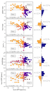Fig. 3. Correlation between each environmental tracer and the spectroscopic lsSFR, as mentioned in Sect. 4. The vertical gray line is the spectroscopic lsSFR cutoff, set at log(lsSFR) = − 10.82 dex. The horizontal gray lines are the other tracer cutoffs, as defined in Sect. 4. Each figure indicates the false a and false b classification quadrants. The color of the circles, which vary from orange to blue, represents the probability for a SN Ia to be in population a (blue) or b (orange) from the spectroscopic lsSFR point of view, whereas the edge color represents the same probability, but from the comparison tracer point of view. In the right column, the histograms plot the distributions in each quadrant. Orange (resp. blue) bars correspond to the truly b (resp. a) spectroscopic lsSFR classification. The estimated ca and cb parameters are given in percentages within the corresponding quadrants where the histogram is transparent.

The population of off-diagonal terms appear to be consistent with these Spearman-ranked correlations: the higher the fraction of off-diagonal terms, the lower the Spearman coefficient value. However, as detailed in Sect. 2.3, only the fraction of off-diagonal terms not caused by measurement errors has to be accounted for to measure the accuracy of an indicator to trace the reference, here the spectroscopic lsSFR.

To do that, we fit the parameters c_a and c_b of the tracers, assuming that the spectroscopic lsSFR measurements are (noisy) perfectly accurate indicators of a and b, by minimizing Eq. (11). Since the measurements are noisy, we need to set the fraction of truly a, that we assume to be 50% (i.e., we fix N_a = N_b). The fit is made using Markov chain Monte Carlo routines using the EMCEE (Foreman-Mackey et al. 2013) package to sample the full posterior distributions of the parameters c_a and c_b of the tracers. Each tracer is fitted independently. The resulting median parameters c^a and c^b are displayed in Fig. 3 with their 1σ scale (16%/84%), and the aggregated tracer contamination c = c^a + c^b is summarized in Table 1.

4.2. Measuring the environmental magnitude step

To derive the SNe Ia magnitude steps, we follow the procedure detailed in Sect. 4.2.2 of Rigault et al. (2020). Given $p_i^t=1-f_i^t$ the probability that the tracer measurement is above the tracer’s cutoff value (see Sect. 2.3), thus classified as a by this tracer, we fit the magnitude offset γ between the two populations (i.e., the step) together with the stretch and color standardization coefficients α and β. This is done by χ² minimization between μ_ΛCDM and the standardized SN Ia distance modulus:

$$\begin{array}{c}\hfill \mu =m-M+\alpha x_1-\beta c+\gamma p^t.\end{array}$$(13)

When doing the fit, we fix the cosmology (Planck Collaboration XIII 2016), and the covariances between m, x₁, and c are taken into account; p^t is an independent measurement. When fitting each environmental tracer independently to derive its associated step γ, the α and β coefficients are free to vary and might therefore differ between tracers. However, if all tracers are probing the same underlying effect, α and β should be the same, since the stretch and color standardization should not depend on the accuracy with which we are able to probe this underlying effect. When fitting α, β, and γ simultaneously, because stretch (and color) are connected to the host properties, the recovered value of α and β will be unbiased if the true underlying tracer is used to determine γ (Dixon 2021). We further investigate this issue in Sect. 6.1, where the value of α and β will be fixed to those derived together with the step of the reference tracer.

5. Results

The derived tracer contaminations with respect to the spectroscopic lsSFR and their associated magnitude steps γ, using the SNfactory dataset, are summarized in Table 1 and shown in Fig. 4.

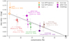Fig. 4. SNe Ia magnitude steps, γ, as a function of the tracer contamination (c = ca + cb), using the spectroscopic lsSFR as reference (cspec − lsSFR ≡ 0). The large circles are the steps derived using the SNfactory dataset (this work), while the small hexagons are the literature results (see Sect. 5). The large open (resp. full) circles are local (resp. global) measurements (see legend); the SNfactory-based and literature results have the same colors. The literature contaminations are those derived using the SNfactory sample and have been shifted by +1% for visibility. The Kelsey et al. (2021) related hexagonal markers are transparent as they measure the magnitude step after standardization, while all other data points (both with our SNfactory sample and the literature results) fit γ as a third standardization parameter (see Sect. 4.2). The full black diamond indicates the 0 mag step associated by definition with 100% contamination, corresponding to a random SN population classification. The straight black line shows our model of the measured step as a function of the contamination, linking the reference tracer point to the black diamond (see Sect. 2). The dashed gray line is a fit to the literature measurements, constrained to pass through the random classification value (black diamond).

The step amplitudes as a function of the tracer contaminations follow the expected trend given by Eq. (3), shown by the straight black line in the figure, remarkably well. As detailed in Sect. 2, this diagonal, which goes from γ₀ at c = 0% (the reference tracer step value) to 0 at c = 100% (the black diamond in the figure), is expected if two SN Ia populations exist with different mean magnitudes, and if we are using tracers that are not perfectly able to discriminate between the two populations (c > 0) to measure their magnitude offset. We note that c = 100% corresponds to randomly distributed SNe Ia between the two classes, and the expected magnitude difference between the two resulting groups is thus 0 by definition (as seen in Fig. 1).

We added to Fig. 4 the recent results from the literature with the step measurements that were made using the same techniques as the ones we used. Specifically, we added the lsSFR from Rigault et al. (2020); the local (3 kpc) U − V (similar to u − r) and global host stellar mass (split at 10¹⁰ M_⊙) from Roman et al. (2018); the local (1.5 kpc) stellar mass and photometric sSFR from Jones et al. (2018); and the morphology from Pruzhinskaya et al. (2020). We used the global host mass-step from Roman et al. (2018) for it is derived using the state-of-the-art Betoule et al. (2014) + SNLS five-year sample and the Malmquist bias correction were not made using the 5D implementation of the Beams with Bias Correction (BBC; Scolnic & Kessler 2016; Kessler & Scolnic 2017). Smith et al. (2020) showed that this implementation can bias the reported step if intrinsic SN–host correlations are not accounted for. We also used the global host mass step from Smith et al. (2020). Finally, we plotted in this figure the local (4 kpc) U − R and stellar mass from Kelsey et al. (2021) with a transparent marker, as γ is fitted after the standardization in that paper (while we fit it as a third standardization parameter, see Sect. 4.2). For these literature data points we use the reported steps while using our derived tracer contaminations. We note that if the steps are considered to be SN sample dependent (e.g., due to the light curve extraction pipeline), this implies that the contaminations are purely galaxy properties that are unrelated to the SNe Ia.

Figure 4 shows that step amplitudes measured using the SNfactory data and measured using any of the literature environmental tracers are in remarkable agreement with the corresponding independent literature measurements. For instance the Jones et al. (2018) local mass step is 0.067 ± 0.017 mag, while we measure 0.053 ± 0.031 mag and the local U − V color step from Roman et al. (2018) is 0.091 ± 0.013 mag and we find 0.096 ± 0.035 mag. The SNfactory SNe Ia data thus seem to be representative of that of the literature.

Under the assumption of multiple populations, implicitly implied by the environmental step functional form, the fact that the relationship between observed environmental step and tracer contamination is compatible with our two-populations model, for both SNfactory and the literature data points, suggests that two populations are enough to explain the observations and that both populations differ in standardized brightness by γ₀ ∼ 0.13 mag. Fitting for γ₀ using literature data points, as shown in Fig. 4, we find 0.121 ± 0.010 mag. This claim assumes that spectroscopic lsSFR is a perfect tracer. We study the use of the other tracers as the reference tracer in Sect. 6.2.

In reality, no tracer is perfect and if the spectroscopic lsSFR contamination were to be a small percentage, then γ₀ would actually be higher. For instance if c_{spec − lsSFR} = 10% and γ_{spec − lsSFR} = 0.13 mag then γ₀ = γ_{spec − lsSFR}(1 − c)⁻¹ = 0.145 mag. Consequently, the reported γ₀ measurements made in this analysis assuming we have a noisy but perfect tracer are, in fact, lower limits on the actual SN Ia population difference in magnitude means. The true spectroscopic lsSFR contamination is beyond the scope of this work.

6. Discussion

In this section we present variations to the main analysis, and then discuss the consequences of our findings. We first study the impact of fixing the stretch and color standardization coefficients to that of the reference tracer. We then change which tracer is used as a reference and compare their ability to describe the data.

6.1. Fixing α and β

In Sect. 5, we fit the standardization coefficients α, β, and γ for each environmental tracer independently to find that the two-populations model detailed in Sect. 2 seems to explain the observed variations between the tracer γ parameters. Their apparent inconsistency is due to the ability of a tracer to accurately distinguish between the two underlying populations. In that context, because the standardization coefficients are correlated, especially α and γ (see, e.g., Fig. 7 of Rigault et al. 2020), if one is not able to accurately measure γ since its environmental tracer is inaccurate, one will in turn bias the derivation of the other standardization parameters, as the fitter will use them to counterbalance the γ error.

The natural solution in the context of the two-populations model, which is implicitly assumed when doing a step analysis, is that the value of α and β must be fixed to those derived when using the reference tracer when fitting Eq. (13) for the comparison tracers. The results of this alternative and more accurate analysis is given in Table 1 (column γ*) and illustrated in the top left plot in Fig. 5. We see, comparing this plot with Fig. 4, that the results converge on the model’s expectations.

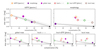Fig. 5. Similar to Fig. 4, but changing the reference tracer choice by (from left to right, top to bottom) the spectroscopic lsSFR, the host galaxy morphology, the global host galaxy stellar mass, the local u − r color, the photometric lsSFR, and the local stellar mass. In this figure the α and β have been fixed to that of the reference tracer used in each subplot (see Sect. 6.1). The gray band around the black line is the expected scatter along the diagonal (see Sect. 6.2). The more the data deviate from the model expectation (black line), the less likely it is for the reference tracer to be closely connected to the actual underlying astrophysical origin.

6.2. Testing the reference tracer

In this section, we vary which tracer is used as a reference tracer and we re-derive the resulting contamination terms, c^a and c^b, as well as the steps γ* assuming the reference’s α and β are as detailed in Sect. 6.1. If a tracer is a good reference, that is, if it can accurately discriminating between the true underlying two populations, then the other tracers should follow the diagonal line given by Eq. (3), anchored at the value of γ₀ of the reference tracer. If a reference tracer is bad, the contamination associated with this tracer does not probe the ability of a comparison tracer to discriminate between the two underlying populations. In that case the points are not expected to follow the diagonal model.

This is what we qualitatively observe in Fig. 5. Morphology is a bad reference tracer, as the other tracers lie far from its expected diagonal. This means that the morphology is not able to accurately discriminate between the two underlying populations causing the environmental steps observed by the different tracers. Conversely, the spectroscopic lsSFR, the global mass, and the local u − r colors seem to be better reference tracers.

To quantify this observation we first need to model how much scatter we should expect along the diagonal if we had access to a perfect tracer. This is mandatory since the step measurements are not independent; they all are made from the same sample of SNe Ia, but using different galaxy property indicators.

We use the simulation tool from Sect. 2 to simulate a sample with the same characteristics as the SNfactory sample, N = 110, p_a = 0.5, σ_a = σ_b = 0.1, and the γ₀ corresponding to the reference tracer step γ in Table 1. We then assume a c_a and a c_b, which define the four $N_i^j$ with i = {a, b} and j = {a, b}. We randomly shuffle the sample to follow these $N_i^j$ and we measure γ. This last step is repeated 5000 times to determine the scatter on γ caused by the randomness of which target belongs to the off-diagonal terms or not. If the two-populations model is correct, and if we measure the tracer γ parameters with a single dataset, then this scatter corresponds to the expected variations given tracer c_a and c_b parameters. The amplitude of this scatter as a function of the tracer contaminations is shown as a gray band along the model’s diagonal in Fig. 5.

Once we have determined the scatter σ(c) expected given the amount of contamination c, we can measure the χ² associated with the ability of each reference tracer to explain the data, such that

$$\begin{array}{c}\hfill {\chi }_{\mathrm{ref}}^2={\displaystyle \sum _t{\left(\frac{{\gamma }_t^{\ast }-\gamma (c_t)}{\sigma (c_t)}\right)}^2,}\end{array}$$(14)

where t refers to the comparison tracers, ${\gamma }_t^{*}$ is the fitted step value fixing α and β to those of the reference (see Sect. 6.1), and γ(c_t) is the expected step at contamination c_t following Eq. (3). Finally, since the c_t measurements are noisy, we compute the ${\chi }_{\text{ref}}^2$ for each c_t chain walkers. We report in Fig. 6 (top panel) the median ${\chi }_{\text{ref}}^2$ for each tracer used as reference together with the 16% and 84% variations. This figure also displays the individual χ² contributions (main panel).

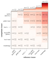Fig. 6. Matrix reporting the median χ2 for each reference tracer (columns) and each comparison tracer (rows) together with the 16% and 84% variations. The color red refers to the individual χ2 values: the darker the color, the worse the value. At the top of the matrix is plotted, for each reference tracer choice, the median with the 16% and 84% variations when summing the tracer walkers following Eq. (14).

The χ² results confirm the qualitative observations. The spectroscopic lsSFR is the optimal reference tracer, followed by the global mass, the photometric lsSFR and the local u − r colors. Local mass and morphology are the least suitable. Since the spectroscopic lsSFR is the best reference tracer choice, it means that it discriminates most accurately between the two underlying populations, which further strengthens the claim that there seems to be a prompt versus delayed age dichotomy.

Quantitatively, with χ² = 8.5 for 5 degrees of freedom, the scatter along the contamination line for spectroscopic lsSFR as the reference is consistent with random scatter of 1.1σ. The scatter for global mass as the reference has χ² = 13.6, corresponding to a scatter of 2.1σ. All other tracers are excluded from being accurate reference tracers at more than 5σ.

6.3. Scatter in the two-populations model

The two-populations model also has consequences for the observed scatter of the studied quantity q (see the introduction to the two-populations model in Sect. 2). If both populations differ by γ₀ on average in q, and keeping the assumption of 50% of the targets belonging to the a population, then we can show that marginalizing the populations results in an additional scatter in the dispersion of q by 0.5 × γ₀.

In the context of SNe Ia cosmology the studied quantity q is the standardized magnitude and interestingly the intrinsic scatter, corresponding to the part of the standardized magnitude dispersion along the Hubble diagram that cannot be explained by known sources of errors, typically is of 0.10 mag (Betoule et al. 2014; Scolnic et al. 2018).

Hence, assuming the two-populations model, if the 0.10 mag intrinsic SNe Ia scatter were fully caused by the existence of two underlying populations, the average standardized magnitude difference between these populations would be 0.2 mag. This is illustrated in the left panel of Fig. 7: in this mock example, the observed full distribution of q seems like a flattened distribution with a larger scatter than the underlying individual Gaussian distributions.

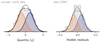Fig. 7. Illustration of the scatter in the two-populations model. Left panel: distribution of quantity q for the same mock data as in the top panel of Fig. 1, represented by the gray histogram. The full thick gray line shows the Gaussian parameters associated with this distribution. The blue and orange curves represent the estimation of the q distribution from the a and b populations, respectively, while the black curve is their sum. Right panel: distribution of the Hubble residuals of the SNfactory dataset, represented by the gray histogram. The full thick gray line shows the Gaussian that parameterizes this distribution. The dashed orange and dashed blue curves show the expected distribution of the two underlying populations that would explain the full intrinsic distributions (see Sect. 6.3). The dashed gray line is their sum and should be compared to the histogram.

If we apply this concept to the SNfactory dataset, which also has an intrinsic dispersion of ∼0.10 mag (Rigault et al. 2020), we can then guess the two underlying population distributions that would cause this effect; this is illustrated in the right panel of Fig. 7. In the case of the SNfactory standardization SNe Ia distribution, the central part (mag ∼ 0) does not seem to qualitatively follow the expected distribution. This suggests that the entire intrinsic distribution might not be fully explained by the existence of a magnitude bias of ∼0.2 mag between two underlying SN Ia populations.

Interestingly, this conceptual analysis provides key information on the upper limit of the astrophysical bias affecting SNe Ia standardized magnitudes in the context of the two populations model: it cannot be larger than twice the intrinsic dispersion and, consequently, it is smaller than ∼0.2 mag.

In addition, if the magnitude step related to the spectroscopic lsSFR is ∼0.16 mag, as claimed by Rigault et al. (2020), then the contamination of this tracer is lower than 25%.

7. Conclusion

We use a sample of 110 SNe Ia from the Nearby Supernovae Factory dataset to study the apparent inconsistencies in the literature between the different observed environmental dependencies of the standardized SNe Ia magnitudes. In the last ten years the SNe Ia luminosity has been shown to significantly depend on host properties, ranging from barely significant variations when split by host galaxy morphology (e.g., Pruzhinskaya et al. 2020) to a very significant 15% luminosity difference when the SNe are split with respect to the spectroscopic specific star formation rate of their local environment (Rigault et al. 2020), leaving the 8% luminosity difference measured using the commonly used global host galaxy mass step in between (e.g., Sullivan et al. 2010; Roman et al. 2018).

To study these variations we first analyze the mathematical implications of assuming a step function (i.e., of comparing the SN Ia magnitude means when splitting the data into two bins). We show that doing so implicitly assumes two things: (1) that there exists two underlying populations that differ in standardized magnitudes and (2) that the environmental tracer used is somewhat able to distinguish them. Exploration of the implications of this implicit two-populations model enables us to demonstrate that the expected step observed by a tracer depends on its ability to accurately discriminate between the two underlying populations. In detail, if we call c the fraction of targets misclassified by the environmental tracer, and if we call γ₀ the true difference in mean magnitudes between the two populations, then the expected measured magnitude means offset γ is given by γ = γ₀ × (1−c). The higher the contamination, hence the lower the tracer accuracy, the lower the expected measured step. In addition, the intrinsic magnitude dispersion caused by marginalizing the populations is half their magnitude offset. Since SNe Ia intrinsic dispersion is typically ∼0.10 mag, the upper limit magnitude offset between the two SNe Ia populations would be ∼0.20 mag, if the entire SNe Ia intrinsic scatter was caused by the existence of these two populations.

In light of that prediction, we derive the main literature environmental tracers for each of the 110 SNe Ia: spectroscopic and photometric measurements of the local specific star formation rate, the global and local stellar masses, the host galaxy morphology, and the local color. In this first analysis, we assume that one of these tracers is set as a reference. This provides a lower limit on the expected true amplitude of γ₀. We draw from this analysis the following conclusions.

Tracer contamination model. Our model of a “two SN Ia populations model observed with tracers of various accuracy” explains well the observed variations. In Fig. 4 we show the expected versus measured magnitude step as a function of the derived tracer contaminations and we find good agreement, which supports a two-populations model. When applied to the steps reported in the literature, our model is able to explain the observed variations.

Spectroscopic lsSFR as reference tracer. When compared to the other tracers, using the spectroscopic local specific star formation rate as a reference tracer can explain all other observations with a scatter at 1.1σ. All other measurements are excluded as suitable reference tracers, with the possible exception of global mass, which shows a 2.1σ scatter, as we can see in Fig. 5 and quantified in Fig. 6.

The prompt versus delayed model. The spectroscopic lsSFR measures the fraction of young stars in the SNe Ia vicinity. As all observations are explained by using it as the reference tracer, the prompt versus delayed progenitor age model seems to best represent the behavior of the underlying populations. Nicolas et al. (2021) further show that this model also explains the observed redshift-drift of the SN Ia stretch distribution.

Origin of the mass-step. It seems that two populations related to progenitor age, combined with tracer accuracy, can explain all previous measurements of the mass-step. This conclusion is in agreement with former analyses (e.g., Rigault et al. 2013, 2020; Roman et al. 2018).

Standardization coefficients α, β. Because the standardizing parameters such as stretch and color are correlated with the two underlying populations, hence with their tracers, the use of an inaccurate tracer, such as morphology, biases the derivation of α and β, as would a non-simultaneous estimation of α, β, and γ.

The amplitude of γ. Under the assumption of the two-populations model, the amplitude of the astrophysical bias affecting the SNe Ia luminosity (i.e., the intercept of the γ(c) plot) is close to the age-step reported in Rigault et al. (2020) (0.162 ± 0.029 mag) since the spectroscopic lsSFR is a good reference tracer. When we fit the intercept jointly on all literature data points using the derived contaminations from SNfactory sample, we find 0.121 ± 0.010 (see Fig. 4).

In light of the described two-populations model and the importance of tracer accuracy when assessing the amplitude of the astrophysical bias in SNe Ia cosmology, we highlight the importance of careful analyses of astrophysical biases when deriving cosmological parameters. This is true even when comparing two SN Ia samples at similar redshift ranges, if their selection function favored a given underlying population for any reason.

To avoid biases, one might want to probe as accurately as possible the underlying populations and to be careful when assessing them using only moderately good tracers such as global ones. In practice we urge caution with respect to current cosmological analyses that use the mass-step as the third standardization parameter to account for astrophysical dependencies in the SN Ia magnitude. The host stellar mass is not the underlying parameter affecting the SN Ia progenitor explosion mechanism; we see it, rather, as a tracer correlated with the true underlying physics. As astrophysical properties evolve significantly with cosmic time, it is critical to understand the relationship between SN Ia luminosity and the environment when doing SNe Ia cosmology.

Acknowledgments

We thank the anonymous referee for the constructive comments which helped to improve the conclusions of the paper. This project has received funding from the European Research Council (ERC) under the European Union’s Horizon 2020 research and innovation program (grant agreement n°759194 - USNAC). This work was supported in part by the Director, Office of Science, Office of High Energy Physics of the U.S. Department of Energy under Contract No. DE-AC025CH11231. Additional support was provided by NASA under the Astrophysics Data 1095 Analysis Program grant 15-ADAP15- 0256 (PI: Aldering).

References

Appendix A: Mathematical derivation of the modeling for two populations of SNe Ia

A.1. Two-populations model

The two-populations model estimates the probability of measuring certain fractions of false positives and false negatives, given known fractions of intrinsic false positives and false negatives. Closely following the notations presented in Section 2, we introduce the following variables:

• k_i = {a; b} is a discrete indicator describing the true type of target i given the two SN Ia populations;

• c_a and c_b are, respectively, fractions of intrinsic false a and false b targets;

• ${\widehat{t}}_i$ is the true tracer value for i target;

• t_i is the measurement of the tracer for i target;

• δt_i is the measurement uncertainty of the tracer for i target;

• t_cut is the cutoff value, discriminating between the two categories, for tracer t.

Within this context, the probability of measuring t_i while the target i truly belongs to b population, given c_b, is expressed by

$$\begin{array}{cc}\hfill \mathcal{P}(k_i,t_i\mid c_a,c_b)& ={\displaystyle {\int }_{-\infty }^{+\infty }\mathrm{d}{\widehat{t}}_i\int \mathrm{d}\theta \mathcal{P}(k_i,t_i,{\widehat{t}}_i,\theta \mid c_a,c_b)}\hfill \\ \hfill & ={\displaystyle {\int }_{-\infty }^{+\infty }\mathrm{d}{\widehat{t}}_i\int \mathrm{d}\theta \mathcal{P}(t_i\mid k_i,{\widehat{t}}_i,\theta ,c_a,c_b)\mathcal{P}(k_i,{\widehat{t}}_i,\theta \mid c_a,c_b)}\hfill \\ \hfill & ={\displaystyle {\int }_{-\infty }^{+\infty }\mathrm{d}{\widehat{t}}_i\int \mathrm{d}\theta \mathcal{P}(t_i\mid k_i,{\widehat{t}}_i,\theta ,c_a,c_b)\mathcal{P}({\widehat{t}}_i\mid k_i,\theta ,c_a,c_b)\mathcal{P}(k_i,\theta \mid c_a,c_b)}\hfill \\ \hfill & ={\displaystyle {\int }_{-\infty }^{+\infty }\mathrm{d}{\widehat{t}}_i\int \mathrm{d}\theta \mathcal{P}(t_i\mid k_i,{\widehat{t}}_i,\theta ,c_a,c_b)\mathcal{P}({\widehat{t}}_i\mid k_i,\theta ,c_a,c_b)\mathcal{P}(k_i\mid \theta ,c_a,c_b)\mathcal{P}(\theta \mid c_a,c_b)}\hfill \end{array}$$(A.1)

where θ captures all of the other model parameters that may exist (i.e., the nuisance parameters). The first of the four terms in the last integral is related to measurement uncertainties, the second is the tracer probability, the third is the type probability, the fourth is the probability of drawing a target of class k, and the rest is how nuisance parameters are related to c_a and c_b.

In this paper, we make the following assumptions:

1. Knowledge of ${\widehat{t}}_i$ is all that is needed to obtain t_i, so $\mathcal{P}(t_i\mid k_i,{\widehat{t}}_i,\theta ,c_a,c_b=\mathcal{P}(t_i\mid {\widehat{t}}_i)=\mathcal{N}(t_i;{\widehat{t}}_i,\delta t_i)$.

2. The unknown underlying distribution of ${\widehat{t}}_i$ only depends on the SN Ia population type k_i and the fraction of false a or false b targets, so $\mathcal{P}({\widehat{t}}_i\mid k_i=a,\theta ,c_a)=\mathcal{P}({\widehat{t}}_i\mid k_i=a,c_a)$ and $\mathcal{P}({\widehat{t}}_i\mid k_i=b,\theta ,c_b)=\mathcal{P}({\widehat{t}}_i\mid k_i=b,c_b)$.

3. Because we are only interested in knowing if a target is measured above or below a given cut, we use simple normalized top hats (𝒰) to build the t probability distribution functions, such that $\mathcal{P}({\widehat{t}}_i\mid k_i=b,c_b)=(1-c_b)\mathcal{U}(t_{\min },t_{\mathrm{cut}})+c_b\mathcal{U}(t_{\mathrm{cut}},t_{\max })$ and $\mathcal{P}({\widehat{t}}_i\mid k_i=a,c_a)=c_a\mathcal{U}(t_{\min },t_{\mathrm{cut}})+(1-c_a)\mathcal{U}(t_{\mathrm{cut}},t_{\max })$, where (t_min, t_max) corresponds to the boundaries for the parameter ${\widehat{t}}_i$, though their values do not affect the inference (we use t_cut − t_min = t_max − t_cut ≫ δt_i). The 𝒰 are normalized such that 𝒰(x; min, max) = (max − min)⁻¹ if x within min and max and 0 otherwise. We tested the impact on this hypothesis on our results by simulating many mock samples with non-top hat functions, namely Gaussians or Gaussian mixtures with various parameters. When fitting these simulations with our baseline top hat model, we accurately recover the input c_a and c_b values for a large range of c value combinations.

4. In first approximation, the fraction of true a targets is constant. Notably, this requires that the fraction does not depend on redshift. While most likely overly simplistic for the general case, this assumption seems reasonable as we are studying data within a small redshift range (0.03 < z < 0.08). This results in 𝒫(k_i = a ∣ θ, c_a) = 𝒫(k_i = a) = p_a and 𝒫(k_i = b) = (1 − p_a).

5. As a consequence of the given assumptions, there are no nuisance parameters (θ) in the model.

This way, for the case of k_i = b, equation A.1 simplifies to

$$\begin{array}{cc}\hfill \mathcal{P}(k_i=b,t_i\mid c_b)& ={\displaystyle {\int }_{-\infty }^{+\infty }\mathrm{d}{\widehat{t}}_i\int \mathrm{d}\theta \mathcal{P}(t_i\mid {\widehat{t}}_i)\mathcal{P}({\widehat{t}}_i\mid k_i,c_b)\mathcal{P}(k_i)\mathcal{P}(\theta )}\hfill \\ \hfill & =\mathcal{P}(k_i=b){\displaystyle {\int }_{-\infty }^{+\infty }\mathrm{d}{\widehat{t}}_i\mathcal{P}(t_i\mid {\widehat{t}}_i)\mathcal{P}({\widehat{t}}_i\mid k_i=b,c_b)}\hfill \\ \hfill & =(1-p_a){\displaystyle {\int }_{-\infty }^{+\infty }\mathrm{d}{\widehat{t}}_i\mathcal{N}(t_i;{\widehat{t}}_i,\delta t)((1-c_b)\mathcal{U}(t_{\min },t_{\mathrm{cut}})+c_b\mathcal{U}(t_{\mathrm{cut}},t_{\max }))}\hfill \\ \hfill & =(1-p_a){\displaystyle ({\int }_{-\infty }^{t_{\mathrm{cut}}}\mathrm{d}{\widehat{t}}_i\mathcal{N}({\widehat{t}}_i;t_i,\delta t)(1-c_b)\mathcal{U}(t_{\min },t_{\mathrm{cut}})+{\int }_{t_{\mathrm{cut}}}^{+\infty }\mathrm{d}{\widehat{t}}_i\mathcal{N}({\widehat{t}}_i;t_i,\delta t)c_b\mathcal{U}(t_{\mathrm{cut}},t_{\max }))}\hfill \\ \hfill & =\frac{1-p_a}{\mathrm{\Delta }}((1-c_b){\displaystyle {\int }_{t_{\min }}^{t_{\mathrm{cut}}}}\mathrm{d}{\widehat{t}}_i\mathcal{N}({\widehat{t}}_i;t_i,\delta t)+c_b{\displaystyle {\int }_{t_{\mathrm{cut}}}^{t_{\max }}}\mathrm{d}{\widehat{t}}_i\mathcal{N}({\widehat{t}}_i;t_i,\delta t))\hfill \\ \hfill & =\frac{1-p_a}{\mathrm{\Delta }}((1-c_b)\times f_i+c_b\times (1-f_i))\hfill \end{array}$$(A.2)

where $f_i={\int }_{t_{\min }}^{t_{\mathrm{cut}}}\mathrm{d}{\widehat{t}}_i\mathcal{N}({\widehat{t}}_i;t_i,\delta t)$ is assimilated to the cumulative distribution function (see eq. 4 in the main text) ; Δ = (t_max − t_cut) = (t_cut − t_min) is a constant normalization term.

A.2. Two-populations model with a reference tracer

Adding the reference tracer (and applying the same assumptions as above), we obtain

$$\begin{array}{cc}\hfill \mathcal{P}(k_i=b,t_i,t_i^{\mathrm{ref}}\mid c_b,c_b^{\mathrm{ref}})& ={\displaystyle {\int }_{-\infty }^{+\infty }\mathrm{d}{\widehat{t}}_i{\int }_{-\infty }^{+\infty }\mathrm{d}{\widehat{t}}_i^{\mathrm{ref}}\int \mathrm{d}\theta \mathcal{P}(k_i,t_i,{\widehat{t}}_i,t_i^{\mathrm{ref}},{\widehat{t}}_i^{\mathrm{ref}},\theta \mid c_b,c_b^{\mathrm{ref}})}\hfill \\ \hfill & ={\displaystyle {\int }_{-\infty }^{+\infty }\mathrm{d}{\widehat{t}}_i{\int }_{-\infty }^{+\infty }\mathrm{d}{\widehat{t}}_i^{\mathrm{ref}}\int \mathrm{d}\theta }\begin{array}{cc}& \mathcal{P}(t_i\mid k_i,{\widehat{t}}_i,t_i^{\mathrm{ref}},{\widehat{t}}_i^{\mathrm{ref}},\theta ,c_b,c_b^{\mathrm{ref}})\hfill \\ \times \hfill & \mathcal{P}(t_i^{\mathrm{ref}}\mid k_i,{\widehat{t}}_i,{\widehat{t}}_i^{\mathrm{ref}},\theta ,c_b,c_b^{\mathrm{ref}})\hfill \\ \times \hfill & \mathcal{P}({\widehat{t}}_i\mid k_i,{\widehat{t}}_i^{\mathrm{ref}},\theta ,c_b,c_b^{\mathrm{ref}})\hfill \\ \times \hfill & \mathcal{P}({\widehat{t}}_i^{\mathrm{ref}}\mid k_i,\theta ,c_b,c_b^{\mathrm{ref}})\hfill \\ \times \hfill & \mathcal{P}(k_i\mid \theta ,c_b,c_b^{\mathrm{ref}})\hfill \\ \times \hfill & \mathcal{P}(\theta \mid c_b,c_b^{\mathrm{ref}})\hfill \end{array}\hfill \\ \hfill & ={\displaystyle {\int }_{-\infty }^{+\infty }\mathrm{d}{\widehat{t}}_i{\int }_{-\infty }^{+\infty }\mathrm{d}{\widehat{t}}_i^{\mathrm{ref}}\int \mathrm{d}\theta \mathcal{P}(t_i\mid {\widehat{t}}_i)\mathcal{P}(t_i^{\mathrm{ref}}\mid {\widehat{t}}_i^{\mathrm{ref}})\mathcal{P}({\widehat{t}}_i\mid k_i,c_b)\mathcal{P}({\widehat{t}}_i^{\mathrm{ref}}\mid k_i,c_b^{\mathrm{ref}})\mathcal{P}(k_i)\mathcal{P}(\theta )}\hfill \\ \hfill & =\mathcal{P}(k_i=b){\displaystyle {\int }_{-\infty }^{+\infty }\mathrm{d}{\widehat{t}}_i{\int }_{-\infty }^{+\infty }\mathrm{d}{\widehat{t}}_i^{\mathrm{ref}}\mathcal{P}(t_i\mid {\widehat{t}}_i)\mathcal{P}(t_i^{\mathrm{ref}}\mid {\widehat{t}}_i^{\mathrm{ref}})\mathcal{P}({\widehat{t}}_i\mid k_i=b,c_b)\mathcal{P}({\widehat{t}}_i^{\mathrm{ref}}\mid k_i=b,c_b^{\mathrm{ref}})}\hfill \\ \hfill & =(1-p_a)\begin{array}{cc}& \times {\displaystyle {\int }_{-\infty }^{+\infty }\mathrm{d}{\widehat{t}}_i\mathcal{N}(t_i;{\widehat{t}}_i,\delta t)((1-c_b)\mathcal{U}(t_{\min },t_{\mathrm{cut}})+c_b\mathcal{U}(t_{\mathrm{cut}},t_{\max }))}\hfill \\ \hfill & \times {\displaystyle {\int }_{-\infty }^{+\infty }\mathrm{d}{\widehat{t}}_i^{\mathrm{ref}}\mathcal{N}(t_i^{\mathrm{ref}};{\widehat{t}}_i^{\mathrm{ref}},\delta t^{\mathrm{ref}})((1-c_b^{\mathrm{ref}})\mathcal{U}(t_{\min }^{\mathrm{ref}},t_{\mathrm{cut}}^{\mathrm{ref}})+c_b^{\mathrm{ref}}\mathcal{U}(t_{\mathrm{cut}}^{\mathrm{ref}},t_{\max }^{\mathrm{ref}}))}\hfill \end{array}\hfill \\ \hfill & =\frac{1-p_a}{{\mathrm{\Delta }}^{\prime }}((1-c_b)\times f_i+c_b\times (1-f_i))((1-c_b^{\mathrm{ref}})\times f_i^{\mathrm{ref}}+c_b^{\mathrm{ref}}\times (1-f_i^{\mathrm{ref}}))\hfill \end{array}$$(A.3)

Similarly for k_i = a, we get

$$\begin{array}{c}\hfill \mathcal{P}(k_i=a,t_i,t_i^{\mathrm{ref}}\mid c_a,c_a^{\mathrm{ref}})=\frac{p_a}{{\mathrm{\Delta }}^{\prime }}(c_a\times f_i+(1-c_a)\times (1-f_i))(c_a^{\mathrm{ref}}\times f_i^{\mathrm{ref}}+(1-c_a^{\mathrm{ref}})\times (1-f_i^{\mathrm{ref}}))\end{array}$$(A.4)

Finally, marginalizing over the population type, we find the general form of Eq. 10:

$$\begin{array}{cc}\hfill \mathcal{P}(t_i,t_i^{\mathrm{ref}}\mid c_a,c_b,c_a^{\mathrm{ref}},c_b^{\mathrm{ref}})& ={\displaystyle \int }\mathrm{d}{k}_i\mathcal{P}(k_i,t_i,t_i^{\mathrm{ref}}\mid c_a,c_b,c_a^{\mathrm{ref}},c_b^{\mathrm{ref}})\hfill \\ \hfill & =\mathcal{P}(k_i=a,t_i,t_i^{\mathrm{ref}}\mid c_a,c_a^{\mathrm{ref}})+\mathcal{P}(k_i=b,t_i,t_i^{\mathrm{ref}}\mid c_b,c_b^{\mathrm{ref}})\hfill \\ \hfill & \propto p_a(c_a^{\mathrm{ref}}\times f_i^{\mathrm{ref}}+(1-c_a^{\mathrm{ref}})\times (1-f_i^{\mathrm{ref}}))(c_a\times f_i+(1-c_a)\times (1-f_i))\hfill \\ \hfill & +(1-p_a)((1-c_b^{\mathrm{ref}})\times f_i^{\mathrm{ref}}+c_b^{\mathrm{ref}}\times (1-f_i^{\mathrm{ref}}))((1-c_b)\times f_i+c_b\times (1-f_i))\hfill \end{array}$$(A.5)

A.3. Testing the model robustness over the assumptions

We tested on simulations the two main assumptions made on this analysis, namely that the fraction of a class a target is a constant equal to 50% and that the probability distribution functions of the tracer values can be approximated by a combination of top hat distributions.

1. To test the impact of a fixed p_a = 50% term, we simulated many different models with varying p_a values ranging from 1 to 99%. Each time we built five different tracers with various c_a and c_b ranging from 5% to 50%, some symmetric (c_a = c_b) and some not. When fitting these simulated samples assuming our baseline model (hence with p_a = 50%) we recovered the input c_a and c_b values with no bias as long as the input p_a is within 25 − 75% ; the bias become significant (at more than 3σ) only on the extreme (p_a < 10% or p_a > 90%).

2. To test the assumption made on the tracer distribution in order to simplify the model, we built many simulations while varying the assumed distributions. We used Gaussian models or Gaussian mixture models with various parameter values to draw a perfect tracer prior to shuffling below (above) the tracer cutoff a fraction c_a (c_b) of targets to simulate the tracer’s contamination. Random noise is added next, which we did for many combinations of c_a and c_b values. When fitting these simulated samples with our baseline model, each time we recovered the input c_a and c_b values with no bias.

We hence conclude that the assumptions made in the paper to simplify the likelihood have no consequences on our results.

All Tables

All Figures

Fig. 1. Concept of tracer purity and its impact on the step measurement of an arbitrary quantity q. Top three panels: 400 mock data, 200 of category a (in blue), normally distributed over the quantity q by 𝒩(μa = 0.5, σa = 0.5), and 200 of category b (in orange) with a similar distribution 𝒩(μb = −0.5, σb = 0.5). The figure shows the mock q values as a function of the tracer values t for three different tracers. The data are classified as a or b given the tracer values if they are measured above or below tcut, respectively. The top, middle, and bottom panels show tracers with perfect, medium, and null ability to track the two categories. The right panels show the tracer estimation of the q distribution for each tracer (in gray), to be compared to the true q distribution for each category (colored dashed lines). Bottom panel: evolution of the observed step γ = μa − μb, the difference of mean q values for targets classified as a or b by the tracers, as a function of the tracer contamination c = ca + cb; the circles show each of the three simulations illustrated in the top panels, while the line shows the prediction from Eq. (3).

In the text

Fig. 2. Correlation between uniform mock reference and comparison tracers. The color indicates the true classification following the color-coding in Fig. 1: blue for a, orange for b. The right panel of each row shows the marginalized distribution of each quadrant, following the color-coding of the circles. The light histograms correspond to the off-diagonal terms: false a in light orange, false b in light blue. Top panels: perfect and noise-free tracer, i.e., without any off-diagonal points; middle panels: imperfect (ca = 15% and cb = 25%) yet noise-free tracer, the sum of its off-diagonal terms corresponds to its contamination parameters; bottom panels: perfect but noisy tracer. In this case, plain off-diagonal fractions are 11% in false a and 7.5% in false b, while both should be 0% for a perfect tracer; the likelihood estimator (Eq. (11), see Sect. 2.4), properly accounting for the fraction of off-diagonal terms caused by measurement errors, provides contamination estimates $c_a=0.5_{-0.3}^{+0.8}\%$ and $c_b=0.9_{-0.7}^{+1.3}\%$, compatible with zero.

In the text

Fig. 3. Correlation between each environmental tracer and the spectroscopic lsSFR, as mentioned in Sect. 4. The vertical gray line is the spectroscopic lsSFR cutoff, set at log(lsSFR) = − 10.82 dex. The horizontal gray lines are the other tracer cutoffs, as defined in Sect. 4. Each figure indicates the false a and false b classification quadrants. The color of the circles, which vary from orange to blue, represents the probability for a SN Ia to be in population a (blue) or b (orange) from the spectroscopic lsSFR point of view, whereas the edge color represents the same probability, but from the comparison tracer point of view. In the right column, the histograms plot the distributions in each quadrant. Orange (resp. blue) bars correspond to the truly b (resp. a) spectroscopic lsSFR classification. The estimated ca and cb parameters are given in percentages within the corresponding quadrants where the histogram is transparent.

In the text

Fig. 4. SNe Ia magnitude steps, γ, as a function of the tracer contamination (c = ca + cb), using the spectroscopic lsSFR as reference (cspec − lsSFR ≡ 0). The large circles are the steps derived using the SNfactory dataset (this work), while the small hexagons are the literature results (see Sect. 5). The large open (resp. full) circles are local (resp. global) measurements (see legend); the SNfactory-based and literature results have the same colors. The literature contaminations are those derived using the SNfactory sample and have been shifted by +1% for visibility. The Kelsey et al. (2021) related hexagonal markers are transparent as they measure the magnitude step after standardization, while all other data points (both with our SNfactory sample and the literature results) fit γ as a third standardization parameter (see Sect. 4.2). The full black diamond indicates the 0 mag step associated by definition with 100% contamination, corresponding to a random SN population classification. The straight black line shows our model of the measured step as a function of the contamination, linking the reference tracer point to the black diamond (see Sect. 2). The dashed gray line is a fit to the literature measurements, constrained to pass through the random classification value (black diamond).

In the text

Fig. 5. Similar to Fig. 4, but changing the reference tracer choice by (from left to right, top to bottom) the spectroscopic lsSFR, the host galaxy morphology, the global host galaxy stellar mass, the local u − r color, the photometric lsSFR, and the local stellar mass. In this figure the α and β have been fixed to that of the reference tracer used in each subplot (see Sect. 6.1). The gray band around the black line is the expected scatter along the diagonal (see Sect. 6.2). The more the data deviate from the model expectation (black line), the less likely it is for the reference tracer to be closely connected to the actual underlying astrophysical origin.

In the text

Fig. 6. Matrix reporting the median χ2 for each reference tracer (columns) and each comparison tracer (rows) together with the 16% and 84% variations. The color red refers to the individual χ2 values: the darker the color, the worse the value. At the top of the matrix is plotted, for each reference tracer choice, the median with the 16% and 84% variations when summing the tracer walkers following Eq. (14).

In the text

Fig. 7. Illustration of the scatter in the two-populations model. Left panel: distribution of quantity q for the same mock data as in the top panel of Fig. 1, represented by the gray histogram. The full thick gray line shows the Gaussian parameters associated with this distribution. The blue and orange curves represent the estimation of the q distribution from the a and b populations, respectively, while the black curve is their sum. Right panel: distribution of the Hubble residuals of the SNfactory dataset, represented by the gray histogram. The full thick gray line shows the Gaussian that parameterizes this distribution. The dashed orange and dashed blue curves show the expected distribution of the two underlying populations that would explain the full intrinsic distributions (see Sect. 6.3). The dashed gray line is their sum and should be compared to the histogram.

In the text

References

- Alam, S., Albareti, F. D., Allende Prieto, C., et al. 2015, ApJS, 219, 12 [Google Scholar]
- Aldering, G., Adam, G., Antilogus, P., et al. 2002, SPIE, 4836, 61 [Google Scholar]
- Aldering, G., Antilogus, P., Aragon, C., et al. 2020, RNAAS, 4, 63 [NASA ADS] [Google Scholar]
- Arnouts, S., & Ilbert, O. 2011, Astrophysics Source Code Library [record ascl:1108.009] [Google Scholar]
- Arnouts, S., Cristiani, S., Moscardini, L., et al. 1999, MNRAS, 310, 540 [Google Scholar]
- Aubourg, É., Tojeiro, R., Jimenez, R., et al. 2008, A&A, 492, 631 [NASA ADS] [CrossRef] [EDP Sciences] [Google Scholar]
- Banerji, M., Lahav, O., Lintott, C. J., et al. 2010, MNRAS, 406, 342 [Google Scholar]
- Barbary, K. 2016, J. Open Source Software, 1, 6 [Google Scholar]
- Betoule, M., Kessler, R., Guy, J., et al. 2014, A&A, 568, A22 [NASA ADS] [CrossRef] [EDP Sciences] [Google Scholar]
- Bolzonella, M., Miralles, J.-M., & Pelló, R. 2000, A&A, 363, 476 [Google Scholar]
- Brout, D., & Scolnic, D. 2021, ApJ, 909, 26 [NASA ADS] [CrossRef] [Google Scholar]
- Bruzual, G., & Charlot, S. 2003, MNRAS, 344, 1000 [NASA ADS] [CrossRef] [Google Scholar]
- Calzetti, D. 2013, Secular Evolution of Galaxies, 419 [CrossRef] [Google Scholar]
- Casado, J., Ascasibar, Y., Gavilán, M., et al. 2015, MNRAS, 451, 888 [NASA ADS] [CrossRef] [Google Scholar]
- Chambers, K. C., Magnier, E. A., Metcalfe, N., et al. 2016, ArXiv e-prints [arXiv:1612.05560] [Google Scholar]
- Childress, M., Aldering, G., Antilogus, P., et al. 2013a, ApJ, 770, 108 [Google Scholar]
- Childress, M., Aldering, G., Antilogus, P., et al. 2013b, ApJ, 770, 107 [NASA ADS] [CrossRef] [Google Scholar]
- Choi, Y.-Y., Han, D.-H., & Kim, S. S. 2010, J. Korean Astron. Soc., 43, 191 [NASA ADS] [CrossRef] [Google Scholar]
- Dixon, S. 2021, PASP, 133, 054501 [NASA ADS] [CrossRef] [Google Scholar]
- Fitzpatrick, E. L. 1999, PASP, 111, 63 [Google Scholar]
- Foreman-Mackey, D., Hogg, D. W., Lang, D., et al. 2013, PASP, 125, 306 [NASA ADS] [CrossRef] [Google Scholar]
- Freedman, W. L., Madore, B. F., Gibson, B. K., et al. 2001, ApJ, 553, 47 [Google Scholar]
- Freedman, W. L., Madore, B. F., Hatt, D., et al. 2019, ApJ, 882, 34 [Google Scholar]
- Gupta, R. R., D’Andrea, C. B., Sako, M., et al. 2011, ApJ, 740, 92 [Google Scholar]
- Gupta, R. R., Kuhlmann, S., Kovacs, E., et al. 2016, AJ, 152, 154 [NASA ADS] [CrossRef] [Google Scholar]
- Henne, V., Pruzhinskaya, M. V., Rosnet, P., et al. 2017, New Astron., 51, 43 [CrossRef] [Google Scholar]
- Ilbert, O., Arnouts, S., McCracken, H. J., et al. 2006, A&A, 457, 841 [NASA ADS] [CrossRef] [EDP Sciences] [Google Scholar]
- Jones, D. O., Riess, A. G., & Scolnic, D. M. 2015, ApJ, 812, 31 [NASA ADS] [CrossRef] [Google Scholar]
- Jones, D. O., Riess, A. G., Scolnic, D. M., et al. 2018, ApJ, 867, 108 [NASA ADS] [CrossRef] [Google Scholar]
- Karman, W., Caputi, K. I., Caminha, G. B., et al. 2017, A&A, 599, A28 [NASA ADS] [CrossRef] [EDP Sciences] [Google Scholar]
- Kauffmann, G., Heckman, T. M., White, S. D. M., et al. 2003, MNRAS, 341, 54 [Google Scholar]
- Kelly, P. L., Hicken, M., Burke, D. L., et al. 2010, ApJ, 715, 743 [Google Scholar]
- Kelsey, L., Sullivan, M., Smith, M., et al. 2021, MNRAS, 501, 4861 [NASA ADS] [CrossRef] [Google Scholar]
- Kennicutt, R. 1998, LIA Colloq. 34: The Next Generation Space Telescope: Science Drivers and Technological Challenges, 429, 81 [NASA ADS] [Google Scholar]
- Kessler, R., & Scolnic, D. 2017, ApJ, 836, 56 [Google Scholar]
- Kim, Y.-L., Smith, M., Sullivan, M., et al. 2018, ApJ, 854, 24 [Google Scholar]
- Kim, Y.-L., Kang, Y., & Lee, Y.-W. 2019, J. Korean Astron. Soc., 52, 181 [Google Scholar]
- Knox, L., & Millea, M. 2020, Phys. Rev. D, 101, 043533 [Google Scholar]
- Labbé, I., Oesch, P. A., Bouwens, R. J., et al. 2013, ApJ, 777, L19 [CrossRef] [Google Scholar]
- Lampeitl, H., Smith, M., Nichol, R. C., et al. 2010, ApJ, 722, 566 [Google Scholar]
- Mannucci, F., Della Valle, M., Panagia, N., et al. 2005, A&A, 433, 807 [NASA ADS] [CrossRef] [EDP Sciences] [Google Scholar]
- Mannucci, F., Della Valle, M., & Panagia, N. 2006, MNRAS, 370, 773 [Google Scholar]
- Maoz, D., Mannucci, F., & Nelemans, G. 2014, ARA&A, 52, 107 [Google Scholar]
- Nicolas, N., Rigault, M., Copin, Y., et al. 2021, A&A, 649, A74 [NASA ADS] [CrossRef] [EDP Sciences] [Google Scholar]
- Perlmutter, S., Aldering, G., Goldhaber, G., et al. 1999, ApJ, 517, 565 [Google Scholar]
- Planck Collaboration XIII. 2016, A&A, 594, A13 [NASA ADS] [CrossRef] [EDP Sciences] [Google Scholar]
- Planck Collaboration VI. 2020, A&A, 641, A6 [NASA ADS] [CrossRef] [EDP Sciences] [Google Scholar]
- Ponder, K. A., Wood-Vasey, W. M., Weyant, A., et al. 2020, ApJ, submitted, [arXiv:2006.13803] [Google Scholar]
- Pruzhinskaya, M. V., Novinskaya, A. K., Pauna, N., et al. 2020, MNRAS, 499, 5121 [NASA ADS] [CrossRef] [Google Scholar]
- Reid, M. J., Pesce, D. W., & Riess, A. G. 2019, ApJ, 886, L27 [Google Scholar]
- Riess, A. G., Filippenko, A. V., Challis, P., et al. 1998, AJ, 116, 1009 [Google Scholar]
- Riess, A. G., Macri, L., Casertano, S., et al. 2009, ApJ, 699, 539 [Google Scholar]
- Riess, A. G., Macri, L. M., Hoffmann, S. L., et al. 2016, ApJ, 826, 56 [Google Scholar]
- Riess, A. G., Casertano, S., Yuan, W., et al. 2019, ApJ, 876, 85 [Google Scholar]
- Rigault, M., Copin, Y., Aldering, G., et al. 2013, A&A, 560, A66 [NASA ADS] [CrossRef] [EDP Sciences] [Google Scholar]
- Rigault, M., Aldering, G., Kowalski, M., et al. 2015, ApJ, 802, 20 [Google Scholar]
- Rigault, M., Brinnel, V., Aldering, G., et al. 2020, A&A, 644, A176 [NASA ADS] [CrossRef] [EDP Sciences] [Google Scholar]
- Rodney, S. A., Riess, A. G., Strolger, L.-G., et al. 2014, AJ, 148, 13 [Google Scholar]
- Roman, M., Hardin, D., Betoule, M., et al. 2018, A&A, 615, A68 [NASA ADS] [CrossRef] [EDP Sciences] [Google Scholar]
- Scannapieco, E., & Bildsten, L. 2005, ApJ, 629, L85 [Google Scholar]
- Schlegel, D. J., Finkbeiner, D. P., & Davis, M. 1998, ApJ, 500, 525 [Google Scholar]
- Scolnic, D., & Kessler, R. 2016, ApJ, 822, L35 [Google Scholar]
- Scolnic, D. M., Jones, D. O., Rest, A., et al. 2018, ApJ, 859, 101 [NASA ADS] [CrossRef] [Google Scholar]
- Scolnic, D., Perlmutter, S., Aldering, G., et al. 2019, Astro 2020: Decadal Survey on Astronomy and Astrophysics, 2020, 270 [Google Scholar]
- Shimasaku, K., Fukugita, M., Doi, M., et al. 2001, AJ, 122, 1238 [NASA ADS] [CrossRef] [Google Scholar]
- Smith, M., Nichol, R. C., Dilday, B., et al. 2012, ApJ, 755, 61 [Google Scholar]
- Smith, M., Sullivan, M., Wiseman, P., et al. 2020, MNRAS, 494, 4426 [Google Scholar]
- Strateva, I., Ivezić, Ž., Knapp, G. R., et al. 2001, AJ, 122, 1861 [CrossRef] [Google Scholar]
- Sullivan, M., Le Borgne, D., Pritchet, C. J., et al. 2006, ApJ, 648, 868 [NASA ADS] [CrossRef] [Google Scholar]
- Sullivan, M., Conley, A., Howell, D. A., et al. 2010, MNRAS, 406, 782 [NASA ADS] [Google Scholar]
- Taylor, E. N., Hopkins, A. M., Baldry, I. K., et al. 2011, MNRAS, 418, 1587 [Google Scholar]
- Uddin, S. A., Mould, J., Lidman, C., et al. 2017, ApJ, 848, 56 [CrossRef] [Google Scholar]
- Wiseman, P., Sullivan, M., Smith, M., et al. 2021, MNRAS, 506, 3330 [NASA ADS] [Google Scholar]
- Wong, K. C., Suyu, S. H., Chen, G. C.-F., et al. 2020, MNRAS, 498, 1420 [Google Scholar]
- Yoshikawa, T., Akiyama, M., Kajisawa, M., et al. 2010, ApJ, 718, 112 [NASA ADS] [CrossRef] [Google Scholar]