| Issue |
A&A
Volume 657, January 2022
|
|
|---|---|---|
| Article Number | A14 | |
| Number of page(s) | 12 | |
| Section | The Sun and the Heliosphere | |
| DOI | https://doi.org/10.1051/0004-6361/202141005 | |
| Published online | 21 December 2021 | |
Heliospheric effects caused by Sun-originating versus LISM-advected fluctuations
Space Research Centre PAS (CBK PAN), Bartycka 18a, 00-716 Warsaw, Poland
e-mail: maro@cbk.waw.pl
Received:
6
April
2021
Accepted:
13
September
2021
Context. We investigate the response of the heliosphere to fluctuations in the local interstellar medium (LISM) as compared to the influence of solar-cycle fluctuations.
Aims. We discuss the differences between effects coming from the two types of drivers of time-dependent effects in the heliosphere in the context of the shape of the heliosphere, the thickness of the inner heliosheath, and the position of the ribbon of enhanced energetic neutral particle emission, as observed by the IBEX mission.
Methods. Our study is based on a comparison of fully time-dependent simulations obtained with a three-dimensional (3D) model of the heliosphere.
Results. We show that density fluctuations, taking the form of entropy waves and originating from the LISM, may reduce the thickness of the inner heliosheath to a similar extent as the solar-cycle effects. However, the relative motions of the termination shock and the heliopause in the two types of simulations are different. The amplitude of variation of the heliopause position is greater for the LISM fluctuation. The IBEX ribbon position is shown to be not significantly affected by the two types of drivers, although the effect of LISM fluctuation is stronger than that of the solar cycle. In this context, slight systematic changes of the position of the IBEX ribbon in its different sectors (i.e., changes in the heliospheric nose followed by variations in the heliospheric flanks) may serve as an indicator of the passage of a density fluctuation in the LISM, as suggested by our study. We also discuss the difficulties in fitting the LISM parameters in the presence of time-dependent effects.
Key words: Sun: heliosphere / solar wind / interplanetary medium
© ESO 2021
1. Introduction
The interaction of the solar wind (SW) with the local interstellar medium (LISM) leads to the formation of the heliosphere – a cavity in the LISM filled with plasma of solar origin. The physics of the interaction is very complex, characterized by the appearance of multiple discontinuities and various regions at the SW-LISM interface. The separatrix between SW and LISM is called the heliopause (HP), which is located between the termination shock in SW and possibly a bow shock (BS) in the interstellar medium. The inner heliosheath (IHS) is a region between the TS and HP. The outer heliosheath (OHS) is defined as located between the HP and BS, if the BS exists. Even in the absence of the BS, at some distance from the HP, the interstellar material begins to experience an obstacle in the form of the HP. This region, where the interstellar matter slows down and increases in density, is understood as the OHS. Recent studies and observations suggest that the HP should be considered, rather, as a complex interaction region than a simple laminar discontinuity (Burlaga et al. 2013; Stone et al. 2013). The complexity of the HP can be explained if localized spots of magnetic reconnection are possibly involved (Strumik et al. 2013, 2014; Swisdak et al. 2013) or plasma and plasma-neutrals instabilities are taken into account (Borovikov et al. 2008; Pogorelov et al. 2017). It has also been proposed that the HP complexity can be related to a magnetic-flux-tube interchange instability at the HP (Krimigis et al. 2013; Florinski 2015).
The heliosphere configuration is known to be determined by a variety of factors, including the relative pressures of the solar wind and the interstellar material, magnetic fields around the Sun and in the LISM, and by the interstellar ionization processes due to the influence of penetrating neutrals on the heliosphere. A substantial amount of work has been done with regard to investigating the influence of time-changing solar wind parameters on the heliosphere, including solar-cycle effects (see, e.g., Scherer & Fahr 2003; Zank & Müller 2003; Izmodenov et al. 2008; Pogorelov et al. 2017 and references therein). However, relatively little attention has been paid so far to the consideration of heliospheric configurations resulting from variations in the parameters of the LISM. The variations could be related to the impact of less or more distant supernovae blast wave or ejecta, instabilities in the interstellar medium, or possibly to the evolving Loop I superbubble that the Sun is traveling through (Müller et al. 2009; Frisch & Dwarkadas 2018). We can expect that the LISM parameters changing over time should have a direct impact on the configuration of the heliosphere. In this paper, we consider such scenarios and discuss possible heliosphere configurations under the influence of time-varying LISM parameters. We investigate the response of the heliosphere to LISM fluctuations in comparison with (and in contrast to) the influence of solar-cycle fluctuations.
The interaction of the heliosphere with LISM fluctuations is rather poorly understood. The only study involving direct time-dependent numerical simulations that we are aware of was performed by Pogorelov (2000). This early work presents results obtained from a hydrodynamic, axisymmetric model of the heliosphere, where the interstellar and solar-wind magnetic fields have not been included. According to the description presented by Pogorelov (2000), the model used in this work also disregards neutral particles at all. Periodic variations of the LISM density were included in the model and density variations in the modeled problem were discussed with some general comments on instabilities appearing at the heliopause. Based on the current state of knowledge, it is obviously important to include the magnetic field as it is known to affect the total pressure balance between the solar wind and the LISM. The magnetic field is also known to stabilize many hydrodynamic instabilities. In addition, it is clear that the effects of neutral particles should be also included. All these factors are included in our approach since we use a model where the solar wind and the interstellar medium are both magnetized and neutral particles are modeled within a constant-hydrogen-flux approximation.
In terms of the investigated heliospheric features, we focus on the size of the heliosphere parametrized by the distance to the heliopause. We also investigate the position in the sky of the IBEX ribbon – a region of enhanced emission of energetic neutral atoms (McComas et al. 2009; Funsten et al. 2009; Schwadron et al. 2009). If it is modeled as generated in the OHS beyond the HP, the IBEX ribbon carries information about the orientation of the magnetic field in the OHS, as influenced by draping effects in the proximity of the HP. We focus here on the perpendicularity condition between the line of sight and the magnetic field beyond the HP, thus, we do not consider questions related to other mechanisms needed for generation of the IBEX ribbon, such as the rate of pitch angle scattering (Chalov et al. 2010; Heerikhuisen et al. 2010; Florinski et al. 2010) or the spatial retention of pick-up protons (Schwadron & McComas 2013; Zirnstein et al. 2019).
The paper is organized as follows. In Sect. 2, we present a parametric study of heliospheric stationary solutions using sets of boundary conditions proposed by Zirnstein et al. (2016). This part of our study allows us to find the proper initial condition for our time-dependent simulations. It also makes it possible to quantify differences between solutions obtained with our constant-hydrogen-flux model and the fully-kinetic modeling of neutrals performed by Zirnstein et al. (2016). In Sect. 3, we present the results of our modeling of time-dependent effects, including the influence of the solar cycle and the LISM fluctuation on the heliosphere. The results are discussed and our conclusions are given in Sect. 4.
2. Stationary solutions
A recent paper by Zirnstein et al. (2016) provides a systematic parametric study of simulations of the heliosphere in the context of Voyager 1 measurements of the distance to the HP and observations of the IBEX ribbon – a region in the sky of the enhanced emission of energetic neutral atoms. In the first step, we analyzed simulation results obtained with our constant-hydrogen-flux model for boundary conditions proposed by Zirnstein et al. (2016), where a kinetic approach was used to simulate the neutral H component. The goal of this section is to determine differences introduced by the simplified modeling of the neutral component in our simulations.
2.1. Simulation method
We used a three dimensional (3D) Magnetohydrodynamic (MHD) model of the interaction between the SW and LISM, as described by Ratkiewicz et al. (2008), where a number of revisions have been introduced, including: a magnetized SW, boundary conditions adjusted to simulate solar cycle effects, and an improved modeling of the neutral hydrogen within the constant-flux approximation. The MHD equations are solved on a radially symmetric grid with 101 × 201 points for the polar and azimuthal angles, where the polar axis is oriented along the direction of the LISM flow. The grid points are logarithmically spaced in the radial direction, with 147 grid points extending from 10 to 5000 AU from the Sun. Therefore, the resolution in the radial direction varies from ∼0.45 AU at ∼10 AU from the Sun, through ∼2.4 AU at ∼60 AU (approximately at the modeled TS), ∼5 AU at ∼120 AU (approximately at the HP location in the heliospheric-nose direction), till ∼200 AU at ∼5000 AU. The interplanetary magnetic field is set at the inner boundary (i.e., at 10 AU from the Sun), according to the Parker model as an Archimedean spiral with a tilt of 7.25 deg between the magnetic axis and normal to the ecliptic plane. The interplanetary magnetic field is unipolar, thus, the model does not include the heliospheric current sheet. Due to a relatively sparse grid used in the model, the development of instabilities related to the magnetic reconnection between the interplanetary and interstellar magnetic field is suppressed by the diffusion of the numerical scheme. The divergence-free magnetic field is maintained using a divergence-cleaning method with an additional source term in the MHD equations, as discussed by Ratkiewicz et al. (2008). In general, both stationary and time-dependent numerical simulations can be performed using the heliospheric model.
In terms of the treatment of neutral atoms, the constant-flux approximation used in this paper can be considered as an infinite-mean-free-path limit relative to kinetic modeling. The spatial distributions of the density, velocity, and temperature for neutrals are assumed to be constant throughout the heliosphere. It is important to note that with regard to the cross-section for the charge exchange between plasma and neutrals, it is not assumed to be constant in our model. Although the velocity of the neutrals is assumed to be constant, the relative velocity of plasma and neutrals also involves the plasma velocity, which is self-consistently computed in our model and used in the estimation of the cross-section. Consequently, the cross-section is used in computations of the collision frequency between neutral atoms and protons, which affects the plasma velocity evolution via the source terms in our MHD equations. More details can be found in Eq. (1) and the discussion in Ratkiewicz et al. (2008).
Stationary solutions are obtained by using the constant-hydrogen-flux model together with boundary conditions proposed by Zirnstein et al. (2016), where a kinetic model of neutral hydrogen was shown to aptly reproduce the distance from the Sun to the HP for the Voyager 1 measurement and the position in the sky of the IBEX ribbon. Outer boundary conditions (located at 5000 AU from the Sun) in our computations are set exactly to the same values as listed by Zirnstein et al. (2016) in their Table 1. The simulated cases represent six different sets of boundary conditions that can be parametrized based on the values of the magnetic field strength, but other parameters of the LISM also vary in accordance with the magnetic field. The values of the LISM parameters are summarized in Table 1. The interstellar magnetic field direction changes depending on the magnetic field strength but remains in so-called hydrogen deflection plane defined by the interstellar He and H inflow directions (Lallement et al. 2010). The velocity of the LISM flow v∞ is set to 25.4 km s−1, its temperature is 7500 K, and the LISM flow direction is (255.7, 5.1) deg in the ecliptic frame. Inner boundary conditions at 10 AU are also set consistently with those used by Zirnstein et al. (2016). The conditions are obtained by adiabatic radial expansion of the following SW conditions at 1 AU: the density 5.74 cm−3, the temperature 51 100 K, the radial SW velocity 450 km s−1, the radial component of the magnetic field 3.75 nT. Setting the inner and outer boundary conditions exactly to the values proposed by Zirnstein et al. (2016) gives us a proper basis for a direct comparison of the kinetic-neutrals modeling results with our constant-hydrogen-flux model, where we can determine differences introduced by the simplified modeling of neutrals.
LISM parameter values.
2.2. Simulated Sun-heliopause distance
To determine the distance from the Sun to the HP in simulations, it is necessary to precisely define the HP. The plasma density is expected to jump at the HP, but in simulations, the HP is typically not a perfect discontinuity, and the jump is, in fact, a continuous transition extending over a certain number of simulation cells. In the analysis of Zirnstein et al. (2016), the HP definition was based on the presence of a “knee” in the radial profile of the plasma density. The “knee” is a break point, where a fast increase of the density is changing to a slower rate further from the Sun (priv. comm. from E. Zirnstein). In our simulations, such behavior (i.e., the presence of the “knee”) was not observed, but the definition used by Zirnstein et al. (2016) is presumably equivalent to the location of the local maximum of the slope in a plasma density profile along a line going from the OHS to IHS (e.g., along a spacecraft trajectory). We adopt such a definition for the HP in our paper and we subsequently refer to it as the HP1 definition. Another possible definition of the HP can be based on the location of a point in the plasma density profile, where the density, np = np∞, in the transition from the IHS to the OHS. This point can be determined for the upwind hemisphere due to the presence of a plasma pileup in the OHS, where the density is higher than the LISM value, namely, np > np∞. We refer to this as the HP2 definition. We use the two definitions of the HP to verify whether our findings are sensitive to a particular way of defining the HP.
Figure 1 shows the simulated density profile along Voyager 1 and 2 trajectories for the case B∞ = 0.3 nT from Table 1. Two density-based definitions HP1 and HP2 of the heliopause are shown together with a definition HP SEP based on the separatrix between the heliospheric and LISM flows. The HP-SEP-based heliopause is shifted closer to the Sun and more towards the middle part of the density jump associated with the heliopause. The two density-based definitions, HP1 and HP2, provide locations that are shifted outward with respect to HP SEP, with relatively small differences between them.
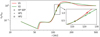 |
Fig. 1. Simulated density profile along Voyager 1 and 2 trajectories for the case where B∞ = 0.3 nT. Locations of three HP definitions are shown in the plot: HP1 (based on the maximum slope of the density profile), HP2 (isocontour np = np∞) and separatrix-based definition HP SEP. The inset shows in detail the region embraced by dashed lines in the main plot. The main plot uses the logarithmic vertical scale, while in the inset, the vertical scale is linear. |
Figure 2 shows a comparison of the two heliopause definitions (HP1 and HP2) with a streamline-based definition of the separatrix (HP SEP) between the heliospheric and LISM flows. The plot shows simulation results for the case B∞ = 0.3 nT from Table 1. The heliopause definition HP1 gives locations that are systematically shifted ∼8 − 16 AU outward from the Sun relative to the separatrix HP SEP, except for the heliotail region, where HP1 may be located closer to the Sun than the HP SEP. In the proximity of the heliospheric nose, the definitions HP1 and HP2 give very similar results, but strong differences are visible at heliospheric flanks. In terms of similarity to the separatrix-based definition, the definition HP1 seems to be superior relative to HP2. However, the definition HP2 can be also interesting from practical point of view, since it is based on a constant-density threshold. Therefore, the definition HP2 is presumably the easiest one to be implemented in analysis of data from spaceborne instruments. Although the definition HP2 is based on the LISM plasma density, np∞, that can be only roughly estimated at present, but we can expect that this definition well illustrates the behavior of entire group of density isocontours that are based on a constant density value of a similar order of magnitude as np∞.
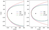 |
Fig. 2. Shape of the HP according to three different definitions for a stationary solution for the LISM magnetic field strength B∞ = 0.3 nT. Definitions HP1 and HP2 are based on the density profile and the definition HP SEP is the separatrix between the heliospheric and LISM flows computed from streamline analysis. Both the B − V-plane cut (on the left) and the perpendicular-plane cut (on the right) through the three-dimensional solution are shown. |
We might expect that a formal definition of the HP should be based on a separatrix between the solar wind and the LISM flow. However such definition is convenient only for stationary numerical solutions, because in time-dependent modeling the flow and its stagnation points become more complicated. However, the main problem is that this separatrix-based definition is completely useless from the point of view of spacecraft measurements, since spacecraft are not able to track flow lines. Based on recent crossings of the HP by Voyager 1 and 2, it is also currently not clear how discontinuities in energetic-particle fluxes are related to the magnetic-field and velocity-field separatrices for the heliosphere-LISM interaction. Therefore, the separatrix location cannot be inferred from the energetic-particle fluxes as well. For these reasons, we find the density-profile-based definitions of the HP more useful for the purposes of our study. A similar approach was adopted, for instance, by Zirnstein et al. (2016).
Figure 3 shows the simulated distance to the HP along the Voyager 1 and 2 trajectories for different sets of boundary conditions described in Sect. 2.1. For these boundary conditions, the kinetic model used by Zirnstein et al. (2016) was reported to generate solutions, where the HP was located at ∼122 AU from the Sun along the Voyager 1 trajectory. As we argue above, in our understanding, the HP1 definition is the most appropriate for direct comparison of our results with those reported by Zirnstein et al. (2016). For the HP1 definition, the distance is ∼123 AU for B∞ = 0.3 nT, but this is also dependent on the magnetic field strength; it increases from ∼116.2 to ∼127.8 AU in correlation with the magnetic field strength, which gives the maximum relative difference of the order of ∼4.7% with respect to the kinetic model for the LISM magnetic field strength values between 0.2 and 0.4 nT.
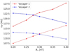 |
Fig. 3. Distance to the HP along the Voyager 1 (red) and 2 (blue) trajectories for different boundary conditions of the simulation parametrized by the strength of the unperturbed LISM magnetic field. The solid lines show the heliopause location according to the HP1 definition, while dashed lines show the location of the separatrix resulting from streamline analysis. |
The distance to the HP along the Voyager 2 trajectory was not considered by Zirnstein et al. (2016), because the spacecraft crossed the HP later, in November 2018 (Burlaga et al. 2019; Gurnett & Kurth 2019; Richardson et al. 2019). In our simulations, using the HP1 definition, this distance is anti-correlated with the magnetic field strength and varies between 117.8 and 122.8 AU (see Fig. 3, blue solid line). For B∞ = 0.3 nT, the simulated distance of ∼121 AU is slightly smaller than for Voyager 1. We should also note that the obtained distances to HP are in reasonable agreement with Voyager spacecraft measurements, 122 and 119 AU, correspondingly for Voyager 1 and 2 (Burlaga et al. 2013, 2019; Stone et al. 2013; Richardson et al. 2019).
Figure 3 shows also a comparison of the HP1 definition (solid lines) with the separatrix (dashed lines) for the heliospheric and LISM flows. The separatrix seem to be systematically shifted towards the Sun by ∼10 AU, but it behaves similarly to HP1 in its dependence on the magnetic field strength. The separatrix is commonly considered as the true heliopause resulting from hydrodynamic component of stationary MHD solutions. However, as we argued above, the separatrix-based definition of the heliopause is difficult to apply in analysis of time-dependent solutions. It is also difficult (if possible at all) to apply it in an analysis of spaceborne-instrument data, where density-based definitions can be more easily implemented.
2.3. Simulated IBEX ribbon position
Zirnstein et al. (2016) used a state-of-the-art model for computations of the energetic-neutral-atom (ENA) fluxes from the OHS based on proper calculations of the probabilities of charge-exchange between plasma and neutrals. The study confirmed that (in addition to other factors modulating the ENA flux along and across the IBEX ribbon) the perpendicularity condition  is crucial for determining the position of the ribbon in the sky, where
  is the local magnetic field unit vector in the OHS and
  represents the viewing direction unit vector (McComas et al. 2009; Funsten et al. 2009; Schwadron et al. 2009; Heerikhuisen et al. 2010).
We consider the perpendicularity condition in the ribbon-center frame as observed by the IBEX satellite, where we adopt (l, b) = (218.33, 40.38) deg in J2000 ecliptic coordinates as representing the weighted mean center of the ribbon over all energies and all years found by Dayeh et al. (2019). In Fig. 4, the polar angle θ measures the distance from the direction (l, b) = (218.33, 40.38) deg and the azimuthal angle is measured from the LISM inflow (heliospheric nose) direction. In the ribbon-center frame, the circularity and centering of the simulated perpendicularity condition can be investigated and conveniently compared with the IBEX observations, as discussed by (Funsten et al. 2009, 2013; Dayeh et al. 2019). In our analysis, the distribution of  is computed for a set of azimuthal angles, for which the observed IBEX ribbon position was provided by Funsten et al. (2013).
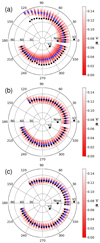 |
Fig. 4. Distributions of the simulated perpendicularity condition in the IBEX-ribbon-center frame. Black circles show the position of the observed IBEX ribbon, shades of red color-coded values of the simulated distribution of |


A comparison of the three panels in Fig. 4 shows that the perpendicularity condition moves in the sky when we change the distance from the HP. In fact, similar effects occur when the LISM magnetic field is being changed (Strumik et al. 2011; Ratkiewicz et al. 2012; Zirnstein et al. 2016). We can define an average angular distance between the condition  and the ridge of the observed IBEX ribbon as:
where N = 48 is the number of points along the ribbon for which the observed IBEX ribbon position was provided by Funsten et al. (2013) (i.e., the number of black circles in Fig. 4), θi is the polar angle of the minimum of the simulated distribution of the perpendicularity condition, and  is the polar angle of the ridge of the observed IBEX ribbon. In other words, Eq. (1) measures the average angular distance in the polar-angle coordinate θ between blue and black circles in Fig. 4.
The observed IBEX ribbon to which our simulations are compared to, is a composite of three energy passbands 0.7, 1.1, 1.7 keV as presented by Funsten et al. (2013) in their Fig. 2d. For these energies, the ribbon is a relatively narrow and well defined feature in the sky, with its angular radius weakly dependent on the energy. Additionally, since the energy composite is used in our analysis, the resulting ribbon represents an averaged structure. Such an averaged structure seems to be the most appropriate case for the comparison with the perpendicularity condition as performed in our work.
Figure 5a shows how |Δθ| changes as a function of the distance from the HP (HP1 definition used here) for different sets of boundary conditions parametrized by the LISM magnetic field strength values. In each profile, the minimum of the angular distance (thus, the best fit) occurs for the distance from the HP of ∼30 − 50 AU. The minimum minimorum is obtained for r − rHP = 50 AU and B∞ = 0.3 nT. In Fig. 4b, we can see what the best-fit simulation case looks like in greater detail on the sky map. The character of the discrepancies between the simulations and observations depending on the distance from the HP is illustrated in panels a and c of Fig. 4. Furthermore, Fig. 5b shows how the minimum in each profile from Fig. 5a depends on the LISM magnetic field strength. The case with the LISM magnetic field B∞ = 0.3 nT provides the best fit of the simulated perpendicularity condition to the observed IBEX ribbon position in the sky. We note that this estimation is close to the best-fit value of 0.293 nT obtained via similar procedure by Zirnstein et al. (2016).
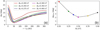 |
Fig. 5. Dependence on the distance from the HP (HP1 definition) of the average angular distance |Δθ| between the simulated perpendicularity condition and the observed IBEX ribbon for different LISM magnetic field strengths, shown in panel a. Panel b: how the minimum of each profile in panel a depends on the LISM magnetic field strength. Colors of circles in panel b correspond to colors of lines in panel a. The minimum of the simulated dependence shown in panel b gives an estimate of the LISM magnetic field strength that provides the best fit to IBEX ribbon observations. |
A similar analysis as in Fig. 5 is presented in Fig. 6 but for the definition HP2 instead of HP1. The minimum of the dependence of |Δθ|min on the LISM magnetic field strength is obtained at B∞ = 0.3 nT for the HP2 definition of the HP, similarly to the HP1 case. This suggests that the results presented in this section do not depend on a specific way of defining the HP.
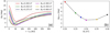 |
Fig. 6. Similar dependence as presented in Fig. 5 but for the HP2 definition of the heliopause. The dependence of |Δθ| on the distance from the HP (HP2 definition) is shown in panel a. Panel b: how the minimum of each profile in panel a depends on the LISM magnetic field strength. |
3. Time-dependent simulations
An initial setup for time-dependent simulations is adopted from the stationary case for B∞ = 0.3 nT, since the case has been found as providing the best fit to Voyagers and IBEX observations among the cases considered in our paper. As shown in the previous section, for B∞ = 0.3 nT the simulated HP in the stationary solution is located at 123 AU along the Voyager 1 trajectory and 121 AU along the Voyager 2 trajectory, which is in a reasonable agreement with the measured values, namely: 122 and 119 AU, respectively (Burlaga et al. 2013, 2019; Stone et al. 2013; Richardson et al. 2019). The value of the LISM magnetic field strength B∞ = 0.3 nT is also found in our study as providing the best fit of the simulated B ⋅ r ≈ 0 condition to the position of the IBEX ribbon in the sky.
3.1. Solar-cycle effects – method description
In the simulation that accounts for solar-cycle effects, we used the same numerical model of the heliosphere described in Sect. 2.1. The computations in the model are inherently time-dependent, thus, in the procedure of obtaining stationary solutions, simulation runs were performed on a sufficiently large time scale to converge to steady states. In contrast, in the time-dependent case with solar-cycle effects, simulations start from the stationary solution for B∞ = 0.3 nT but time-varying inner-boundary conditions at 10 AU are applied to force the time evolution of the system. At the inner boundary, the solar wind velocity changes periodically from 300 to 600 km s−1 on the 11 year time scale. The speed-evolution limits were chosen to be symmetrically separated with respect to the stationary-solution value of 450 km s−1. The plasma density is computed from the constant solar-wind flux condition, nSWuSW = const. The solar wind temperature is correlated with the plasma speed and varies from 50 000 to 150 000 K.
The model of solar-cycle effects applied in our simulations is highly idealized in comparison with other modeling approaches, where phenomenological relations for the solar-wind-parameters time dependence are used based on Voyager or Ulysses measurements or interplanetary-scintillation data (Washimi et al. 2011; Pogorelov et al. 2013; Michael et al. 2015; Kim et al. 2016). However, the main purpose of investigating the solar cycle effects in our work is to provide a reference case for the discussion of the heliosphere interaction with a LISM-advected perturbation. Therefore, the solar-cycle model was selected as relatively simple, where the increase of the dynamic pressure of the solar wind is of the order of ∼1.7. This increase of the dynamic pressure is comparable to our LISM-perturbation setting discussed below.
3.2. Solar-cycle effects – results
Figure 7 shows the distribution of the plasma density in a plane containing the LISM velocity vector and the unperturbed LISM magnetic field vector (B − V plane hereafter). In the initial condition (see Fig. 7a), which is in fact a steady-state solution, a density enhancement (dark-red region) in the OHS is located close to the HP (at the heliospheric nose the two definitions of the HP – HP1 (black points) and HP2 (green line) – give very similar locations). Over the course of its time evolution, the plasma pileup in front of the heliosphere propagates upstream and becomes separated from the HP, as illustrated in Fig. 7b. Further time evolution leads to the propagation of the plasma pileup out from the HP, which is associated with a gradual damping of the structure, while at the same time a new pileup is forming as related to the next solar cycle. In result, after a longer time evolution including many solar cycles, a stratified pileup forms in front of the heliosphere (see Fig. 7c). Since we use the constant-hydrogen-flux model, where the hydrogen wall of increased neutrals density is not present, the damping rate due to the charge-exchange for the waves transmitted outward through the HP may be underestimated in our modeling, as compared with multifluid or kinetic models.
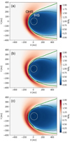 |
Fig. 7. Distributions of the plasma density in the B − V plane for the simulation time corresponding to: (a) 0, (b) 12.36, and (c) 37.75 years for a simulation that includes solar cycle effects. The inner white contour shows the position of the TS, the black points mark the position of the HP1 condition, and the green line marks the position of the HP2 condition. The Sun’s position is (0,0). |
In terms of the evolution of the HP, we can identify some changes in the location of the HP1 and HP2 conditions, which can be generally described as ripples. In general, there is a good match between the two HP definitions at the heliospheric nose for all the three snapshots shown in Fig. 7. As we move towards the heliospheric flanks, the two definitions diverge in the simulation space and also in their time evolution. For the maximum-slope-based HP1 condition, even an apparent discontinuity appears (see Fig. 7c, upper part) that results from the appearance of two local maxima in the derivative of the radial plasma density profile. The black points in Fig. 7, marking the HP1 location, were obtained for a number of directions from the Sun. It may happen that for a radial-plasma-density profile with two local maxima, one local maximum becomes larger than the second one as a result of a slight change in the direction. This gives the apparent discontinuities similar to what can be seen in Fig. 7c. However, we should note that this discontinuity results from the specific computation technique, that is, using the radial profiles in a region where the density-gradient direction is approximately perpendicular to the radial direction.
The relative variations of the TS, HP1, and HP2 conditions are better seen in Fig. 8, where the TS and HP positions are compared for the initial condition and the simulation time corresponding to 30.22 years. Apart from the small amplitude ripples, we can see anti-correlated shifts of the TS and upwind-hemisphere part of the HP, where the HP1 and HP2 conditions give similar locations. The shifts of the TS and HP have similarly small amplitudes at the heliospheric nose. If we consider the flanks of the heliosphere, the HP1 and HP2 conditions are different in terms of their locations and the amplitude of their time variations, the HP1 condition being more variable than HP2.
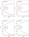 |
Fig. 8. Comparison of the TS, HP1 (upper panels, red color), and HP2 (lower panels, green color) positions for the initial condition (dashed line) and the solar-cycle simulation time corresponding to 30.22 years (solid line). Both B − V plane cut (HP1/XY and HP2/XY, the left column) and a perpendicular plane cut (HP1/XZ and HP2/XZ, the right column) through a three-dimensional solution are shown. |
We focus here on effects of the solar cycle on the density distribution and positions of the TS and HP, but it is worth mentioning that other variables, namely, the plasma velocity and temperature evolve significantly inside the heliosphere in accordance with the variation in the inner boundary condition. The influence of the solar cycle on the perpendicularity condition  is discussed further in a section devoted to a comparison of solar-cycle and LISM-fluctuation effects.
3.3. LISM perturbation – method description
In this simulation, a density perturbation is superposed on the stationary solution for B∞ = 0.3 nT and such modified solution is used as the initial condition for a time-dependent run. The density fluctuation is a pancake-like structure of a thickness of Lx = 100 AU (along LISM-flow axis) located initially in front of the heliosphere, as illustrated in Fig. 9. In two other directions, the structure is spatially extended, i.e., Ly = Lz ≫ 100 AU but it does not reach the boundary of the simulation domain, so constant-in-time boundary conditions can be still used. We note that our setting of the quasi-one-dimensional perturbation is similar to the plane-wave character of perturbations considered by Pogorelov (2000). However, Pogorelov (2000) considered periodic LISM fluctuations, while in our case, a solitary perturbation is analyzed to better separate effects of the passage of the structure through different regions (i.e., the nose vs. flanks of the heliosphere). Since only the plasma density is perturbed, the fluctuation corresponds to the entropy wave mode, which in the absence of the heliosphere and plasma-neutrals charge-exchange processes would be expected to be advected passively by the flow. However, in our simulation, the advection of the density enhancement by the LISM flow leads to the collision and interaction of the structure with the heliosphere. We should also note that the charge-exchange process in our simulation affects the evolution of the LISM structure, leading to a gradual change and a smoothing of the sharp gradients that have been set in the initial condition.
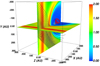 |
Fig. 9. Visualization of the initial condition in a time-dependent simulation of the interaction of a LISM fluctuation with the heliosphere. The plasma density np/np∞ distribution is shown in color. The LISM inflow is along x-axis. Black lines show some magnetic field lines starting in the B − V plane. Some of the magnetic field lines are draped onto the HP. Red planar structure in front of the simulated heliosphere is the LISM density perturbation. Close to the Sun located at (0,0,0), an internal heliospheric magnetic field line is shown (red line) in the form of a conical spiral. |
The amplitude of the density perturbation in the time-dependent simulation with a LISM fluctuation is set to δnp/np∞ = 1, which amounts to δnp = np∞ = 0.095 cm−3. The main rationale for this particular choice of the fluctuation amplitude is related to our attempts of comparing the effects of the solar cycle and the LISM fluctuation on the heliosphere. Since the LISM fluctuation involves only its hydrodynamic part, setting the dynamic-pressure increase to similar values in the solar cycle and LISM perturbation seems to provide a proper basis for comparison of the two effects. Our setting for the LISM perturbation corresponds to the dynamic pressure increase by the factor of ∼2. However, we must account for the suppression of the plasma density perturbations by the charge-exchange process that leads to a gradual decrease of the LISM-fluctuation amplitude before the interaction with the heliosphere. If we take the suppression into account, the dynamic-pressure increase for the solar cycle and the LISM perturbation are very similar in our setting.
A broader context for our choice of the LISM fluctuation amplitude can be discussed based on the interstellar turbulence spectrum P3N = 10−3k−11/3 of the electron density fluctuations (Armstrong et al. 1995). The spectrum was recently shown to agree for small scales up to ∼15 AU with the electron density fluctuations inferred from in-situ Voyager-1 measurements of the electrostatic plasma oscillations (Lee & Lee 2019). Using the spectrum for  (k is expressed in m−1) gives log10P3N ≈ 45.3 (for P3N given in m−3). Since
  , we get the average amplitude of density fluctuations
  cm−3, as inferred from the spectrum, which is two orders of magnitude smaller than our setting of δnp. However, we should bear in mind that “the Great Power Law in the Sky” of Armstrong et al. (1995) represents the results of various measurements composed together and fitted by an averaged spectrum extending over ∼45 orders of magnitude for the spectral density. Both in Fig. 1 in Armstrong et al. (1995) and in Fig. 2 in Lee & Lee (2019), particular measurements often deviate from the averaged spectrum by more than two orders of magnitude, but they still can be perceived to be consistent with the averaged spectrum due to the huge extent of the scales involved.
The measurements included in Fig. 1 from Armstrong et al. (1995), which are possibly closest to our scale of interest log10k ≈ −13.17, are denoted in the plot as “DM fluctuations” and they correspond to dispersion-measure observations for the interstellar scattering of pulsars radiation. If we interpolate the direct measurements for the group “DM fluctuations”, then for log10k ≈ −13.17 we get log10P3N ≈ 49.4, which corresponds to  cm−3, which is comparable to our setting δnp = 0.095 cm−3. This group of measurements is slightly above the averaged spectrum, but it represents more direct observational data than the averaged spectrum. Therefore, our amplitude setting can be considered to be consistent with particular measurement data, from which the averaged spectrum was composed.
3.4. LISM perturbation – results
Figure 10 shows distributions of the plasma density in the B − V plane. In an early stage of evolution (see Fig. 10a), the LISM fluctuation remains well separated from the density enhancement in the OHS. Further in time, the LISM fluctuation is advected by the LISM flow that eventually leads to a strong interaction on the part of the perturbation with the heliosphere as illustrated in Fig. 10b. At this stage, the HP is strongly compressed towards the Sun in the upwind hemisphere, while the HP1 and HP2 conditions are affected in a similar way. The LISM fluctuation undergoes a significant deformation related to the presence of the flow stagnation region in the OHS in front of the heliosphere. In the stagnation region, the advective transport of the LISM fluctuation slows down, while far from this region, the advection speed remains higher. In result, the deformation of the LISM fluctuation consists in wrapping up the structure onto the heliosphere. At a late stage of the evolution illustrated in Fig. 10c, we observe a recovery phase for the upwind hemisphere, where the distribution of the plasma density in the OHS gradually returns to its normal stationary case state. However, the effects of the interaction with the LISM fluctuation are now strongly affecting the downwind hemisphere, where flanks of the heliosphere are significantly squeezed.
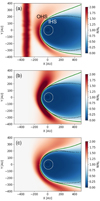 |
Fig. 10. Distributions of the plasma density in the B − V plane for the simulation time corresponding to: (a) 6.74, (b) 69.66, and (c) 119.1 years for simulations with the LISM fluctuation. The inner white contour shows the position of the TS, the black points mark the position of the HP1 condition, and the green line marks the position of the HP2 condition. The Sun position is (0,0). |
The effects of the LISM fluctuation on the positions of the TS and HP are illustrated in a more detail in Figs. 11 and 12. In the first stage of the interaction, for the simulation timeframe smaller than 65.17 years, the main effect is the compression of the heliosphere in the upwind hemisphere towards the Sun as shown in Fig. 11. Only a slight shift of the TS towards the Sun is seen at this stage. In the course of the system’s evolution, the upwind-hemisphere part of the heliosphere gradually returns to its normal state, while the effects of the interaction regularly shift to the downwind-hemisphere, leading to strong squeezing the flanks of the heliosphere (see Fig. 12). At this stage, the TS does not exhibit any significant shift with respect to the stationary solution. In the recovery phase, the HP1 condition seems to be less affected by the interaction of the heliosphere with the LISM perturbation, as compared with the HP2 condition.
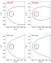 |
Fig. 11. Comparison of the TS, HP1 (upper panels, red color) and HP2 (lower panels, green color) positions for the initial condition (dashed line) and the LISM-fluctuation simulation time corresponding to 65.17 years (solid line). Both the B − V plane cut (HP1/XY and HP2/XY, the left column) and a perpendicular plane cut (HP1/XZ and HP2/XZ, the right column) through the three-dimensional solution are shown. |
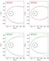 |
Fig. 12. Similar comparison as in Fig. 11, but at a later stage of the simulation with the LISM fluctuation. Positions of the TS, HP1 (upper panels, red color) and HP2 (lower panels, green color) are shown for the initial condition (dashed line) and the LISM-fluctuation simulation time corresponding to 139.3 years (solid line). |
Interestingly enough, we do not observe in our simulations any process of the sort of development of instabilities described in Pogorelov (2000). It could be that the magnetic field stabilizes the flow and suppresses the instabilities, as compared to the purely hydrodynamic case discussed by Pogorelov (2000). It is also possible that it is a matter of numerical diffusion due to the grid resolution (approximately several AU at the HP depending on the exact location of the HP relative to our spherically symmetric simulation grid). The grid is rather coarse due to relatively long simulated timescales in our time-dependent simulations of the interaction of the heliosphere with the LISM fluctuation.
3.5. Solar-cycle effects versus LISM perturbation – comparison
In Fig. 13, we present a comparison of the influence of the solar-cycle effects and the LISM fluctuation on the position of the TS and HP along the Voyager 1 and 2 trajectories. To test the generality of our results, two definitions of HP are used: HP1 – based on the maximum slope of the radial density profile and HP2 – based on loci of np(r) = np∞ in the radial profile (see Sect. 2.2). The position of the simulated TS is ∼60 AU, which makes the thickness of the IHS much larger than observed by Voyager 1 and 2. The measured position of the TS is also not reproduced in the work by Zirnstein et al. (2016), which we used to derive the boundary conditions for our study. As discussed in the literature, the problem of reproducing the measured thickness of the IHS presumably requires a sophisticated model of solar-cycle effects (Pogorelov et al. 2013) and specific thermodynamics of the IHS plasma (Izmodenov et al. 2014), which is not included in our modeling.
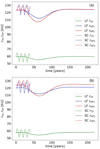 |
Fig. 13. Time dependence of the distance from the Sun to the TS and HP under the influence of the solar-cycle (SC – dashed line) and the LISM-fluctuation (LF – solid line) effects. Panel a: results for Voyager 1 and panel b – for Voyager 2. Green color shows results for the TS, and red/blue color – for the HP. Two HP definitions are used to test the generality of the simulation results. |
The most striking difference is related to different timescales associated with the solar-cycle effects (11 years) and the LISM fluctuation (80−90 years). The latter is consistent with a simple estimation of advection effects, which suggests a typical time scale of Δt = L0/v∞ ∼ 90 years, where L0 = 500 AU is taken as a typical global heliospheric spatial scale. Figure 13 suggests that for solar-cycle effects the amplitudes of the TS and HP motions are roughly similar (see dashed lines). For the HP2 definition, the HP motion amplitude in the solar cycle is slightly smaller than for the HP1 condition and even slightly smaller than the TS motion. A similar behavior (i.e., a smaller amplitude of the HP motion as compared to the TS) was reported, for example, by Zank & Müller (2003). On the contrary, in the case of the LISM fluctuation the response of the HP is much stronger than for the TS (solid lines). However, if the thickness of the IHS is considered, the simulations predict the following amplitudes for the solar-cycle simulation ∼22 AU (HP1 condition) and ∼17 AU (HP2 condition). For the LISM-perturbation simulation, it is ∼6 AU and ∼11 AU, respectively. Therefore, the solar-cycle-related thickness variations are generally larger than for the LISM perturbation, as inferred from Fig. 14. This is caused by a time delay between Sun-inward and Sun-outward phases of the motion of the TS and HP in the solar cycle. The time delay leads to anti-correlation of the motions of the TS and HP, which increases the amplitude of variations of the IHS thickness.
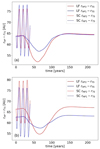 |
Fig. 14. Time dependence of the thickness of the IHS under the influence of the solar-cycle (SC – dashed line) and the LISM-fluctuation (LF – solid line) effects. Panel a: results for Voyager 1 and panel b – for Voyager 2. The two HP definitions are used to test the generality of the simulation results. |
Figure 15 shows that the LISM fluctuation affects the position of the simulated IBEX ribbon to a larger extent, as compared with the solar cycle effects. The average angular distance |Δθ| between the simulated perpendicularity condition and the observed IBEX ribbon shows unipolar variations for the solar cycle. By referring to unipolar variations, we mean that the variations cause only increase of the angular distance with respect to the stationary solution. In contrast, for the LISM fluctuation, the variation is bipolar, because for a time interval between ∼20 and ∼45 years, the angular distance is even smaller than for the stationary solution. The difference between the timescales associated with the solar-cycle and LISM-fluctuation effects is also visible for the simulated IBEX ribbon. In general, if we consider the magnitude of the deviation from the observed ribbon, the effects of the time-dependent effects are rather weak, that is, both the solar cycle and the LISM fluctuation do not cause large shifts of the  condition in the sky. For the solar cycle, the average angular distance oscillates between 1.8 < |Δθ|< 2.6 deg, while for the LISM fluctuation, the variation is 1.5 < |Δθ|< 3.0 deg. This suggests that the simulated ribbon position in the sky is stable, which is consistent with recent analysis of observational data by Dayeh et al. (2019). We should note that in Fig. 15, the HP2 definition was used, since the HP1 definition generates discontinuities in the HP location for the solar-cycle simulations (see Figs. 7 and 8 and related discussion), which makes it inappropriate for the analysis presented in Fig. 15.
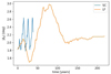 |
Fig. 15. Time dependence of the average angular distance |Δθ| between the simulated perpendicularity condition and the observed IBEX ribbon. The results are shown for the solar-cycle (SC – blue line) and the LISM-fluctuation (LF – orange line) effects. The average angular distance |Δθ| is computed using the locations of the simulated condition |

Figure 16 shows how the time-dependent shifts of the  condition (computed at 50 AU from the HP2 condition) appear in the sky. For the solar cycle, the first maximum deviation occurs for the simulation time of approximately 15.2 years. The corresponding map is shown in Fig. 16b. We can see that for the simulated ribbon (blue circles), the azimuthal-angle sector 315−100 deg moved slightly outward relative to the initial condition presented in Fig. 16a. For the LISM fluctuation, the variation is bipolar as discussed above, thus it is interesting to take a look both at the minimum and maximum value. The minimum value of |Δθ| occurs for the simulation time of 29.2 years. As shown in Fig. 16c, at this time, the simulated
  condition matches the observed ribbon even better, mainly due to an inward shift for the azimuthal-angle sector of 315−45 deg. This sector is physically located in the upwind hemisphere of the OHS. This part of the perpendicularity condition (blue circles) moves toward the ribbon center and thus closer to the observed ribbon (black circles). The maximum value of |Δθ| occurs for the simulation time of 78.7 years for the LISM fluctuation. As shown in Fig. 16d, parts of the ribbon responsible for the deviation are located in the azimuthal-angle sectors 195−280 and 110−125 deg. The sectors are physically located in the downwind hemisphere of the OHS (close to the flanks of the heliosphere). As we can see, the sector 195−280 deg moves toward the ribbon center and 110−125 deg sector moves outward as compared with the initial condition presented in Fig. 16a.
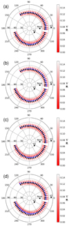 |
Fig. 16. Distributions of the simulated perpendicularity condition in the IBEX-ribbon-center frame for characteristic phases of time-dependent simulations. Black circles show the position of the observed IBEX ribbon, shades of red – color coded values of the simulated distribution of |


4. Discussion and conclusions
In the first part of our study, we investigated stationary solutions obtained with our model under the constant-hydrogen-flux approximation as compared with the fully kinetic modeling of neutrals by Zirnstein et al. (2016). In terms of the distance to the HP along the Voyager 1 trajectory, a relative difference between the two models amounts to up to ∼4.7% for the LISM magnetic field strength values between 0.2 and 0.4 nT. Similarly to the kinetic model, for the simulated IBEX ribbon, the best fit to observations is obtained for the LISM magnetic field strength of ∼0.3 nT. Distances to the HP obtained by our model are in reasonable agreement with Voyager 1 and 2 measurements. This analysis makes it possible to define a set of boundary conditions that provides the best fit of stationary solutions to observations, and which is then used as the initial condition in time-dependent simulations.
With regards to the comparison of the constant-hydrogen-flux model with kinetic simulations, the results presented in our paper are surprising if different models of the heliosphere are considered in terms of their increasing complexity. If the model complexity is taken into account, it is natural to expect that a multifluid model for neutrals should provide a better approximation as compared with the constant-flux approximation. However, a deeper insight into real physics is obtained if we consider spatial gradients of the moments of the distribution function for neutrals and effects introduced by a relatively large mean free path for neutrals in the heliosphere. As shown, for instance, by Alouani-Bibi et al. (2011), in their Fig. 9 (upper row of panels), multifluid models generate much steeper gradients (and, consequently, larger variations) of neutrals-distribution-function moments, as compared with kinetic modeling. These steep gradients are moderated in kinetic models due to effects introduced by a relatively large mean free path for neutral atoms in the heliosphere. These effects lead to smearing out the density, velocity, and temperature spatial distributions for neutrals. The constant-flux approximation that we use in our paper can be considered as an infinite-mean-free-path approximation, which is consistent with the assumption that the density, velocity, and temperature distributions for neutrals are completely flat throughout the heliosphere. On the other hand, fluid models for neutrals are, in fact, based on an implicit assumption of the zero mean free path. From this perspective, kinetic modeling turns out to be located somewhere between two limits represented by the multifluid and constant-flux approximations. Our paper provides an answer to how the constant-flux (or infinite-mean-free-path) approximation works in practice via a comparison of the heliopause location with kinetic-model results. Although more definitive conclusions would require a direct comparison of models for exactly the same boundary conditions, our results suggest that in some aspects, the constant-flux approximation may be superior to multifluid modeling of neutrals. In terms of the distance to the heliopause, according to Alexashov & Izmodenov (2005), multifluid models display discrepancies of 7−10% relative to the kinetic modeling, which is approximately two fold more than the ∼4.7% maximum discrepancy presented in our paper.
In the second part of the paper, we compare time-dependent effects introduced by the solar cycle and LISM fluctuations in the form of entropy waves. The most striking difference between the two types of drivers of time-dependent heliospheric phenomena is the time scale of the heliospheric response, which is approximately eight times longer for the LISM fluctuation. The amplitude of the HP motion along the Voyager spacecraft trajectories is ∼14 AU that translates to a relative deformation of ∼11%, which is much larger than the relative difference between the constant-hydrogen-flux and kinetic models (∼4.7% as discussed above). This result raises a question regarding limitations in fitting the LISM parameters based on matching stationary solutions to the measured distance to the HP. The question is quite important, since the vast majority of simulation studies focused on inferring the LISM parameters have been based on stationary solutions. Since we cannot exclude a priori that the heliosphere is moving on a gradient of the LISM plasma density, such stationary-solution-based estimations can have limited accuracy. In this context, the IBEX ribbon seems to be a relatively stable structure that does not change its center in the sky substantially under the influence of time-dependent phenomena investigated in our paper. However, slight systematic changes in the position of the IBEX ribbon in its different sectors (i.e., changes in the heliospheric nose followed by variations in the heliospheric flanks) may serve as an indicator of a passage of a density fluctuation in the LISM, as suggested by our study.
Our results show that in terms of reducing the thickness of the heliosheath, the solar cycle has stronger effect than the LISM fluctuation with regard to the magnitude of the reduction. However, we ought to bear in mind that associated mechanisms of the reduction are different. For solar cycle effects, we observe anti-correlation between the motion of the TS and HP due to a time delay between the propagation of the solar cycle effects to the two discontinuities. In contrast, in the case of the LISM fluctuation, the amplitude of the HP motion is much larger than for the TS. Generally, the time-dependent effects investigated in our paper lead to relative changes in the IHS thickness on the order of approximately 10−30%.
Our study sheds new light on the question of possible detection of variations of parameters of the interstellar environment of the Sun, for example, by observing the evolution of the IBEX ribbon on long timescales. In this context, an extension of the observations of the IBEX mission by the IMAP satellite plays a crucial role (McComas et al. 2018).
Acknowledgments
Calculations were carried out at the Centre of Informatics, Tricity Academic Supercomputer & Network.
References
- Alexashov, D., & Izmodenov, V. 2005, A&A, 439, 1171 [NASA ADS] [CrossRef] [EDP Sciences] [Google Scholar]
- Alouani-Bibi, F., Opher, M., Alexashov, D., Izmodenov, V., & Toth, G. 2011, ApJ, 734, 45 [NASA ADS] [CrossRef] [Google Scholar]
- Armstrong, J. W., Rickett, B. J., & Spangler, S. R. 1995, ApJ, 443, 209 [Google Scholar]
- Borovikov, S. N., Pogorelov, N. V., Zank, G. P., & Kryukov, I. A. 2008, ApJ, 682, 1404 [NASA ADS] [CrossRef] [Google Scholar]
- Burlaga, L. F., Ness, N. F., & Stone, E. C. 2013, Science, 341, 147 [NASA ADS] [CrossRef] [Google Scholar]
- Burlaga, L. F., Ness, N. F., Berdichevsky, D. B., et al. 2019, Nat. Astron., 3, 1007 [NASA ADS] [CrossRef] [Google Scholar]
- Chalov, S. V., Alexashov, D. B., McComas, D., et al. 2010, ApJ, 716, L99 [NASA ADS] [CrossRef] [Google Scholar]
- Dayeh, M. A., Zirnstein, E. J., Desai, M. I., et al. 2019, ApJ, 879, 84 [NASA ADS] [CrossRef] [Google Scholar]
- Florinski, V. 2015, ApJ, 813, 49 [NASA ADS] [CrossRef] [Google Scholar]
- Florinski, V., Zank, G. P., Heerikhuisen, J., Hu, Q., & Khazanov, I. 2010, ApJ, 719, 1097 [NASA ADS] [CrossRef] [Google Scholar]
- Frisch, P., & Dwarkadas, V. V. 2018, ArXiv e-prints [arXiv:1801.06223] [Google Scholar]
- Funsten, H. O., Allegrini, F., Crew, G. B., et al. 2009, Science, 326, 964 [NASA ADS] [CrossRef] [Google Scholar]
- Funsten, H. O., DeMajistre, R., Frisch, P. C., et al. 2013, ApJ, 776, 30 [CrossRef] [Google Scholar]
- Gurnett, D. A., & Kurth, W. S. 2019, Nat. Astron., 3, 1024 [NASA ADS] [CrossRef] [Google Scholar]
- Heerikhuisen, J., Pogorelov, N. V., Zank, G. P., et al. 2010, ApJ, 708, L126 [NASA ADS] [CrossRef] [Google Scholar]
- Izmodenov, V. V., Malama, Y. G., & Ruderman, M. S. 2008, Adv. Space Res., 41, 318 [NASA ADS] [CrossRef] [Google Scholar]
- Izmodenov, V. V., Alexashov, D. B., & Ruderman, M. S. 2014, ApJ, 795, L7 [NASA ADS] [CrossRef] [Google Scholar]
- Kim, T. K., Pogorelov, N. V., Zank, G. P., Elliott, H. A., & McComas, D. J. 2016, ApJ, 832, 72 [NASA ADS] [CrossRef] [Google Scholar]
- Krimigis, S. M., Decker, R. B., Roelof, E. C., et al. 2013, Science, 341, 144 [NASA ADS] [CrossRef] [Google Scholar]
- Lallement, R., Quémerais, E., Koutroumpa, D., et al. 2010, in Twelfth International Solar Wind Conference, eds. M. Maksimovic, K. Issautier, N. Meyer-Vernet, M. Moncuquet, & F. Pantellini, AIP Conf. Ser., 1216, 555 [NASA ADS] [Google Scholar]
- Lee, K. H., & Lee, L. C. 2019, Nat. Astron., 3, 154 [Google Scholar]
- McComas, D. J., Allegrini, F., Bochsler, P., et al. 2009, Science, 326, 959 [NASA ADS] [CrossRef] [Google Scholar]
- McComas, D. J., Christian, E. R., Schwadron, N. A., et al. 2018, Space Sci. Rev., 214, 116 [CrossRef] [Google Scholar]
- Michael, A. T., Opher, M., Provornikova, E., Richardson, J. D., & Tóth, G. 2015, ApJ, 803, L6 [NASA ADS] [CrossRef] [Google Scholar]
- Müller, H. R., Frisch, P. C., Fields, B. D., & Zank, G. P. 2009, Space Sci. Rev., 143, 415 [CrossRef] [Google Scholar]
- Pogorelov, N. V. 2000, Astrophys. Space Sci., 274, 115 [NASA ADS] [CrossRef] [Google Scholar]
- Pogorelov, N. V., Suess, S. T., Borovikov, S. N., et al. 2013, ApJ, 772, 2 [NASA ADS] [CrossRef] [Google Scholar]
- Pogorelov, N. V., Heerikhuisen, J., Roytershteyn, V., et al. 2017, ApJ, 845, 9 [NASA ADS] [CrossRef] [Google Scholar]
- Ratkiewicz, R., Ben-Jaffel, L., & Grygorczuk, J. 2008, in Numerical Modeling of Space Plasma Flows, eds. N. V. Pogorelov, E. Audit, & G. P. Zank, ASP Conf. Ser., 385, 189 [NASA ADS] [Google Scholar]
- Ratkiewicz, R., Strumik, M., & Grygorczuk, J. 2012, ApJ, 756, 3 [NASA ADS] [CrossRef] [Google Scholar]
- Richardson, J. D., Belcher, J. W., Garcia-Galindo, P., & Burlaga, L. F. 2019, Nat. Astron., 3, 1019 [NASA ADS] [CrossRef] [Google Scholar]
- Scherer, K., & Fahr, H. J. 2003, Geophys. Res. Lett., 30, 1045 [NASA ADS] [CrossRef] [Google Scholar]
- Schwadron, N. A., & McComas, D. J. 2013, ApJ, 764, 92 [NASA ADS] [CrossRef] [Google Scholar]
- Schwadron, N. A., Bzowski, M., Crew, G. B., et al. 2009, Science, 326, 966 [NASA ADS] [CrossRef] [Google Scholar]
- Stone, E. C., Cummings, A. C., McDonald, F. B., et al. 2013, Science, 341, 150 [NASA ADS] [CrossRef] [Google Scholar]
- Strumik, M., Ben-Jaffel, L., Ratkiewicz, R., & Grygorczuk, J. 2011, ApJ, 741, L6 [NASA ADS] [CrossRef] [Google Scholar]
- Strumik, M., Czechowski, A., Grzedzielski, S., Macek, W. M., & Ratkiewicz, R. 2013, ApJ, 773, L23 [CrossRef] [Google Scholar]
- Strumik, M., Grzedzielski, S., Czechowski, A., Macek, W. M., & Ratkiewicz, R. 2014, ApJ, 782, L7 [CrossRef] [Google Scholar]
- Swisdak, M., Drake, J. F., & Opher, M. 2013, ApJ, 774, L8 [NASA ADS] [CrossRef] [Google Scholar]
- Washimi, H., Zank, G. P., Hu, Q., et al. 2011, MNRAS, 416, 1475 [CrossRef] [Google Scholar]
- Zank, G. P., & Müller, H. R. 2003, J. Geophys. Res., 108, 1240 [NASA ADS] [CrossRef] [Google Scholar]
- Zirnstein, E. J., Heerikhuisen, J., Funsten, H. O., et al. 2016, ApJ, 818, L18 [CrossRef] [Google Scholar]
- Zirnstein, E. J., McComas, D. J., Schwadron, N. A., et al. 2019, ApJ, 876, 92 [NASA ADS] [CrossRef] [Google Scholar]
All Tables
All Figures
|
Fig. 1. Simulated density profile along Voyager 1 and 2 trajectories for the case where B∞ = 0.3 nT. Locations of three HP definitions are shown in the plot: HP1 (based on the maximum slope of the density profile), HP2 (isocontour np = np∞) and separatrix-based definition HP SEP. The inset shows in detail the region embraced by dashed lines in the main plot. The main plot uses the logarithmic vertical scale, while in the inset, the vertical scale is linear. |
| In the text | |
|
Fig. 2. Shape of the HP according to three different definitions for a stationary solution for the LISM magnetic field strength B∞ = 0.3 nT. Definitions HP1 and HP2 are based on the density profile and the definition HP SEP is the separatrix between the heliospheric and LISM flows computed from streamline analysis. Both the B − V-plane cut (on the left) and the perpendicular-plane cut (on the right) through the three-dimensional solution are shown. |
| In the text | |
|
Fig. 3. Distance to the HP along the Voyager 1 (red) and 2 (blue) trajectories for different boundary conditions of the simulation parametrized by the strength of the unperturbed LISM magnetic field. The solid lines show the heliopause location according to the HP1 definition, while dashed lines show the location of the separatrix resulting from streamline analysis. |
| In the text | |
|
Fig. 4. Distributions of the simulated perpendicularity condition in the IBEX-ribbon-center frame. Black circles show the position of the observed IBEX ribbon, shades of red color-coded values of the simulated distribution of |
| In the text | |
|
Fig. 5. Dependence on the distance from the HP (HP1 definition) of the average angular distance |Δθ| between the simulated perpendicularity condition and the observed IBEX ribbon for different LISM magnetic field strengths, shown in panel a. Panel b: how the minimum of each profile in panel a depends on the LISM magnetic field strength. Colors of circles in panel b correspond to colors of lines in panel a. The minimum of the simulated dependence shown in panel b gives an estimate of the LISM magnetic field strength that provides the best fit to IBEX ribbon observations. |
| In the text | |
|
Fig. 6. Similar dependence as presented in Fig. 5 but for the HP2 definition of the heliopause. The dependence of |Δθ| on the distance from the HP (HP2 definition) is shown in panel a. Panel b: how the minimum of each profile in panel a depends on the LISM magnetic field strength. |
| In the text | |
|
Fig. 7. Distributions of the plasma density in the B − V plane for the simulation time corresponding to: (a) 0, (b) 12.36, and (c) 37.75 years for a simulation that includes solar cycle effects. The inner white contour shows the position of the TS, the black points mark the position of the HP1 condition, and the green line marks the position of the HP2 condition. The Sun’s position is (0,0). |
| In the text | |
|
Fig. 8. Comparison of the TS, HP1 (upper panels, red color), and HP2 (lower panels, green color) positions for the initial condition (dashed line) and the solar-cycle simulation time corresponding to 30.22 years (solid line). Both B − V plane cut (HP1/XY and HP2/XY, the left column) and a perpendicular plane cut (HP1/XZ and HP2/XZ, the right column) through a three-dimensional solution are shown. |
| In the text | |
|
Fig. 9. Visualization of the initial condition in a time-dependent simulation of the interaction of a LISM fluctuation with the heliosphere. The plasma density np/np∞ distribution is shown in color. The LISM inflow is along x-axis. Black lines show some magnetic field lines starting in the B − V plane. Some of the magnetic field lines are draped onto the HP. Red planar structure in front of the simulated heliosphere is the LISM density perturbation. Close to the Sun located at (0,0,0), an internal heliospheric magnetic field line is shown (red line) in the form of a conical spiral. |
| In the text | |
|
Fig. 10. Distributions of the plasma density in the B − V plane for the simulation time corresponding to: (a) 6.74, (b) 69.66, and (c) 119.1 years for simulations with the LISM fluctuation. The inner white contour shows the position of the TS, the black points mark the position of the HP1 condition, and the green line marks the position of the HP2 condition. The Sun position is (0,0). |
| In the text | |
|
Fig. 11. Comparison of the TS, HP1 (upper panels, red color) and HP2 (lower panels, green color) positions for the initial condition (dashed line) and the LISM-fluctuation simulation time corresponding to 65.17 years (solid line). Both the B − V plane cut (HP1/XY and HP2/XY, the left column) and a perpendicular plane cut (HP1/XZ and HP2/XZ, the right column) through the three-dimensional solution are shown. |
| In the text | |
|
Fig. 12. Similar comparison as in Fig. 11, but at a later stage of the simulation with the LISM fluctuation. Positions of the TS, HP1 (upper panels, red color) and HP2 (lower panels, green color) are shown for the initial condition (dashed line) and the LISM-fluctuation simulation time corresponding to 139.3 years (solid line). |
| In the text | |
|
Fig. 13. Time dependence of the distance from the Sun to the TS and HP under the influence of the solar-cycle (SC – dashed line) and the LISM-fluctuation (LF – solid line) effects. Panel a: results for Voyager 1 and panel b – for Voyager 2. Green color shows results for the TS, and red/blue color – for the HP. Two HP definitions are used to test the generality of the simulation results. |
| In the text | |
|
Fig. 14. Time dependence of the thickness of the IHS under the influence of the solar-cycle (SC – dashed line) and the LISM-fluctuation (LF – solid line) effects. Panel a: results for Voyager 1 and panel b – for Voyager 2. The two HP definitions are used to test the generality of the simulation results. |
| In the text | |
|
Fig. 15. Time dependence of the average angular distance |Δθ| between the simulated perpendicularity condition and the observed IBEX ribbon. The results are shown for the solar-cycle (SC – blue line) and the LISM-fluctuation (LF – orange line) effects. The average angular distance |Δθ| is computed using the locations of the simulated condition |
| In the text | |
|
Fig. 16. Distributions of the simulated perpendicularity condition in the IBEX-ribbon-center frame for characteristic phases of time-dependent simulations. Black circles show the position of the observed IBEX ribbon, shades of red – color coded values of the simulated distribution of |
| In the text | |
Current usage metrics show cumulative count of Article Views (full-text article views including HTML views, PDF and ePub downloads, according to the available data) and Abstracts Views on Vision4Press platform.
Data correspond to usage on the plateform after 2015. The current usage metrics is available 48-96 hours after online publication and is updated daily on week days.
Initial download of the metrics may take a while.