| Issue |
A&A
Volume 657, January 2022
|
|
|---|---|---|
| Article Number | A19 | |
| Number of page(s) | 20 | |
| Section | Extragalactic astronomy | |
| DOI | https://doi.org/10.1051/0004-6361/202140414 | |
| Published online | 21 December 2021 | |
Scaling relations and baryonic cycling in local star-forming galaxies
III. Outflows, effective yields, and metal loading factors
1
INAF – Osservatorio Astronomico di Capodimonte, Salita Moiariello 16, 80131 Napoli, Italy
e-mail: This email address is being protected from spambots. You need JavaScript enabled to view it.
2
INAF – Osservatorio Astrofisico di Arcetri, Largo Enrico Fermi 5, 50125 Firenze, Italy
3
European Southern Observatory, Karl-Schwarzschild-Straße 2, 85748 Garching, Germany
4
Observatoire de Genève, Université de Genève, 51 Ch. des Maillettes, 1290 Versoix, Switzerland
Received:
25
January
2021
Accepted:
4
October
2021
Abstract
Gas accretion and stellar feedback processes link metal content, star formation, and gas and stellar mass (and the potential depth) in star-forming galaxies. Constraining this hypersurface has been challenging because of the need for measurements of H I and H2 gas masses spanning a broad parameter space. A recent step forward has been achieved through the Metallicity And Gas for Mass Assembly sample of local star-forming galaxies, which consists of homogeneously determined parameters and a significant quantity of dwarf galaxies, with stellar masses as low as ∼105 − 106 M⊙. Here, in the third paper of a series, we adopt a standard galactic chemical evolution model, with which we can quantify stellar-driven outflows. In particular, we constrain the difference between the mass-loading in accretion and outflows and the wind metal-loading factor. The resulting model reproduces very well the local mass–metallicity relation, and the observed trends of metallicity with gas fraction. Although the difference in mass loading between accreted and expelled gas is extremely difficult to constrain, we find indications that, on average, the amount of gas acquired through accretion is roughly the same as the gas lost through bulk stellar outflows, a condition roughly corresponding to a “gas equilibrium” scenario. In agreement with previous work, the wind metal-loading factor shows a steep increase toward lower mass and circular velocity, indicating that low-mass galaxies are more efficient at expelling metals, thus shaping the mass–metallicity relation. Effective yields are found to increase with mass up to an inflection mass threshold, with a mild decline at larger masses and circular velocities. A comparison of our results for metal loading in outflows with the expectations for their mass loading favors momentum-driven winds at low masses, rather than energy-driven ones.
Key words: galaxies: star formation / galaxies: ISM / galaxies: fundamental parameters / galaxies: statistics / galaxies: dwarf / evolution
© ESO 2021
1. Introduction
Star-forming galaxies evolve and assemble their mass by accreting gas from the intergalactic medium (IGM), converting it in stars, then expelling gas and metals, thus changing the gas metallicity in the interstellar medium (ISM). This baryon cycle is mainly regulated by internal processes1 (e.g., Wu et al. 2017), which are responsible for metal and dust production, and the subsequent expulsion of material. Outflows driven by stellar winds and supernovae (SNe) explosions dominate in the lower-mass regime, while at higher masses, outflows tend to be powered by feedback from active galactic nuclei (AGN, e.g., Tremonti et al. 2004; Dekel & Birnboim 2006; Dalcanton 2007; Erb 2008; Finlator & Davé 2008; Zahid et al. 2014; De Rossi et al. 2017; Lara-López et al. 2019).
The efficiency of these processes is predicted to change with galaxy properties, and in particular with the virial mass (Mvir) and stellar mass (Mstar) of the galaxies. These variations lead to the most important relations among the main galaxy parameters driving galaxy evolution, namely the “main sequence” correlation between Mstar and the star-formation rate (SFR, e.g., Brinchmann et al. 2004, the SFMS); the mass–metallicity relation (e.g., Tremonti et al. 2004, the MZR); and the consequent inverse correlation between metallicity and specific SFR (sSFR ≡ SFR/Mstar, e.g., Mannucci et al. 2010; Lara-López et al. 2010; Hunt et al. 2012, 2016). Baryonic processes are thought to shape the SFMS and the MZR, in addition to many other correlations among other stellar properties and dark matter: the virial-to-stellar mass (e.g., Moster et al. 2010) and the baryonic Tully–Fisher (e.g., Lelli et al. 2016a) relations; the correlation between color and stellar population gradients with mass (e.g., Tortora et al. 2010); and the relation of dark matter fraction and mass density slopes with stellar mass (e.g., Tortora et al. 2019).
These scaling relations are not necessarily straight power laws, but can also show curvatures, bending, breaks, and U-shapes, suggesting the existence of typical mass scales which regulate the efficiency of the physical processes involved in baryonic cycling (e.g., Dekel & Birnboim 2006). Kannappan et al. (2013) identified two transitions in galaxy morphology, gas fractions, and fueling regimes. The first transition was considered a “gas-richness” threshold; galaxies below a transition mass of log(Mstar/M⊙) ∼ 9.5 were found to be “accretion-dominated”, characterized by overwhelming gas accretion. The second Mstar transition corresponds, instead, to a bimodality threshold, roughly indicating a “quenched” regime at log(Mstar/M⊙) > 10.5, populated by spheroid-dominated, gas-poor galaxies.
Both Mstar thresholds, and the mass regimes they delineate, are really tracing gas content, and its intimate link with star-formation activity (Kannappan et al. 2013). To further explore this link, in the first paper of this series (Ginolfi et al. 2020, hereafter Paper I), we constructed a sample of galaxies in the Local Universe with homogeneously derived global measurements of the main parameters that quantify galaxy evolution: namely Mstar, SFR, metallicity O/H, and gas content including molecular gas mass MH2 and atomic gas mass MHI. The sample comprises ∼400 galaxies, and was dubbed Metallicity And Gas for Mass Assembly (MAGMA).
In a second paper (Hunt et al. 2020, hereafter Paper II), we used MAGMA to explore how molecular and atomic gas properties vary as a function of Mstar and SFR. The main focus of Paper II was on feedback processes, and how they govern scaling relations across the mass spectrum. Essentially three processes play a role in regulating galaxy evolution2: (P1) preventive feedback, the (lack of) availability of cold baryons from the host halo; (P2) inefficiency of the star-formation process, the conversion of the available gas into stars; and (P3) ejective feedback, the production of energy and momentum, and the expulsion of material including gas, dust, and metals. In Paper II, we investigated two of the three main feedback mechanisms behind the inefficiency of low-mass halos to form stars (e.g., Behroozi et al. 2013; Moster et al. 2013; Graziani et al. 2015, 2017): namely the availability of cold gas to form stars (P1), and the inefficiency of the star-formation process itself (P2).
Here, in the third paper of the series, we examine the remaining mechanism, (P3), the efficiency of metal enrichment and ejective feedback. Understanding the processes that shape galaxy scaling relations with metallicity has proved to be a challenging task. It has been historically important to compare observations with the “closed-box” model, assuming that the total baryon content in the galaxy is fixed and the gas and stellar content are only determined by star formation and the stellar yields (e.g., Pagel & Patchett 1975). However, it is widely recognized that galaxies do not evolve as closed boxes (e.g., Tremonti et al. 2004), and more complex models have considered inflows and outflows of material from the galactic ecosystem (e.g., Larson 1972; Pagel & Patchett 1975; Tinsley 1980; Pagel & Edmunds 1981; Edmunds & Pagel 1984; Edmunds 1990; Tremonti et al. 2004; Dalcanton 2007; Erb 2008; Finlator & Davé 2008; Recchi et al. 2008; Peeples & Shankar 2011; Dayal et al. 2013; Zahid et al. 2014; Peng & Maiolino 2014). More recently, hydrodynamical simulations have tested these predictions (e.g., Ma et al. 2016; De Rossi et al. 2017; Torrey et al. 2019).
Our approach here is mainly empirical, requiring a sample with measurements of Mstar, SFR, O/H, and gas content, homogeneously determined over a wide range of stellar mass and gas fractions; MAGMA is such a sample. In this paper, Sect. 2 describes briefly the MAGMA sample and how it was assembled. Then, Sect. 3 presents the theoretical formalism for metallicity evolution and the scaling of metallicity with Mstar, SFR, and gas content. The computation of outflow parameters and metal-loading factors for MAGMA galaxies is described in Sect. 4, and their impact on shaping the mass–metallicity relation in Sect. 5. We recast our results in the context of the effective yields in Sect. 6, and discuss the physical implications for wind metallicity and mass loading of the winds in Sect. 7. Our conclusions are drawn in Sect. 8.
2. MAGMA sample
Paper I presented the MAGMA sample, comprising 392 local galaxies having homogeneously derived global quantities including Mstar, SFR, metallicities [12 + log(O/H)], and gas masses (both atomic, MHI, and molecular, MH2, and total Mg = MHI + MH2). Molecular gas masses were obtained by measurements of the CO luminosity,  . We assembled this sample by combining a variety of previous surveys at z ∼ 0 with new observations of CO in low-mass galaxies. Only galaxies with robust detections of physical parameters were retained, that is to say we required clear detections of CO and H I. Galaxies were eliminated if they showed optical signatures of an AGN in the parent samples (obtained from line-ratio diagnostics, similar to Baldwin et al. 1981). We also eliminated potentially H I-deficient galaxies by applying a cut based on H I-deficiency measurements, where available (e.g., Boselli et al. 2009, 2014a). The MAGMA sample spans more than 5 orders of magnitude in Mstar, SFR, and Mg, and a factor of ∼50 in metallicity [Z, 12 + log(O/H)].
Because of potential systematics that could perturb our results, in Paper I we homogenized the sample by recalculating both Mstar and SFR in a uniform way. To calculate SFR, we adopted the hybrid formulations of Leroy et al. (2019), based on combinations of GALEX and WISE luminosities. New Mstar measurements were computed using 3.4 μm (or IRAC 3.6 μm when not available) luminosities from fluxes in the ALLWISE Source Catalogue (Wright et al. 2010) and a luminosity-dependent M/L from Hunt et al. (2019); the continuum contribution from free-free emission was subtracted from these luminosities before the Mstar computation. Both SFR and Mstar assume a Chabrier (2003) IMF.
For metallicity, 12 + log(O/H), we adopted either “direct” calibrations, based on electron temperatures (e.g., Izotov et al. 2007), or the [N II]-based strong-line calibration by Pettini & Pagel (2004, PP04N2). When PP04N2-derived metallicities were not available, they were converted from the original calibration to PP04N2 according to Kewley & Ellison (2008). PP04N2 is the metallicity calibration closest to the direct one (e.g., Andrews & Martini 2013; Hunt et al. 2016), which makes it appropriate for a sample like MAGMA that spans a wide range of Mstar and SFR.
The molecular gas mass was determined from  based mainly on 12CO(1 − 0); only in a few cases did we have to convert from 12CO(2 − 1) to 12CO(1 − 0) using “standard” prescriptions (e.g., Leroy et al. 2009; Schruba et al. 2012). The conversion factor αCO from CO luminosity to molecular gas mass was calculated according to the piecewise relation presented in Paper II, with αCO ∝ Z1.55, for 12 + log(O/H) < 8.69 and
  (K km s−1 pc2)−1 (see also Saintonge et al. 2011). The impact of a different metallicity dependence is discussed in Paper II. Here we do not include a factor of 1.36 to account for helium. For more details about the parent surveys, as well as parameter determinations and calibrations, quality checks, or the derivation of scaling relations, we refer the reader to Paper I and Paper II.
3. Metallicity evolution and scaling relations: formalism
Much effort has been spent over the last fifty years to understand the theoretical framework behind the baryon exchange cycle and metallicity evolution in galaxies (e.g., Larson 1972; Pagel & Patchett 1975; Tinsley 1980; Pagel & Edmunds 1981; Edmunds & Pagel 1984; Edmunds 1990; Tremonti et al. 2004; Dalcanton 2007; Erb 2008; Finlator & Davé 2008; Recchi et al. 2008; Spitoni et al. 2010; Peeples & Shankar 2011; Dayal et al. 2013; Zahid et al. 2014; Peng & Maiolino 2014). It has been fairly well established that bulk outflows and galactic winds driven by star formation are necessary to explain the MZR and other scaling relations involving metallicity. Here we follow these pioneering works, and explore the behavior of the MZR, SFR, and gas content in the MAGMA galaxies. MAGMA provides the important constraints of gas measurements together with SFR and metallicity, thus enabling, for the first time, a quantification of the mass and metallicity loading in stellar outflows, and their role in shaping the MZR in the Local Universe.
3.1. Galactic chemical evolution
In what follows, we rely heavily on the formulations for galactic chemical evolution by Pagel (2009). We first make the assumption of instantaneous recycling, namely that the chemical enrichment provided by stellar evolution, nucleosynthesis, and expulsion of metals into the ISM take place “instantaneously” relative to the timescales of overall galaxy evolution.
There are two main quantities that this assumption makes time-invariant: the first is the return fraction R, the mass fraction of a single stellar generation that is returned to the ISM; the second is the (true) stellar yield, y, defined as the mass of an element newly produced and expelled by a generation of stars relative to the mass that remains locked up in long-lived stars and compact remnants. The metal mass produced relative to the initial mass of a single stellar generation is then q = α y where α = 1 − R, (or “lock-up” fraction), with the implicit assumption that stellar lifetimes can be neglected so that R is a net mass return fraction (see e.g., Vincenzo et al. 2016).
These parameters are governed by the IMF, and in particular the mass fraction of a stellar generation above a certain limit, since these are the main contributors to metal production. We further assume that metals are homogeneously mixed at all times, and that initally there are no stars and no metals, only the initial gas Mg(t = 0) with mass Mi.
There are four main physical quantities involved in and constrained by chemical evolution: the mass in stars, Mstar; the star-formation rate SFR, here referred to as ψ; the mass in gas, Mg; and the mass in metals, MZ, or the metal abundance in the gas, Zg = MZ/Mg. The mass of stars that have been born up to time t can be written as:
 (1)
(1)
Consequently, the mass Mstar remaining in stars and long-lived remnants is:
 (2)
(2)
The total baryonic mass in a galactic system is the sum of gas and stars:
 (3)
(3)
where Mw is the mass expelled in bulk winds and outflows, and Ma is the mass of newly accreted gas. This is essentially a mass continuity equation that defines the mass conservation between infall, outflows, and star formation. Thus, the time derivative of the gas mass can be written as:
 (4)
(4)
The time variation of the mass of metals MZ in the ISM gas depends on ψ, R, the stellar yield q, Ṁa, and Ṁw as follows:
 (5)
(5)
where Za and Zw are the metallicities of the accreted and outflow gas, respectively. The first two terms on the right-hand side of Eq. (5) correspond to the addition of metals of ejecta from stars; the third term to the loss to the ISM from astration; and the remaining terms to the metals gained from accretion and lost in bulk stellar outflows from winds and SNe.
Equation (5) can be simplified by two common assumptions: we take Ṁa and Ṁw to be directly proportional to ψ (e.g., Erb 2008; Peeples & Shankar 2011; Dayal et al. 2013; Lilly et al. 2013):
 (6)
(6)
where we have introduced the mass-loading factors ηa and ηw. It is fairly well established that the latter relation is true, namely that the mass in outflows is proportional to SFR, at least to its integral over time (e.g., Muratov et al. 2015; Christensen et al. 2016). In contrast, the former proportionality is more subject to speculation, although evidence is mounting that gas accretion powers star formation (e.g., Fraternali & Tomassetti 2012; Sánchez Almeida et al. 2014; Tacchella et al. 2016). In any case, this assumption provides the noteable advantage of analytical simplicity; we plan to investigate more completely its ramifications in a future paper. Following Peeples & Shankar (2011), we also introduce the metal-loading factors ζa and ζw relating Zg, Za, ηa, Zw, and ηw:
 (7)
(7)
and
 (8)
(8)
ζw and ζa essentially describe the efficiency with which gas accretion and star-formation-driven outflows change metal content within the galaxy. Thus, we can rewrite Eqs. (4) and (5) as:
 (9)
(9)
and
![Mathematical equation: $$ \begin{aligned} \dot{M}_Z = \psi \,[q - \alpha \,Z_{\rm g} + Z_{\rm g}\,(\zeta _{\rm a} - \zeta _{\rm w})]. \end{aligned} $$](/articles/aa/full_html/2022/01/aa40414-21/aa40414-21-eq13.gif) (10)
(10)
Our observations do not directly constrain MZ, but rather Zg, so we need to reformulate Eq. (10):
 (11)
(11)
in order to solve for Żg:
![Mathematical equation: $$ \begin{aligned} \dot{Z}_{\rm g} = \frac{\psi }{M_{\rm g}}\,[q + Z_{\rm g}\,(\zeta _{\rm a} - \zeta _{\rm w} - \eta _{\rm a} + \eta _{\rm w})], \end{aligned} $$](/articles/aa/full_html/2022/01/aa40414-21/aa40414-21-eq15.gif) (12)
(12)
where we have used Eq. (9) for Ṁg and Eq. (10) for ṀZ.
The necessary ingredients are now in place to derive the solution for the dependence of Zg on the remaining parameters. First, we know that SFR is related to gas mass by:
 (13)
(13)
where ϵ⋆ is the inverse depletion time or time-scale for star formation. Equations (9) and (13) are coupled, so must be solved simultaneously. Assuming that ϵ⋆ does not vary with time, we can thus integrate Eq. (9), to obtain the following solution for the gas mass:
 (14)
(14)
Substituting this solution into Eq. (12) and integrating, we obtain:
![Mathematical equation: $$ \begin{aligned} Z_{\rm g} = \left(\frac{q}{\zeta _{\rm w} - \zeta _{\rm a} + \eta _{\rm a} - \eta _{\rm w}}\right)\, \left[1 - \left(\frac{M_{\rm g}}{M_{\rm i}}\right)^{\frac{\zeta _{\rm a} - \zeta _{\rm w} - \eta _{\rm a} + \eta _{\rm w}}{\eta _{\rm a} - \eta _{\rm w} - \alpha }}\right], \end{aligned} $$](/articles/aa/full_html/2022/01/aa40414-21/aa40414-21-eq18.gif) (15)
(15)
where it can be seen that the time dependence is encapsulated in the evolution of the gas (Mg/Mi, e.g., Recchi et al. 2008). Equation (15) is essentially telling us that galaxies evolve along a hypersurface constrained by Mstar, Mg, gas metallicity, and accretion and wind mass and metal loadings. The galaxy’s position on this hypersurface can change with time as gas is accreted, stars are formed, and mass and metals are ejected in winds. However, at each time, the relation constraining these fundamental variables is approximately invariant.
The ratio of the system gas mass Mg and the initial gas mass Mi can be written in terms of the baryonic gas mass fraction, μg = Mg/(Mg + M⋆):
 (16)
(16)
where we have assumed that the total baryonic mass is described by Eq. (3). This is again an expression of mass conservation, meaning that no gas has been expelled altogether from the galaxy, but rather has been recycled into stars as described in Eq. (13).
Similar solutions for Zg were first formulated by Edmunds & Pagel (1984), and later by Recchi et al. (2008), Erb (2008), Spitoni et al. (2010), Peeples & Shankar (2011), Dayal et al. (2013), and many others. These earlier works mostly assumed that Zw/Zg = 1 in a so-called homogeneous wind (e.g., Pagel 2009), leading to ζw = ηw. This assumption simplifies Eq. (15) placing the dependence of ηw only in the exponent of Mg/Mi. However, as has been shown previously (e.g., Peeples & Shankar 2011) and as we show below for MAGMA, this is almost certainly an over-simplified assumption because the metallicity of the outflowing material Zw is not generally the same as the ISM gas, Zg, especially at low masses. We further discuss this simplification and its implications later on in the paper (see also Appendix C).
3.2. Limitations of the model
First, Eq. (15) is highly sensitive to the value of ηa − ηw − α in the denominator of the exponent of Mg/Mi. For convenience in what follows, we define:
 (17)
(17)
When Δη = α, the exponent for Mg/Mi in Eq. (15) becomes infinite. This equality, Δη ≈ α, is exactly what would be expected for the “equilibrium scenario” for gas and metallicity evolution, in which gas accretion is balanced by star formation and winds (e.g., Davé et al. 2012; Mitra et al. 2015), such that Ṁg ≈ 0. From Eq. (9), this implies that either ψ ≈ 0 which is not physically relevant here, or Δη ≈ α. In other words, for “equilibrium”, the difference between the accretion ηa and wind ηw coefficients is balanced by the lock-up fraction α. However, this formalism gives for the equilibrium scenario a solution for Zg that is apparently ill-conditioned3. When Δη = α, Eq. (14) (and Eq. (16)) are irrelevant, as Mg = Mi.
More generally, the trend of gas growth in Eq. (14) depends on the sign of the exponent Δη − α. This exponent is a critical component of Eq. (15) because of the sensitivity to the sign of the exponent of Mg/Mi. Where Ṁg > 0, with Δη − α slightly positive, a finite Zg solution is obtained only when this exponent is negative, and conversely, if Δη − α is slightly negative, then this exponent should be positive.
Equation (15) is also sensitive to the gas fraction μg through Eq. (16). As also noticed by Recchi et al. (2008), this approach leads to constraints on the possible values of gas fraction μg. Depending on the value of Δη − α, very small μg leads to infinite solutions for Zg.
In any case, despite the complexity of possible solutions, Eq. (15) is a useful tool to assess the interplay of gas and metallicity in galaxies. In the next section, we explore this by letting the data guide the possible solutions.
4. Mass and metal loading in MAGMA
MAGMA combines homogeneous measurements of Mstar, SFR, Zg, and Mg; so, for the first time, we can infer from observations the mass loading factors, ηa and ηw, as well as the metal-loading factor ζw. To do this, we first make another common assumption, namely that the accreted gas is pristine (Za = 0, ζa = 0, e.g., Erb 2008; Peeples & Shankar 2011; Dayal et al. 2013; Lilly et al. 2013; Creasey et al. 2015). Although this assumption may not be exactly true for low-redshift galaxy populations, there is considerable observational evidence that the gas accreted by local galaxies is significantly metal poor (e.g., Tosi 1982; Sánchez Almeida et al. 2014; Fraternali 2017).
To apply the formalism described above to the observations, we convert the MAGMA oxygen abundance 12 + log(O/H) to Zg according to:
 (18)
(18)
where the underlying assumption is that oxygen measures the enrichment of a primordial mix of gas comprising approximately 75% hydrogen by mass (e.g., Peeples & Shankar 2011; Chisholm et al. 2018). We adopt the yields and return fractions for the Chabrier (2003) IMF from Vincenzo et al. (2016) using the Romano et al. (2010) stellar yields: (y, R) = (0.037, 0.455). We have purposely not considered a conversion of O/H to total metal abundance Zg, because of the inherent uncertainties in this conversion (e.g., Vincenzo et al. 2016); thus our value for y is the oxygen yield yO from Vincenzo et al. (2016).
From Eq. (15), and fixing ζa to 0, because of our assumption that inflowing gas is pristine, it can be seen that there are two variables that shape the Zg − Mstar–SFR–Mg hypersurface: Δη and ζw. With this formulation, it is impossible to determine separately the accretion and outflow mass-loading factors, ηa and ηw. Physically, this means that the important driving factor is the difference Δη, that is to say the dominance (or not) of gas accretion over bulk outflows. Below we describe the results from a Bayesian approach for inferring mass- and metallicity-loading factors in MAGMA.
4.1. Bayesian approach
For each galaxy with four observables (Mstar, SFR, Zg, Mg), we need to determine two parameters, Δη and ζw. However, only two observables enter into Eq. (15): Zg and μg. Thus, the problem is severely underdetermined. To overcome this limitation, we have divided MAGMA into Mstar bins, and assumed that Δη and ζw are the same for each mass bin. The Mstar bins were defined to guarantee a sufficient number of galaxies in each bin, but also to adequately emphasize the lowest-Mstar MAGMA galaxies.
To find the best-fit combination of (Δη, ζw) for each Mstar bin, we first calculate χ2 value for each of N galaxies in the bin4:
 (19)
(19)
where  for the jth galaxy is given by Eq. (18) and
  by Eqs. (15) and (16) for the ith parameter pair (Δη, ζw); we have assumed a constant error σ = 0.1, similar to the deviation of the MZR fit discussed in Paper I. χ2 is computed over the grid of Δη and ζw parameters, in order to obtain N values (indexed by j in Eq. (19)) of χ2 for each parameter pair (Δη, ζw).
Since only one value of χ2 can be associated with each unique parameter pair, a decision must be made for the assignment of this single value for the N galaxies in the mass bin. This can sometimes be accomplished through stacking (e.g., Belfiore et al. 2019), but we cannot do that here, because of the way  is defined (Eqs. (15) and (16)). We experimented with several methods; the approach that best captures the sensitivity of the χ2 distribution to the variation in the parameters (Δη, ζw) is to assign the single χ2 value to the mean of the lowest quartile in the χ2 distribution of the N galaxies in the mass bin. This is a rather arbitrary choice but the numbers of galaxies in each Mstar bin are sufficient to sample in a meaningful way the galaxies with the best fits. Thus for each mass bin, assigning this single χ2 value to each parameter pair, we obtain the distribution of χ2 values for that bin.
We then apply the standard Bayesian formulation:
 (20)
(20)
to derive the full posterior probability distribution P(θ|D) of the parameter vector θ = (Δη, ζw), given the data vector D = (Zg, μg). This posterior is proportional to the product of the prior P(θ) on all model parameters (the probability of a given model being obtained without knowledge of the data), and the likelihood P(D|θ) that the data are compatible with a model generated by a particular set of parameters. The data are assumed to be characterized by Gaussian uncertainties, so the likelihood of a given model is proportional to exp(−χ2/2). We assume uniform priors: Δη ∈ [ − 3.4, 3.4] in linearly sampled steps, and log10(ζw) ∈ [ − 0.1, 2.5] in logarithmic steps of 0.05 dex.
The best-fit parameter vector (Δη, ζw) is evaluated by constructing the probability density functions (PDFs), weighting each model with the likelihood exp(χ2/2), and normalizing to ensure a total probability of unity. Specifically, this was achieved by marginalization over other parameters:
 (21)
(21)
where Y is either Δη or ζw, excluding the parameter of interest (ζw or Δη, respectively).
The results for the different mass bins are shown in Fig. 1. The χ2 surfaces show the relation between Δη and ζw. For each Mstar bin, the PDF median is shown as a vertical dashed line, and the 1σ confidence intervals (CIs) by a shaded violet region. We have taken the maximum-likelihood estimate (MLE) to be the median of the PDF for ζw and the mode for Δη. This choice is discussed more fully below.
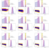 |
Fig. 1. Corner plots of χ2 surface as a function of the model parameters (Δη, ζw) for MAGMA binned by Mstar. The violet contours correspond to the minimum χ2 value. The top and right panels of each corner plot report the probability density distributions for the marginalized parameters; confidence intervals (±1σ) are shown as violet-tinted shaded rectangular regions, and the MLE (PDF median) is shown by a vertical dashed line. |
Figure 1 shows that Δη is degenerate; low values of χ2 can be achieved for a broad range of Δη. However, strikingly, the spread of allowed values for Δη at low Mstar (in the two upper left-most panels in Fig. 1) is much broader than for higher stellar masses. In the higher Mstar bins, the allowed distribution of Δη is truncated to increasingly small values of Δη. This implies that ηa, with equal probability, can be significantly larger than ηw at low masses, as also shown by the PDFs in each panel. Another clear result that emerges from Fig. 1 is that higher ζw occur at lower Mstar.
Figure 1 also shows that while the PDF of ζw shows a form similar to a Gaussian distribution, and is thus fairly well constrained, the PDF for Δη is not. It peaks at a given value, but then falls off toward lower values gradually, leading to the conclusion that the best-fit value may depend on the interval over which the uniform prior is sampled. To investigate this, we have performed the Bayesian calculations using two different intervals in Δη:Δη ∈ [ − 10, 3.4] and Δη ∈ [0, 3.4], again in linearly sampled steps. These cornerplots are shown in Appendix A, and the best-fit values for Δη and ζw for Δη ∈ [0, 3.4] are given in the last two columns of Table 1.
Δη and ζw obtained in bins of mass for Bayesian method.
Results are shown graphically in Fig. 2, where Δη is plotted against Vcirc in the upper panel and ζw vs. Vcirc in the lower one. Because the outflow strengths probably depend on the depth of the potential well, we assess them in terms of the virial velocities, Vcirc, as proposed by Peeples & Shankar (2011). We have calculated virial velocities in several ways, but ultimately adopt Vout, velocities from the baryonic Tully–Fisher relation (BTFR) predicted by APOSTLE/EAGLE simulations from Sales et al. (2017), focused on the low-mass regime. Other alternatives are also viable, such as the power-law BTFR from Lelli et al. (2016b), or velocities obtained from the Mvir − Mstar relation via halo abundance matching (Moster et al. 2010). However, at low Mstar, and low baryonic masses, the inferred virial velocities change significantly according to whether the relation is a straight power law as in Lelli et al. (2016b) or inflected at low masses as in Sales et al. (2017). The simple power-law relation gives Vcirc values that are apparently too low relative to the rest of the sample, while the Vcirc values by Sales et al. (2017) are more consistent. Moreover, because the low-mass end of our sample is somewhat extreme, there is also some doubt about the applicability of the usual halo-abundance matching techniques. In any case, our conclusions are independent of the formulation used to translate the mass scale to the kinematic one.
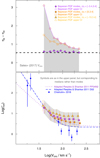 |
Fig. 2. Difference of mass-loading factors Δη (top panel) and metal-loading factors ζw (bottom panel) as a function of virial velocities obtained from the BTFR from Sales et al. (2017). In both panels, filled symbols show the Bayesian results, and in the top panel, open ones illustrate the upper bound of the PDF 1σ confidence intervals (CI). Different symbol types correspond to the interval of Δη in the Bayesian priors, as described in the text; the symbols for Δη ∈ [0, 3.4] and Δη ∈ [ − 10, 3.4] are (arbitrarily) offset along the abscissa for better visibility. The gray regions give the ±1σ uncertainties in the best-fit values. Also shown is the “equilibrium” asymptote, namely Δη = α (see Sect. 3.1). In the top panel, the two estimates of Δη from different priors are exactly coincident. In the bottom panel, the formulations by Peeples & Shankar (2011) for two O/H calibrations, redone here for our value of y, are given by (purple) short-dashed and (blue) long-dashed curves for the PP04N2 and D02 calibrations, respectively. Also shown are the metal-loading factors computed by Chisholm et al. (2018) from COS data. The text gives more details. |
As shown in Fig. 2, the different intervals used for the Bayesian priors give fairly consistent results both for Δη and for ζw. The best-fit Bayesian value for Δη is ≈α for all the prior intervals sampled, and there is a clear trend for ζw to increase toward lower Vcirc (or stellar mass, as we show later). Over the mass range sampled by MAGMA, ζw is almost a factor of ten higher at lower Mstar (Vcirc) relative to the most massive galaxies.
Also shown in the bottom panel of Fig. 2 are the estimates of ζw obtained by Chisholm et al. (2018) with Cosmic Origins Spectrograph (COS) observations of ultraviolet absorption lines. By analyzing the underlying stellar continuum, and using the observed line profiles to constrain optical depth and covering fraction, Chisholm et al. (2018) were able to quantify the mass outflow rate, Ṁw. Then, through photoionization modeling, they obtain column densities of each element that are then used to constrain the metallicity of the outflow Zw. As shown in Chisholm et al. (2018), their results are well fit by the analytical predictions of Peeples & Shankar (2011), with yields in the range 0.007−0.038, which agree with our reference value of y = 0.037.
4.2. Comparison with a closed-form approximation
Figure 2 also illustrates the predictions of Peeples & Shankar (2011) using their formulation for the MZR (taken from Kewley & Ellison 2008, and converted to a Chabrier 2003 IMF). Peeples & Shankar (2011) inferred ζw from the behavior of Mg and Zg with Mstar, using known derivatives derived empirically; we discuss this approach more fully below. Figure 2 shows their formulation relating ζw and Vcirc:
 (22)
(22)
where, for consistency, we have recomputed their fits using our higher adopted yield (for yO) of 0.037 taken from Vincenzo et al. (2016) for a Chabrier (2003) IMF. As shown in Fig. 2, the PP04N2 results are in good agreement with MAGMA, while the D02 calibration (Denicoló et al. 2002) is slightly discrepant, and more consistent with Chisholm et al. (2018), despite the higher yield. This illustrates how the computed ζw values depend on the adopted yields, and underscores the necessity of a self-consistent framework. We have performed our entire metallicity analysis with lower (and higher) yields than the ones used here, and the results do not change.
Peeples & Shankar (2011) assessed Δη and ζw based on known derivatives calculated from observed scaling relations of Mg and Zg with Mstar. In some sense, this is complementary to our Bayesian approach, but may also skew results as we show below. Following Pagel (2009), the time dependence in Eq. (9) can be eliminated by noting that Ṁ⋆ = α ψ. Thus, by changing variables we obtain:
 (23)
(23)
The same can be done for Eq. (10), and eliminating the time dependence as above gives:
 (24)
(24)
Our observations do not directly constrain MZ, but rather Zg, so we need to formulate dZg/dM⋆ as follows:
 (25)
(25)
The left-hand side is given by Eq. (24), and dMg/dM⋆ by Eq. (23), so we can solve for dZg/dM⋆:
![Mathematical equation: $$ \begin{aligned} \frac{\mathrm{d}Z_{\rm g}}{\mathrm{d}M_{\star }} = \frac{1}{\alpha \,M_{\rm g}}\,\left[q + Z_{\rm g}\,(\zeta _{\rm a} - \zeta _{\rm w} - \eta _{\rm a} + \eta _{\rm w})\right]. \end{aligned} $$](/articles/aa/full_html/2022/01/aa40414-21/aa40414-21-eq32.gif) (26)
(26)
As they should be, Eqs. (23) and (26) are related to Eqs. (9) and (12) by the simple derivative, Ṁ⋆ = α ψ. Equations (23) and (26) are slightly different from the ones derived by Peeples & Shankar (2011), because of the different assumptions they made for the stellar enrichment given by Eq. (5).
For a given Mg vs. Mstar relation, we know dMg/dMstar, the left side of Eq. (23); for a given MZR, we know dZg/dMstar, the left side of Eq. (26). Thus, in the spirit of Peeples & Shankar (2011), Δη = ηa − ηw and ζw can be directly constrained observationally. Inverting Eqs. (23) and (26) gives Δη and ζw explicitly:
 (27)
(27)
![Mathematical equation: $$ \begin{aligned}&\zeta _{\rm w} = \frac{q}{Z_{\rm g}}-\alpha \,\left[F_{\rm g}\left(\frac{\mathrm{d}\log Z_{\rm g}}{\mathrm{d}\log M_{\star }} + \frac{\mathrm{d}\log M_{\rm g}}{\mathrm{d}\log M_{\star }}\right)+ 1\right]\nonumber \\&\quad = \frac{q}{Z_{\rm g}}-(\eta _{\rm a}-\eta _{\rm w})-\alpha \,F_{\rm g}\,\frac{\mathrm{d}\log Z_{\rm g}}{\mathrm{d}\log M_{\star }}\cdot \end{aligned} $$](/articles/aa/full_html/2022/01/aa40414-21/aa40414-21-eq34.gif) (28)
(28)
In Eq. (28), we have defined Fg ≡ Mg/Mstar. Peeples & Shankar (2011) were the first to derive such a formulation for ζw; as mentioned in Sect. 3, the formalism here differs slightly from theirs because of the way they dealt with metal production in stellar ejecta.
The problem with Eq. (27) is that for positive d log Mg/d log Mstar, Δη is by definition > 0, because Fg is ≥0. In Paper II, the robust least-squares power–law relation5 between Mg and Mstar is found to be:
 (29)
(29)
thus with d log Mg/d log Mstar ≈ 0.7, roughly consistent with earlier works (e.g., Leroy et al. 2008). Because of this positive derivative, to infer Δη by relying on Eq. (27) and d log Mg/d log Mstar would give results that are inherently skewed toward higher values of Δη. Qualitatively, we would expect that as a galaxy evolves, the stellar mass continues to grow, while the gas mass diminishes; such a scenario would give d log Mg/d log Mstar < 0, and possibly Δη < α. Consequently, from a physical point of view, it may be inaccurate or unrealistic to invoke the sample’s overall d log Mg/d log Mstar to calculate Δη. What we require is an estimate of Δη for individual galaxies which may or may not be related to the statistical properties of the parent sample at z ≈ 0.
In any case, Fig. 2 illustrates that ζw is not particularly sensitive to Δη. The predictions of ζw from Peeples & Shankar (2011) using d log Mg/d log Mstar are fairly consistent with those we find with the Bayesian approach, even though the former requires Δη > 0 and the latter suggests that Δη ≈ 0.
5. Shaping the mass–metallicity relation with outflows
In the previous section, we estimated Δη and ζw through a Bayesian approach. Here we parameterize Δη and ζw as a function of both Mstar and μg to predict quantitatively how mass loading Δη and metal loading ζw shape the MZR.
5.1. Stellar mass, metallicity, and outflows
First, we incorporate Mstar as the defining variable. Figure 3 (left panel) shows the trends of Bayesian-inferred Δη and ζw with observed Zg as a function of Mstar (in logarithmic space). The bottom left panel shows the predictions for Zg that are inferred from the functional forms we have found for Δη and ζw (see Table 2). The middle left panel shows ζw together with the robust cubic best-fit polynomials with coefficients as given in Table 2. The cubic polynomial has no physical significance; rather our objective is to parameterize Δη and ζw relative to Mstar in order to compute Zg.
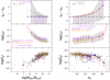 |
Fig. 3. Difference of mass-loading factors Δη and metal-loading factors ζw inferred from the Bayesian analysis, and observed Zg in the bottom panel, as a function of Mstar on the left, and as a function of μg on the right. In the two upper panels, the best-fit Bayesian values are shown as filled symbols (circles or squares according to the Δη prior), with error bars corresponding to the ±1σ excursion, which is also illustrated by light-gray shaded regions. The rightmost point (magenta circle) in the top and middle right panels corresponds to the “extra” high-μg bin shown in Fig. 6. In the top panels, a horizontal dashed line illustrates the “equilibrium solution” with Δη = α. In the top left panel, the (purple) dashed curve is a linear power-law fit of Δη to log(Mstar), while the dashed curve in the top right panel shows Eq. (27), with d log Mg/d log Mstar = 0.72, as found in Paper II. The fits to the curves for ζw in the middle panels are cubic: log(ζw) as a function of log(Mstar) in the left panel, and ζw as a function of Fg in the right. In the lower panels, observed MAGMA Zg are shown as small filled circles, color coded by gas fraction, while the Zg medians and 1σ deviations are shown by large (black) filled circles and error bars. The dashed curves in the lower panels correspond to the calculation of Zg based on the fits in the upper panels (as a function of μg on the left, and log(Mstar) on the right): the long-dashed curves (dark orange) correspond to the Δη ≥ 0 priors, while the short-dashed ones (purple) to the “symmetric” priors. The green curves in the left panels are described in the text, obtained by fitting individual galaxy Δη and ζw calculated using Eqs. (27) and (28). |
Robust polynomial fits to Bayesian estimates of Δη and ζw.
The slight differences (∼0.15 dex for Mstar ≳ 109 M⊙, long-dashed orange- vs. short-dashed purple curves) in ζw according to the Δη prior are evident in the middle left panel in Fig. 3 and the lower one. When the constraint on the prior Δη > 0, the Bayesian inference of ζw gives lower values, and is a better approximation of observed Zg (orange long-dashed curve). On the other hand, when the Δη priors include negative values ζw is larger (see also Fig. 2), but Zg is underestimated (purple short-dashed curve). Since the curves shown in the lower panel are not fits to Zg, but rather the parameterization of Zg as a function of Δη and ζw, this may be telling us that positive values over negative Δη are preferred, at least in the current evolutionary states of the MAGMA galaxies.
The green curves in the top two left panels of Fig. 3 illustrate the polynomial fits (quadratic for Δη and cubic for log ζw) that would be obtained had we calculated Δη and ζw from Eqs. (27) and (28), respectively, using d log Zg/d log M⋆ and d log Mg/d log M⋆ derived from the MAGMA scaling relations. The corresponding green curve in the lower left panel is the approximation of Zg that would be obtained from these fits. It is clear that for log Mstar/M⊙ ≳ 8.5, Zg is equally well estimated by the priors of Δη ≥ 0 and the fits to individual parameters computed with Eqs. (27) and (28). Wind metal loading ζw estimated with the symmetric prior of Δη falls short (∼0.15 dex) of observed Zg in this mass range. In this mass range, Fig. 3 also shows that Δη is unimportant; the main factor that shapes Zg is ζw.
On the other hand, the fit to Δη in the top panel (green curve, Eq. (27)) is significantly rising toward lower Mstar, unlike the Bayesian values for Δη that, with both sets of priors, is roughly constant ≈α. The influence of Δη at low Mstar (log Mstar/M⊙ ≲ 8.5) is clearly shown by the green curve in the lower left panel of Fig. 3. The fall-off of Zg toward low Mstar is less severe than would be predicted by a flat Δη, and is more consistent with the observations.
5.2. Gas fraction, metallicity, and outflows
In Paper II (see also Eq. (29)), we found that gas content Fg grows with decreasing stellar mass (see also e.g., Haynes et al. 2011; Huang et al. 2012; Boselli et al. 2014b; Saintonge et al. 2017; Catinella et al. 2018). Figure 4 shows this comparison explicitly for baryonic gas fraction μg and Mstar in MAGMA galaxies. There is a clear trend for higher μg as Mstar decreases, but in the very lowest Mstar regime, below log(Mstar/M⊙) ≲ 8.5, the scatter is large. In MAGMA, most galaxies in this regime have μg ≳ 0.5, but there are two exceptions, Sextans A and WLM, at very low μg despite low global stellar mass. This apparent inconsistency probably arises from underestimates of the total gas content corresponding to the localized regions where CO was detected (e.g., Shi et al. 2015, 2016; Elmegreen et al. 2013; Rubio et al. 2015), and indicates the inherent difficulties of probing the gas, stellar, and metal contents in these extreme dwarf systems. Although the median trend for less-massive galaxies to be more gas rich is evident down to Mstar ∼ 3 × 10⁸ M⊙, the large overall scatter makes it virtually impossible to infer trends of Δη and ζw with μg from their trends with Mstar.
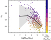 |
Fig. 4. Baryonic gas fraction μg plotted against (log) Mstar for MAGMA galaxies. Galaxies are coded by gas fraction, Fg, as shown in the vertical color bar. MAGMA medians are shown as a heavy gray line, with ±1σ excursions as the gray region. As noted in the text, the two low-mass galaxies with low μg are Sextans A and WLM, with probable substantial underestimates of the total gas content. |
Thus, to assess the dependence of Δη and ζw on μg, we cannot use the analysis of Sect. 4.1. Consequently, we repeated the Bayesian estimation by binning in μg, rather than in Mstar. As before, bin boundaries were chosen such that a similar number of galaxies is found in each of the nine bins; the priors for Δη and ζw are as before (see Sect. 4.1). The results for the symmetric prior on Δη ∈ [ − 3.4, 3.4] are shown in Fig. 5, where the layout of the figure is the same as in Fig. 1. Here there is a trend for larger Δη excursions at high μg (see lower panels), similar to what we found for low Mstar. There is also a tendency for the distribution of ζw to be broader at high μg, that is also reflected in the broader range of Δη.
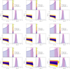 |
Fig. 5. Corner plots of χ2 surface as a function of the model parameters (Δη, ζw) for MAGMA binned by μg. The violet contours correspond to the minimum χ2 value. The top and right panels of each corner plot report the probability density distributions for the marginalized parameters; confidence intervals (±1σ) are shown as violet-tinted shaded rectangular regions, and the MLE (PDF mode for Δη, median for ζw) is shown by a vertical dashed line. |
At high μg, there is some evidence for a bimodal distribution of ζw, as shown in Fig. 6, where we have raised the boundary of the highest μg bin. In this μg bin, the rightmost one plotted in Fig. 5, the best-fit (mode) Δη is higher than any. Nevertheless, as can be seen in the lower-right panel, higher values of ζw are possible for virtually every Δη sampled, so that the dependence of ζw on Δη is apparently degenerate, as we concluded in Sect. 4.1.
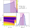 |
Fig. 6. Corner plot of χ2 surface as a function of the model parameters (Δη, ζw) for the highest μg bin MAGMA, here with a higher boundary than in Fig. 5: μg > 0.75. As in previous figures, the violet contours correspond to the minimum χ2 value, and the top and right panels report the probability density distributions for the marginalized parameters. Confidence intervals (±1σ) are shown as violet-tinted shaded rectangular regions, and the MLE (PDF mode for Δη, median for ζw) is shown by a vertical dashed line. |
To parameterize Δη and ζw, here we adopt Fg as the independent variable because it is statistically better behaved than μg, as a result of the simpler dependence on Mstar. However, it is more convenient to compare quantities to μg as shown in the right panel of Fig. 3 where Bayesian estimates for Δη, ζw, and observed Zg are plotted as a function of μg. The curve in the top right panel is not a fit, but rather the prediction of Eq. (27) using d log Mg/d log Mstar = 0.72 from Eq. (29). The middle right panel shows ζw together with the robust cubic best-fit polynomial with coefficients as given in Table 2. Metallicity vs. μg is given in the bottom right panel, where the long-dashed curve corresponds not to a fit, but rather to the prediction of Eq. (15) with the functional forms for ζw (cubic polynomial) and Δη. The difference in ζw for the two different priors for Δη in the Bayesian analysis are analogous to those for Mstar (left panel Fig. 3). At low μg, Zg is better approximated by ζw inferred from Δη > 0 relative to ζw from the symmetric prior.
The influences of ζw and Δη are clearly seen in the trend for Zg with μg. The steep increase of ζw and Δη toward high μg is reflected in the dramatic reduction of metallicity toward high μg. The shape of the MAGMA Zg curve relative to μg resembles that found by Erb (2008, see her Fig. 3), for z ∼ 2 galaxies, but with some important differences. The first is that Erb (2008) assume that Zw/Zg = 1, that is to say that ζw = ηw. Appendix C presents the trivial derivation of this result. Under this assumption, Zg in Eq. (15) is essentially governed by ηa, with ηw entering only into the Mg/Mi exponent (see also Appendix C). Consequently, there is less variation at low μg, with the prediction by Erb (2008) assuming a constant asymptotic value for μg as high as ∼0.35. By considering the change in Zw relative to Zg, as we do here, Zg never reaches a truly asymptotic value, although there is flattening toward lower μg.
The second difference is the assumption for R (thus α) in the metallicity treatment of Erb (2008). She uses the same metallicity calibration as adopted here (PP04N2), but assumes that α, the fraction of gas retained in stars, is unity, thus neglecting the gas that is expelled in SNe and stellar winds. This would imply a difference −0.34 dex in her and our absolute metallicity scale. An additional factor is the different yield adopted here (y = 0.037) relative to y = 0.019 used by Erb (2008). Considering these two numerical differences, the absolute scale in Erb (2008) would be reduced by ∼0.6 dex. Such a difference is consistent with the galaxies shown by Erb (2008), considering that her sample is at z ∼ 2, while MAGMA is at z ∼ 0. Thus, as observed, lower Zg (∼ − 2.7 dex) at low gas fractions would be expected for her sample relative to ours (e.g., Erb et al. 2006; Maiolino et al. 2008).
5.3. Considerations
Interpretation of our results is not altogether straightforward. On the one hand, the Bayesian analysis shows that Δη as a function of Mstar tends toward α which would indicate a condition of “gas equilibrium” (e.g., Davé et al. 2012; Mitra et al. 2015). On the other, Δη as a function of μg does not show this behavior, but rather resembles what would be predicted by Eq. (27). This distinction stems from the highly imperfect correlation of μg with Mstar as shown in Fig. 4. Figures 1 and 5 also illustrate that a wide range of Δη is possible (Δη < 0, Δη < α, Δη ≥ α), but that this only weakly affects ζw.
Our analysis also shows that within a 1σ range, Δη can be < α, over all mass ranges, but possibly more importantly, Δη can be significantly > α toward low Mstar and high μg (see Fig. 3). We take this to imply that at low Mstar and high μg there is more possibility for increased overall gas accretion (ηa) relative to wind outflows (ηw). This could be related to the stochastic nature of star-formation histories in low-mass galaxies (e.g., Weisz et al. 2012; Madau et al. 2014; Krumholz et al. 2015; Emami et al. 2019), and to the availability of gas.
Figure 3 shows that Δη ≈ α almost independently of Mstar, thus implying gas equilibrium at all masses; however, Δη increases as a function of μg roughly as predicted by Eq. (27). Because we would expect that younger, less evolved, galaxies contain more gas, thus higher μg, this would seem to suggest that Δη could depend on the evolutionary phase of a galaxy. Since we cannot know the star-formation histories (SFHs) of the individual galaxies, this suggestion is difficult to test. However, we can fix a simple SFH, such as a falling or rising exponential, and experiment with what such a “toy model” would predict for d log Mg/d log Mstar as a function of time. If we consider that the timescale of star formation τSF is tightly linked to the gas depletion time τg ( ), we can explicitly calculate the growth of Mstar and Mg using Eqs. (2) and (14), respectively.
These toy-model calculations are shown in Appendix B. As expected, d log Mg/d log Mstar depends clearly on Δη; both positive and negative values of d log Mg/d log Mstar are possible depending on the SFH, the age of the galaxy tgal, the timescale for star formation τSF, and most importantly on Δη. The value of Δη, relative to α in the exponent of Eq. (14), determines whether gas mass is increasing or diminishing with time. Since stellar mass is monotonically increasing, the value of Δη sets the value of d log Mg/d log Mstar. Nevertheless, our results show that Δη is almost impossible to constrain, demonstrating behavior that varies according to whether the independent variable is Mstar or gas content μg.
As discussed in Sect. 3.2, when Δη = α, as for the “gas-equilibrium” scenario, Eq. (15) is numerically intractable because of the zero denominator in the exponent for Mg/Mi. This same condition gives Ṁg = 0 and Mg = Mi (see Eq. (16)). Because of the relatively long total-gas depletion times, ∼a few Gyr, even without a true equilibrium solution, essentially Mg/Mi remains unity throughout most of the lifetime of the galaxy (see Eq. (14)).
An important aspect of our formalism is that, in essence, through Eq. (13), we assume that the SFH corresponds also to the time evolution of gas mass. Moreover, because we assume that total system mass is conserved and that the time derivative of accreted gas mass Ṁa is proportional to SFR through ηa, it is possible that the formalism itself requires a rough equality between Δη and α, the lock-up fraction.
Despite the degeneracy of Δη and the inability of our formalism to determine unambiguously its behavior, ζw is fairly well determined (see Figs. 2 and 3). After discussing effective yields in Sect. 6, in the remainder of the paper, we focus on ζw, and what can be learned from our results about metal- and mass-loading in the stellar-driven outflows of star-forming galaxies.
6. Effective yields
Above we have quantified a scenario for the relation between Zg and gas content in galaxies that requires significant gas accretion and stellar-driven outflows. In this section, we recast our results in the context of the effective yield, as measured against the predictions from a different, “closed-box”, paradigm. A galaxy evolving as a closed box obeys a simple relationship between the metallicity and the gas mass fraction (Searle & Sargent 1972; Pagel & Patchett 1975):
 (30)
(30)
where μg is the baryonic gas mass fraction and y is defined as the “true” yield (Sect. 3.1). As gas is converted into stars, metal content grows and the gas mass diminishes. If the galaxy evolves as a closed box, then the yield y in Eq. (30) should be equal to the nucleosynthetic yield. However, galaxies do not evolve as closed systems, so we expect the overall metal yield to differ from the nucleosynthetic value. The effective yield yeff can be defined by inverting Eq. (30) (e.g., Lequeux et al. 1979):
 (31)
(31)
The effective yield is expected to be lower than the nucleosynthetic value y because metals in galaxies are lost from the system through outflows, and the metal content of the ISM gas will be diluted with infall of metal-poor gas (e.g., Edmunds 1990).
The effective yields yeff for MAGMA, computed using Eq. (31), are shown in Fig. 7, plotted against baryonic gas mass fraction μg. The model prediction from Eq. (15) through our parameterizations of Δη and ζw is shown as two curves, corresponding to the two different Δη priors. For reference, our adopted value of y is shown as a horizontal short-dashed line. As also evident in previous figures, the results from the Δη ≥ 0 prior (long-dashed orange curve) are in slightly better agreement with the data. The inflection of yeff at high μg is due mainly to the strong downward curvature of Zg as seen in Fig. 3. Moreover, yeff is always (with a single possible exception at high μg, NGC 4731) significantly smaller than the true yield y = 0.037 adopted here. Edmunds (1990) has shown that this behavior for yeff would be expected if metals were lost through stellar- and SNe-driven bulk outflows, or diluted by accretion of metal-poor gas. MAGMA shows a strong confirmation of this scenario. It is clear from Fig. 7 that our parameterized model is a good approximation to the data (see also Fig. 3).
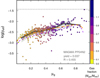 |
Fig. 7. Effective yield as a function of μg. Galaxies are coded by gas fraction, Fg, as shown in the vertical color bar. MAGMA medians are shown as a heavy gray line, with ±1σ excursions as the surrounding gray regions. The two dashed curves correspond to the predictions from the Δη and ζw parameterizations (see also Fig. 3), with the symmetric Δη priors given as a short-dashed (purple) curve, and the Δη ≥ 0 priors as a long-dashed (orange) one. The horizontal dashed line corresponds to our adopted true yield y = 0.037 (see text). |
Models that do not take into account the metal-enriched bulk outflows at low Mstar, namely assuming that Zw = Zg, predict that at high μg, yeff would approach the nucleosynthetic value y (e.g., Erb 2008). This can be seen by expanding Eq. (31) in a Taylor’s series (see Dalcanton 2007; Filho et al. 2013) so that for high μg, we have:
 (32)
(32)
Thus, in very gas-rich galaxies, the effective yield would be approximately independent of gas fraction. As pointed out by Dalcanton (2007), metal-poor accreted gas will lower the metallicity of the system, but it will also augment μg, thus maintaining the system in a pseudo-closed-box equilibrium. The linear dependence of yeff on metal mass MZ, as shown by Eq. (32), also means that metal-enriched outflows are very effective at lowering the effective yield in galaxies with high gas-mass fractions (see Dalcanton 2007). Indeed, Fig. 7 shows that even at high μg, yeff is significantly lower than the true yield y.
It is important to remember that Eq. (31) measures Zg in the ionized gas, but the gas content μg is derived from neutral gas (H I + H2). There is some evidence that the metal contents of these two gas phases are different; in UV absorption studies of metal-poor dwarf galaxies (e.g., Thuan et al. 2005; Lebouteiller et al. 2013), the metallicity of the neutral gas in these systems was always found to be lower than in the ionized gas. A similar conclusion was reached by Filho et al. (2013) and Thuan et al. (2016) by comparing yeff with y, and attributing the difference to the lower metallicity in the neutral gas.
Figure 8 plots the effective yield yeff against stellar mass Mstar (left panel) and circular velocity, Vcirc (right). Even though there is much scatter at low Mstar and Vcirc (Mstar ≲ 3 × 10⁸ M⊙ and Vcirc ≲ 50 km s−1), yeff is increasing with mass and velocity up to 3 × 10⁹ M⊙ and ∼100 km s−1, in qualitative agreement with similar trends reported in the literature (e.g., Garnett 2002; Pilyugin et al. 2004; Tremonti et al. 2004; Dalcanton 2007; Ekta & Chengalur 2010). For more massive galaxies, there is an inflection in the relations with a mild decline at masses and velocities larger than 3 × 10⁹ M⊙ and ∼100 km s−1.
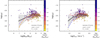 |
Fig. 8. Effective yield as a function of Mstar (left panel) and Vcirc (right panel). Galaxies are coded by gas fraction, Fg, as shown in the vertical color bar. MAGMA medians are shown as a heavy gray line, with ±1σ excursions as the surrounding gray regions. Also shown in the left panel as two dashed curves are the predictions from the Δη and ζw parameterizations (see also Fig. 3), with the symmetric Δη priors given as a short-dashed (purple) curve, and the Δη ≥ 0 priors as a long-dashed (orange) one. The right panel illustrates galaxies with high star-formation efficiency (short gas depletion times) with a blue dashed curve, and those with low efficiency (long depletion times) as a red one. The horizontal short-dashed line corresponds to the yield of 0.037 adopted in this paper. See text for more details. |
The right panel of Fig. 8 also shows the MAGMA sample divided into two regimes in gas depletion times, τg, defined as Mg/SFR (see Paper II); galaxies with long τg (τg > 4 × 10⁹ yr) are shown as a dashed red curve, and short times τg < 4 × 10⁹ yr as a dashed blue one. The gas depletion time τg is the inverse of the so-called star-formation efficiency (SFE, see Paper II), that also enters into Eq. (13), so short τg would correspond to higher SFE, and vice versa. There can be as much as a factor of ten in yeff between these two categories of galaxies, with a mean difference of ∼2 − 3 in yeff. At fixed mass, larger yields correspond to longer τg or lower SFE. In these galaxies with longer τg, the peak in yeff at Mstar ∼ 3 × 10⁹ M⊙ seems to disappear, while there is a steady decline of yeff toward lower Mstar for shorter depletion times (see also Lara-López et al. 2019). Longer τg are also associated with higher gas fractions (see color coding in Fig. 8); thus Eq. (32) may be telling us that the higher effective yields are simply a function of the enhanced impact of metal-enriched outflows in gas-rich galaxies.
7. Characterizing stellar feedback through winds
By adopting the formalism for galactic chemical evolution formulated by Pagel (2009), we have quantified with MAGMA the metal-weighted mass loading factor ζw (=ηwZw/Zg), and with somewhat less success, the difference in mass loading of gas accretion and outflows, Δη. However, we are interested in the individual mass-loading factor relative to the SFR, ηw, and the metal content of the winds, Zw. In this section, we explore the constraints for mass loading ηw and Zw provided by our results.
7.1. The entrainment fraction
Assuming that Zw = Zg, as done in much previous work (e.g., Erb 2008; Finlator & Davé 2008; Dayal et al. 2013; Hunt et al. 2016; Belfiore et al. 2019), implies that virtually all of the material in the outflow is ISM gas. The gas metallicity could be only a lower limit to the metallicity of the wind (e.g., Peeples & Shankar 2011), because the metals produced by SNe would be expected to enrich the gas above that of the galaxy (e.g., Vader 1986). Thus, to estimate Zw, we also need to consider the fraction of gas that has been entrained in the wind, fent, and the metallicity of the SNe ejecta, Zeject (see Dalcanton 2007; Peeples & Shankar 2011):
 (33)
(33)
In low-mass galaxies, fent is found to be low, both observationally (e.g., Martin et al. 2002) and from simulations (e.g., Mac Low & Ferrara 1999). The entrainment fraction is closely related to the mass-loading factor of the wind ηw, and probably varies with galaxy mass (gravitational potential, see e.g., Hopkins et al. 2012). The maximum oxygen abundance of SNe ejecta Zeject is known to within a factor of 2−3, Zeject ∼ 0.04 − 0.1 (e.g., Woosley & Weaver 1995), and can constrain fent and ηw (e.g., Martin et al. 2002). The increase of ζw with decreasing virial velocity and stellar mass (see Fig. 2) is possibly due to diminishing fent to raise Zw closer to Zeject. To verify this, we need to isolate ηw, the mass-loading factor in the product ζw = ηwZw/Zg.
7.2. The driving mechanisms behind stellar outflows
One way to do this is to compare the Vcirc scaling of ζw with expected Vcirc scalings of ηw (see Eq. (22)). Galactic outflows powered by stellar feedback are thought to be driven either by momentum, imparted to the ISM by massive stellar winds and SNe through radiation pressure (e.g., Murray et al. 2005, 2010; Hopkins et al. 2011; Zhang & Thompson 2012), or by energy, injected into the ISM by massive stars and core-collapse SNe (e.g., Dekel & Silk 1986; Heckman et al. 1990; Dalla Vecchia & Schaye 2012; Christensen et al. 2016; Naab & Ostriker 2017).
For outflows that conserve momentum, we would expect a power-law scaling  while for energy-conserving winds,
  (e.g., Dekel & Silk 1986; Murray et al. 2005; Hopkins et al. 2012). The only way such scalings can be reconciled with the (modified power-law) form of Eq. (22) is by a complementary scaling of Zw. Examples of such complementary scaling are shown in Fig. 9 where the ratio of wind and ISM metallicities Zw and Zg is plotted against virial velocity Vcirc. In the left panel of Fig. 9, we have taken the normalization of Zw/Zg to be the same as that as the best-fit of Eq. (22) using our Bayesian estimates, simply Vcirc/V0, where V0 = 32 km s−1 for symmetric Δη priors, and V0 = 35 km s−1 for priors with Δη ≥ 0. Both fits have power-law index b ∼ 2. The assumptions of momentum-conserving or energy-conserving outflows lead to different estimates for the trend of Zw/Zg.
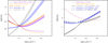 |
Fig. 9. Ratio of inferred wind and ISM metallicities Zw/Zg plotted against virial velocity Vcirc. Also shown (with arbitrary scaling) is the shape of Bayesian ζw as also plotted in Fig. 2; it is clearly not a power law, thus the different power-law forms of ηw introduce inflections in Zw/Zg. Left panel: as indicated in the legend, different trends of Zw/Zg are inferred by dividing the fitted form of ζw (see Eq. (22)) by various scalings of ηw (see text for more details). The shaded regions correspond to the trends allowed by the two different Bayesian estimates of ζw according to the different Δη priors. Right panel: broken-power law trend for ηw found by Muratov et al. (2015) is shown as a solid heavy (gray) curve, where the inflection at Vcirc = 60 km s−1 corresponds to a sharp decrease of Zw/Zg (see text for more details). The short-dashed (dark-blue) curve shows the relation found by Mitchell et al. (2020), in the low-mass regime where stellar feedback dominates, and the long-dashed (blue) curve shows the observed relation derived by Chisholm et al. (2018). |
Because dwarf galaxies are found to have a low entrainment fraction (e.g., Mac Low & Ferrara 1999; Martin et al. 2002), we would expect Zw/Zg to increase toward low Vcirc because low fent would enrich the outflows toward the higher super-Solar abundance of the SNe ejecta, Zeject (see Eq. (33)). Energy-conserving winds result in a flattening of Zw/Zg toward low Vcirc (blue curves), and a cubic trend of ηw with Vcirc gives a strongly declining Zw/Zg (gray curves). The trend of  is the only one that gives a rising trend of Zw/Zg at low Vcirc. Thus, momentum-conserving winds would be favored by our results.
Quantifying this conclusion is, however, dependent on the metallicity calibration. For the PP04N2 calibration used here, the roughly quadratic low-mass Vcirc dependence is shallower than the cubic (or quartic) dependence found by Peeples & Shankar (2011) for different O/H calibrations. Other calibrations such as those by Tremonti et al. (2004) or Denicoló et al. (2002) give differing trends (with power-law slopes b > 3 at low Vcirc), that are inconclusive for determining the nature of the mass-loading factor ηw. The PP04N2 calibration adopted here results in the shallowest increase of ζw toward low Vcirc (power-law slope b ≈ 2), relative to other O/H calibrations, and this is reflected in a more incisive low-mass (low Vcirc) increase in Zw/Zg.
The right panel of Fig. 9 shows the predictions for ηw from the sub-grid FIRE (Feedback in Realistic Environments) simulations (Muratov et al. 2015), and the EAGLE simulations (Mitchell et al. 2020). At low Vcirc (< 60 km s−1), Muratov et al. (2015) find the power-law dependence on Vcirc to be steep (∼ − 3.2), while at higher masses (Vcirc) the winds are momentum-driven with ηw ∝  . A similar conclusion was reached by Davé et al. (2013), namely that at low masses, winds are energy-driven (or even more steeply with Vcirc), while momentum-driven winds dominate at higher masses. Judging from Fig. 9, these trends would be incompatible with our results. In contrast, EAGLE simulations (e.g., Mitchell et al. 2020) indicate a slope midway between, namely ∼ − 1.5, leading to a very gradual increase in metallicities toward lower Vcirc. Comparing the left- and right-hand sides of Fig. 9 shows that such a dependence better reflects our results at low Vcirc. At higher Vcirc (masses), the situation is more complex because the flattening of ζw is difficult to interpret in terms of a single power-law dependence of ηw on Vcirc. In any case, we conclude that at low masses, winds in stellar outflows cannot be energy driven, but rather are more consistent with momentum-driven outflows (
 ), or a slightly steeper “combined” slope as found by the EAGLE models with
  .
.
There is also the question, not touched upon here, of whether or not outflows are able to expel material from the galaxy halo, thus enriching the IGM. The entrainment fraction fent would be key to relating the strength of the outflows with metallicity in the winds (e.g., Martin et al. 2002; Chisholm et al. 2018) and deserves further study. In addition, entrainment is also affected by the gas phases involved in the outflow. Our analysis traces the metallicity in the ionized gas (considered the “cool” phase by most simulations, T < 2 × 10⁴ K), thought to carry most of the mass, whereas physically realistic winds also contain a “hot phase” (T > 5 × 10⁵ K) that harbors most of the energy (Kim et al. 2020). Consequently, with MAGMA, we are missing the diagnostic of the hot X-ray phase.
8. Summary and future perspectives
In this paper, we explore the impact of ejective feedback on galaxy evolution using data from the MAGMA sample of 392 galaxies with H I and CO detections, which collects a homogeneous sample of local field star-forming galaxies, covering the widest range of stellar and gas masses, metalliticies and star formation compiled up to now. After presenting the sample, and the correlations among metallicity, SFR, Mstar and (cool) gas-phase components in Paper I and Paper II, in this third paper of the series, we investigate outflow metal loading factors and effective yields in terms of gas fraction, mass and circular velocity, using the formalism of Pagel (2009). The main results of the paper follow.
-
We model the chemical enrichment of MAGMA galaxies using a formalism based on Pagel (2009), without any constraint on the Mg time evolution and including the assumption that wind metallicity Zw is different from the ISM metallicity Zg. Wind metallicity Zw can be greater than the ambient Zg if it is primarily comprised of supernova ejecta or depressed if a sufficient amount of metal-poor gas is entrained as the wind propagates out of the galaxy (Chisholm et al. 2015; Creasey et al. 2015; Muratov et al. 2017; Pillepich et al. 2018). Using this formalism we have observationally constrained two parameters important for stellar feedback: (a) the metal-loading factor of the winds ζw; and (b) the difference of the mass loading of the accretion and winds, Δη = ηa − ηw. This is done through a Bayesian approach applied to subsamples of galaxies in different Mstar and μg bins.
-
In terms of trends with Mstar, we find that Δη is degenerate, and exceedingly difficult to constrain. However, our Bayesian estimates based on μg bins show that Δη increases significantly with increasing gas fraction, implying that Δη is a strong function of gas content and possibly evolutionary state (see Appendix B).
-
The wind metal-loading factors ζw are found to increase with decreasing stellar mass and circular velocity, with a flattening toward larger Mstar. This indicates that the efficiency of metal-loading in the winds depends on the potential depth and is strongly enhanced in low-mass systems, in agreement with previous work based on different methodologies for estimating ζw (e.g., Peeples & Shankar 2011; Chisholm et al. 2018).
-
We have also constrained effective yields yeff with MAGMA data, and find that yeff increases with stellar mass and Vcirc up to a certain threshold, followed by a flattening toward larger Mstar, and possibly a mild inversion at the highest masses.
-
Finally, we have inferred possible trends with Vcirc for the wind mass-loading factors ηw and find that our results for low Vcirc (Mstar) favor momentum-driven winds, rather than energy-driven ones.
Various quantities in our analysis, ζw, yeff, and Zg, present inflections at Mstar ∼ 3 × 10⁹ M⊙, corresponding to virial velocities ∼100 km s−1. This corresponds to a “gas-richness” mass scale, associated with transitions of physical processes, separating two different mass regimes (Paper II; see also Kannappan 2004). It delineates an accretion-dominated regime at low masses, where stellar outflows are relevant, and an intermediate mass, gas-equilibrium regime, where outflows are less effective, and galaxies are able to consume gas through SF as fast as it is accreted. There would also be an additional, larger “bimodality” mass threshold at Mstar ∼ 3 × 10¹⁰ M⊙ (Paper II, Kannappan et al. 2013) but this is only weakly evident in MAGMA, mainly because of the exclusion of passive or “quenched” gas-poor galaxies and AGN.
These results can also be interpreted within a broader context, since the mass thresholds defining metallicity and gas properties are associated with changes of correlations involving stellar populations and stellar and dark matter distributions (Tortora et al. 2010, 2019). In particular, inflections with mass of metal-loading and metal yields at the “gas-richness” threshold seem to define changes of the slopes of total mass density profiles including dark matter (e.g., Tortora et al. 2019); this threshold approximatively separates galaxies with mass density slopes shallower and steeper than ∼ − 1 (see their Fig. 1). More investigations on this mass scale will follow.
As outlined in Paper II, further improvement of the MAGMA coverage, with more detections of total gas content in dwarf galaxies, will strengthen the conclusions of our series of papers. In addition, it is important to reassess the impact on our conclusions of assumptions made here, namely that the accretion rate Ṁa is proportional to the SFR and the chemically unenriched nature of the accreted gas. In this paper, we have also pursued a first step to combine information from completely independent datasets and observables. Only by including gas, stellar, kinematical and dynamical observables, will we be able to determine the efficiency of the physical phenomena which shape and regulate galaxy evolution.
We do not imply here that the environment does not play a role in baryonic cycling, on the contrary, the idea is that the environment can drive processes that take place within the galaxy, so that ultimately they can be considered “internal”.
Here we are interested in star-forming galaxies only, and do not discuss the effects of AGN feedback on massive galaxies.
This is not particularly computationally tedious because we have a few tens of galaxies within each mass bin, and only two parameters to determine.
For all statistical analysis, we rely on the R statistical package: R Core Team (2018), R: A language and environment for statistical computing, R Foundation for Statistical Computing, Vienna, Austria (https://www.R-project.org/).
Acknowledgments
We thank the anonymous referee and the editor for profound insight that helped to greatly improve the paper. We are grateful for funding from the INAF PRIN-SKA 2017 program 1.05.01.88.04.
References
- Andrews, B. H., & Martini, P. 2013, ApJ, 765, 140 [NASA ADS] [CrossRef] [Google Scholar]
- Baldwin, J. A., Phillips, M. M., & Terlevich, R. 1981, PASP, 93, 5 [Google Scholar]
- Behroozi, P. S., Wechsler, R. H., & Conroy, C. 2013, ApJ, 770, 57 [NASA ADS] [CrossRef] [Google Scholar]
- Belfiore, F., Vincenzo, F., Maiolino, R., & Matteucci, F. 2019, MNRAS, 487, 456 [NASA ADS] [CrossRef] [Google Scholar]
- Boselli, A., Boissier, S., Cortese, L., et al. 2009, ApJ, 706, 1527 [Google Scholar]
- Boselli, A., Cortese, L., & Boquien, M. 2014a, A&A, 564, A65 [NASA ADS] [CrossRef] [EDP Sciences] [Google Scholar]
- Boselli, A., Cortese, L., Boquien, M., et al. 2014b, A&A, 564, A66 [NASA ADS] [CrossRef] [EDP Sciences] [Google Scholar]
- Brinchmann, J., Charlot, S., White, S. D. M., et al. 2004, MNRAS, 351, 1151 [Google Scholar]
- Catinella, B., Saintonge, A., Janowiecki, S., et al. 2018, MNRAS, 476, 875 [NASA ADS] [CrossRef] [Google Scholar]
- Chabrier, G. 2003, PASP, 115, 763 [Google Scholar]
- Chisholm, J., Tremonti, C. A., Leitherer, C., et al. 2015, ApJ, 811, 149 [NASA ADS] [CrossRef] [Google Scholar]
- Chisholm, J., Tremonti, C., & Leitherer, C. 2018, MNRAS, 481, 1690 [NASA ADS] [CrossRef] [Google Scholar]
- Christensen, C. R., Davé, R., Governato, F., et al. 2016, ApJ, 824, 57 [CrossRef] [Google Scholar]
- Creasey, P., Theuns, T., & Bower, R. G. 2015, MNRAS, 446, 2125 [CrossRef] [Google Scholar]
- Dalcanton, J. J. 2007, ApJ, 658, 941 [CrossRef] [Google Scholar]
- Dalla Vecchia, C., & Schaye, J. 2012, MNRAS, 426, 140 [NASA ADS] [CrossRef] [Google Scholar]
- Davé, R., Finlator, K., & Oppenheimer, B. D. 2012, MNRAS, 421, 98 [Google Scholar]
- Davé, R., Katz, N., Oppenheimer, B. D., Kollmeier, J. A., & Weinberg, D. H. 2013, MNRAS, 434, 2645 [CrossRef] [Google Scholar]
- Dayal, P., Ferrara, A., & Dunlop, J. S. 2013, MNRAS, 430, 2891 [Google Scholar]
- Dekel, A., & Birnboim, Y. 2006, MNRAS, 368, 2 [NASA ADS] [CrossRef] [Google Scholar]
- Dekel, A., & Silk, J. 1986, ApJ, 303, 39 [Google Scholar]
- Denicoló, G., Terlevich, R., & Terlevich, E. 2002, MNRAS, 330, 69 [CrossRef] [Google Scholar]
- De Rossi, M. E., Bower, R. G., Font, A. S., Schaye, J., & Theuns, T. 2017, MNRAS, 472, 3354 [Google Scholar]
- Edmunds, M. G. 1990, MNRAS, 246, 678 [NASA ADS] [Google Scholar]
- Edmunds, M. G., & Pagel, B. E. J. 1984, in Three Problems in the Chemical Evolution of Galaxies, eds. C. Chiosi, & A. Renzini, Astrophys. Space Sci. Lib., 109, 341 [NASA ADS] [Google Scholar]
- Ekta, B., & Chengalur, J. N. 2010, MNRAS, 406, 1238 [NASA ADS] [Google Scholar]
- Elmegreen, B. G., Rubio, M., Hunter, D. A., et al. 2013, Nature, 495, 487 [NASA ADS] [CrossRef] [Google Scholar]
- Emami, N., Siana, B., Weisz, D. R., et al. 2019, ApJ, 881, 71 [NASA ADS] [CrossRef] [Google Scholar]
- Erb, D. K. 2008, ApJ, 674, 151 [NASA ADS] [CrossRef] [Google Scholar]
- Erb, D. K., Shapley, A. E., Pettini, M., et al. 2006, ApJ, 644, 813 [NASA ADS] [CrossRef] [Google Scholar]
- Filho, M. E., Winkel, B., Sánchez Almeida, J., et al. 2013, A&A, 558, A18 [NASA ADS] [CrossRef] [EDP Sciences] [Google Scholar]
- Finlator, K., & Davé, R. 2008, MNRAS, 385, 2181 [NASA ADS] [CrossRef] [Google Scholar]
- Fraternali, F. 2017, in Gas Accretion via Condensation and Fountains, eds. A. Fox, & R. Davé, Astrophys. Space Sci. Lib., 430, 323 [Google Scholar]
- Fraternali, F., & Tomassetti, M. 2012, MNRAS, 426, 2166 [NASA ADS] [CrossRef] [Google Scholar]
- Garnett, D. R. 2002, ApJ, 581, 1019 [NASA ADS] [CrossRef] [Google Scholar]
- Ginolfi, M., Hunt, L. K., Tortora, C., Schneider, R., & Cresci, G. 2020, A&A, 638, A4 [NASA ADS] [CrossRef] [EDP Sciences] [Google Scholar]
- Graziani, L., Salvadori, S., Schneider, R., et al. 2015, MNRAS, 449, 3137 [NASA ADS] [CrossRef] [Google Scholar]
- Graziani, L., de Bennassuti, M., Schneider, R., Kawata, D., & Salvadori, S. 2017, MNRAS, 469, 1101 [NASA ADS] [CrossRef] [Google Scholar]
- Haynes, M. P., Giovanelli, R., Martin, A. M., et al. 2011, AJ, 142, 170 [Google Scholar]
- Heckman, T. M., Armus, L., & Miley, G. K. 1990, ApJS, 74, 833 [Google Scholar]
- Hopkins, P. F., Quataert, E., & Murray, N. 2011, MNRAS, 417, 950 [NASA ADS] [CrossRef] [Google Scholar]
- Hopkins, P. F., Quataert, E., & Murray, N. 2012, MNRAS, 421, 3522 [Google Scholar]
- Huang, S., Haynes, M. P., Giovanelli, R., & Brinchmann, J. 2012, ApJ, 756, 113 [Google Scholar]
- Hunt, L., Magrini, L., Galli, D., et al. 2012, MNRAS, 427, 906 [NASA ADS] [CrossRef] [Google Scholar]
- Hunt, L., Dayal, P., Magrini, L., & Ferrara, A. 2016, MNRAS, 463, 2002 [NASA ADS] [CrossRef] [Google Scholar]
- Hunt, L. K., De Looze, I., Boquien, M., et al. 2019, A&A, 621, A51 [NASA ADS] [CrossRef] [EDP Sciences] [Google Scholar]
- Hunt, L. K., Tortora, C., Ginolfi, M., & Schneider, R. 2020, A&A, 643, A180 [NASA ADS] [CrossRef] [EDP Sciences] [Google Scholar]
- Izotov, Y. I., Thuan, T. X., & Stasińska, G. 2007, ApJ, 662, 15 [NASA ADS] [CrossRef] [Google Scholar]
- Kannappan, S. J. 2004, ApJ, 611, L89 [Google Scholar]
- Kannappan, S. J., Stark, D. V., Eckert, K. D., et al. 2013, ApJ, 777, 42 [Google Scholar]
- Kewley, L. J., & Ellison, S. L. 2008, ApJ, 681, 1183 [Google Scholar]
- Kim, C.-G., Ostriker, E. C., Somerville, R. S., et al. 2020, ApJ, 900, 61 [Google Scholar]
- Krumholz, M. R., Fumagalli, M., da Silva, R. L., Rendahl, T., & Parra, J. 2015, MNRAS, 452, 1447 [NASA ADS] [CrossRef] [Google Scholar]
- Lara-López, M. A., Cepa, J., Bongiovanni, A., et al. 2010, A&A, 521, L53 [NASA ADS] [CrossRef] [EDP Sciences] [Google Scholar]
- Lara-López, M. A., De Rossi, M. E., Pilyugin, L. S., et al. 2019, MNRAS, 490, 868 [CrossRef] [Google Scholar]
- Larson, R. B. 1972, Nat. Phys. Sci., 236, 7 [NASA ADS] [CrossRef] [Google Scholar]
- Lebouteiller, V., Heap, S., Hubeny, I., & Kunth, D. 2013, A&A, 553, A16 [NASA ADS] [CrossRef] [EDP Sciences] [Google Scholar]
- Lelli, F., McGaugh, S. S., & Schombert, J. M. 2016a, ApJ, 816, L14 [Google Scholar]
- Lelli, F., McGaugh, S. S., & Schombert, J. M. 2016b, AJ, 152, 157 [Google Scholar]
- Lequeux, J., Peimbert, M., Rayo, J. F., Serrano, A., & Torres-Peimbert, S. 1979, A&A, 500, 145 [NASA ADS] [Google Scholar]
- Leroy, A. K., Walter, F., Brinks, E., et al. 2008, AJ, 136, 2782 [Google Scholar]
- Leroy, A. K., Walter, F., Bigiel, F., et al. 2009, AJ, 137, 4670 [Google Scholar]
- Leroy, A. K., Sandstrom, K. M., Lang, D., et al. 2019, ApJS, 244, 24 [Google Scholar]
- Lilly, S. J., Carollo, C. M., Pipino, A., Renzini, A., & Peng, Y. 2013, ApJ, 772, 119 [NASA ADS] [CrossRef] [Google Scholar]
- Ma, X., Hopkins, P. F., Faucher-Giguère, C.-A., et al. 2016, MNRAS, 456, 2140 [NASA ADS] [CrossRef] [Google Scholar]
- Mac Low, M.-M., & Ferrara, A. 1999, ApJ, 513, 142 [NASA ADS] [CrossRef] [Google Scholar]
- Madau, P., Weisz, D. R., & Conroy, C. 2014, ApJ, 790, L17 [NASA ADS] [CrossRef] [Google Scholar]
- Maiolino, R., Nagao, T., Grazian, A., et al. 2008, A&A, 488, 463 [NASA ADS] [CrossRef] [EDP Sciences] [Google Scholar]
- Mannucci, F., Cresci, G., Maiolino, R., Marconi, A., & Gnerucci, A. 2010, MNRAS, 408, 2115 [NASA ADS] [CrossRef] [Google Scholar]
- Martin, C. L., Kobulnicky, H. A., & Heckman, T. M. 2002, ApJ, 574, 663 [NASA ADS] [CrossRef] [Google Scholar]
- Mitchell, P. D., Schaye, J., Bower, R. G., & Crain, R. A. 2020, MNRAS, 494, 3971 [Google Scholar]
- Mitra, S., Davé, R., & Finlator, K. 2015, MNRAS, 452, 1184 [NASA ADS] [CrossRef] [Google Scholar]
- Moster, B. P., Somerville, R. S., Maulbetsch, C., et al. 2010, ApJ, 710, 903 [Google Scholar]
- Moster, B. P., Naab, T., & White, S. D. M. 2013, MNRAS, 428, 3121 [Google Scholar]
- Muratov, A. L., Kereš, D., Faucher-Giguère, C.-A., et al. 2015, MNRAS, 454, 2691 [NASA ADS] [CrossRef] [Google Scholar]
- Muratov, A. L., Kereš, D., Faucher-Giguère, C.-A., et al. 2017, MNRAS, 468, 4170 [NASA ADS] [CrossRef] [Google Scholar]
- Murray, N., Quataert, E., & Thompson, T. A. 2005, ApJ, 618, 569 [NASA ADS] [CrossRef] [Google Scholar]
- Murray, N., Quataert, E., & Thompson, T. A. 2010, ApJ, 709, 191 [NASA ADS] [CrossRef] [Google Scholar]
- Naab, T., & Ostriker, J. P. 2017, ARA&A, 55, 59 [Google Scholar]
- Pagel, B. E. J. 2009, Nucleosynthesis and Chemical Evolution of Galaxies (Cambridge: Cambridge University Press) [CrossRef] [Google Scholar]
- Pagel, B. E. J., & Edmunds, M. G. 1981, ARA&A, 19, 77 [NASA ADS] [CrossRef] [Google Scholar]
- Pagel, B. E. J., & Patchett, B. E. 1975, MNRAS, 172, 13 [NASA ADS] [CrossRef] [Google Scholar]
- Peeples, M. S., & Shankar, F. 2011, MNRAS, 417, 2962 [NASA ADS] [CrossRef] [Google Scholar]
- Peng, Y.-J., & Maiolino, R. 2014, MNRAS, 438, 262 [NASA ADS] [CrossRef] [Google Scholar]
- Pettini, M., & Pagel, B. E. J. 2004, MNRAS, 348, L59 [NASA ADS] [CrossRef] [Google Scholar]
- Pillepich, A., Springel, V., Nelson, D., et al. 2018, MNRAS, 473, 4077 [Google Scholar]
- Pilyugin, L. S., Contini, T., & Vílchez, J. M. 2004, A&A, 423, 427 [NASA ADS] [CrossRef] [EDP Sciences] [Google Scholar]
- Recchi, S., Spitoni, E., Matteucci, F., & Lanfranchi, G. A. 2008, A&A, 489, 555 [NASA ADS] [CrossRef] [EDP Sciences] [Google Scholar]
- Romano, D., Karakas, A. I., Tosi, M., & Matteucci, F. 2010, A&A, 522, A32 [NASA ADS] [CrossRef] [EDP Sciences] [Google Scholar]
- Rubio, M., Elmegreen, B. G., Hunter, D. A., et al. 2015, Nature, 525, 218 [NASA ADS] [CrossRef] [Google Scholar]
- Saintonge, A., Kauffmann, G., Kramer, C., et al. 2011, MNRAS, 415, 32 [NASA ADS] [CrossRef] [Google Scholar]
- Saintonge, A., Catinella, B., Tacconi, L. J., et al. 2017, ApJS, 233, 22 [Google Scholar]
- Sales, L. V., Navarro, J. F., Oman, K., et al. 2017, MNRAS, 464, 2419 [NASA ADS] [CrossRef] [Google Scholar]
- Sánchez Almeida, J., Elmegreen, B. G., Muñoz-Tuñón, C., & Elmegreen, D. M. 2014, A&ARv, 22, 71 [Google Scholar]
- Schruba, A., Leroy, A. K., Walter, F., et al. 2012, AJ, 143, 138 [NASA ADS] [CrossRef] [Google Scholar]
- Searle, L., & Sargent, W. L. W. 1972, ApJ, 173, 25 [NASA ADS] [CrossRef] [Google Scholar]
- Shi, Y., Wang, J., Zhang, Z.-Y., et al. 2015, ApJ, 804, L11 [CrossRef] [Google Scholar]
- Shi, Y., Wang, J., Zhang, Z.-Y., et al. 2016, Nat. Commun., 7, 13789 [NASA ADS] [CrossRef] [Google Scholar]
- Spitoni, E., Calura, F., Matteucci, F., & Recchi, S. 2010, A&A, 514, A73 [NASA ADS] [CrossRef] [EDP Sciences] [Google Scholar]
- Tacchella, S., Dekel, A., Carollo, C. M., et al. 2016, MNRAS, 457, 2790 [Google Scholar]
- Thuan, T. X., Lecavelier des Etangs, A., & Izotov, Y. I. 2005, ApJ, 621, 269 [NASA ADS] [CrossRef] [Google Scholar]
- Thuan, T. X., Goehring, K. M., Hibbard, J. E., Izotov, Y. I., & Hunt, L. K. 2016, MNRAS, 463, 4268 [NASA ADS] [CrossRef] [Google Scholar]
- Tinsley, B. M. 1980, Fund. Cosm. Phys., 5, 287 [Google Scholar]
- Torrey, P., Vogelsberger, M., Marinacci, F., et al. 2019, MNRAS, 484, 5587 [NASA ADS] [Google Scholar]
- Tortora, C., Napolitano, N. R., Cardone, V. F., et al. 2010, MNRAS, 407, 144 [Google Scholar]
- Tortora, C., Posti, L., Koopmans, L. V. E., & Napolitano, N. R. 2019, MNRAS, 489, 5483 [Google Scholar]
- Tosi, M. 1982, ApJ, 254, 699 [NASA ADS] [CrossRef] [Google Scholar]
- Tremonti, C. A., Heckman, T. M., Kauffmann, G., et al. 2004, ApJ, 613, 898 [Google Scholar]
- Vader, J. P. 1986, ApJ, 305, 669 [NASA ADS] [CrossRef] [Google Scholar]
- Vincenzo, F., Matteucci, F., Belfiore, F., & Maiolino, R. 2016, MNRAS, 455, 4183 [Google Scholar]
- Weisz, D. R., Johnson, B. D., Johnson, L. C., et al. 2012, ApJ, 744, 44 [NASA ADS] [CrossRef] [Google Scholar]
- Woosley, S. E., & Weaver, T. A. 1995, ApJS, 101, 181 [Google Scholar]
- Wright, E. L., Eisenhardt, P. R. M., Mainzer, A. K., et al. 2010, AJ, 140, 1868 [Google Scholar]
- Wu, P.-F., Zahid, H. J., Hwang, H. S., & Geller, M. J. 2017, MNRAS, 468, 1881 [NASA ADS] [CrossRef] [Google Scholar]
- Zahid, H. J., Dima, G. I., Kudritzki, R.-P., et al. 2014, ApJ, 791, 130 [NASA ADS] [CrossRef] [Google Scholar]
- Zhang, D., & Thompson, T. A. 2012, MNRAS, 424, 1170 [NASA ADS] [CrossRef] [Google Scholar]
Appendix A: Additional cornerplots for Bayesian best fits
Here we show the additional corner plots of the χ2 surface as a function of the model priors (Δη, ζw) for MAGMA, for Δη ∈ [ − 10, 3.4] (Fig. A.1) and Δη ∈ [0, 3.4] (Fig. A.2).
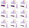 |
Fig. A.1. Corner plots of χ2 surface as a function of the model parameters (Δη, ζw) for MAGMA. The violet contours correspond to the minimum χ2 value. The top and right panels of each corner plot report the probability density distributions for the marginalized parameters; confidence intervals (±1σ) are shown as violet-tinted shaded rectangular regions, and the MLE (PDF mode for Δη, median for ζw) is shown by a vertical dashed line. Here, Δη ∈ [ − 10, 3.4] (see Fig. 1 for the “symmetric” Δη intervals). |
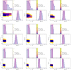 |
Fig. A.2. Corner plots of χ2 surface as a function of the model parameters (Δη, ζw) for MAGMA. The violet contours correspond to the minimum χ2 value. The top and right panels of each corner plot report the probability density distributions for the marginalized parameters; confidence intervals (±1σ) are shown as violet-tinted shaded rectangular regions, and the MLE (PDF median) is shown by a vertical dashed line. Here, Δη ∈ [0,3.4] (see Fig. 1 for the “symmetric” Δη intervals). |
Appendix B: SFHs and toy-model predictions for gas and stellar growth
In order to investigate the time derivatives of Mg and Mstar and their ratio, we introduce an arbitrary SFH. As a simple example, we have taken an exponential with arbitrary scaling defined by β and the star-formation time scale τSF:
 (B.1)
(B.1)
Equation (B.1) can be integrated to obtain Mstar [see Eq. (2)], at the current age of the galaxy tgal:
![Mathematical equation: $$ \begin{aligned} M_{\star }(t=t_{\rm gal}) = \frac{\psi _0\,\alpha \,\tau _{\rm SF}}{\beta }\,\left[\exp \left(\frac{\beta t_{\rm gal}}{\tau _{\rm SF}}\right) - 1\right]. \end{aligned} $$](/articles/aa/full_html/2022/01/aa40414-21/aa40414-21-eq49.gif) (B.2)
(B.2)
If we take the time-scale of star formation τSF to be equal to the gas depletion time τg [the inverse of ϵ⋆, see Eq. (13)], there are two unknowns in Eq. (B.2): tgal and ψ0 (β is fixed arbitrarily for rising and declining SFHs). However, ψ(tgal) = ψ0 exp(βtgal/τSF) = SFR and M⋆(tgal) = Mstar, are the observables that we measure, so that Eq. (B.2) can be solved for ψ0:
 (B.3)
(B.3)
This toy model also gives the initial gas mass Mi = ψ0τSF.
The remaining variable needed to define the galaxy’s evolutionary state is tgal, which can be established with ψ0 through Eq. (B.1):
 (B.4)
(B.4)
In case of a constant SFH (β = 0), with ψ(t) = ψ0 = SFR, the solutions are quite simple: M⋆(t) = Mstar, Mgas = Mi = SFR τSF, and Δη = α.
Figure B.1 shows the values inferred for tgal with the simple SFH of Eq. (B.1) with β = −1 (declining exponential) plotted against Mstar (top panel) and ψ0 plotted against Mstar (middle). Although there is significant scatter, galaxies with Mstar ≲ 109 M⊙ are apparently younger, with ages as low as 109 yr, rather than the overall inferred age of more massive galaxies, 1010 yr. The initial SFR ψ0 is very tightly linked with Mstar, over a dynamic range of ∼103. The bottom panel of Fig. B.1 illustrates that the total gas depletion times (i.e., including both molecular and atomic components) are relatively constant with Mstar.
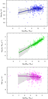 |
Fig. B.1. Inferred galaxy age tgal plotted against Mstar for MAGMA galaxies (top panel); initial SFR at t = 0, ψ0 plotted against Mstar (middle); τg (assumed equal to τSF) plotted against Mstar (bottom). In the two top panels, we assumed a simple declining exponential SFH with β = −1 [Eq. (B.1)], and that |
Now the only missing ingredient to describe Mg is Δη [see Eq. (14)]. Ultimately, the toy model presented here requires through Eq. (13) that the SFH given by Eq. (B.1) is related to the time evolution of Mg [Eq. (14)]. If  is the same as ϵ⋆, as we have assumed, the formalism requires:
 (B.5)
(B.5)
Thus, fixing β allows only certain values of Δη. Figure B.2 shows the time evolution of Mg and Mstar over the last 50% of the galaxies’ lifetime, assuming that tgal is given by Eq. (B.4), and ψ0 by Eq. (B.3). The different sets of curves correspond to different Mstar medians and the corresponding medians of τSF, tgal, and ψ0, while the vertical separation is achieved through the assignment of different Δη as required by β = ( − 1, 0, 0.1). The rising exponential SFH cannot have β arbitrarily large because otherwise Eq. (B.3) has negative values; β = 0.1 is close to the largest value allowed by the data. Figure B.2 clearly shows that according to the SFH, and the value of β and consequently Δη, dlog Mg/dlog Mstar can be positive or negative. Thus, it is difficult to assign Δη through the application of Eq. (27).
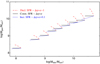 |
Fig. B.2. Time evolution of Mg vs Mstar over the last 50% of the galaxies’ lifetime, according to the toy-model based on three exponential SFHs: β = ( − 1, 0, 1), and also assuming that the SFR timescale τSF is the same as the gas depletion time, τg = |

Appendix C: The formalism for the “homogeneous wind”
In this paper we have determined solutions for Zg in the most general case of Zw ≠ Zg. We demonstrate (as already shown by Peeples & Shankar 2011) that in general this is a valid assumption since the outflowing gas Zw is not the same as the ISM gas, Zg, especially at low masses (e.g., Chisholm et al. 2015; Creasey et al. 2015; Muratov et al. 2017).
However, much earlier work assumed, instead, that Zw = Zg, adopting the so-called homogeneous wind model (e.g., Pagel 2009; Erb 2008). This assumption leads to ζw = ηw, and modifies Eq. (15) as follows:
![Mathematical equation: $$ \begin{aligned} Z_g = \left(\frac{q}{\eta _a}\right)\, \left[1 - \left(\frac{M_g}{M_i}\right)^{\frac{\eta _a}{\alpha - \eta _a + \eta _w}}\right]. \end{aligned} $$](/articles/aa/full_html/2022/01/aa40414-21/aa40414-21-eq56.gif) (C.1)
(C.1)
This solution, already reported by Erb (2008) in her Eq. 11, places the dependence of ηw only in the exponent of Mg/Mi, while ηa also appears in the denominator in the Zg expression.
The very interesting outcome of this exercise is that the ηw derived in this way reproduce the values of ζw shown in Fig. 3 and obtained using the more general formalism (using Zw ≠ Zg) of Eq. (15). Thus, metal loading ζw and mass loading ηw in the winds can be confused, depending on the assumptions made in the application of the formalism.
All Tables
All Figures
|
Fig. 1. Corner plots of χ2 surface as a function of the model parameters (Δη, ζw) for MAGMA binned by Mstar. The violet contours correspond to the minimum χ2 value. The top and right panels of each corner plot report the probability density distributions for the marginalized parameters; confidence intervals (±1σ) are shown as violet-tinted shaded rectangular regions, and the MLE (PDF median) is shown by a vertical dashed line. |
| In the text | |
|
Fig. 2. Difference of mass-loading factors Δη (top panel) and metal-loading factors ζw (bottom panel) as a function of virial velocities obtained from the BTFR from Sales et al. (2017). In both panels, filled symbols show the Bayesian results, and in the top panel, open ones illustrate the upper bound of the PDF 1σ confidence intervals (CI). Different symbol types correspond to the interval of Δη in the Bayesian priors, as described in the text; the symbols for Δη ∈ [0, 3.4] and Δη ∈ [ − 10, 3.4] are (arbitrarily) offset along the abscissa for better visibility. The gray regions give the ±1σ uncertainties in the best-fit values. Also shown is the “equilibrium” asymptote, namely Δη = α (see Sect. 3.1). In the top panel, the two estimates of Δη from different priors are exactly coincident. In the bottom panel, the formulations by Peeples & Shankar (2011) for two O/H calibrations, redone here for our value of y, are given by (purple) short-dashed and (blue) long-dashed curves for the PP04N2 and D02 calibrations, respectively. Also shown are the metal-loading factors computed by Chisholm et al. (2018) from COS data. The text gives more details. |
| In the text | |
|
Fig. 3. Difference of mass-loading factors Δη and metal-loading factors ζw inferred from the Bayesian analysis, and observed Zg in the bottom panel, as a function of Mstar on the left, and as a function of μg on the right. In the two upper panels, the best-fit Bayesian values are shown as filled symbols (circles or squares according to the Δη prior), with error bars corresponding to the ±1σ excursion, which is also illustrated by light-gray shaded regions. The rightmost point (magenta circle) in the top and middle right panels corresponds to the “extra” high-μg bin shown in Fig. 6. In the top panels, a horizontal dashed line illustrates the “equilibrium solution” with Δη = α. In the top left panel, the (purple) dashed curve is a linear power-law fit of Δη to log(Mstar), while the dashed curve in the top right panel shows Eq. (27), with d log Mg/d log Mstar = 0.72, as found in Paper II. The fits to the curves for ζw in the middle panels are cubic: log(ζw) as a function of log(Mstar) in the left panel, and ζw as a function of Fg in the right. In the lower panels, observed MAGMA Zg are shown as small filled circles, color coded by gas fraction, while the Zg medians and 1σ deviations are shown by large (black) filled circles and error bars. The dashed curves in the lower panels correspond to the calculation of Zg based on the fits in the upper panels (as a function of μg on the left, and log(Mstar) on the right): the long-dashed curves (dark orange) correspond to the Δη ≥ 0 priors, while the short-dashed ones (purple) to the “symmetric” priors. The green curves in the left panels are described in the text, obtained by fitting individual galaxy Δη and ζw calculated using Eqs. (27) and (28). |
| In the text | |
|
Fig. 4. Baryonic gas fraction μg plotted against (log) Mstar for MAGMA galaxies. Galaxies are coded by gas fraction, Fg, as shown in the vertical color bar. MAGMA medians are shown as a heavy gray line, with ±1σ excursions as the gray region. As noted in the text, the two low-mass galaxies with low μg are Sextans A and WLM, with probable substantial underestimates of the total gas content. |
| In the text | |
|
Fig. 5. Corner plots of χ2 surface as a function of the model parameters (Δη, ζw) for MAGMA binned by μg. The violet contours correspond to the minimum χ2 value. The top and right panels of each corner plot report the probability density distributions for the marginalized parameters; confidence intervals (±1σ) are shown as violet-tinted shaded rectangular regions, and the MLE (PDF mode for Δη, median for ζw) is shown by a vertical dashed line. |
| In the text | |
|
Fig. 6. Corner plot of χ2 surface as a function of the model parameters (Δη, ζw) for the highest μg bin MAGMA, here with a higher boundary than in Fig. 5: μg > 0.75. As in previous figures, the violet contours correspond to the minimum χ2 value, and the top and right panels report the probability density distributions for the marginalized parameters. Confidence intervals (±1σ) are shown as violet-tinted shaded rectangular regions, and the MLE (PDF mode for Δη, median for ζw) is shown by a vertical dashed line. |
| In the text | |
|
Fig. 7. Effective yield as a function of μg. Galaxies are coded by gas fraction, Fg, as shown in the vertical color bar. MAGMA medians are shown as a heavy gray line, with ±1σ excursions as the surrounding gray regions. The two dashed curves correspond to the predictions from the Δη and ζw parameterizations (see also Fig. 3), with the symmetric Δη priors given as a short-dashed (purple) curve, and the Δη ≥ 0 priors as a long-dashed (orange) one. The horizontal dashed line corresponds to our adopted true yield y = 0.037 (see text). |
| In the text | |
|
Fig. 8. Effective yield as a function of Mstar (left panel) and Vcirc (right panel). Galaxies are coded by gas fraction, Fg, as shown in the vertical color bar. MAGMA medians are shown as a heavy gray line, with ±1σ excursions as the surrounding gray regions. Also shown in the left panel as two dashed curves are the predictions from the Δη and ζw parameterizations (see also Fig. 3), with the symmetric Δη priors given as a short-dashed (purple) curve, and the Δη ≥ 0 priors as a long-dashed (orange) one. The right panel illustrates galaxies with high star-formation efficiency (short gas depletion times) with a blue dashed curve, and those with low efficiency (long depletion times) as a red one. The horizontal short-dashed line corresponds to the yield of 0.037 adopted in this paper. See text for more details. |
| In the text | |
|
Fig. 9. Ratio of inferred wind and ISM metallicities Zw/Zg plotted against virial velocity Vcirc. Also shown (with arbitrary scaling) is the shape of Bayesian ζw as also plotted in Fig. 2; it is clearly not a power law, thus the different power-law forms of ηw introduce inflections in Zw/Zg. Left panel: as indicated in the legend, different trends of Zw/Zg are inferred by dividing the fitted form of ζw (see Eq. (22)) by various scalings of ηw (see text for more details). The shaded regions correspond to the trends allowed by the two different Bayesian estimates of ζw according to the different Δη priors. Right panel: broken-power law trend for ηw found by Muratov et al. (2015) is shown as a solid heavy (gray) curve, where the inflection at Vcirc = 60 km s−1 corresponds to a sharp decrease of Zw/Zg (see text for more details). The short-dashed (dark-blue) curve shows the relation found by Mitchell et al. (2020), in the low-mass regime where stellar feedback dominates, and the long-dashed (blue) curve shows the observed relation derived by Chisholm et al. (2018). |
| In the text | |
|
Fig. A.1. Corner plots of χ2 surface as a function of the model parameters (Δη, ζw) for MAGMA. The violet contours correspond to the minimum χ2 value. The top and right panels of each corner plot report the probability density distributions for the marginalized parameters; confidence intervals (±1σ) are shown as violet-tinted shaded rectangular regions, and the MLE (PDF mode for Δη, median for ζw) is shown by a vertical dashed line. Here, Δη ∈ [ − 10, 3.4] (see Fig. 1 for the “symmetric” Δη intervals). |
| In the text | |
|
Fig. A.2. Corner plots of χ2 surface as a function of the model parameters (Δη, ζw) for MAGMA. The violet contours correspond to the minimum χ2 value. The top and right panels of each corner plot report the probability density distributions for the marginalized parameters; confidence intervals (±1σ) are shown as violet-tinted shaded rectangular regions, and the MLE (PDF median) is shown by a vertical dashed line. Here, Δη ∈ [0,3.4] (see Fig. 1 for the “symmetric” Δη intervals). |
| In the text | |
|
Fig. B.1. Inferred galaxy age tgal plotted against Mstar for MAGMA galaxies (top panel); initial SFR at t = 0, ψ0 plotted against Mstar (middle); τg (assumed equal to τSF) plotted against Mstar (bottom). In the two top panels, we assumed a simple declining exponential SFH with β = −1 [Eq. (B.1)], and that |
| In the text | |
|
Fig. B.2. Time evolution of Mg vs Mstar over the last 50% of the galaxies’ lifetime, according to the toy-model based on three exponential SFHs: β = ( − 1, 0, 1), and also assuming that the SFR timescale τSF is the same as the gas depletion time, τg = |
| In the text | |
Current usage metrics show cumulative count of Article Views (full-text article views including HTML views, PDF and ePub downloads, according to the available data) and Abstracts Views on Vision4Press platform.
Data correspond to usage on the plateform after 2015. The current usage metrics is available 48-96 hours after online publication and is updated daily on week days.
Initial download of the metrics may take a while.