| Issue |
A&A
Volume 656, December 2021
|
|
|---|---|---|
| Article Number | A114 | |
| Number of page(s) | 17 | |
| Section | Planets and planetary systems | |
| DOI | https://doi.org/10.1051/0004-6361/202141824 | |
| Published online | 09 December 2021 | |
Evidence for stellar contamination in the transmission spectra of HAT-P-12b
1
CAS Key Laboratory of Planetary Sciences, Purple Mountain Observatory, Chinese Academy of Sciences, Nanjing 210023, PR China
2
School of Astronomy and Space Science, University of Science and Technology of China, Hefei 230026, PR China
e-mail: This email address is being protected from spambots. You need JavaScript enabled to view it.
, This email address is being protected from spambots. You need JavaScript enabled to view it.
3
CAS Center for Excellence in Comparative Planetology, Hefei 230026, PR China
4
Instituto de Astrofísica de Canarias, Vía Láctea s/n, 38205 La Laguna, Tenerife, Spain
5
Departamento de Astrofísica, Universidad de La Laguna, 38206 La Laguna, Spain
6
Institut für Astrophysik, Georg-August-Universität, Friedrich-Hund-Platz 1, 37077 Göttingen, Germany
Received:
19
July
2021
Accepted:
22
September
2021
Abstract
Context. Transmission spectroscopy characterizes the wavelength dependence of transit depth, revealing atmospheric absorption features in planetary terminator regions. In this context, different optical transmission spectra of HAT-P-12b reported in previous studies exhibited discrepant atmospheric features (e.g., Rayleigh scattering and alkali absorption).
Aims. We aim to understand the atmosphere of HAT-P-12b using two transit spectroscopic observations by the Gran Telescopio Canarias (GTC) and to search for evidence of stellar activity contaminating the transmission spectra, which might be the reason behind the discrepancies.
Methods. We used Gaussian processes to account for systematic noise in the transit light curves and used nested sampling for Bayesian inferences. We performed joint atmospheric retrievals using the two transmission spectra obtained by GTC OSIRIS, as well as previously published results, coupled with stellar contamination corrections for different observations.
Results. The retrieved atmospheric model exhibits no alkali absorption signatures, but shows tentative molecular absorption features including H2O, CH4, and NH3. The joint retrieval of the combined additional public data analysis retrieves similar results, but with a higher metallicity.
Conclusions. Based on Bayesian model comparison, the discrepancies of the transmission spectra of HAT-P-12b can be explained by the effect of different levels of unocculted stellar spots and faculae. In addition, we did not find strong evidence for a cloudy or hazy atmosphere from the joint analysis, which is inconsistent with prior studies based on the observations of the Hubble Space Telescope.
Key words: planets and satellites: atmospheres / planets and satellites: individual: HAT-P-12b / techniques: spectroscopic
© ESO 2021
1 Introduction
According to the NASA Exoplanet Archive1 (as of July 2021), more than 4400 exoplanets have been discovered, among which only ~100 have been observed using transmission spectroscopy. A transmission spectrum presents the wavelength dependency of planetary transit depth and may indicate the atmospheric absorption and scattering features at the planetary terminator (Seager & Sasselov 2000; Brown 2001). By computing the radiative transfer of the stellar light passing through the planetary atmosphere, we can retrieve a one-dimensional atmospheric model that constrains its physical properties and chemical compositions, including the atmospheric temperature, metallicity, carbon-to-oxygen ratio, abundances of atomic and molecular species, and the presence of clouds or hazes (Madhusudhan & Seager 2009).
The exoplanet HAT-P-12b is an interesting target and there are many related studies on its transmission spectroscopy (e.g., Line et al. 2013; Mallonn et al. 2015; Sing et al. 2016; Barstow et al. 2017; Tsiaras et al. 2018; Alexoudi et al. 2018; Fisher & Heng 2018; Pinhas et al. 2019; Deibert et al. 2019; Wong et al. 2020; Yan et al. 2020). According to Hartman et al. (2009) and Mancini et al. (2018), it is a low-density warm sub-Saturn with a mass of 0.201 ± 0.012 MJ, a radius of 0.919 ± 0.023 RJ, and an equilibrium temperature of 955 ± 11 K. It orbits a K4 dwarf with a period of ~3.21 days at a distance of ~0.038 AU. The host star HAT-P-12 has a mass of 0.691 ± 0.023 M⊙, a radius of 0.679 ± 0.013 R⊙, and an effective temperature of 4665 ± 50 K. Line et al. (2013) measured the near-infrared (NIR) transmission spectrum of HAT-P-12b using the Hubble Space Telescope Wide Field Camera 3 (HST WFC3), which was observed before the implementation of the spatial scan mode (Deming et al. 2013). They failed to detect the expected water absorption. Sing et al. (2016) combined optical spectroscopy from the Space Telescope Imaging Spectrograph (HST STIS), NIR spectroscopy from HST WFC3, and broad-band photometry at 3.6 and 4.5 μm from the Infrared Array Camera (IRAC) of the Spitzer Space Telescope. Their results show a Rayleigh scattering slope caused by haze aerosols and a possible potassium absorption signal. Wong et al. (2020) reanalyzed the data used in Sing et al. (2016) coupled with two more transits observed in the spatial scan mode of the HST WFC3 and two secondary eclipses using broad-band photometry from Spitzer IRAC. They found a cloudy and hazy atmosphere without alkali features. In contrast to the space-based observations, the ground-based observations reported by Mallonn et al. (2015) and Yan et al. (2020) presented relatively flat and featureless transmission spectra in the optical, favoring a cloudy atmosphere. Alexoudi et al. (2018, 2020) propose that such a discrepancy in the offsets and slopes of transmission spectra can be attributed to the inaccuracy of orbital geometry parameters (semi-major axis, orbitalinclination, or impact parameters) used in the spectroscopic light curve fitting. In addition, Deibert et al. (2019) performed high-resolution transit spectroscopy on HAT-P-12b, and they revealed a 3.2σ detection of sodium absorption for the first time.
In this study, we analyze the optical transmission spectra of HAT-P-12b observed by the Optical System for Imaging and low-Intermediate-Resolution Integrated Spectroscopy (OSIRIS; Cepa et al. 2000) at the Gran Telescopio Canarias (GTC). We aim to validate the absorption signals of sodium and potassium and the Rayleigh scattering slope in the optical band and to compare our results with previous observations using other instruments.
In the next section, we summarize the observation details and data reduction processes. Then we introduce our method of transit light curve analysis and present the transmission spectra in Sect. 3. The atmospheric retrieval is illustrated in Sect. 4. We discuss other possible interpretations of the transmission spectra in Sect. 5 in comparison with prior studies. We draw our conclusions in Sect. 6.
2 Observations and data reduction
2.1 Transit spectroscopy observations
Two transit events of HAT-P-12b were observed by GTC OSIRIS in the long-slit spectroscopy mode on the nights of 20 Apr. 2012 (hereafter OB12) and 17 Mar. 2013 (hereafter OB13), respectively. During the observations, one reference star GSC2 N130301284 was simultaneously observed for differential spectrophotometry. The target and the reference stars have comparable r-magnitudes, which are 12.33 and 12.84 (Zacharias et al. 2015), respectively. They were aligned through a 12″-wide and 7.4′ -long slit perpendicular to the dispersion direction with a distance of 2.44′. The pixel scale was 0.254″ after a 2 × 2 pixel binning. The detector of OSIRIS consists of a mosaic of two Marconi CCDs (1024 × 2048 pixels after 2 × 2 pixel binning) with a 9.4″ gap between them. In OB12, the target star was placed on CCD1 and the reference star was on CCD2, while in OB13, both stars were placed on CCD2. An R1000R grism was used to acquire the stellar spectra with a dispersion of 2.62 Å per pixel, covering a wavelength range of 5100–10 000 Å. More observation details are listed in Table 1.
We note that the dome shutter of GTC could not be fully opened before November 20152. Therefore partial dome vignetting was likely presented for frames acquired with elevations above ~72 degrees3. This problem can introduce significant but smooth systematics in the OB12 light curves, as it occurred from the eighth to the 114th frames. However, this problem is negligible for the OB13 dataset because the corresponding elevations were lower than 72 degrees during the observation.
In addition, a subset of the OB12 spectral images was contaminated by a moving ghost that could originate from an instrumental internal light reflection. This ghost showed up in a total of 83 frames during OB12 and overlapped with a few pixels of the target’s spectrum for 30 frames. The intensity of the ghost was two orders of magnitude smaller than the peak values of stellar flux. For white-light curves, it has negligible influence after a broadband integration. But for spectroscopic light curves,it would cause significant flux anomalies when the ghost overlapped with the target’s spectrum. Figure A.1 presents its shape and trace on CCD1, along with the resulting flux anomalies in the spectroscopic light curves.A similar case is reported by Nortmann et al. (2016) in their GTC spectroscopic observations of HAT-P-32b.
Details of two transit observations for HAT-P-12b.
2.2 Data reduction
We reduce the spectral data following the procedures described in Chen et al. (2017). The frames of OB12 and OB13 were calibrated separately, but using the same procedures of the IRAF programs (Tody 1993), including corrections for overscan, bias, flat fields, cosmic rays, and sky background. The wavelength calibration was done utilizing the arc lines of HgAr, Xe, and Ne observed through a narrower slit with the same R1000R grism. The best aperture size for extracting spectra was evaluated by minimizing the scatter of white-light curves, and diameters of 25 pixels (6.35″) and 37 pixels (9.40″) were chosen for OB12 and OB13, respectively. Figure 1 shows the stacked stellar spectra extracted using the best aperture sizes. We adopted an overall 20-nm wavelength binning in the range from 519.3 to 759.3 nm and from 766.2 to 918.2 nm. Narrower 4-nm bins were adopted centered around the sodium D-lines (~589.3 nm) and the potassium D-lines (~768.2 nm). The light curve in the range of 759.3–766.2 nm had a large scatter and a lower signal-to-noise ratio (S/N) due to the strong absorption of the telluric oxygen A-band (759–770 nm), which is likely to impact the planetary transmission signal at the potassium D2-line (~766.5 nm), while the telluric oxygen B-band (~689 nm) and water absorption (~820 nm) have negligible impacts after differential spectrophotometry. Therefore we excluded the narrow oxygen A-band in the light curve analyses. In addition, we also excluded the spectra with wavelength larger than 918.2 nm because of their low fluxes and strong fringing modulation at the red end.
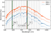 |
Fig. 1 Stellar spectra of the target star HAT-P-12 (darker) and reference star GSC2 N130301284 (lighter) in OB12 (orange) and OB13 (blue). The dashed lines are passbands for spectroscopic light curves. The green solidlines indicate the D-lines of Na and K. The red-shaded band is strongly affected by the telluric O2 absorption. The stellar fluxes have been normalized and arbitrarily shifted for clarity. |
3 Transit light curve analysis
3.1 White-light curves
The transit model is computed using batman (Kreidberg 2015) following the analytic model of Mandel & Agol (2002). The free parameters of the transit model include radius ratio Rp ∕Rs, quadratic limb-darkening coefficients (LDCs) u1 and u2, orbital semi-major axis relative to stellar radius a∕Rs, orbital inclination i, and central transit time tc. According to Hartman et al. (2009), we adopt a circular orbit and use their transit ephemeris to estimate the priors of tc :
 (1)
(1)
where n is the orbit number (n = 504 for OB12; n = 607 for OB13).
We apply Gaussian process (GP) regression to predict the systematic noise of transit light curves. This method has been introduced in Gibson et al. (2012) and is further applied in Pont et al. (2013), Evans et al. (2016) and Sedaghati et al. (2017), etc. We use celerite developed by Foreman-Mackey et al. (2017) to implement fast one-dimensional GP regression. In our GP modeling, the normalized flux curve f(t) is fitted by the sum of a mean model μ(t;θ) and a predictive curve g(t;φ) sampled from the GP model:
 (2)
(2)
where ε is white noise, t is the time vector, θ and φ are the free parameters of the mean model and the kernel function, respectively. The mean function μ(t) for white-light curves is just the transit model m(t):
 (3)
(3)
where θ = (Rp∕Rs, u1, u2, a∕Rs, i, tc). The predictive curve g(t) is sampled with a covariance matrix K determined by a GP kernel function k(τ). Rasmussen & Williams (2006) provides a detailed introduction to various GP kernels. Normally, a squared exponential (SE) kernel or a Matérn class kernel are flexible enough to account for the correlated noise. The former is infinitely differentiable and thus generates very smooth predictive curves, while the latter has variable levels of smoothness depending on its hyper-parameter ν (see Eq. (4.14) in Rasmussen & Williams 2006). For large values of ν, for example ν ≥ 7∕2, the corresponding GPs are indistinguishable from those generated by an SE kernel. In the ground-based transit observations, the systematic noise may have rough changes due to seeing variation or pointing jitters. Therefore we select the 3∕2-order Matérn kernel (ν = 3∕2) to fit the light-curve systematics, which has the form
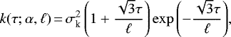 (4)
(4)
where τ = |ti − tj| is the distance in time between two data points,  and ℓ are the variance and the length scale of systematic noise. The estimated flux errors are added to the diagonal of the covariance matrix. So the elements of the covariance matrix are
 (5)
(5)
where φ = (σadd, σk, ℓ), and δij is the Kronecker delta function. The error σph is the photon-dominated noise previously determined from reduced images, which underestimates the true white noise. Therefore, we use a free parameter σadd to account for additional jitters.
We utilize the nested sampling algorithm (Skilling 2004; Feroz & Hobson 2008) to estimate model evidence and parameter distributions in a Bayesian framework. The package PyMultiNest (Buchner et al. 2014) is used, which is a Python implementation of the code MULTINEST (Feroz et al. 2009). In our light curve analyses, we calculate the parameter posteriors using 1000 live points and a sampling efficiency of 0.3 in PyMultiNest. The nested sampling is terminated when the contributions of the remaining prior space to  is less than 0.1. The posterior distributions are determined with ~10 000 accepted samples from a total of ~600 000 samples. The parameter estimates are consistent in multiple runs.
We adopt uniform priors on the radius ratio Rp∕Rs, the relative semi-major axis a∕Rs, the orbital inclination i, and the central transit time tc. We find it difficult to constrain the quadratic LDCs with the observed light curves. Therefore, we assume Gaussian priors for u1 and u2 based on the ATLAS model calculated by the code of Espinoza & Jordán (2015) using the stellar parameters of HAT-P-12. The GP parameters σadd, σk, and ℓ are constrained by log-uniform priors.
We use asingle set of transit parameters (except tc) to fit the white-light transit model of OB12 and OB13 but different GPs to fit the different systematics. The global log-likelihood function is the sum of the log-likelihood for each GP. To demonstrate the consistency in the transit parameters between the two observations, we also perform individual analysis for each white-light curve. The white-light parameters derived from joint and individual analyses are listed in Table 2. The best-fit light curves and the extracted systematics are shown in Fig. 2. The results are consistent between OB12 and OB13 and also consistent with prior literature values of Wong et al. (2020).
3.2 Spectroscopic light curves
We separately fit each spectroscopic light curve and estimate the wavelength-dependent transit parameters Rp ∕Rs, u1, and u2. The wavelength-independent parameters (a∕Rs, i, tc) are fixed to the median estimates derived from the joint analysis of white-light curves (Table 2). In addition, a baseline is added to the mean function to account for the common-mode systematics. In some studies, for instance Kreidberg et al. (2014) and Gibson et al. (2017), the spectroscopic light curves are divided by the best-fit white-light systematics model to reduce the amplitudes of systematics and also avoid introducing additional parameters. As discussed in Gibson et al. (2017), such a “divide-white” method is based on the assumption that the systematics are mainly wavelength-independent. However, with regard to OB12 and OB13, the spectroscopic systematics exhibits wavelength dependence to some extent (Figs. A.2 and A.3). In this case, the “divide-white” method would instead introduce additional noise in those passbands with weaker systematics. Therefore, we allow the common mode w(t) to have a variable amplitude α(λ), making it adaptive to the specific systematics in each passband. So the mean function for spectroscopic light curves becomes
 (6)
(6)
where  . The common modes w = fwhite − mwhite are determined from the best-fit white-light curves for OB12 and OB13 separately. We assume a uniform prior of
  for α. The amplitude α is larger than one when the spectroscopic systematics have larger amplitudes than w(t) and is close to zero when the common mode feature is quite weak.
As mentioned in Sect. 2.1, the observed spectra in OB12 were occasionally covered by a moving ghost (Fig. A.1). The affected range is 520–552 nm and 750–825 nm in wavelength. It is difficult to fit these flux anomalies using a GP or a parametric baseline function, for which we have to treat these points as outliers. We inspected all 30 frames where the ghost overlapped with the stellar spectrum and discarded them in our spectroscopic light curve analysis.
Figures A.2 and A.3 show the fitting results of spectroscopic light curves of OB12 and OB13, respectively. It is evident that the spectroscopic systematics have smaller amplitudes at the blue and red ends. We compared the Bayesian evidence between the “divide-white” method and the “variable-common-mode” method when fitting the spectroscopic light curves and found stronger evidence for the latter in most wavebands (Fig. A.4). We calculated the Pearson correlation coefficients of the common-mode amplitudes α and the flux response in narrow passbands, which are 0.91 for OB12 and 0.85 for OB13, indicating that α is actually strongly correlated with flux for both observations (Fig. A.5). Therefore, we consider that in the cases of OB12 and OB13, the “variable-common-mode” method has a better performance than the “divide-white” method in reducing the spectroscopic systematics.
We present the transmission spectra of HAT-P-12b in Fig. 3 and list the posterior estimates of Rp ∕Rs in Table 3. The transmission spectrum of OB12 is slightly different from that of OB13 and shows a larger slope in the range of 550–800 nm. In Sect. 2.1, we mentioned that the OB12 observation was affected by dome vignetting and an instrumental internal light reflection. The effect of dome vignetting could introduce significant but smooth systematics to the light curves of both stars in OB12, which has been removed by GP regression and should not cause wavelength-dependent biases. Regarding the “moving ghost”, only a small part of data points were affected and we have removed them as outliers (Fig. A.1), which should not be responsible for biases ina large wavelength range. Alexoudi et al. (2018, 2020) suggest that a fixed but inaccurate orbital inclination or impact parameter will cause a different slope and a systematic offset in the optical transmission spectrum. As illustrated in Fig. 4, although there is a strong correlation in the joint distributions of a∕Rs and i, our derived parameters are well consistent with other literature estimates. Furthermore, we applied the same values of a∕Rs and i derived from the joint analysis of white-light curves to all spectroscopic light curves of both observations. Thus the discrepancy between these two transmission spectra should not be attributed to the potential biases of orbital parameters. Instead we attribute such systematic bias to different levels of stellar activity during OB12 and OB13, and interpret these two sets of results using the same planetary atmospheric model but the separate parameters accounting for stellar contamination.
Transit parameters from broadband light curve fitting.
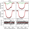 |
Fig. 2 Joint white-light curve fitting of OB12 (left column) and OB13 (right column). Top panels: observed white-light curves (black dots), along with the best-fit curves (red lines) and systematics (green lines). Mid panels: detrended white-light curves (black dots) and the best-fit transit models (red lines). Bottom panels: residuals of light-curve fitting. |
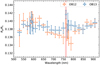 |
Fig. 3 Transmission spectra of OB12 (orange) and OB13 (blue). The red-shaded passband indicates the telluric O2 A-band. |
Radius ratios estimated from the spectroscopic light curves.
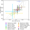 |
Fig. 4 Posterior estimates of the orbital geometry parameters of HAT-P-12b compared with other literature values. The error bars indicate 1σ credible intervals. The contours indicate 1–3σ joint credible regions from nested sampling. |
4 Atmospheric retrieval
4.1 Forward atmospheric modeling
We analyze the transmission signals of HAT-P-12b using a one-dimensional isothermal model atmosphere calculated by PLATON (Zhang & Chachan 2019; Zhang et al. 2020). In this model, the chromatic transit depths are mainly contributed to by gas absorption, collisional absorption, Mie scattering, and the effect of unocculted stellar spots and faculae. The atmospheric pressure is limited in the range of 108 –10−4 Pa and is equally divided into 500 layers in the logarithmic scale. The planetary radius at a reference pressure of 105 Pa is a free parameter to determine the height of each atmosphere layer. The chemical abundances for calculating the absorption coefficients of each layer are based on the equilibrium chemistry model with 34 atomic and molecular species computed by GGChem (Woitke et al. 2018), which are: H, He, C, N, O, Na, K, H2, H2O, CH4, CO, CO2, NH3, N2, O2, O3, NO, NO2, C2H2, C2H4, H2CO, H2S, HCl, HCN, HF, MgH, OCS, OH, PH3, SiH, SiO, SO2, TiO, and V O. The sources of spectral line lists include ExoMol (Tennyson & Yurchenko 2018), HITRAN 2016 (Gordon et al. 2017), CDSD-4000 (Tashkun & Perevalov 2011; Rey et al. 2017), and NIST (Sansonetti & Martin 2005). The collisional absorption coefficients are from HITRAN (Richard et al. 2012). The main parameters to control the chemical abundances are atmospheric temperature (T), metallicity (Z), and carbon-to-oxygen ratio (C/O). The forward modeling of transmission spectra is based on the opacity line lists with a resolution of λ∕Δλ = 10 000 as suggested by Zhang & Chachan (2019). The high-resolution opacities are then integrated to the same wavelength bins as those in Table 3 such that the likelihood function can be calculated.
The modeling of atmospheric condensates considers Mie scattering. We assume an optically thick cloud deck uniformly covering the planet and vertically extending to a pressure Pcld, below which the atmosphere is completely occulted by the opaque cloud while above atmospheric aerosols account for Mie scattering. As presented in the study of GJ 3470b by Benneke et al. (2019), Mie scattering can be used to characterize scattering-induced opacities for all wavelengths, and it asymptotically approaches Rayleigh scattering for particle sizes much smaller than the wavelength. The package PLATON uses the same algorithm as LX-MIE (Kitzmann & Heng 2018) to calculate the cross-sections of aerosol particles and allows the computation of Mie scattering for three condensates (MgSiO3, SiO2, and TiO2) using their actual wavelength-dependent refractive indices from Kitzmann & Heng (2018). We adopt MgSiO3, whose condensation temperaturevaries from ~1000 K at 1 Pa to ~1700 K at 105 Pa, as the major condensate for the atmosphere of HAT-P-12b, although the results are statistically undistinguishable if the other two species were selected. The aerosol particle size is assumed to have a mean size rm and a standard deviation of 0.5 in a log-normal distribution. The vertical variation of aerosol number density is determined by the function n0 ⋅ exp(−h∕Haero), where n0 is the maximum number density, h is the height above the cloud top, and Haero is the aerosol scale height. Therefore, the free parameters for Mie scattering are the cloud-top pressure Pcld, the aerosol scale height relative to gas scale height Haero∕Hgas, the mean radius rm, and the maximum number density n0 of aerosol particles.
4.2 Stellar contamination correction
The photometric monitoring of HAT-P-12’s activity presented by Wong et al. (2020) covers the transit epochs of OB12 and OB13. The differential magnitudes in the Cousins R band are − 0.2689 ± 0.0046 and − 0.2708 ± 0.0042 in the two observation seasons (Sep. 2011 – Jun. 2012; Sep. 2012 – Jun. 2013), but we cannot rule out the possibility of stellar activity with R-band variation amplitudes less than the uncertainties. Johnson et al. (2021) perform forward modeling on rotational variability in the Kepler and TESS bands. They find that the range of variability for K0 dwarfs can be less than 0.6% when assuming a spot area coverage of 20% and a temperature contrast of 560 K between the spots and the photosphere, and that the presence of faculae has relatively little influence on the variability. Meanwhile, the light curve of OB13 exhibits dip-like features near the central transit, which might be a hint of faculae occulted by the planet. Therefore, we attempt to explain the discrepancy in transit depths between OB12 and OB13 with stellar contamination composed of spots and faculae.
When a planet is transiting its host star, the presence of unocculted spots and faculae may cause significant wavelength-dependent offset of transit depth over a large wavelength range (McCullough et al. 2014; Rackham et al. 2018, 2019). This can be accounted by the change of stellar spectrum due to the temperature contrast between the active and the quiescent areas on the photosphere. The observed transmission spectrum will present positive offsets in the spot-dominated circumstances but negative offsets in the facula-dominated circumstances. In addition, these offsets are more significant at bluer wavelengths than at redder ends. Following Zhang & Chachan (2019), we correct this effect by

where  is the transit depth calculated from the forward atmospheric model without considering stellar contamination, βλ is the correction factor at wavelength λ, Sλ (T) is the stellar spectra interpolated in the BT-NextGen (AGSS2009) stellar spectral grid (Allard et al. 2012), Tphot, Tspot, and Tfacu are the temperatures of the quiescent photosphere, spots, and faculae, respectively, ϕspot and ϕfacu are the coverage fractions of spots and faculae. Other contributions such as the limb-darkening of spots and faculae or the magnetic-dependent effects are not considered in this correction.
We adopt the effective temperature of HAT-P-12 measured by Mancini et al. (2018) as an approximation of the photospheric temperature and thus Tphot = 4665 K. According to Fig. 7 in Berdyugina (2005), the quiet-star-to-spot temperature contrast increases with stellar effective temperature from approximately 200 K in M4V to 2000 K in G0V. Considering that HAT-P-12 is a K4 dwarf, we assume a uniform prior for Tspot − Tphot of  . The temperature contrast between the faculae and the photosphere Tfacu − Tphot is assumed to follow
  . The coverage fractions ϕs and ϕf are allowed to vary independently in a uniformprior of
  . The data of OB12 and OB13 are fitted by the same atmospheric model but corrected by separate stellar contamination parameters (Tspot, Tfacu, ϕspot, ϕfacu). Thus, a total of eight free parameters are added to the retrieval algorithm.
4.3 Retrieval results
The atmospheric retrieval is conducted with the nested sampling algorithm. We assume uniform or log-uniform priors for all free parameters. The total log-likelihood is the sum of the log-likelihood function for each observation. We set 1000 live points and a sampling efficiency of 0.3 in PyMultiNest, and acquired ~22000 accepted samples among a total of ~1.3 million samples. The posterior estimates of all parameters are listed in Table 4. The corresponding joint distributions are shown in Fig. A.6. The isothermal atmospheric temperature of  K is much lower than the equilibrium temperature of 955 ± 11 K. Similar low values are retrieved by Tsiaras et al. (2018) (509 ± 174 K) and Pinhas et al. (2019) (
 K), whereas other literature estimates are closer to the equilibrium temperature, including the effective temperature of
  K from the LBT observation by Yan et al. (2020), and the dayside blackbody temperature of
  K from the secondary eclipse measurement of Spitzer IRAC by Wong et al. (2020). MacDonald et al. (2020) propose that a 1D retrieval model applied on an inhomogeneous terminator atmosphere can result in an underestimated atmospheric temperature. The atmospheric metallicity is estimated to be ~100.63 times the solar value, while the metallicity of HAT-P-12 measured by Mancini et al. (2018) is [Fe∕H] = −0.20 ± 0.09. Therefore our estimated atmospheric metallicity is approximately ten times that of the host star. Considering the low mass of HAT-P-12b (Mp ~ 0.2 MJ), this agrees with the mass-metallicity relation presented by Thorngren et al. (2016), who suggest that lower mass planets have weaker ability to accrete hydrogen and helium during their formation hence resulting in higher metallicity. The opaque cloud deck is found to exist at lower altitudes than the previous literature estimates, and the cloud-top pressure is higher than ~0.6 bar in a 95% credible interval. The other parameters for Mie scattering (rm, Haero∕Hgas, n0) have large uncertainties in line with the absence of scattering features.
Figure 5 illustrates the model transmission spectrum derived from the joint retrieval after the stellar contamination correction. According to our stellar contamination model, the transmission spectrum of OB12 exhibits a lower spot-to-photosphere temperaturecontrast but a higher spot coverage fraction compared with those of OB13, which is due to the degeneracy between Tspot and ϕspot (Fig. A.6), whereas the retrieved facula temperatures and coverage fractions are consistent between the two observations. The facula-to-spot area ratio (Q = ϕfacu∕ϕspot) are estimated to be  for OB12 and
  for OB13. According to Chapman et al. (1997), the solar Q value is found to be 16.7 ± 0.5 for a 7.5 yr period during solar cycle 22 and increased as the solar cycle progressed. Herrero et al. (2016) suggest that this ratio tends to be smaller for more active K and early-M dwarfs. Therefore, our results suggest that stellar activity during OB12 was slightly stronger than during OB13. However, the stellar activity index
  of HAT-P-12b is measured tobe − 4.9 ± 0.1 by Mancini et al. (2018) using the HARPS-N spectra, which indicates low activity. We note that the spectra of HAT-P-12b in Mancini et al. (2018) were observed in March and April 2015, more than two years after the OSIRIS observations. Thus it is possible that the level of stellar activity varied during this time.
The major species that contribute to gas absorption features are found to be H2O, CH4, and NH3 (Fig. 6) because of the high carbon-to-oxygen ratio of 1.5 ± 0.3, whose corresponding volume mixing ratios (in log10) are  ,
,  , and
, and  . Although other common species may also have considerable mixing ratios under the assumption of equilibrium chemistry, they have negligible absorption features in the optical thus are not presented in Fig. 6, including CO (
 ), CO2 (
 ), N2 (
 ), H2S (
 ), etc. The retrieved water abundance is consistent with prior literature values (− 3.61 ± 1.48, Tsiaras et al. 2018;
  , Pinhas et al. 2019). In addition, the chemistry model attributes the absorption peak at ~590 nm to the minor absorption from water rather than sodium. The alkali-metal atoms, including Na and K, are found to be depleted in this atmosphere according to the equilibrium chemistry model, whose abundances are approximately 3 × 10⁻¹² (Na) and 1 × 10⁻¹³ (K). We note that Deibert et al. (2019) report a possible detection (3.2σ) of sodium absorption with high resolution transit spectroscopy, which would indicate certain mechanisms to keep the sodium atoms aloft in the upper atmosphere. The high abundance of methane is never reported in prior studies, but it is favored by the OSIRIS data to account for the tentative absorption feature at ~890 nm.
Parameter estimates of the atmospheric retrieval.
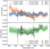 |
Fig. 5 Retrieved transmission spectra of HAT-P-12b. Upper panel: retrieved models composed of both model atmosphere and stellar contamination. Lower panel: transmission spectra and their retrieved models after stellar contamination correction. The model transmission spectra are wavelength-binned to a resolution of λ∕Δλ = 200. |
5 Discussion
5.1 Comparison with other atmospheric model assumptions
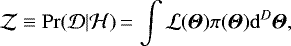
Here we examine other possible model assumptions and compare all these models based on their Bayesian evidence. Following the notation of Feroz et al. (2009), the model evidence (or marginal likelihood) in Bayes’ theorem is defined as
 (9)
(9)
where  is the data,
  is the model hypothesis,
  is the likelihood function, π is the prior function, Θ is the parameter vector, and D is its dimensionality. The evidence can be viewed as the average of the likelihood over the prior. With increasing dimensionality and broader prior space, the evidence will be exponentially weakened unless the maximum likelihood rises considerably, which embodies Occam’s razor. We conduct model comparison between two hypotheses
  and
and  by calculating the Bayes factor:
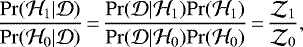 (10)
(10)
where the uninformative prior ratio 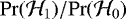 for the two hypotheses is set to unity. In practice, we calculate the log-evidence
  , and the logarithmic Bayes factor is simply
  . We interpret the Bayes factor based on the categories proposed by Kass & Raftery (1995). When
 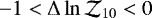 , there is weak evidence for
  against
  . When
 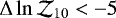 , there is very strong evidence for
  against
  .
.
When considering other potential model combinations, we mainly focus on the contributions from gas absorption, condensate scattering, and stellar contamination. Therefore a total of eight hypotheses can be proposed and evaluated. The simplest model is a pure atmosphere consisting of only hydrogen and helium ( ), where the H2 -H2 and H2-He collision-induced opacity and Rayleigh scattering are still considered, and it only has two free parameters: the reference planetary radius R0 and the atmospheric temperatureT. The most complicated model is the full model (
 ) proposed in Sect. 4.3, which has 16 free parameters, eight for the atmospheric model and the other eight for the stellar contamination correction. Since the estimated Bayesian evidence for
  could reach a precision of 0.12 when using 1000 live points and a sampling efficiency of 0.3 in PyMultiNest, we consider such hyperparameter settings are also suitable for other simpler model hypotheses. The actual computational cost largely depends on the specific model, from ~45 min for a null model
  up to ~64 h for a full model
  with 32-coreparallel computing (3.00 GHz CPUs).
Table 5 lists all eight hypotheses and their estimated model evidence. The model without condensate ( ) is calculated to have the largest model evidence. Comparing it with other models considering stellar contamination corrections (
 ,
,  , and
, and  ), there is quite weak evidence for condensate scattering, but very strong evidence for gas absorption. For those models excluding stellar contamination (
 ,
,  ,
,  , and
, and  ), their model evidences are considerably smaller than
  . Therefore, we can conclude that there is very strong evidence for the transmission spectra being affected by unocculted stellar spots and faculae but weak evidence for the presence of high-altitude clouds and hazes. This inference is different from other research papers on the atmosphere of HAT-P-12b. Though the stellar contamination model favored by Bayesian model comparison can explain a sufficient degree of variability in the data, it is not the only explanation for the change of transmission spectra. There are also other possible effects that might cause such variability or inconsistency (e.g., instrumental systematics or telluric effects).
Bayesian evidence under different atmospheric model assumptions.
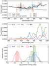 |
Fig. 6 Major chemical species contributing to gas absorption features. Top panel: solid line is the median model shown in the lower panel of Fig. 5. The dashed line is the same atmospheric model but assuming zero abundance of H2O, CH4, and NH3. The transmission spectra of OB12 and OB13 have been corrected for stellar contamination. Middle panel: contributions of gas absorption to the transmission spectra. Bottom panel: posterior distributions of the major species’ volume mixing ratios. |
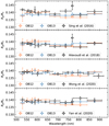 |
Fig. 7 Transmission spectra of OB12 and OB13 recalculated with similar wavelength bins used in other research papers. |
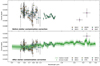 |
Fig. 8 Retrieval analysis joint with the transit depths presented in Yan et al. (2020) (LBT MODS) and Wong et al. (2020) (HST STIS G750; HST WFC3 G141; Spitzer IRAC). Upper panel: raw transmission spectra of the six data sets. Lower panel: shows the joint fit results with the effects of stellar contamination corrected for each data set. The green solid line is the median model with a resolution of λ∕Δλ = 200. The shaded areas indicate 68 and 95% credible intervals. The white dots are best-fit values calculated at the same wavelength bins as the corresponding data points. In the range of 0.5–1.0 μm, only the best-fit points corresponding to OSIRIS wavebands are displayed for clarity. |
5.2 Comparison with the published data
To examine the consistency among the optical transmission spectra observed by other instruments, we recalculate the transmission spectra of OB12 and OB13 using similar wavelength bins with those of Sing et al. (2016) (S16), Alexoudi et al. (2018) (A18), Wong et al. (2020) (W20), and Yan et al. (2020) (Y20), which are presented in Fig. 7. The optical spectra of S16, A18 and W20 were derived from the same data set of HST STIS, including the observations of two transits performed by STIS G430L grating and one transit performed by STIS G750L grating. The spectrum of Y20 was observed by the dual-channel mode of the multi-object double spectrograph (MODS) on the Large Binocular Telescope (LBT), and Fig. 7 shows the weighted means of MODS1 and MODS2. Our results are close to those of A18, W20, and Y20, while the values of S16 basically lie above our two sets of spectra. The discrepant results of S16 and A18 on the mean and slope of the spectra are mainly due to the discrepant values of orbital geometry parameters (see Fig. 4), but they both present a tentative detection of atomic potassium, which is however not detected or reported by other research including the high-resolution observation of Deibert et al. (2019).
Parameter estimates of atmospheric retrieval joint with other transmission spectra.
5.3 Joint retrieval with the published data
We can combine the OSIRIS transmission spectra with other transmission spectra to perform a joint retrieval considering stellar contamination, including the data from Yan et al. (2020) (LBT MODS) and Wong et al. (2020) (HST STIS G750L, HST WFC3 G141, and Spitzer IRAC). We note that Wong et al. (2020) perform a joint analysis of transit light curves based on two transits observed by HST WFC3 in the scan mode (12 Dec. 2015 and 31 Aug. 2016) and another two transits observed by Spitzer IRAC (3.6 μm on 8 Mar. 2013 and 4.5 μm on 11 Mar. 2013). The stellar contamination correction of Eq. (8) should not be applied on these multi-epoch NIR data sets. Fortunately, according to Fig. 3 of Pinhas et al. (2018), stellar contamination has weaker effects in NIR wavebands than in the optical and can be simply approximated as a transit depth offset or a rescaling factor. Furthermore, such a rescaling amplitude is within 1% for the IRAC wavebands, for which we can neglect the effect of stellar contamination on the IRAC data. Regarding the data from WFC3 G141, we replace βλ in Eq. (7) with a free parameter βWFC3 to apply independent rescaling of their transit depths. The transmission spectra of LBT MODS and HST STIS G750L were derived from single transit observations and contained sufficient data points (11 points for MODS and ten points for G750L), and thus we can apply the same correction method as we did for the OSIRIS data. In addition, although there are two observations by HST STIS G430L presented in Wong et al. (2020), they are excluded in our joint retrieval for two reasons. One is that only four data points are available for each observation of STIS G430L, which failed to constrain the atmospheric model after a four-parameter stellar contamination correction (ΔTspot, ΔTfacu, ϕspot, and ϕfacu). The other reason is that the rescaling approximation applied to the NIR bands of WFC3 G141 is unsuitable for the NUV-to-optical bands of STIS G430L where the stellar contamination effect is highly wavelength dependent, as it has been shown in Fig. 5, as well as Fig. 3 of Pinhas et al. (2018).
Figure 8 shows the results of this joint retrieval, where the posterior estimates of corresponding model parameters are listed in Table 6. To reduce the computational cost, we adopted the pre-computed line lists with a lower resolution of λ∕Δλ = 1000 in this part. The model inference is basically consistent with our previous analysis using the OSIRIS data alone. There are evident gas absorption features in the optical and NIR wavebands. Although the signatures of methane are disfavored by the IRAC data, the atmospheric model still exhibits a low temperature of  K and a high C/O ratio of
  . The metallicity is found to be ~100 times solar, which is higher than our previous estimate but consistent with that of Wong et al. (2020). The model of condensate scattering is still poorly constrained, indicating low evidence for high-altitude clouds and hazes. We also show that the discrepancy between different transmission spectra can be reduced after the stellar contamination corrections. A direct joint atmospheric retrieval without considering this effect can be less reliable when the data in different wavebands were acquired at different transit epochs. Therefore, it is crucial to perform transit spectroscopy that covers a broader wavelength range or even multiple wavebands in just one transit, which may be achieved by future telescopes such as the James Webb Space Telescope (JWST; e.g., Greene et al. 2016; Schlawin et al. 2018). Meanwhile, it is also necessary to repeat the spectroscopic observationsat different transit epochs to check whether or not the transmission spectra are contaminated by stellar activity.
6 Conclusions
We obtained the optical transmission spectra of HAT-P-12b using two transits observed by GTC OSIRIS. The derived transit parameters of OB12 and OB13 are consistent with each other and also agree with the prior literature values. However, there are some systematic biases between the two observed transmission spectra. We found that these differences can be attributed to the presence of star spots and faculae. We applied the stellar contamination correction as part of the atmospheric retrieval algorithm and successfully obtained consistent results of the two transmission spectra.
The retrieved one-dimensional atmospheric model reveals an atmospheric temperature lower than the equilibrium temperature. It also results in extremely low abundances of alkali species but high abundances of water, as well as carbon- and nitrogen-bearing gases, constrained by the equilibrium chemistry network. According to model comparison based on Bayesian evidence, our optical transmission spectra provide weak evidence for a clear atmosphere against condensate scattering, which is discrepant with previous work based on the optical and NIR observations of HST (Sing et al. 2016; Wong et al. 2020). In addition, we performed a joint retrieval combined with the published transmission spectra of HAT-P-12b, coupled with stellar contamination corrections for different observations, and the results did not vary, except for a higher metallicity. We note that our inferences are obtained under the assumption of stellar contamination, which is an alternative explanation for the systematic offset of transmission spectra observed at different transit epochs. Although the effect of clouds and hazes and that of stellar activity are similar on transit depths in wavelength ranges from the R band to the infrared, such degeneracy can be broken by covering broader ranges with wavelength shorter than 500 nm. Unfortunately, the data from HST STIS G430L presented in(Wong et al. 2020) can not provide effective constraints on our parametric model of stellar activity.
The study on transit spectroscopy of HAT-P-12b helps us to better understand the physical properties and chemical compositions of its atmosphere. However, with current low-to-medium-resolution instruments, it is challenging to acquire repeatable atmospheric features with high signal-to-noise ratios when there is potential stellar contamination. Although we can reconcile discrepant results from different instruments and different epochs of observations via a parametric correction of stellar contamination, dozens of free parameters are required to account for stellar activity in multiple datasets, which might lead to the “curse of dimensionality” when the data constraints are insufficient. Therefore, it is desirable to perform transit spectroscopy that covers a much broader wavelength range in just one transit observation so as to avoid concatenating multiple transmission spectra suffering from different levels of stellar contamination. Furthermore, a self-consistent model of stellar activity based on multi-band long-term flux monitoring (Rosich et al. 2020) is also desired, which should be able to predict the intensity of spots and faculae using a limited number of parameters.
Acknowledgements
G.C. acknowledges the support by the B-type Strategic Priority Program of the Chinese Academy of Sciences (Grant No. XDB41000000), the National Natural Science Foundation of China (Grant No. 42075122, 12122308), the Natural Science Foundation of Jiangsu Province (Grant No. BK20190110), Youth Innovation Promotion Association CAS (2021315), and the Minor Planet Foundation of the Purple Mountain Observatory. This work is based on observations made with the Gran Telescopio Canarias (GTC), installed at the Spanish Observatorio del Roque de los Muchachos of the Instituto de Astrofísica de Canarias, in the island of La Palma. We also thank for the valuable comments and suggestions from the anonymous reviewer.
Appendix A Additional figures
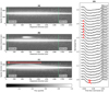 |
Fig. A.1 Moving ghost contaminating the spectral images of OB12. Panel A: a clear frame near the mid-transit. Panel B: a contaminated frame near the ingress of the transit. Panel C: stacking all contaminated frames showing the trace of ghost. The green dashed lines indicate the waveband for white-light curves. The red arrow indicates the moving direction of the ghostfrom the redder side to the bluer side. Panel D: raw spectroscopic light curves used in Sect. 3.2. The red dots correspond to the contaminated frames, which were removed in the spectroscopic light curve fitting. We note that the horizontal moire fringes shown in Panel A, B, and C were caused by the 500-kHz fast readout mode adopted in OB12 and were visually magnified due to a small figure size, which barely affected the stellar fluxes. |
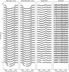 |
Fig. A.2 Spectroscopic light curve fitting of OB12. From left to right, the first panel: the raw light curves (circles) and the best-fit curves (solid lines); the second panel: the detrended light curves (circles) and the best-fit transit models (solid lines);the third panel: the extracted systematics (circles) and their GP models (solid lines); the fourth panel: the residuals. The points affected by the moving ghost have been removed. The curves were arbitrarily shifted for clarity. |
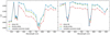 |
Fig. A.4 Bayesian evidence for different methods of spectroscopic light curve fitting for OB12 (left) and OB13 (right). The direct-fit method serves as a control group where the common modes are not removed in spectroscopic light curve fitting. |
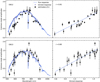 |
Fig. A.5 Flux-correlated amplitudes of common modes. The upper and lower panels correspond to the results of OB12 and OB13, respectively. Left panels: comparison between the common-mode amplitudes and flux response curves. Right panels: correlation between the common-mode amplitudes and binned flux responses. The blue dashed lines are linear regression models. The Pearson correlation coefficient is denoted as r. The flux response curves were arbitrarily rescaled for clarity but would not affect the correlation. |
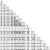 |
Fig. A.6 Posterior joint distributions of parameters for atmospheric retrieval. The contours indicate 39.3%, 86.5%, 98.9% (1- to 3-σ) credible intervals. The diagonal panels show the marginal distributions of corresponding parameters, in which the vertical dashed lines indicate the medians and 68.2% credible intervals. The specific values of posteriors are listed in Table 4. This figure is plotted utilizing the Python package corner (Foreman-Mackey 2016). |
References
- Alexoudi, X., Mallonn, M., von Essen, C., et al. 2018, A&A, 620, A142 [NASA ADS] [CrossRef] [EDP Sciences] [Google Scholar]
- Alexoudi, X., Mallonn, M., Keles, E., et al. 2020, A&A, 640, A134 [NASA ADS] [CrossRef] [EDP Sciences] [Google Scholar]
- Allard, F., Homeier, D., & Freytag, B. 2012, Phil. Trans. R. Soc. London, Ser. A, 370, 2765 [Google Scholar]
- Barstow, J. K., Aigrain, S., Irwin, P. G. J., & Sing, D. K. 2017, ApJ, 834, 50 [Google Scholar]
- Benneke, B., Knutson, H. A., Lothringer, J., et al. 2019, Nat. Astron., 3, 813 [Google Scholar]
- Berdyugina, S. V. 2005, Liv. Rev. Sol. Phys., 2, 8 [Google Scholar]
- Brown, T. M. 2001, ApJ, 553, 1006 [NASA ADS] [CrossRef] [Google Scholar]
- Buchner, J., Georgakakis, A., Nandra, K., et al. 2014, A&A, 564, A125 [NASA ADS] [CrossRef] [EDP Sciences] [Google Scholar]
- Cepa, J., Aguiar, M., Escalera, V. G., et al. 2000, SPIE Conf. Ser., 4008, 623 [Google Scholar]
- Chapman, G. A., Cookson, A. M., & Dobias, J. J. 1997, ApJ, 482, 541 [CrossRef] [Google Scholar]
- Chen, G., Guenther, E. W., Pallé, E., et al. 2017, A&A, 600, A138 [NASA ADS] [CrossRef] [EDP Sciences] [Google Scholar]
- Deibert, E. K., de Mooij, E. J. W., Jayawardhana, R., et al. 2019, AJ, 157, 58 [NASA ADS] [CrossRef] [Google Scholar]
- Deming, D., Wilkins, A., McCullough, P., et al. 2013, ApJ, 774, 95 [Google Scholar]
- Espinoza, N., & Jordán, A. 2015, MNRAS, 450, 1879 [Google Scholar]
- Evans, T. M., Sing, D. K., Wakeford, H. R., et al. 2016, ApJ, 822, L4 [NASA ADS] [CrossRef] [Google Scholar]
- Feroz, F., & Hobson, M. P. 2008, MNRAS, 384, 449 [NASA ADS] [CrossRef] [Google Scholar]
- Feroz, F., Hobson, M. P., & Bridges, M. 2009, MNRAS, 398, 1601 [NASA ADS] [CrossRef] [Google Scholar]
- Fisher, C., & Heng, K. 2018, MNRAS, 481, 4698 [Google Scholar]
- Foreman-Mackey, D. 2016, J. Open Source Softw., 1, 24 [Google Scholar]
- Foreman-Mackey, D., Agol, E., Ambikasaran, S., & Angus, R. 2017, AJ, 154, 220 [Google Scholar]
- Gibson, N. P., Aigrain, S., Roberts, S., et al. 2012, MNRAS, 419, 2683 [NASA ADS] [CrossRef] [Google Scholar]
- Gibson, N. P., Nikolov, N., Sing, D. K., et al. 2017, MNRAS, 467, 4591 [NASA ADS] [CrossRef] [Google Scholar]
- Gordon, I. E., Rothman, L. S., Hill, C., et al. 2017, J. Quant. Spectr. Rad. Transf., 203, 3 [Google Scholar]
- Greene, T. P., Line, M. R., Montero, C., et al. 2016, ApJ, 817, 17 [NASA ADS] [CrossRef] [Google Scholar]
- Hartman, J. D., Bakos, G. Á., Torres, G., et al. 2009, ApJ, 706, 785 [NASA ADS] [CrossRef] [Google Scholar]
- Herrero, E., Ribas, I., Jordi, C., et al. 2016, A&A, 586, A131 [NASA ADS] [CrossRef] [EDP Sciences] [Google Scholar]
- Johnson, L. J., Norris, C. M., Unruh, Y. C., et al. 2021, MNRAS, 504, 4751 [NASA ADS] [CrossRef] [Google Scholar]
- Kass, R. E., & Raftery, A. E. 1995, J. Am. Stat. Assoc., 90, 773 [Google Scholar]
- Kitzmann, D., & Heng, K. 2018, MNRAS, 475, 94 [NASA ADS] [CrossRef] [Google Scholar]
- Kreidberg, L. 2015, PASP, 127, 1161 [Google Scholar]
- Kreidberg, L., Bean, J. L., Désert, J.-M., et al. 2014, Nature, 505, 69 [Google Scholar]
- Line, M. R., Knutson, H., Deming, D., Wilkins, A., & Desert, J.-M. 2013, ApJ, 778, 183 [Google Scholar]
- MacDonald, R. J., Goyal, J. M., & Lewis, N. K. 2020, ApJ, 893, L43 [NASA ADS] [CrossRef] [Google Scholar]
- Madhusudhan, N., & Seager, S. 2009, ApJ, 707, 24 [NASA ADS] [CrossRef] [Google Scholar]
- Mallonn, M., Nascimbeni, V., Weingrill, J., et al. 2015, A&A, 583, A138 [NASA ADS] [CrossRef] [EDP Sciences] [Google Scholar]
- Mancini, L., Esposito, M., Covino, E., et al. 2018, A&A, 613, A41 [NASA ADS] [CrossRef] [EDP Sciences] [Google Scholar]
- Mandel, K., & Agol, E. 2002, ApJ, 580, L171 [Google Scholar]
- McCullough, P. R., Crouzet, N., Deming, D., & Madhusudhan, N. 2014, ApJ, 791, 55 [NASA ADS] [CrossRef] [Google Scholar]
- Nortmann, L., Pallé, E., Murgas, F., et al. 2016, A&A, 594, A65 [NASA ADS] [CrossRef] [EDP Sciences] [Google Scholar]
- Pinhas, A., Rackham, B. V., Madhusudhan, N., & Apai, D. 2018, MNRAS, 480, 5314 [Google Scholar]
- Pinhas, A., Madhusudhan, N., Gandhi, S., & MacDonald, R. 2019, MNRAS, 482, 1485 [Google Scholar]
- Pont, F., Sing,D. K., Gibson, N. P., et al. 2013, MNRAS, 432, 2917 [NASA ADS] [CrossRef] [Google Scholar]
- Rackham, B. V., Apai, D., & Giampapa, M. S. 2018, ApJ, 853, 122 [Google Scholar]
- Rackham, B. V., Apai, D., & Giampapa, M. S. 2019, AJ, 157, 96 [Google Scholar]
- Rasmussen, C. E., & Williams, C. K. I. 2006, Gaussian Processes for Machine Learning (Cambridge: The MIT Press) [Google Scholar]
- Rey, M., Nikitin, A. V., & Tyuterev, V. G. 2017, ApJ, 847, 105 [NASA ADS] [CrossRef] [Google Scholar]
- Richard, C., Gordon, I. E., Rothman, L. S., et al. 2012, J. Quant. Spec. Rad. Transf., 113, 1276 [NASA ADS] [CrossRef] [Google Scholar]
- Rosich, A., Herrero, E., Mallonn, M., et al. 2020, A&A, 641, A82 [NASA ADS] [CrossRef] [EDP Sciences] [Google Scholar]
- Sansonetti, J. E., & Martin, W. C. 2005, J. Phys. Chem. Ref. Data, 34, 1559 [NASA ADS] [CrossRef] [Google Scholar]
- Schlawin, E., Greene, T. P., Line, M., Fortney, J. J., & Rieke, M. 2018, AJ, 156, 40 [NASA ADS] [CrossRef] [Google Scholar]
- Seager, S., & Sasselov, D. D. 2000, ApJ, 537, 916 [Google Scholar]
- Sedaghati, E., Boffin, H. M. J., MacDonald, R. J., et al. 2017, Nature, 549, 238 [Google Scholar]
- Sing, D. K., Fortney, J. J., Nikolov, N., et al. 2016, Nature, 529, 59 [Google Scholar]
- Skilling, J. 2004, AIP Conf. Ser., 735, 395 [Google Scholar]
- Tashkun, S. A., & Perevalov, V. I. 2011, J. Quant. Spectr. Rad. Transf., 112, 1403 [NASA ADS] [CrossRef] [Google Scholar]
- Tennyson, J., & Yurchenko, S. 2018, Atoms, 6, 26 [CrossRef] [Google Scholar]
- Thorngren, D. P., Fortney, J. J., Murray-Clay, R. A., & Lopez, E. D. 2016, ApJ, 831, 64 [NASA ADS] [CrossRef] [Google Scholar]
- Tody, D. 1993, AIP Conf. Ser., 52, 173 [NASA ADS] [Google Scholar]
- Tsiaras, A., Waldmann, I. P., Zingales, T., et al. 2018, AJ, 155, 156 [NASA ADS] [CrossRef] [Google Scholar]
- Woitke, P., Helling, C., Hunter, G. H., et al. 2018, A&A, 614, A1 [NASA ADS] [CrossRef] [EDP Sciences] [Google Scholar]
- Wong, I., Benneke, B., Gao, P., et al. 2020, AJ, 159, 234 [NASA ADS] [CrossRef] [Google Scholar]
- Yan, F., Espinoza, N., Molaverdikhani, K., et al. 2020, A&A, 642, A98 [NASA ADS] [CrossRef] [EDP Sciences] [Google Scholar]
- Zacharias, N., Finch, C., Subasavage, J., et al. 2015, AJ, 150, 101 [Google Scholar]
- Zhang, M., & Chachan, Y. 2019, PLATON: PLanetary Atmospheric Transmission for Observer Noobs, Astrophysics Source Code Library, [record ascl:1903.014] [Google Scholar]
- Zhang, M., Chachan, Y., Kempton, E. M. R., Knutson, H. A., & Chang, W. H. 2020, ApJ, 899, 27 [CrossRef] [Google Scholar]
All Tables
Parameter estimates of atmospheric retrieval joint with other transmission spectra.
All Figures
|
Fig. 1 Stellar spectra of the target star HAT-P-12 (darker) and reference star GSC2 N130301284 (lighter) in OB12 (orange) and OB13 (blue). The dashed lines are passbands for spectroscopic light curves. The green solidlines indicate the D-lines of Na and K. The red-shaded band is strongly affected by the telluric O2 absorption. The stellar fluxes have been normalized and arbitrarily shifted for clarity. |
| In the text | |
|
Fig. 2 Joint white-light curve fitting of OB12 (left column) and OB13 (right column). Top panels: observed white-light curves (black dots), along with the best-fit curves (red lines) and systematics (green lines). Mid panels: detrended white-light curves (black dots) and the best-fit transit models (red lines). Bottom panels: residuals of light-curve fitting. |
| In the text | |
|
Fig. 3 Transmission spectra of OB12 (orange) and OB13 (blue). The red-shaded passband indicates the telluric O2 A-band. |
| In the text | |
|
Fig. 4 Posterior estimates of the orbital geometry parameters of HAT-P-12b compared with other literature values. The error bars indicate 1σ credible intervals. The contours indicate 1–3σ joint credible regions from nested sampling. |
| In the text | |
|
Fig. 5 Retrieved transmission spectra of HAT-P-12b. Upper panel: retrieved models composed of both model atmosphere and stellar contamination. Lower panel: transmission spectra and their retrieved models after stellar contamination correction. The model transmission spectra are wavelength-binned to a resolution of λ∕Δλ = 200. |
| In the text | |
|
Fig. 6 Major chemical species contributing to gas absorption features. Top panel: solid line is the median model shown in the lower panel of Fig. 5. The dashed line is the same atmospheric model but assuming zero abundance of H2O, CH4, and NH3. The transmission spectra of OB12 and OB13 have been corrected for stellar contamination. Middle panel: contributions of gas absorption to the transmission spectra. Bottom panel: posterior distributions of the major species’ volume mixing ratios. |
| In the text | |
|
Fig. 7 Transmission spectra of OB12 and OB13 recalculated with similar wavelength bins used in other research papers. |
| In the text | |
|
Fig. 8 Retrieval analysis joint with the transit depths presented in Yan et al. (2020) (LBT MODS) and Wong et al. (2020) (HST STIS G750; HST WFC3 G141; Spitzer IRAC). Upper panel: raw transmission spectra of the six data sets. Lower panel: shows the joint fit results with the effects of stellar contamination corrected for each data set. The green solid line is the median model with a resolution of λ∕Δλ = 200. The shaded areas indicate 68 and 95% credible intervals. The white dots are best-fit values calculated at the same wavelength bins as the corresponding data points. In the range of 0.5–1.0 μm, only the best-fit points corresponding to OSIRIS wavebands are displayed for clarity. |
| In the text | |
|
Fig. A.1 Moving ghost contaminating the spectral images of OB12. Panel A: a clear frame near the mid-transit. Panel B: a contaminated frame near the ingress of the transit. Panel C: stacking all contaminated frames showing the trace of ghost. The green dashed lines indicate the waveband for white-light curves. The red arrow indicates the moving direction of the ghostfrom the redder side to the bluer side. Panel D: raw spectroscopic light curves used in Sect. 3.2. The red dots correspond to the contaminated frames, which were removed in the spectroscopic light curve fitting. We note that the horizontal moire fringes shown in Panel A, B, and C were caused by the 500-kHz fast readout mode adopted in OB12 and were visually magnified due to a small figure size, which barely affected the stellar fluxes. |
| In the text | |
|
Fig. A.2 Spectroscopic light curve fitting of OB12. From left to right, the first panel: the raw light curves (circles) and the best-fit curves (solid lines); the second panel: the detrended light curves (circles) and the best-fit transit models (solid lines);the third panel: the extracted systematics (circles) and their GP models (solid lines); the fourth panel: the residuals. The points affected by the moving ghost have been removed. The curves were arbitrarily shifted for clarity. |
| In the text | |
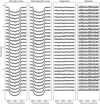 |
Fig. A.3 Same as Fig. A.2, but for light curves from the OB13 dataset. |
| In the text | |
|
Fig. A.4 Bayesian evidence for different methods of spectroscopic light curve fitting for OB12 (left) and OB13 (right). The direct-fit method serves as a control group where the common modes are not removed in spectroscopic light curve fitting. |
| In the text | |
|
Fig. A.5 Flux-correlated amplitudes of common modes. The upper and lower panels correspond to the results of OB12 and OB13, respectively. Left panels: comparison between the common-mode amplitudes and flux response curves. Right panels: correlation between the common-mode amplitudes and binned flux responses. The blue dashed lines are linear regression models. The Pearson correlation coefficient is denoted as r. The flux response curves were arbitrarily rescaled for clarity but would not affect the correlation. |
| In the text | |
|
Fig. A.6 Posterior joint distributions of parameters for atmospheric retrieval. The contours indicate 39.3%, 86.5%, 98.9% (1- to 3-σ) credible intervals. The diagonal panels show the marginal distributions of corresponding parameters, in which the vertical dashed lines indicate the medians and 68.2% credible intervals. The specific values of posteriors are listed in Table 4. This figure is plotted utilizing the Python package corner (Foreman-Mackey 2016). |
| In the text | |
Current usage metrics show cumulative count of Article Views (full-text article views including HTML views, PDF and ePub downloads, according to the available data) and Abstracts Views on Vision4Press platform.
Data correspond to usage on the plateform after 2015. The current usage metrics is available 48-96 hours after online publication and is updated daily on week days.
Initial download of the metrics may take a while.