| Issue |
A&A
Volume 656, December 2021
|
|
|---|---|---|
| Article Number | A106 | |
| Number of page(s) | 14 | |
| Section | Cosmology (including clusters of galaxies) | |
| DOI | https://doi.org/10.1051/0004-6361/202141744 | |
| Published online | 09 December 2021 | |
Dark Energy Survey Year 3 Results: Galaxy mock catalogs for BAO analysis
1
Institute of Theoretical Astrophysics, University of Oslo, PO Box 1029, Blindern, 0315 Oslo, Norway
e-mail: This email address is being protected from spambots. You need JavaScript enabled to view it.
2
Institut d’Estudis Espacials de Catalunya (IEEC), 08034 Barcelona, Spain
3
Institute of Space Sciences (ICE, CSIC), Campus UAB, Carrer de Can Magrans, s/n, 08193 Barcelona, Spain
4
Center for Cosmology and Astro-Particle Physics, The Ohio State University, Columbus, OH 43210, USA
5
Department of Physics, The Ohio State University, Columbus, OH 43210, USA
6
Max-Planck-Institut für Astrophysik, Karl-Schwarzschild Str. 1, 85741 Garching, Germany
7
Instituto de Astrofisica de Canarias, 38205 La Laguna, Tenerife, Spain
8
Laboratório Interinstitucional de e-Astronomia – LIneA, Rua Gal. José Cristino 77, Rio de Janeiro, RJ 20921-400, Brazil
9
Universidad de La Laguna, Dpto. Astrofísica, 38206 La Laguna, Tenerife, Spain
10
Instituto de Fisica Teorica UAM/CSIC, Universidad Autonoma de Madrid, 28049 Madrid, Spain
11
Institute of Cosmology and Gravitation, University of Portsmouth, Dennis Sciama Building, Burnaby Road, Portsmouth PO1 3FX, UK
12
School of Physics and Astronomy, Sun Yat-sen University, 2 Daxue Road, Tangjia, Zhuhai 519082, PR China
13
Instituto de Física Teórica, Universidade Estadual Paulista, São Paulo, Brazil
14
ICTP South American Institute for Fundamental Research, São Paulo, Brazil
15
Centro de Investigaciones Energéticas, Medioambientales y Tecnológicas (CIEMAT), Madrid, Spain
16
Port d’Informació Científica (PIC), Campus UAB, C. Albareda s/n, 08193 Bellaterra, Barcelona, Spain
17
Institut de Física d’Altes Energies (IFAE), The Barcelona Institute of Science and Technology, Campus UAB, 08193 Bellaterra, Barcelona, Spain
18
Jet Propulsion Laboratory, California Institute of Technology, 4800 Oak Grove Dr., Pasadena, CA 91109, USA
19
Instituto de Física Gleb Wataghin, Universidade Estadual de Campinas, 13083-859 Campinas, SP, Brazil
20
Department of Astronomy/Steward Observatory, University of Arizona, 933 North Cherry Avenue, Tucson, AZ 85721-0065, USA
21
Departamento de Física Matemática, Instituto de Física, Universidade de São Paulo, CP 66318, São Paulo, SP 05314-970, Brazil
22
Laboratório Interinstitucional de e-Astronomia, Rua General José Cristino, 77, São Cristóvão, Rio de Janeiro, RJ 20921-400, Brazil
23
Fermi National Accelerator Laboratory, PO Box 500, Batavia, IL 60510, USA
24
CNRS, UMR 7095, Institut d’Astrophysique de Paris, 75014 Paris, France
25
Sorbonne Universités, UPMC Univ. Paris 06, UMR 7095, Institut d’Astrophysique de Paris, 75014 Paris, France
26
Department of Physics & Astronomy, University College London, Gower Street, London WC1E 6BT, UK
27
Center for Astrophysical Surveys, National Center for Supercomputing Applications, 1205 West Clark St., Urbana, IL 61801, USA
28
Department of Astronomy, University of Illinois at Urbana-Champaign, 1002 W. Green Street, Urbana, IL 61801, USA
29
Physics Department, 2320 Chamberlin Hall, University of Wisconsin-Madison, 1150 University Avenue Madison, Madison, WI 53706-1390, USA
30
Jodrell Bank Center for Astrophysics, School of Physics and Astronomy, University of Manchester, Oxford Road, Manchester M13 9PL, UK
31
University of Nottingham, School of Physics and Astronomy, Nottingham NG7 2RD, UK
32
Astronomy Unit, Department of Physics, University of Trieste, Via Tiepolo 11, 34131 Trieste, Italy
33
INAF-Osservatorio Astronomico di Trieste, Via G. B. Tiepolo 11, 34143 Trieste, Italy
34
Institute for Fundamental Physics of the Universe, Via Beirut 2, 34014 Trieste, Italy
35
Observatório Nacional, Rua Gal. José Cristino 77, Rio de Janeiro, RJ 20921-400, Brazil
36
Department of Physics, University of Michigan, Ann Arbor, MI 48109, USA
37
Department of Astronomy and Astrophysics, University of Chicago, Chicago, IL 60637, USA
38
Kavli Institute for Cosmological Physics, University of Chicago, Chicago, IL 60637, USA
39
Santa Cruz Institute for Particle Physics, Santa Cruz, CA 95064, USA
40
Department of Astronomy, University of Michigan, Ann Arbor, MI 48109, USA
41
Department of Physics, Stanford University, 382 Via Pueblo Mall, Stanford, CA 94305, USA
42
Kavli Institute for Particle Astrophysics & Cosmology, Stanford University, PO Box 2450, Stanford, CA 94305, USA
43
SLAC National Accelerator Laboratory, Menlo Park, CA 94025, USA
44
School of Mathematics and Physics, University of Queensland, Brisbane, QLD 4072, Australia
45
Faculty of Physics, Ludwig-Maximilians-Universität, Scheinerstr. 1, 81679 Munich, Germany
46
Center for Astrophysics | Harvard & Smithsonian, 60 Garden Street, Cambridge, MA 02138, USA
47
Australian Astronomical Optics, Macquarie University, North Ryde, NSW 2113, Australia
48
Lowell Observatory, 1400 Mars Hill Rd, Flagstaff, AZ 86001, USA
49
Departamento de Física Matemática, Instituto de Física, Universidade de São Paulo, CP 66318, São Paulo, SP 05314-970, Brazil
50
George P. and Cynthia Woods Mitchell Institute for Fundamental Physics and Astronomy, and Department of Physics and Astronomy, Texas A&M University, College Station, TX 77843, USA
51
Institució Catalana de Recerca i Estudis Avançats, 08010 Barcelona, Spain
52
Institute of Astronomy, University of Cambridge, Madingley Road, Cambridge CB3 0HA, UK
53
Department of Physics and Astronomy, University of Waterloo, 200 University Ave W, Waterloo, ON N2L 3G1, Canada
54
Perimeter Institute for Theoretical Physics, 31 Caroline St. North, Waterloo, ON N2L 2Y5, Canada
55
Department of Astrophysical Sciences, Princeton University, Peyton Hall, Princeton, NJ 08544, USA
56
School of Physics and Astronomy, University of Southampton, Southampton SO17 1BJ, UK
57
Computer Science and Mathematics Division, Oak Ridge National Laboratory, Oak Ridge, TN 37831, USA
58
Institute of Cosmology and Gravitation, University of Portsmouth, Portsmouth PO1 3FX, UK
59
Max Planck Institute for Extraterrestrial Physics, Giessenbachstrasse, 85748 Garching, Germany
60
Universitäts-Sternwarte, Fakultät für Physik, Ludwig-Maximilians Universität München, Scheinerstr. 1, 81679 München, Germany
Received:
8
July
2021
Accepted:
28
September
2021
Abstract
The calibration and validation of scientific analysis in simulations is a fundamental tool to ensure unbiased and robust results in observational cosmology. In particular, mock galaxy catalogs are a crucial resource to achieve these goals in the measurement of baryon acoustic oscillation (BAO) in the clustering of galaxies. Here we present a set of 1952 galaxy mock catalogs designed to mimic the Dark Energy Survey Year 3 BAO sample over its full photometric redshift range 0.6 < zphoto < 1.1. The mocks are based upon 488 ICE-COLA fast N-body simulations of full-sky light cones and were created by populating halos with galaxies, using a hybrid halo occupation distribution – halo abundance matching model. This model has ten free parameters, which were determined, for the first time, using an automatic likelihood minimization procedure. We also introduced a novel technique to assign photometric redshift for simulated galaxies, following a two-dimensional probability distribution with VIMOS Public Extragalactic Redshift Survey data. The calibration was designed to match the observed abundance of galaxies as a function of photometric redshift, the distribution of photometric redshift errors, and the clustering amplitude on scales smaller than those used for BAO measurements. An exhaustive analysis was done to ensure that the mocks reproduce the input properties. Finally, mocks were tested by comparing the angular correlation function w(θ), angular power spectrum Cℓ, and projected clustering ξp(r⊥) to theoretical predictions and data. The impact of volume replication in the estimate of the covariance is also investigated. The success in accurately reproducing the photometric redshift uncertainties and the galaxy clustering as a function of redshift render this mock creation pipeline as a benchmark for future analyses of photometric galaxy surveys.
Key words: catalogs / large-scale structure of Universe / galaxies: distances and redshifts / Galaxy: halo / methods: numerical
© ESO 2021
1. Introduction
Over recent years, a large international effort has been focused on constraining the dark energy properties, measuring the cosmological parameters with high accuracy, and testing the Lambda cold dark matter (ΛCDM) paradigm. This led to the development of new techniques and data combinations that allow tighter constraints: cosmic microwave background (CMB); Type Ia supernovae (SNe Ia); galaxy clustering (GC); weak lensing (WL); baryon acoustic oscillation (BAO); etc. Especially in recent years, BAO (Peebles & Yu 1970; Sunyaev & Zeldovich 1970) has become a powerful alternative to building the Hubble diagram, which now allows one estimate cosmological parameters by itself (Percival et al. 2007; Beutler et al. 2011; Alam et al. 2021).
Most of the probes mentioned before require the measurement of redshifts with high fidelity, giving more significance to spectroscopic surveys (e.g., the WFC3 Infrared Spectroscopic Parallel Survey – WISP1, Baryon Oscillation Spectroscopic Survey – BOSS2, Euclid3, Wide-Field Infrared Survey Telescope – WFIRST4, Dark Energy Spectroscopic Instrument – DESI5). However, photometric surveys have some advantages over the spectroscopic ones. In particular, every observed galaxy can be used in the cosmological analysis although in practice is necessary to select a galaxy population that presents a prominent spectral feature that can be captured with broadband filters. Besides, many successful techniques are used to estimate true redshifts given observed photometric redshifts (photo-z) within a given uncertainty. Then, the statistical power makes imaging surveys almost as competitive as spectroscopic surveys in the measurement of galaxy clustering. One example of these techniques is the Directional Neighbourhood Fitting (DNF, De Vicente et al. 2016), which stands out as one of the most robust and accurate determinations of photo-z, and is thus used in several photometric surveys (see e.g., Drlica-Wagner et al. 2018; Sevilla-Noarbe et al. 2021; Euclid Collaboration 2020). The Dark Energy Survey (DES)6 is a badge example. DES has mapped the southern sky for six years covering an area of ∼5000 deg2 and has recorded data from a few hundred million distant galaxies. These numbers will be pushed even beyond by future projects (e.g., the Legacy Survey of Space and Time – Rubin LSST7, Spectro-Photometer for the History of the Universe, Epoch of Reionization, and Ices Explorer – SPHEREx8).
For the large data sets that these projects produce, the calibration and replication of scientific analysis in simulations previous to unblinding (procedure explained below), is a fundamental tool to ensure unbiased and robust results. This task requires the fulfillment of two requirements: (i) a realistic simulation of the observed cosmological volume with a final galaxy catalog that mimics the data and (ii) a large number of realizations varying the initial conditions that allows a full control of statistical uncertainties. The negative effects of introducing simulated volume replications to achieve the first requisite should not be underestimated. For example, the consequence of over-estimation of the covariances was found in the mocks used for this work. Accomplishing the second requirement by using pure N-body simulations is computationally impossible when the number of needed realizations is hundreds or thousands. Using approximate methods allows to have the desired number of runs with less computational resources (see e.g., Coles & Jones 1991; Scoccimarro & Sheth 2002; Koda et al. 2016; Avila et al. 2015; Chuang et al. 2015a; Izard et al. 2018). All these methods reduce the resolution of the simulation on small scales in exchange for computing speed. But when we focus our study on BAO scales, as the purpose of this work, it has been shown that the accuracy of these approximate methods is more than sufficient for a precise analysis (Chuang et al. 2015b; Lippich et al. 2019; Blot et al. 2021). For example, Izard et al. (2016) demonstrates that the ICE-COLA method yields a matter power spectrum within 1% for k ≲ 1 h Mpc−1 and a halo mass function within 5% of those in the N-body. Nowadays, all cosmological surveys need to develop their own galaxy mock catalogs in order to properly simulate the characteristics of the data. BOSS, eBOSS and the first year of DES data (DES Y1) for example have designed their own mocks (Manera et al. 2013; Chuang et al. 2015a,b; Kitaura et al. 2016; Avila et al. 2018; Zhao et al. 2021). The BAO analysis using the first three years of DES data (DES Y3) is structured in three papers: Carnero Rosell et al. (2022) presents a systematics analysis of the galaxy sample for DES Y3 BAO measurement, this work describes the simulations used in the analysis and the main DES Y3 BAO paper presents the angular distance constrains and cosmology in DES Collaboration (2021). An analogous work was made for DES Y1: the DES Y1 sample was presented in Crocce et al. (2019), a description of the mocks was shown in Avila et al. (2018) and DES Collaboration (2019) as the main DES Y1 BAO paper including a ∼4% precision DA measurement. In this case, the work was accompanied by several method papers (Chan et al. 2018; Ross et al. 2017; Camacho et al. 2019).
A common process in the analysis of new Surveys data release is to blind the data in certain ways. The implementation of a rigorous process of unblinding can reduce or eliminate confirmation bias. A strict blinding strategy has been applied to this work. The final set of mocks, presented here, were completed before computing α (BAO shift parameter) on the final data vector, and before plotting the angular two-point correlation function or clustering Cℓ of the DES Y3 sample. Only three pre-unblinding values of the angular clustering on scales lower than one degree (unused for the BAO analysis) were provided to calibrate the clustering amplitude of the mocks. Once the mocks were done and the data passed through the rigorous process of unblinding we could compare the clustering both in configuration and harmonic space of the mocks with the final post-unblinding measurements of the data. We refer the interested reader to DES Collaboration (2021) for more details about the unblinding process of the data.
This paper is arranged as follows. In Sect. 2 we briefly describe the reference sample. Then, Sect. 3 describes the main features of the used dark matter halo catalogs. On the one hand, we present the fast simulation used to perform the mocks for the analysis, and on the other hand, our benchmark pure N-body simulation. In Sect. 4 we detail step by step the process we followed to create our galaxy catalogs, which match the main properties of the data. One of the most important aspects of our pipeline is the automatic calibration, which is exhaustively detailed in Sect. 5. After describing how the mocks are created, in Sect. 6 we compare them with the real data and theoretical models in terms of covariance matrices and clustering measurements, both in angular configuration space and angular harmonic space. Additionally, in Sect. 7 we investigate the effect of replicated structures in the mocks. Finally, we conclude in Sect. 8 with our summary and conclusions.
2. Reference data
The BAO analysis for the DES Y3 data set is based on the Y3 GOLD catalog (Sevilla-Noarbe et al. 2021), which contains nearly 390 million objects, with a depth reaching S/N ∼ 10 for extended objects up to i < 22.3 (AB), and top-of-the-atmosphere photometric accuracy under 3 mmag. This data set has been compiled from the coaddition of nearly 40 000 exposures in the grizY optical and near-infrared bands taken during the first three years of observations. It used the DECam instrument (Flaugher et al. 2015) from the Blanco Telescope in Cerro Tololo (Chile) and covers 5000 deg2 of the southern hemisphere.
The catalog includes positional, photometric, and morphological information, using a multi-epoch, multi-band fitting procedure of the object’s shape in every exposure where the object is present (the Single Object Fitting, or SOF, method). This is the basis of all the measurements of the object mentioned before. In addition, the Y3 GOLD catalog contains flagging information to assess the quality of the measured object, and ancillary survey information about low-quality regions in the sky, and survey properties in general (seeing, airmass, etc).
From the Y3 GOLD, we select a sample of red galaxies used to measure the BAO scale, with a color selection similar to the DES Y1 analysis presented in Crocce et al. (2019). The DES Y3 selection shows an increase in the number density of galaxies (due to improvements on the DESDM9 reduction), which allows us to extend the redshift range of the analysis to photometric redshift zphoto < 1.1 with i < 22.3 (AB). The selection applied to create the sample is summarized in Table 1 (details can be found in Carnero Rosell et al. 2022).
Selection process to create the BAO sample in DES Y3.
Furthermore, the footprint mask is selected accordingly removing regions with depth less than 22.3, plus additional quality cuts explained in the aforementioned references. We use all HEALPix maps with NSIDE=4096 found in the online release10. In Fig. 1, we show the angular distribution of the BAO footprint, covering 4108.47 deg2.
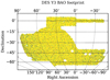 |
Fig. 1. DES Y3 sample footprint, covering 4108.47 deg2 of the southern sky. |
One of the most critical aspects of any photometric analysis is the measurement of the redshift. For the sample, we characterize the N(z) (the true redshift distribution) in each tomographic bin using the “VIMOS Public Extragalactic Redshift Survey” (Guzzo et al. 2014, VIPERS) catalog as a reference, since it is a complete sample from redshift above z = 0.5 up to i = 22.5 (AB). VIPERS observed in two fields, named W1 and W4, both overlapping DES. The total overlap area is 16.324 deg2 This provides, after several selection processes described in Carnero Rosell et al. (2022), a final sample of 8362 galaxies with spectroscopic redshift, zVIPERS, available for redshift calibration. Carnero Rosell et al. (2022) use VIPERS to validate the performance of the photometric redshift (called Z_MEAN in the DES catalogs) and to estimate the true redshift (Z_MC) distribution of the DES Y3 sample. DNF predicts Z_MEAN as the best-value in the fitted hyper-plane and also defines Z_MC as the closest friend. In this work, we use these overlapping galaxies for the opposite purpose, assigning zphoto to the simulated galaxies. In other words, we re-sample the zspec vs zphoto diagram found from VIPERS to assign zphoto to mock galaxies.
3. Halo light cone catalogs
In this section, we describe the halo catalogs from dark matter simulations used in this paper. We start by describing the ICE-COLA fast simulations and then our benchmark pure N-body simulation, MICE Grand Challenge. It is important to make clear that both sets of simulations share the same cosmology, mass resolution, and halos found with a Friends of Friends algorithm.
3.1. ICE-COLA fast simulations
To build a large number of mocks we use a set of 488 fast N-body simulations generated with the ICE-COLA code (Izard et al. 2016). The COmoving Lagrangian Acceleration (COLA) method solves for the evolution of the matter density field using second-order Lagrangian Perturbation Theory (2LPT) combined with a Particle-Mesh (PM) solver to integrate the particle orbits at small scales, where 2LPT start to deviate from the full N-body solution (Tassev et al. 2013; Koda et al. 2016). The ICE-COLA code extends on this method to produce on-the-fly light cone halo catalogs and weak lensing maps (Izard et al. 2018).
The simulations use 20483 particles in a box of size of 1536 Mpc h−1 to match the mass resolution of the MICE Grand Challenge simulation (see Sect. 3.2). Here we use the optimal code parameters found in Izard et al. (2016), namely 40 time-steps, a starting redshift of zini = 19 and a PM grid of 27 times the number of particles. Halos are found with a Friends of Friends (FOF) algorithm with linking length b = 0.2. We refer the interested readers to Koda et al. (2016) and Izard et al. (2016) for more complex analysis and thorough validation of the method.
It is important to know the limitations of fast simulations to be able to use them in the range of scales where they agree with N-body, but also (moderately) beyond those scales with a systematic error that can be quantified (i.e, under control).
3.2. MICE Grand Challenge simulation
As was mentioned before, it is really important to validate the range of scales where we can trust fast simulations. In our case, we use the MICE Grand Challenge11 (Fosalba et al. 2015b,a; Crocce et al. 2015, MICE hereafter), simulation as the benchmark N-body run. MICE is an all-sky light cone N-body simulation evolving 40963 dark-matter particles in a ∼29 Gpc3 h−3 comoving volume. The assumed cosmology corresponds to the best-fit of WMAP five-year data (Komatsu et al. 2009). This is consistent with a flat ΛCDM model with Ωm = 0.25, ΩΛ = 0.75, Ωb = 0.044, ns = 0.95, σ8 = 0.8 and h = 0.7.
As our reference simulation, its cosmological parameters are also used for our ICE-COLA runs, where only the initial condition changes among the 488 fast simulations. An exhaustive validation of the simulations used here has been done in Izard et al. (2016), finding a matter power spectrum within 1% for k ≲ 1 h Mpc−1 and demonstrating that ICE-COLA fast simulation can perfectly be used for BAO purposes. In Fig. 2, we compare the halo masses and the clustering for redshift z = 0.5 (blue) and z = 1 (red). The top panel shows the ratio between the MICE and the ICE-COLA halo mass function, the lowest halo mass plotted here correspond to the mass limit of the ICE-COLA mock used in this paper, 1.46 × 10¹² M⊙ (50 particles). Both simulations are consistent, as was found in Izard et al. (2016), within an accuracy of ∼5%. The bottom panel of Fig. 2 shows the ratio between the MICE and the ICE-COLA angular two-point correlation function (ACF). In this case, the clustering is calculated using halos with more than 50 particles in a full-octant comoving output shell of width 125 Mpc and 166 Mpc for redshift z = 0.5 and z = 1, respectively. This threshold of 50 particles is not set deliberately but is a resulting minimum number of particles of the halos of the mocks presented in this work. For clustering, the accuracy is within ∼5% up to scales of one degree. For higher angular distances the error increase, especially for redshift z = 1 where these scales correspond to larger 3D distances.
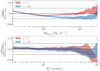 |
Fig. 2. Top panel: ratio of the Halo Mass Function between MICE and ICE-COLA. Blue for redshift z = 0.5 and red for z = 1. Shaded areas correspond to the standar deviation of the 488 ICE-COLA runs. Bottom panel: ratio between the MICE and the ICE-COLA ACF for a sample of halos with Mhalo > 1.46 × 10¹² M⊙. |
4. Galaxy light cone catalogs
With the simulations and the corresponding ICE-COLA halo catalogs presented in the previous section, we can start now by describing, step by step, the mechanism used to construct a galaxy mock beginning with a halo catalog. Some of our recipes described below closely follows Carretero et al. (2015) and we use a similar hybrid Halo Occupation Distribution – Halo Abundance Matching model modeling strategy presented by Avila et al. (2018) in the analysis of the DES Y1 data release. Before going into the details, it is important to remark that simulated box replications are needed to have light cones reaching higher redshifts than 0.6 (corresponding limiting redshift if we set the light cone origin at the center of a box-size of 1 536 Mpc h−1) and covering the DES Y3 footprint. Four boxes on each Cartesian direction are needed (a total of 64 simulated boxes) to create a full-sky light cone up to redshift ∼1.4. The implications that these replications have on the analysis are discussed in more detail in Sect. 7.
Here, we create a mock of galaxies for BAO analysis from a halo catalog of a fast simulation. However, the described procedure can be applied to any sort of halo catalog to mimic any kind of galaxies samples. A key aspect that makes this pipeline successful is the inclusion of an automatic calibration, as discussed in Sect. 5.
4.1. Halo occupation distribution
The relation between galaxies and halos is not univocal, as one halo can harbor more than one galaxy. Furthermore, the more massive the halo the higher the number of galaxies it has, reaching quantities of hundreds of galaxies in a single halo. The halo occupation distribution (HOD; Jing et al. 1998; Benson et al. 2000; Seljak 2000), describes the relation between halos and galaxies, in terms of several parameters. In other words, the HOD tells us how many galaxies a halo of a given mass has on average, ⟨N|Mhalo⟩.
Two different functions are needed to describe the HOD of a sample of galaxies. One for the central galaxies and another for satellites as they model clustering on different scales in the halo model. Centrals shape large scales (halo-halo correlations) and satellite small scales (intra-halo correlations). The complexity of the function can be as high as desired, in order to match the behavior of the sample with higher accuracy. We focus here on the large-scale structure, leaving aside a complex function that would allow us to model the small scales. Therefore, we assign to each halo, one central galaxy
 (1)
(1)
and a number of satellite galaxies following a Poisson distribution with mean
 (2)
(2)
where Mhalo is the mass of the halo, and M1 is a free HOD parameter. This simple HOD is used to populate all halos with galaxies in the light cone. However, the particular sample selection is a sub sample of this generic HOD assignment. Therefore, the final values of Ncent(Mhalo) and Nsat(Mhalo) that compose the sample of the mocks differs from the expression defined on Eqs. (1) and (2).
Once Ncent and Nsat values are determined, the next step is to populate the halos with galaxies following these HOD quantities. One central galaxy is placed in the center of each halo and the velocity is assumed to be equal to its host halo. On the other hand, satellites galaxies are distributed inside the halo following a spherical NFW (Navarro et al. 1996) profile. Concentrations, needed to model the NFW density profile, are taken from Cooray & Sheth (2002) where the inputs are the mass and redshift of halos. We also model the velocity of galaxies with simplistic assumptions, using a simple Gaussian distribution centered at the velocity of the host halo and assuming a standard deviation proportional to the velocity dispersion of it (Sheth & Diaferio 2001; Carretero et al. 2015).
This first free parameter, M1, allows to control the clustering: by increasing the parameter, we undersample the most massive halos decreasing the linear bias. It also introduces a 1-halo term that fades away as we increase M1. More details can be found in Avila et al. (2018). Figure 3 shows the evolution of M1 over the five tomographic bins where we assume a linear interpolation among these values. In Sect. 5 is explained in detail how these values are obtained.
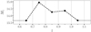 |
Fig. 3. Evolution of the first HOD free parameter M1. One value for each tomographic bin. Dashed line correspond to the interpolation assumed for all the redshift range. |
At this point, we already have a general galaxy catalog with positions and velocities, made by populating all halos on the light cone. The next step is to introduce a second free parameter by setting pseudo luminosities. This second HOD parameter allows setting a sample by selecting only high luminosity galaxies from the general catalog.
4.2. Pseudo-luminosity assignment
The best tracers for BAO signal are brightest galaxies (see e.g., Comparat et al. 2013) and they represent a few percent of the total number of galaxies. Not all galaxies resulting from the previous step 4.1 will enter into our selection to perform the BAO analysis. Therefore, this step is needed to select that few percent of galaxies.
An efficient way to select the tracers of our mocks is by assigning a pseudo luminosity lp to all galaxies and then selecting the most luminous ones. To set the luminosities we rely on the halo abundance matching (HAM) techniques (Kravtsov et al. 2004; Conroy et al. 2006; Guo et al. 2010), where it is assumed that the most massive (luminous) galaxy lives in the most massive halo, the second most massive galaxy lives in the second most massive halo, and so on. On top of the mean (deterministic) relation between mass and luminosity assumed in the AM technique, we add some scattering to make this matching closer to observations. We model lp with a Gaussian scatter around the halo mass Mhalo in logarithmic scales:
 (3)
(3)
where ΔLM is our second free parameter which controls the amount of scatter. We note that lp is modeled in arbitrary scales. The purposes of defining a luminosity for galaxies are two:
-
It allows one to match the abundance and redshift distribution of data by selecting the most luminous galaxies. More details on Sect. 4.3.
-
Its definition, and therefore the introduction of the second free parameter ΔLM, also influences the clustering. As we decrease this value, lower mass halos go out of our selection and higher mass halos enter it, effectively increasing the bias.
Figure 4 shows the evolution of this scatter parameter ΔLM as a function of redshift. In the same way as M1, we assume for ΔLM one value for each tomographic bin and applying linear interpolation among these values as a function of redshift. The modeling explained in this subsection follows the same procedure used in Avila et al. (2018). As was mentioned earlier, in Sect. 5 it is explained how these values are obtained.
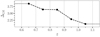 |
Fig. 4. Evolution of the second HOD parameter ΔLM. One value for each tomographic bin. Dashed line corresponds to the interpolation assumed for all redshift range. |
4.3. Photometric redshifts
This is perhaps one of the most dedicated and challenging steps of the mock creation pipeline. For the ICE-COLA mocks we know the true redshift and we need to model the observed one for each simulated galaxy, contrary to what happens for observations. DES is a photometric survey, therefore the measurement of the redshift has a precision much lower than spectroscopic surveys. For example, Carnero Rosell et al. (2022) show that the dispersion on the photo-z for the DES Y3 sample is σ68 = 0.054 on average for the five tomographic bins. σ68 is defined as the value such as 68 per cent of the galaxies have |zphoto − zspec|/(1 + zspec) < σ68. These uncertainties must be modeled in the simulation to have consistent clustering measurements.
Each galaxy in DES has an observed photometric redshift Z_MEAN, derived from the magnitude measured in each filter. In addition, as was explained in Sect.2, there is a small sample of 8362 galaxies for which we also have the true spectroscopic redshifts from VIPERS (zVIPERS). The combination of using DES and VIPERS result in our mocks matching the abundance of DES Y3 BAO galaxies n(Z_MEAN) and the redshift distribution N(zVIPERS) on each tomographic bin of these galaxies present in both surveys.
We start by dividing the interval Z_MEAN = [0.6, 1.1] into L thin bins of with ΔZ_MEAN = 0.01. Then, according to the data, we can express the number of galaxies each l bin has as n(Z_MEANl). This is the first condition we want to accomplish with the mocks: match the abundance of each l thin photometric bin.
Secondly, we select M spectroscopic bins of width ΔzVIPERS = 0.025, here bins are thicker because of the smaller number of VIPERS galaxies. Then, we can determine the probability of having a galaxy in a given pair of bins (l,m) as  . It is important to remark that this matrix is built only using those DES galaxies which have a zVIPERS. Mocks need to satisfy this 2D probability distribution P(Z_MEAN, zVIPERS) and, at the same time, match the abundance of galaxies n(Z_MEAN). By combining both, the number of galaxies an ICE-COLA mock should have at a given pair of bins(l,m) can be calculated as
 (4)
(4)
The assignment of photometric redshifts zphoto to galaxies in mocks is then performed in two steps. Firstly, we separate the simulated galaxies into L and M bins and assigning zphoto by following the distribution P(Z_MEAN, zVIPERS). And finally, we choosing from each (l,m) pair of bins the Al, m most luminous galaxies, given the luminosities defined on Eq. (3). The Fig. 5 shows the resulting n(zphoto) for the mocks compared with data. Gray histograms correspond to DES Y3 sample and red points with error bars represent the mocks. The agreement is almost perfect, as expected given that it is done by construction. On the other hand, to achieve a good match on redshift distribution N(zspec) for each tomographic bin is normally not so easy, but with this technique, it is also achieved by construction. This is shown in Fig. 6 where filled green histograms correspond to VIPERS data while the black line denotes distribution for DES Y3. As in Fig. 5 red points represent the average of the mocks and error bars correspond to the maximum and minimum. The goal here was to assign zphoto in such a way that it gives a redshift distribution N(zspec) on each tomographic bin matching those of the DES Y3 BAO galaxies present in VIPERS.
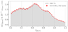 |
Fig. 5. Photometric redshift distribution of data and mocks. Gray histogram corresponds to DES Y3 sample. Red points represent the average over the 1952 ICE-COLA mocks and error bars denote the maximum and minimum. |
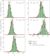 |
Fig. 6. True redshift zspec distribution in each tomographic bin. Green filled histograms correspond to VIPERS, black lines represent the distribution for Y3 data and red point are the average over the 1952 ICE-COLA mocks, while error bars correspond to the maximum and minimum. Histograms are normalized to have an integral of unity. |
Some important quantities must be compared for a correct photo-z validation, and are evaluated on each tomographic bin. These are the mean redshift ( ), the width of the N(z) (W68, opposed to the dispersion), and the dispersion on the photo-z (σ68). The performance of these quantities in the mocks are analyzed against VIPERS galaxies (for those we have both Z_MEAN and zVIPERS) in Fig. 7. The top panel shows the difference in
  between the estimated true redshift for DES Y3 sample (Z_MC, dotted black) and ICE-COLA mocks (red) against VIPERS (zVIPERS). In the medium and bottom panel, we present the evolution of σ68 and W68 as a function of
  for each sample, respectively. In all three quantities studied here, the agreement between VIPERS and the mocks is very satisfactory, showing a difference within 1%. Of course, our method to assign zphoto by construction should show a perfect match, with zero uncertainties. However, the small differences we see in Fig. 7 come from the fact that the sample of VIPERS galaxies (8362) is not fully representative of the 2D space zphoto-zspec. We want to stress that the difference between zVIPERS and Z_MC represents an estimation of the uncertainty we have on the redshifts, and hence the precision of the mocks is well below those uncertainties. We refer the interested reader to Carnero Rosell et al. (2022) for details on the performance of using VIPERS as a training sample for photo-z validation and true redshift assignment of the sample.
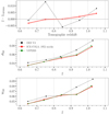 |
Fig. 7. Basic metrics for the photo-z validation on each tomographic bin. From top to bottom: difference between |


This step is different from what was done for DES Y1 by Avila et al. (2018). Here we use an “exact” method which may propagate noise while Avila et al. (2018) used an “analytical” procedure (fitting a double skewed Gaussian) which may miss some photo-z features.
4.4. Masking
Finally, our last step is to create galaxy mocks with the same footprint as the data. The angular mask of the DES Y3 sample, described in Sect 2, has an area of 4108.47 deg2 and final ICE-COLA mocks must have the same characteristics with the same HEALPix resolution NSIDE=4096 as the data mask. To satisfy this and at the same time be efficient in creating as many catalogs as possible, four masks are placed on each full-sky light cone. This allows us to go from having 488 ICE-COLA runs to having 1952 BAO galaxy mocks at the end, quadrupling the number of simulations. This is illustrated in Fig. 8 where four DES Y3 BAO footprints are placed, without overlapping, in a full-sky light cone. Although this configuration of masks maximizes the number of mocks, on Sect. 7 we return to this and analyze the negative implications it has on the covariance matrix.
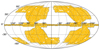 |
Fig. 8. Configuration of four DES Y3 BAO footprints on a full-sky. Mask are constructed with HEALPix assuming a resolution NSIDE=4096. |
5. Calibration
The pipeline used to generate the BAO mocks contains two free parameters per tomographic bin, M1 and ΔLM, as detailed in the previous section. This amounts to a total of ten free parameters that should be varied altogether to minimize the difference between the measurements and the mocks. In more detail, we want to minimize the discrepancy between the measured w(θ) and the one obtained from the mocks. Let us emphasize that “w(θ)” in this section refers to the measurement of the angular correlation function calculated only for the three pre-unblinding angular apertures θ = [0.58, 0.75, 0.92]. The main problem that we have to address is that we cannot obtain w(θ) from the mocks without first specifying the values of these parameters, generating the mocks, and measuring the observable quantity. If the parameter space were small we could attempt to vary the parameters one at a time, run a few cases, and try to determine approximately the best values for the parameters. However, a 10-dimensional parameter space and ∼500 CPU hours to generate the mocks make it effectively impossible to follow this brute force approach.
In this work, we make use of the novel technique presented in Tutusaus (in prep.), where an automatic calibration procedure is implemented into the pipeline to enable us to sample the parameter space and provide the values giving the best agreement with the data in a fully automatized way. We present the basic idea of this method, while we refer the reader to Tutusaus (in prep.) for all the details.
The first step of the calibration is the determination of the minimal number of mocks that need to be used to get a statistically representative measurement of w(θ). This will allow us to calibrate with a subset of the mocks and use the best-fit parameters for all of them. In addition to the number of mocks, we also need to find the optimal area for calibration. If the area considered is too small, the determination of w(θ) will be affected by cosmic variance and it might not be statistically representative. To find the minimum number of mocks with the smallest area that we need to use for the calibration (based on a maximum feasible computation time), we have compared w(θ) from the selected mocks to the mean  of the full set of mocks as a function of the number of mocks for different areas. The results are shown in Fig. 9. As can be seen in the figure, we need a large number of mocks of 300 deg2 (dotted red line) to obtain a w(θ) representative of the full sample. However, if we consider mocks with the same angular coverage as DES Y3 BAO data we can obtain a good representative of the full w(θ) by just using five mocks. This is the area and number of mocks used for the calibration and it is represented with a black empty circle in Fig. 9. We choose the combination number of mock-area requiring less computational time to get uncertainties within 2%. Note that this optimization of the area and number of mocks have been performed using a fixed value for the calibration parameters, M1 = [13.5, 13.9, 14.5, 13.8, 13.2] and ΔLM = [1.06, 1.23, 1.97, 3.14, 2.21], but our goal here was to determine the size of the representative subset of mocks, not the agreement with the data yet. Therefore, these fixed values do not have a significant impact on the subset of mocks that will be used for the calibration. Moreover, we note that the chosen 2% accuracy is somewhat arbitrary. As it can be seen in Fig. 9, considering more mocks provides a better agreement. However, we have verified that 2% is enough for our purposes, guaranteeing uncertainties within 1σ, and it still allows us to use a reduced number of mocks per point in the calibration.
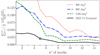 |
Fig. 9. Agreement between w(θ) of a subset of mocks and the mean of w(θ) for all mocks as a function of the number of mocks used for the selection. The dotted red line stands for mocks of 300 deg2, while the dot-dashed blue line represents mocks of 900 deg2 and the dashed green one corresponds to mocks of 1500 deg2 The solid black line stands for mocks of 4108.47 deg2 with the mask of DES Y3 BAO data. The black open circle denotes the selection of the number of mocks and area used for the calibration in this analysis. The number 15 on the y-axis corresponds to the number of clustering measurements averaged (three angular apertures times five redshift bins). |
Once we have determined how many mocks and which area we will use for the calibration, we need to start sampling the parameter space to determine the best-fit parameters. The main idea is to sample a given hypercube in the parameter space. In each point we generate five mocks using the DES Y3 BAO mask, measure w(θ), and compute the value of the χ2 of the measured w(θ) in the mocks to the real measurements:
 (5)
(5)
We note that C, which enters into the χ2, is the standard covariance matrix of the 1952 mocks and takes into account the correlations between the different tomographic bins. To obtain C we calculated w(θ) for the 1952 mocks previously created using the fixed value for the calibration parameters mentioned above.
This approach is not different from a standard Monte Carlo Markov chain. However, it is important to note that each evaluation in a point of the parameter space is extremely expensive in computational time since it implies generating five DES Y3-like mocks and measuring w(θ) on them. Moreover, we are not interested in the posterior of the calibration parameters M1 and ΔLM, but rather on their best-fit values, since this is the only quantity needed to generate mocks close to the real measurements. A straightforward approach would be to use a simple χ2 minimization algorithm to go directly to the minimum of the χ2 function, but the generation of the mocks contains an intrinsic random component when assigning the position and properties of galaxies. This introduces an important stochastic behavior in our problem and makes unusable the standard minimization algorithms.
In this work, following Tutusaus (in prep.), we have decided to use the differential evolution stochastic minimization algorithm first proposed by Storn & Price (1997). The essential idea of the algorithm is to use a population of candidate solutions. We first initialize the population using a Latin Hypercube sampling; then, iteratively, these candidate solutions are combined to generate a new population and the χ2 is evaluated at each position. In more detail, the distance between two random candidate solutions is used to displace the best candidate solution so far (minimum χ2). If the new candidates are better than the previous ones they are accepted and belong to the new population; otherwise they are discarded and the new population is completed with candidates from the old population. Note that, because of this, the size of the population remains constant. The process ends when the standard deviation of the χ2 values of the population is smaller than a given tolerance times the mean of the χ2 values. The best candidate of the population at the end of the process is the best-fit used to generate the final mocks.
Once the calibration parameters have been determined and the five mocks generated, we can check the agreement between the w(θ) from the mocks and the real measurements to verify how accurate the calibration is. The results are shown in Fig. 10. For each one of the tomographic bins, we represent the data with open black circles and the measurements from the five mocks with red lines. The errors have been obtained as the square root of the diagonal of the covariance matrix. The agreement is well within 1σ for all the bins, giving a goodness of the model  . Degrees of freedom (d.o.f.) equal five corresponds to the number of θ-bins = 15, three apertures times five tomographic bins, minus the ten free parameters, two (M1 and ΔLM) per bin.
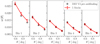 |
Fig. 10. Agreement between the pre-unblinding w(θ) measurements of the data (open black circle) and the output of the calibrated mocks for the five tomographic redshift bins (red lines). The error bars from the mock measurements have been obtained as the square root of the diagonal of the covariance matrix using the 1952 mocks created with the fixed values. |
6. Analysis
In previous sections, we explained the methodology and the procedure used to create 1952 mocks reproducing all the relevant properties of the DES Y3 sample. In this section, we analyze the clustering of these mock catalogs in different spaces. We also include in the analysis a theoretical model prediction for those statistics.
6.1. Theoretical model
The theoretical template is computed using the redshift-space power spectrum
![Mathematical equation: $$ \begin{aligned} P(k, \mu )&= ( 1 + \beta \mu ^2 )^2 b^2 \big \{ [ P_{\rm lin}(k) - P_{\rm sm}(k) ] D_{\rm BAO} + P_{\rm sm}(k) \big \} , \end{aligned} $$](/articles/aa/full_html/2021/12/aa41744-21/aa41744-21-eq15.gif) (6)
(6)
where μ is the dot product between  and the line-of-sight direction, b is the linear bias, and β = f/b with f being the linear growth rate. The power spectrum is built using the linear power spectrum Plin(k) and the linear no-wiggle power spectrum Psm12. The nonlinear damping of the BAO feature is modeled by
![Mathematical equation: $$ \begin{aligned} D_{\rm BAO} (k,\mu ) = \exp \{ - k^2 [ \mu ^2 \Sigma ^2_{\parallel } + (1-\mu ^2) \Sigma ^2_{\perp } + f \mu ^2 (\mu ^2 -1 ) \delta \Sigma ^2 ]\} , \end{aligned} $$](/articles/aa/full_html/2021/12/aa41744-21/aa41744-21-eq17.gif) (7)
(7)
with Σ∥ = (1 +f)Σ⊥. The damping scales Σ⊥ and δΣ are computed following Baldauf et al. (2015). In MICE cosmology, Σ⊥ = 5.80 Mpc h−1 and δΣ = 3.18 Mpc h−1 at redshift 0 and they are scaled to higher redshift by the growth factor. See DES Collaboration (2021) for more details about the procedure to obtain these quantities. Once provided with P(k, μ), we computed the anisotropic redshift-space correlation function ξ(s, μ) through a Fourier transform (see Chan, in prep.). The angular correlation function is obtained after projecting ξ weighted by the redshift distribution n(z) (normalized to 1),
 (8)
(8)
The harmonic power spectrum template Cℓ is derived from w by a Legendre transform
 (9)
(9)
where ℒℓ is the Legendre polynomial. For more details on the modeling, see the main DES Y3 BAO paper (DES Collaboration 2021).
6.2. Angular correlation function: w(θ)
Around ten thousand ACF must be calculated for the mocks (1952 mocks times five bins). For this reason, we resort to a code that allows the calculation using pixels, reducing the computational time. It is important to point out that since we only use angular apertures greater than one degree for fitting, any effect from the pixelization should be negligible. We use the public code CUTE (Alonso 2012). CUTE supports the Landy & Szalay estimator (Landy & Szalay 1993):
 (10)
(10)
where DD, DR and RR represent the total number of Data-Data, Data-Random and Random-Random pairs separated by an angular θ projected distance, respectively. In this case, Data correspond to galaxies in the mocks while Randoms are created by sampling the same volume with random points. The total number of randoms is 20 times the average number of galaxies in the mocks. The same random catalog is used to calculate the clustering for all 1952 mocks. The chosen pixel resolution is npix-shp = 4096 which yields pixels with an angular θ resolution of 2.1 arcmin.
Figure 11 shows the result of the angular two-point correlation function of 1952 mocks for the 5 tomographic bins. It can be noticed that the difference between the pre-unblinding values used for calibration (open black circles) and the averaged ACF for the mocks (solid red lines) differs from what was obtained on Sect. 5 during the calibration procedure (see Fig. 10). However, these small differences are expected given the degree of representativeness when using only five mocks for the calibration (0.25% of the total number of mocks). It is important to keep in mind that the number of five mocks has been determined with a fixed calibration. Therefore, combining the error introduced by these fixed parameters and the allowed 2% accuracy, we can expect the final accuracy with the best-fit calibration and all mocks to be slightly above 2%. To be more precise, this number has increased from 2 to 3.1%. However, within the corresponding uncertainties, the agreement is still within 1σ for the five tomographic bins, giving a global  . The increase in the
  may be due either to the low representativeness of the five mocks used for the calibration or the presence of a strong anti-correlation among the data points. Nevertheless, when we quantify the goodness of the fit between the mocks to the data, using all θ bins in Fig. 11, we find remarkable good values
 ![Mathematical equation: $ \chi_{m-d}^2/{\rm d.o.f.} = [51.2,22.5,24.1,31.6,24.62]/22 $](/articles/aa/full_html/2021/12/aa41744-21/aa41744-21-eq23.gif) . Only the first tomographic bin is away from having a
. Only the first tomographic bin is away from having a  and a bit less is the fourth bin. In conclusion, such accuracy is enough for our purposes and we do not consider rerunning the pipeline with more mocks in each point of the calibration. In more detail, only the first bin shows one pre-unblinding data point out of 1σ from the mocks. In this case, the mean w(θ) of the mock has changed ∼4% from the value found during the calibration. Although this value is double of 2% what was foreseen in the calibration (see Fig. 9), the global change is within the expectation. Blue curves in Fig. 11 denotes the theoretical prediction described in Sect. 6.1, and it is clear from the figure that modeled w(θ) agree almost perfectly with the measurements on the mocks. Finally, solid black lines with error bars correspond to the final post-unblinding measurements of the data (using a brute force configuration of CUTE).
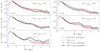 |
Fig. 11. Angular two-point correlation function for each tomographic bin. Red lines correspond to the average over all the mocks and shaded light-red bands correspond to the standard deviation. Dashed blue lines indicate the theoretical prediction described on Sect. 6.1 and black points correspond to the pre-unblinding data values used in the calibration showed on Sect. 5. Finally, solid black lines with error bars represent the final post-unblinding measurement of the data. |
6.3. Projected Clustering: ξw(s⊥)
In photometric surveys, most of the radial BAO information is lost due to redshift uncertainties. Additionally, the photo-z uncertainty causes the BAO scale in the 3D correlation function, ξ(s), to deviate from its true position. However, Ross et al. (2017) demonstrated that when the correlation function is plotted against the transverse scale  , the BAO peak appears where s⊥ equals to the true sound horizon scale. Thus, (angular) BAO information can still be retrieved via the 3D correlation analysis.
Following the methodology from Ross et al. (2017) and also described in DES Collaboration (2021), we show in Fig. 12 the 3D wedge correlation function ξw(s⊥) measured from the mocks (due to computational expenses, only 120 mocks are used) and data. The results are also obtained from CUTE using Eq. (10), by replacing w(θ) with ξ(s⊥, s∥), and then integrating over s∥ for the scales with μ < 0.8. As a comparison, we have also plotted the corresponding theory prediction. While Ross et al. (2017) assumes Gaussian photo-z distribution, the prediction makes use of the photo-z distribution from the mocks, resulting in better agreement with the numerical measurements. Further details of the comparison between the mock results and the theory will be presented in Chan (in prep.). We find a good agreement for the 3D clustering of data, mocks and theory.
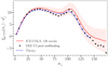 |
Fig. 12. 3D wedge correlation function for μ range [0, 0.8]. With the same color code as previous figures, solid red line corresponds to ICE-COLA mocks and shaded light-red band to its standard deviation. Post-unblinding measurement of data is shown with black points and the theory with a dashed blue line. |
6.4. Angular power spectrum: Cℓ
We also measured the clustering signal in the Fourier conjugate space of angular distances on the sphere, the so-called harmonic space, by estimating the angular power spectra of galaxy number counts, Cℓ. Although constructed from the same underlying field, the angular power spectrum and the correlation function present different advantages and downsides. Most notably, the correlation function is relatively straightforward to estimate in the presence of an angular survey mask. Still, its estimates are largely correlated. On the other hand, the power spectrum requires a deconvolution of the angular mask, but the correlation between scales reduces. Taking these pros and cons into account, it is clearly desirable to have complementary information from both statistics. See Giannantonio et al. (2016) for the first implementation of these complementary estimators in the context of DES Y1 data analyses.
We begin by estimating pixelized galaxy overdensity maps,  , for the ICE-COLA mocks, where
  is the pixel position in the sphere,
  the pixelized galaxy number counts and
  the mean number of galaxies per pixel. We then used the “Pseudo-Cℓ” method (Hivon et al. 2002) to estimate the angular power spectra. The Pseudo-Cℓ method deconvolves the incomplete sky coverage mode mixing effect on a set of band power bins using analytical methods and has the advantage of being less computationally expensive, reaching equivalent error estimates than optimal quadratic estimators. Also, Pseudo-Cℓ estimators are effectively “unbiased” concerning maximum likelihood estimators. In particular, we use the implementation of the NaMASTER code13 (Alonso et al. 2019).
The discrete nature of galaxy number counts introduces a shot-noise contribution to the estimated galaxy overdensity maps and, consequently, a bias to the estimated Cℓ. We account for this “noise bias” analytically, following Alonso et al. (2019) and Nicola et al. (2020) by subtracting this Poissonian noise from our power spectrum. For each ICE-COLA mock, we consider the partial sky coverage introduced by its associated mask, as shown in Fig. 8. To optimize the BAO feature detection, we bin the power spectra in bands of Δℓ = 20 from a minimum multipole ℓmin = 10 up to a maximum multipole of 1 000.
Figure 13 shows the mean and standard deviation of the estimated angular power spectra of the 1952 ICE-COLA mocks for the five tomographic bins (solid red lines) together with the theory prediction (dashed blue lines). Black points correspond to the post-unblinding measurements of the data.
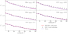 |
Fig. 13. Measured angular power spectra for the tomographic redshift bins considered. Red lines correspond to the average over all the mocks and black points represent the post-unblinding measurements of the data. The theoretical prediction is shown with dashed blue lines. |
7. Effect of replications
Without taking into account the tails on redshift distribution for the tomographic bins on the edges ([0.6 − 0.7] and [1.0 − 1.1]), the maximum comoving line-of-sight distance that can be found among galaxies on the mocks is ∼1000 Mpc h−1. Even if we consider the tails, the distance is lower than the box of the simulation, 1536 Mpc h−1. In other words, no halo of ICE-COLA simulations is used more than one time along any give line-of-sight. But this problem does occur for different lines-of-sight. The area of the survey is very wide implying that for higher redshift several numbers of simulated boxes are used to equal the volume of the BAO Y3 sample. Inevitably this implies the use of the same halo structures on each mock. These repeated halos leave at different times but originate from the same initial structure they will obviously correlate, to leading order overdensities just grow linearly.
Table 2 shows the upper limit for the percentage of replicated “halos” that can be found among bins. To obtain these values, we randomly sampled a box with particles and then created the light cone by replicating this box. These numbers are representative of all the repeated “halos” in a light cone and not only those used to make up the DES Y3 sample, which are a few percent of the total. This fact, together with the selection efficiency, makes that the values are shown on Table 2 stand for a very conservative bound. However, these numbers refer to the replications present in a single mock but each light cone is used to create four mocks (see Fig. 8). This inevitably will introduce replications among different mocks created with the same light cone in addition to those among the bins of a single mock. Numbers in parentheses in Table 2 correspond to the percentage of repeated random particles among the four mocks made from one light cone. For example, the pair of bins (1,3) has on average (mean among the four mocks) 11.9% repeated random particles. This number increase to 30.2% when considering the four mocks. The difference between the 11.9 and the 30.2% come from the particles which are not repeated in one mock but do in others.
Percentage of replications among tomographic bins.
The main impact of this replication problem becomes noticeable when the cross-covariance matrix is analyzed. The repeated structures in different bins introduce a spurious correlation among measured w(θ) of tomographic bins. This effect is shown in Fig. 14 wherein the top panel we compare the covariance matrix of the ICE-COLA mocks (lower diagonal) with the covariance matrix computed using COSMOLIKE halo model (Krause & Eifler 2017; Fang et al. 2020, upper diagonal). From the former, the high degree of correlation between bins that are not adjacent is visible. This strong correlation can be seen clearly in the bottom panel of Fig. 14 where we show one column of the covariance matrix corresponding to an aperture of θ = 2.7 deg for COSMOLIKE (solid black line) and ICE-COLA (dashed blue line). For simplicity, we are using in this plot a Δθ = 0.2.
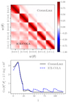 |
Fig. 14. Covariance matrix of the angular correlation function. Top: comparison of the correlation matrix obtained from COSMOLIKE halo model (upper diagonal) and from ICE-COLA mocks (lower diagonal). Bottom: columm of the covariance matrix Cov[ |


8. Conclusions
The performance of well-validated mocks for DES Y3 BAO analysis is crucial for obtaining robust scientific results. The analysis of the data collected by the Dark Energy Survey during the first 3 years of the project poses a great scientific challenge in the development of the required mocks. We have created a significant number of mocks, 1952, adequate for statistical analysis of galaxy clustering. The mocks have been built by populating the halo catalogs of 488 ICE-COLA fast simulations. This task is made up of many steps that make up our pipeline, those are:
-
HALO CATALOGS – Run 488 ICE-COLA simulations with different initial conditions. Create light cones halo catalogs on-the-fly by replicating simulated boxes.
-
GALAXY CATALOGS
-
HOD: Populate halos with one central galaxy and Nsat satellite galaxies following a Poisson distribution, setting the first free parameter per tomographic bin, M1.
-
HAM: Assign a pseudo-luminosity lp to galaxies, setting the second free parameter per tomographic bin, ΔLM.
-
Model photometric redshifts using a highly accurate method which follows a 2D probability distribution relating photometric and spectroscopic redshifts of VIPERS data.
-
Apply four DES Y3 BAO mask over each full-sky light cone and quadrupling the total number of galaxy mocks compared to halo catalogs.
-
-
CALIBRATION – Set an automatic calibration procedure using a differential evolution stochastic minimization algorithm to find the best values for the ten free parameters. This step is a loop of step (ii).
-
FINAL GALAXY CATALOGS – Repeat step (ii) with the final set of parameters.
The automatic calibration and the photometric redshift assignment procedure are key to obtaining final mocks that reproduce with high accuracy the principal properties of the data: (1) observed volume, (2) abundance of galaxies, redshift distribution, redshift uncertainty, and (3) clustering as a function of redshift. Firstly (1), the replications of the simulated box allowed us to achieve the observational volume of the DES Y3 sample. However, the use of even bigger simulations would be beneficial, to avoid the repetition of structures and therefore the introduction of spurious cross-correlations and cross-covariance among not adjacent bins. This should be considered when designing mocks for the calculation of the covariance matrix in future surveys. Secondly (2), the use of overlapping galaxies between DES Y3 and VIPERS gave rise to a very realistic photo-z assignment. In these mocks, the abundance of galaxies, n(zphoto), the redshift distribution N(zspec) and their uncertainties  , W68 and σ68 are in excellent agreement with VIPERS data, showing discrepancies lower than one per cent. Finally (3), the clustering measured in this set of mocks shows an excellent agreement with the pre-unblinding data used for calibration. The uncertainty on the calibration procedure resulted in a goodness of the model
  while for the final mocks this value increased a bit up to 16.72/5.
DES Collaboration (2021) presents the best fit and uncertainty for the angular scale of the BAO angular distance measurement DA using the Y3 Dark Energy Survey data release. The mocks presented in this work have been a crucial tool in the procedure of obtaining these results. ICE-COLA mocks have been used to run robustness tests and optimize the methodology. Finally, it is important to remark that the pipeline that created this set of mocks should work perfectly for any future surveys which need realistic mocks for galaxy clustering analysis.
DES Data Management in National Center for Supercomputing Applications (NCSA, Morganson et al. 2018).
More information is available at http://maia.ice.cat/mice/
Defined by following the 1D Gaussian smoothing in log-space described in Appendix A of Vlah et al. (2016).
Acknowledgments
Funding for the DES Projects has been provided by the U.S. Department of Energy, the U.S. National Science Foundation, the Ministry of Science and Education of Spain, the Science and Technology Facilities Council of the United Kingdom, the Higher Education Funding Council for England, the National Center for Supercomputing Applications at the University of Illinois at Urbana-Champaign, the Kavli Institute of Cosmological Physics at the University of Chicago, the Center for Cosmology and Astro-Particle Physics at the Ohio State University, the Mitchell Institute for Fundamental Physics and Astronomy at Texas A&M University, Financiadora de Estudos e Projetos, Fundação Carlos Chagas Filho de Amparo à Pesquisa do Estado do Rio de Janeiro, Conselho Nacional de Desenvolvimento Científico e Tecnológico and the Ministério da Ciência, Tecnologia e Inovação, the Deutsche Forschungsgemeinschaft and the Collaborating Institutions in the Dark Energy Survey. The Collaborating Institutions are Argonne National Laboratory, the University of California at Santa Cruz, the University of Cambridge, Centro de Investigaciones Energéticas, Medioambientales y Tecnológicas-Madrid, the University of Chicago, University College London, the DES-Brazil Consortium, the University of Edinburgh, the Eidgenössische Technische Hochschule (ETH) Zürich, Fermi National Accelerator Laboratory, the University of Illinois at Urbana-Champaign, the Institut de Ciències de l’Espai (IEEC/CSIC), the Institut de Física d’Altes Energies, Lawrence Berkeley National Laboratory, the Ludwig-Maximilians Universität München and the associated Excellence Cluster Universe, the University of Michigan, NSF’s NOIRLab, the University of Nottingham, The Ohio State University, the University of Pennsylvania, the University of Portsmouth, SLAC National Accelerator Laboratory, Stanford University, the University of Sussex, Texas A&M University, and the OzDES Membership Consortium. Based in part on observations at Cerro Tololo Inter-American Observatory at NSF’s NOIRLab (NOIRLab Prop. ID 2012B-0001; PI: J. Frieman), which is managed by the Association of Universities for Research in Astronomy (AURA) under a cooperative agreement with the National Science Foundation. The DES data management system is supported by the National Science Foundation under Grant Numbers AST-1138766 and AST-1 536171. The DES participants from Spanish institutions are partially supported by MICINN under grants ESP2017-89838, PGC2018-094773, PGC2018-102021, SEV-2016-0588, SEV-2016-0597, and MDM-2015-0509, some of which include ERDF funds from the European Union. IFAE is partially funded by the CERCA program of the Generalitat de Catalunya. Research leading to these results has received funding from the European Research Council under the European Union’s Seventh Framework Program (FP7/2007-2013) including ERC grant agreements 240672, 291329, and 306478. We acknowledge support from the Brazilian Instituto Nacional de Ciência e Tecnologia (INCT) do e-Universo (CNPq grant 465376/2014-2). This manuscript has been authored by Fermi Research Alliance, LLC under Contract No. DE-AC02-07CH11359 with the U.S. Department of Energy, Office of Science, Office of High Energy Physics. This manuscript has been authored by Fermi Research Alliance, LLC under Contract No. DE-AC02-07CH11359 with the U.S. Department of Energy, Office of Science, Office of High Energy Physics. The simulation production and storage, as well as the processing and analysis tools have been developed, implemented and operated in collaboration with the Port d’Informació Científica (PIC). SA was supported by the MICUES project, funded by the EU’s H2020 MSCA grant agreement no. 713366 (InterTalentum UAM). ACR acknowledges financial support from the Spanish Ministry of Science, Innovation and Universities (MICIU) under grant AYA2017-84061-P, co-financed by FEDER (European Regional Development Funds) and by the Spanish Space Research Program “Participation in the NISP instrument and preparation for the science of EUCLID" (ESP2017-84272-C2-1-R). This project has received funding from the European Union’s Horizon 2020 Research and Innovation Programme under the Marie Skłodowska-Curie grant agreement No. 734374.
References
- Alam, S., Aubert, M., Avila, S., et al. 2021, Phys. Rev. D, 103, 083533 [NASA ADS] [CrossRef] [Google Scholar]
- Alonso, D. 2012, ArXiv e-prints [arXiv:1210.1833] [Google Scholar]
- Alonso, D., Sanchez, J., Slosar, A., & LSST Dark Energy Science Collaboration 2019, MNRAS, 484, 4127 [NASA ADS] [CrossRef] [Google Scholar]
- Avila, S., Murray, S. G., Knebe, A., et al. 2015, MNRAS, 450, 1856 [NASA ADS] [CrossRef] [Google Scholar]
- Avila, S., Crocce, M., Ross, A. J., et al. 2018, MNRAS, 479, 94 [NASA ADS] [CrossRef] [Google Scholar]
- Baldauf, T., Mirbabayi, M., Simonović, M., & Zaldarriaga, M. 2015, Phys. Rev. D, 92, 043514 [NASA ADS] [CrossRef] [Google Scholar]
- Benson, A. J., Cole, S., Frenk, C. S., Baugh, C. M., & Lacey, C. G. 2000, MNRAS, 311, 793 [NASA ADS] [CrossRef] [Google Scholar]
- Beutler, F., Blake, C., Colless, M., et al. 2011, MNRAS, 416, 3017 [NASA ADS] [CrossRef] [Google Scholar]
- Blot, L., Corasaniti, P.-S., Rasera, Y., & Agarwal, S. 2021, MNRAS, 500, 2532 [Google Scholar]
- Camacho, H., Kokron, N., Andrade-Oliveira, F., et al. 2019, MNRAS, 487, 3870 [NASA ADS] [CrossRef] [Google Scholar]
- Carnero Rosell, A. C., Rodriguez-Monroy, M., Crocce, M., et al. 2022, MNRAS, 509, 778 [Google Scholar]
- Carretero, J., Castander, F. J., Gaztañaga, E., Crocce, M., & Fosalba, P. 2015, MNRAS, 447, 646 [NASA ADS] [CrossRef] [Google Scholar]
- Chan, K. C., Crocce, M., Ross, A. J., et al. 2018, MNRAS, 480, 3031 [NASA ADS] [CrossRef] [Google Scholar]
- Chuang, C.-H., Kitaura, F.-S., Prada, F., Zhao, C., & Yepes, G. 2015a, MNRAS, 446, 2621 [NASA ADS] [CrossRef] [Google Scholar]
- Chuang, C.-H., Zhao, C., Prada, F., et al. 2015b, MNRAS, 452, 686 [CrossRef] [Google Scholar]
- Coles, P., & Jones, B. 1991, MNRAS, 248, 1 [NASA ADS] [CrossRef] [Google Scholar]
- Comparat, J., Jullo, E., Kneib, J.-P., et al. 2013, MNRAS, 433, 1146 [Google Scholar]
- Conroy, C., Wechsler, R. H., & Kravtsov, A. V. 2006, ApJ, 647, 201 [Google Scholar]
- Cooray, A., & Sheth, R. 2002, Phys. Rep., 372, 1 [Google Scholar]
- Crocce, M., Castander, F. J., Gaztañaga, E., Fosalba, P., & Carretero, J. 2015, MNRAS, 453, 1513 [NASA ADS] [CrossRef] [Google Scholar]
- Crocce, M., Ross, A. J., Sevilla-Noarbe, I., et al. 2019, MNRAS, 482, 2807 [NASA ADS] [CrossRef] [Google Scholar]
- DES Collaboration 2019, MNRAS, 483, 4866 [NASA ADS] [CrossRef] [Google Scholar]
- DES Collaboration (Abbott, T. M. C., et al.) 2021, ArXiv e-prints [arXiv:2107.04646] [Google Scholar]
- De Vicente, J., Sánchez, E., & Sevilla-Noarbe, I. 2016, MNRAS, 459, 3078 [NASA ADS] [CrossRef] [Google Scholar]
- Drlica-Wagner, A., Sevilla-Noarbe, I., Rykoff, E. S., et al. 2018, ApJS, 235, 33 [Google Scholar]
- Euclid Collaboration (Desprez, G., et al.) 2020, A&A, 644, A31 [EDP Sciences] [Google Scholar]
- Fang, X., Eifler, T., & Krause, E. 2020, MNRAS, 497, 2699 [NASA ADS] [CrossRef] [Google Scholar]
- Flaugher, B., Diehl, H. T., Honscheid, K., et al. 2015, AJ, 150, 150 [Google Scholar]
- Fosalba, P., Crocce, M., Gaztañaga, E., & Castander, F. J. 2015a, MNRAS, 448, 2987 [NASA ADS] [CrossRef] [Google Scholar]
- Fosalba, P., Gaztañaga, E., Castander, F. J., & Crocce, M. 2015b, MNRAS, 447, 1319 [NASA ADS] [CrossRef] [Google Scholar]
- Giannantonio, T., Fosalba, P., Cawthon, R., et al. 2016, MNRAS, 456, 3213 [Google Scholar]
- Guo, Q., White, S., Li, C., & Boylan-Kolchin, M. 2010, MNRAS, 404, 1111 [NASA ADS] [Google Scholar]
- Guzzo, L., Scodeggio, M., Garilli, B., et al. 2014, A&A, 566, A108 [NASA ADS] [CrossRef] [EDP Sciences] [Google Scholar]
- Hivon, E., Górski, K. M., Netterfield, C. B., et al. 2002, ApJ, 567, 2 [NASA ADS] [CrossRef] [Google Scholar]
- Izard, A., Crocce, M., & Fosalba, P. 2016, MNRAS, 459, 2327 [NASA ADS] [CrossRef] [Google Scholar]
- Izard, A., Fosalba, P., & Crocce, M. 2018, MNRAS, 473, 3051 [NASA ADS] [CrossRef] [Google Scholar]
- Jing, Y. P., Mo, H. J., & Börner, G. 1998, ApJ, 494, 1 [NASA ADS] [CrossRef] [Google Scholar]
- Kitaura, F.-S., Rodríguez-Torres, S., Chuang, C.-H., et al. 2016, MNRAS, 456, 4156 [NASA ADS] [CrossRef] [Google Scholar]
- Koda, J., Blake, C., Beutler, F., Kazin, E., & Marin, F. 2016, MNRAS, 459, 2118 [NASA ADS] [CrossRef] [Google Scholar]
- Komatsu, E., Dunkley, J., Nolta, M. R., et al. 2009, ApJS, 180, 330 [NASA ADS] [CrossRef] [Google Scholar]
- Krause, E., & Eifler, T. 2017, MNRAS, 470, 2100 [NASA ADS] [CrossRef] [Google Scholar]
- Kravtsov, A. V., Berlind, A. A., Wechsler, R. H., et al. 2004, ApJ, 609, 35 [Google Scholar]
- Landy, S. D., & Szalay, A. S. 1993, ApJ, 412, 64 [Google Scholar]
- Lippich, M., Sánchez, A. G., Colavincenzo, M., et al. 2019, MNRAS, 482, 1786 [NASA ADS] [CrossRef] [Google Scholar]
- Manera, M., Scoccimarro, R., Percival, W. J., et al. 2013, MNRAS, 428, 1036 [Google Scholar]
- Morganson, E., Gruendl, R. A., Menanteau, F., et al. 2018, PASP, 130, 074501 [NASA ADS] [CrossRef] [Google Scholar]
- Navarro, J. F., Frenk, C. S., & White, S. D. M. 1996, ApJ, 462, 563 [Google Scholar]
- Nicola, A., Alonso, D., Sánchez, J., et al. 2020, JCAP, 2020, 044 [Google Scholar]
- Peebles, P. J. E., & Yu, J. T. 1970, ApJ, 162, 815 [NASA ADS] [CrossRef] [Google Scholar]
- Percival, W. J., Cole, S., Eisenstein, D. J., et al. 2007, MNRAS, 381, 1053 [Google Scholar]
- Ross, A. J., Banik, N., Avila, S., et al. 2017, MNRAS, 472, 4456 [NASA ADS] [CrossRef] [Google Scholar]
- Scoccimarro, R., & Sheth, R. K. 2002, MNRAS, 329, 629 [NASA ADS] [CrossRef] [Google Scholar]
- Seljak, U. 2000, MNRAS, 318, 203 [Google Scholar]
- Sevilla-Noarbe, I., Bechtol, K., Carrasco Kind, M., et al. 2021, ApJS, 254, 24 [NASA ADS] [CrossRef] [Google Scholar]
- Sheth, R. K., & Diaferio, A. 2001, MNRAS, 322, 901 [Google Scholar]
- Storn, R., & Price, K. V. 1997, J. Glob. Optim., 11, 341 [CrossRef] [Google Scholar]
- Sunyaev, R. A., & Zeldovich, Y. B. 1970, Ap&SS, 7, 3 [NASA ADS] [Google Scholar]
- Tassev, S., Zaldarriaga, M., & Eisenstein, D. J. 2013, JCAP, 2013, 036 [Google Scholar]
- Vlah, Z., Seljak, U., Yat Chu, M., & Feng, Y. 2016, JCAP, 2016, 057 [CrossRef] [Google Scholar]
- Zhao, C., Chuang, C.-H., Bautista, J., et al. 2021, MNRAS, 503, 1149 [CrossRef] [Google Scholar]
All Tables
All Figures
|
Fig. 1. DES Y3 sample footprint, covering 4108.47 deg2 of the southern sky. |
| In the text | |
|
Fig. 2. Top panel: ratio of the Halo Mass Function between MICE and ICE-COLA. Blue for redshift z = 0.5 and red for z = 1. Shaded areas correspond to the standar deviation of the 488 ICE-COLA runs. Bottom panel: ratio between the MICE and the ICE-COLA ACF for a sample of halos with Mhalo > 1.46 × 10¹² M⊙. |
| In the text | |
|
Fig. 3. Evolution of the first HOD free parameter M1. One value for each tomographic bin. Dashed line correspond to the interpolation assumed for all the redshift range. |
| In the text | |
|
Fig. 4. Evolution of the second HOD parameter ΔLM. One value for each tomographic bin. Dashed line corresponds to the interpolation assumed for all redshift range. |
| In the text | |
|
Fig. 5. Photometric redshift distribution of data and mocks. Gray histogram corresponds to DES Y3 sample. Red points represent the average over the 1952 ICE-COLA mocks and error bars denote the maximum and minimum. |
| In the text | |
|
Fig. 6. True redshift zspec distribution in each tomographic bin. Green filled histograms correspond to VIPERS, black lines represent the distribution for Y3 data and red point are the average over the 1952 ICE-COLA mocks, while error bars correspond to the maximum and minimum. Histograms are normalized to have an integral of unity. |
| In the text | |
|
Fig. 7. Basic metrics for the photo-z validation on each tomographic bin. From top to bottom: difference between |
| In the text | |
|
Fig. 8. Configuration of four DES Y3 BAO footprints on a full-sky. Mask are constructed with HEALPix assuming a resolution NSIDE=4096. |
| In the text | |
|
Fig. 9. Agreement between w(θ) of a subset of mocks and the mean of w(θ) for all mocks as a function of the number of mocks used for the selection. The dotted red line stands for mocks of 300 deg2, while the dot-dashed blue line represents mocks of 900 deg2 and the dashed green one corresponds to mocks of 1500 deg2 The solid black line stands for mocks of 4108.47 deg2 with the mask of DES Y3 BAO data. The black open circle denotes the selection of the number of mocks and area used for the calibration in this analysis. The number 15 on the y-axis corresponds to the number of clustering measurements averaged (three angular apertures times five redshift bins). |
| In the text | |
|
Fig. 10. Agreement between the pre-unblinding w(θ) measurements of the data (open black circle) and the output of the calibrated mocks for the five tomographic redshift bins (red lines). The error bars from the mock measurements have been obtained as the square root of the diagonal of the covariance matrix using the 1952 mocks created with the fixed values. |
| In the text | |
|
Fig. 11. Angular two-point correlation function for each tomographic bin. Red lines correspond to the average over all the mocks and shaded light-red bands correspond to the standard deviation. Dashed blue lines indicate the theoretical prediction described on Sect. 6.1 and black points correspond to the pre-unblinding data values used in the calibration showed on Sect. 5. Finally, solid black lines with error bars represent the final post-unblinding measurement of the data. |
| In the text | |
|
Fig. 12. 3D wedge correlation function for μ range [0, 0.8]. With the same color code as previous figures, solid red line corresponds to ICE-COLA mocks and shaded light-red band to its standard deviation. Post-unblinding measurement of data is shown with black points and the theory with a dashed blue line. |
| In the text | |
|
Fig. 13. Measured angular power spectra for the tomographic redshift bins considered. Red lines correspond to the average over all the mocks and black points represent the post-unblinding measurements of the data. The theoretical prediction is shown with dashed blue lines. |
| In the text | |
|
Fig. 14. Covariance matrix of the angular correlation function. Top: comparison of the correlation matrix obtained from COSMOLIKE halo model (upper diagonal) and from ICE-COLA mocks (lower diagonal). Bottom: columm of the covariance matrix Cov[ |
| In the text | |
Current usage metrics show cumulative count of Article Views (full-text article views including HTML views, PDF and ePub downloads, according to the available data) and Abstracts Views on Vision4Press platform.
Data correspond to usage on the plateform after 2015. The current usage metrics is available 48-96 hours after online publication and is updated daily on week days.
Initial download of the metrics may take a while.