| Issue |
A&A
Volume 656, December 2021
Solar Orbiter First Results (Cruise Phase)
|
|
|---|---|---|
| Article Number | A12 | |
| Number of page(s) | 14 | |
| Section | The Sun and the Heliosphere | |
| DOI | https://doi.org/10.1051/0004-6361/202140915 | |
| Published online | 14 December 2021 | |
Solar Orbiter observations of the Kelvin-Helmholtz waves in the solar wind
1
Institut de Recherche en Astrophysique et Planétologie, CNRS, UPS, CNES, 9 Ave. du Colonel Roche, 31028 Toulouse, France
e-mail: This email address is being protected from spambots. You need JavaScript enabled to view it.
2
Laboratoire d’Astrophysique de Bordeaux, Univ. Bordeaux, CNRS, B18N, Allee Georoy Saint-Hilaire, 33615 Pessac, France
3
Department of Mechanics and Aerospace Engineering, Southern University of Science and Technology, Shenzhen 518055, PR China
4
Department of Physics and Astronomy and Bartol Research Institute, University of Delaware, Newark, DE 19716, USA
5
Department of Physics, Faculty of Science, Mahidol University, Bangkok 10400, Thailand
6
Space and Atmospheric Physics, Department of Physics, Blackett Laboratory, Imperial College London, London SW7 2AZ, UK
7
CGAFD, Mathematics, CEMPS, University of Exeter, Exeter, UK
8
LDE3, DAp/AIM, CEA Saclay, 91191 Gif-sur-Yvette, France
9
Department of Space and Climate Physics, University College London, Mullard Space Science Laboratory, Holmbury St. Mary RH5 6NT, UK
Received:
29
March
2021
Accepted:
6
September
2021
Abstract
Context. The Kelvin-HeImholtz (KH) instability is a nonlinear shear-driven instability that develops at the interface between shear flows in plasmas. KH waves have been inferred in various astrophysical plasmas, and have been observed in situ at the magnetospheric boundaries of solar-system planets and through remote sensing at the boundaries of coronal mass ejections.
Aims. KH waves are also expected to develop at flow shear interfaces in the solar wind. While they were hypothesized to play an important role in the mixing of plasmas and in triggering solar wind fluctuations, their direct and unambiguous observation in the solar wind was still lacking.
Methods. We report in situ observations of quasi-periodic magnetic and velocity field variations plausibly associated with KH waves using Solar Orbiter during its cruise phase. They are found in a shear layer in the slow solar wind in the close vicinity of the heliospheric current sheet. An analysis was performed to derive the local configuration of the waves. A 2D magnetohydrodynamics simulation was also set up with approximate empirical values to test the stability of the shear layer. In addition, magnetic spectra of the event were analyzed.
Results. We find that the observed conditions satisfy the KH instability onset criterion from the linear theory analysis, and its development is further confirmed by the simulation. The current sheet geometry analyses are found to be consistent with KH wave development, albeit with some limitations likely owing to the complex 3D nature of the event and solar wind propagation. Additionally, we report observations of an ion jet consistent with magnetic reconnection at a compressed current sheet within the KH wave interval. The KH activity is found to excite magnetic and velocity fluctuations with power law scalings that approximately follow k−5/3 and k−2.8 in the inertial and dissipation ranges, respectively. Finally, we discuss reasons for the lack of in situ KH wave detection in past data.
Conclusions. These observations provide robust evidence of KH wave development in the solar wind. This sheds new light on the process of shear-driven turbulence as mediated by the KH waves with implications for the driving of solar wind fluctuations.
Key words: magnetohydrodynamics (MHD) / instabilities / plasmas / methods: observational / Sun: heliosphere / solar wind
© R. Kieokaew et al. 2021
 Open Access article, published by EDP Sciences, under the terms of the Creative Commons Attribution License (https://creativecommons.org/licenses/by/4.0), which permits unrestricted use, distribution, and reproduction in any medium, provided the original work is properly cited.
1. Introduction
The magnetic Kelvin-Helmholtz (KH) instability is a magnetohydrodynamic (MHD) shear-driven instability frequently observed in solar system plasmas. KH waves can be induced by the KH instability at the surface between two media with different flow velocity and plasma conditions. This shear instability is fundamental and can be found in many flow shear systems throughout the Universe. KH waves that have been most studied in situ are at the Earth’s magnetopause and low-latitude boundary layers where periodic fluctuations of magnetic fields and plasma parameters are observed (e.g., Hones et al. 1981; Fairfield et al. 2000; Hasegawa et al. 2004; Foullon et al. 2008; Eriksson et al. 2016). This is because the Earth’s flank magnetopause is prone to the KH instability onset condition which prefers a weak magnetic field in the direction of the shear flow. Nevertheless, KH waves have also been observed and identified in strong magnetic field environments such as in the solar corona and at the flank of a coronal mass ejection (CME) (e.g., Foullon et al. 2011, 2013; Ofman & Thompson 2011; Möstl et al. 2013) via extreme ultraviolet (EUV) imaging by the Solar Dynamics Observatory (SDO). Variations of the KH instability such as a sinusoidal mode have also been observed in a solar prominence (Hillier & Polito 2018) using the Interface Region Imaging Spectrograph (De Pontieu et al. 2014).
More recently, remote observations above the solar corona using the Heliospheric Imager instrument on board the Solar-Terrestrial Relations Observatory (STEREO/HI1) have revealed a transition in texture of the solar wind from highly anisotropic coronal plasma, or “striae”, to more isotropic, or “flocculated”, solar-wind plasma (DeForest et al. 2016). The transition is found to be consistent with the onset of hydrodynamic and MHD instabilities, leading to the development of turbulence. Qualitatively, this transition is found to occur near the first surface of plasma β = 1, where the β changes from β ≪ 1 near the Sun to β ≈ 1, and the Alfvén critical surface where the solar wind speed reaches the Alfvén speed (V = VA) (Chhiber et al. 2018). Ruffolo et al. (2020) propose that the transition from striae to flocculation of the young solar wind is powered by shear-driven instabilities such as the KH instability, caused by the relative velocities of adjacent coronal magnetic flux tubes. This is supported by compressible MHD numerical simulations in which several features observed by Parker Solar Probe (PSP; Fox et al. 2016) including the magnetic “switchback” signatures near perihelia are reproduced. It is argued that the KH instability can be triggered when the relative velocity between flux tubes is larger than twice the local Alfvén velocity (ΔV > 2VA) when the magnetic field direction is parallel to the direction of the largest velocity shear (Chandrasekhar 1961; Miura & Pritchett 1982). This condition is less stringent if the magnetic field direction does not align with the largest shear direction. An important implication of such a shear-driven instability is that it may lead to shear-driven turbulence just outside the Alfvén critical zone.
In theory, the KH instability may develop at tangential discontinuities (TDs) because there are relative changes in velocity field (V) and magnetic field (B) magnitudes across them while there is no magnetic field component threading through them, which would otherwise stabilize the instability (as for rotational discontinuities). The solar wind is full of TDs (e.g., Burlaga et al. 1977; Knetter et al. 2004; Neugebauer & Giacalone 2010), which separate different plasma regions. TDs are thought of as surfaces that separate adjacent solar wind flux tubes (e.g., Hollweg 1982) that originated from granules, or meso- and super- granules in the Sun’s photosphere (e.g., Roudier & Muller 1986; Axford & McKenzie 1992), with different plasma properties and a composition that are spread out in the heliosphere (e.g., Bruno & Carbone 2005; Borovsky 2008). It was demonstrated theoretically by many authors that TDs can support MHD surface waves (e.g., Hollweg 1982). In particular, TDs could support the KH instability (e.g., Burlaga 1972; Neugebauer et al. 1986). As for the flux tube picture, it was suggested that the KH instability should be induced when adjacent flux tubes move relative to each other with a speed greater than the Alfvén speed (Burlaga 1972). Zaqarashvili et al. (2014) considered the topology of magnetic flux tubes and found that, while the axial B of the flux tubes stabilizes the KH instability, a slight twist in the B, that is when the B does not align with the V, may allow the surface between them with ΔV < VA to become unstable to the KH instability.
Across TDs, an alignment between the change in velocity direction (ΔV) and the change in magnetic field direction (ΔB) are commonly observed (Neugebauer 1985, 2006; Neugebauer et al. 1986; Knetter et al. 2004). This alignment is not expected from the MHD discontinuity theory, unlike at rotational discontinuities where this alignment is expected (Hudson 1970). This alignment of ΔV and ΔB is observed independent of the type of solar wind stream between 1 and 2.2 AU based on IMP 8 and Voyager 2 data (Neugebauer 1985). Based on Helios data, Neugebauer et al. (1986) report that this alignment is also observed as close as 0.3 AU. They further consider the possibility that the KH instability may have developed across TDs and destroyed the random alignment between ΔV and ΔB. Since the number of TDs per unit time decrease with distance from the Sun (e.g., Tsurutani & Smith 1979; Lepping & Behannon 1986), Neugebauer et al. (1986) suggested that the KH instability may have destroyed TDs as the KH instability growth rate becomes larger with decreasing Alfvén speed.
Despite all these postulations, the KH instability has not been observed in situ in the solar wind to our knowledge. Here we report unambiguous in situ KH wave detection using Solar Orbiter observations (SolO; Müller et al. 2020) during its cruise phase. SolO is an ESA mission, launched on February 10, 2020, aimed to study the Sun and inner heliosphere from out-of-ecliptic vantage points. The cruise phase started in June 2020 with the in situ instruments operated nominally after a successful commissioning. SolO was at 0.69 AU during the observations presented here when several periodic fluctuations in plasma parameters are observed.
In this work, we report quasi-periodic magnetic and plasma variations within a shear layer in the slow solar wind consistent with the development of the KH instability, supported by linear theory analysis, numerical simulation, and boundary layer analysis. The paper is organized as follows. First, we present the instrumentation and overview, context, and KH wave observations in Sect. 2. Additionally, we report observations of magnetic reconnection signatures in the KH waves. Then, we focus on the linear theory, boundary layer analyses, numerical simulations, and magnetic spectra of the KH interval in Sect. 3. As this event shows clear evidence of the KH waves in the solar wind, we discuss why it was not observed in past data, as well as its implications for solar wind dynamics in Sect. 4. We summarize our findings and discussion in Sect. 5.
2. Observations
2.1. Instrumentation and overview
We use magnetic field data from the fluxgate vector magnetometer (MAG; Horbury et al. 2020). MAG continuously samples the magnetic field with the rate up to 16 vector/s in the normal mode and up to 128 vector/s in the burst mode with a precision of about 5 pT. We also use particle data from the Proton and Alpha Particle Sensor (PAS) that is part of the Solar Wind Analysis instrument suite (SWA; Owen et al. 2020). PAS provides high-cadence measurements of 3D velocity distribution function of solar wind particles (electrons, protons, alpha particles, and heavy ions). We use the Radial Tangential Normal (RTN) coordinate system throughout this paper unless stated otherwise. In this system, the coordinates are centered at the spacecraft where R is directed radially outward from the Sun to spacecraft, T is longitudinal along the cross product of the Sun’s rotation vector with R, and N completes the right-handed orthogonal set, which points in the latitudinal direction.
On July 23–24, 2020, SolO was at the distance 0.69 AU from the Sun. From July 23 at 12:00 UT to July 24 at 12:00 UT, SolO was moving from the distance r = 1.03 × 10⁸ km (0.68 AU) to r = 1.04 × 10⁸ km (0.70 AU) from the Sun. Figure 1 shows the projected position of SolO onto the equatorial plane with the solar wind Parker spiral (orange lines) (Parker 1958) calculated using a constant solar wind speed of 300 km s−1. This figure is obtained using the 3DView software1 (Génot et al. 2018). The radial speed of SolO was VR = 11.3 km s−1 throughout this interval.
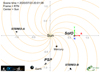 |
Fig. 1. Overview of SolO and other spacecraft positions on 23 July 2020 at 20:01:08 UT projected in a solar equatorial plane in the RTN coordinates centered at SolO. Orange solid lines represent solar wind Parker spirals (Parker 1958) calculated using a constant velocity of 300 km s−1. This figure was obtained using the 3DView software (Génot et al. 2018). |
Figure 2 shows the global context on July 23, 2020 from 18 to 24 UT of the solar observations with the SolO position (blue cross) projected onto the Sun’s surface. This figure is obtained from the Magnetic Connectivity Tool2 (Rouillard et al. 2020). This tool allows us to estimate solar wind source regions as measured by spacecraft in order to connect remote and in situ observations. The tool models the solar corona, based on a magnetostatic reconstruction from magnetograms using the Potential Field Source Surface (PFSS) technique, and the interplanetary magnetic field, based on a Parker spiral orientation. The coronal field is reconstructed based on magnetograms from the ADAPT (Air Force Data Assimilative Photospheric Flux Transport) flux transport model (Arge et al. 2010; Hickmann et al. 2015). The probability of connectivity between coronal sources and in situ observations is then calculated using assumed slow (300 km s−1) and fast (800 km s−1) solar wind streams at the spacecraft position. The tool outputs positions of high connectivity probability for the assumed slow and fast winds with a magnetogram or combined images as a background. Here, the background image is produced by combining images taken by SDO and STEREO-A in EUV at 171 Å, using the AIA and EUVI instruments, respectively. The red and green dots indicate the points at the surface that are most likely to be magnetically connected to SolO, assuming uniform slow and fast wind flows, respectively. The SolO position is estimated to be at the blue cross position. On this image, the SolO position appears at low-latitude (∼0°) and near the heliospheric current sheet (HCS) marked by a red dashed line. In this work, we report SolO observations of the KH waves near an edge of the HCS.
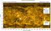 |
Fig. 2. Connectivity map of the observations on July 23, 2020, produced from the Connectivity Tool (Rouillard et al. 2020) to provide a global context. The background is a combined image from remote observation using SDO/AIA and STEREO-A/EUVI 171 Å Carrington maps. The blue cross represents the region of high connectivity probability of SolO to the solar wind source regions. The green and red dots represent zones of the high connectivity probability to the solar wind source regions assuming fast and slow winds, respectively. The heliospheric current sheet (HCS) is marked with a red dashed line. |
2.2. 14-h context
Figure 3 shows SolO observations between 16:00 UT on July 23, 2020 and 6:00 UT on July 24, 2020, covering a 14-h interval. In Fig. 3a, we show the magnetic field components and magnitude. Figure 3b displays the radial component (VR) and Fig. 3c the tangential (VT) and out-of-ecliptic (VN) components of the ion bulk flow velocity. Two main HCS crossings are observed between 22:00 UT on July 23 and 2:00 UT on July 24 in between the purple vertical dotted lines. The HCS is characterized by a large-scale (∼several hours) change in the polarity of the radial magnetic field (BR). Around 18:00 UT on July 23, we mark a meso-scale structure (∼a few hours) between vertical orange dotted lines, characterizing bipolar magnetic fields with a magnetic discontinuity (i.e., current sheet) at the center. At this central current sheet, there is an ion jet clearly seen in VR, VT, and VN components, probably indicating ongoing magnetic reconnection. This structure is known as Magnetic Increase with Central Current Sheet (MICCS) and it has been observed with Parker Solar Probe (Fargette et al. 2021); this signature corresponds to two magnetic flux tubes that become interlinked and with magnetic reconnection at the interface (e.g., Louarn 2004; Kacem et al. 2018; Øieroset et al. 2019; Kieokaew et al. 2020). Although mentioned here for context, this feature is not discussed any more in our study.
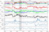 |
Fig. 3. Solar Orbiter observations between 16:00 UT on 23 July 2020 and 6:00 UT on 24 July 2020 showing the context of the Kelvin-Helmholtz instability observation (shaded area). (a) Magnetic fields in the RTN coordinates. (b) Ion bulk velocity VR component. (c) Ion bulk velocity VT and VN components. (d) Ion number density. (e) Alfvén Mach number. (f) Normalized cross-helicity. (g) The angle between δV and B (see text). The heliospheric current sheet (HCS) is observed between 22:00 UT on 23 July 2020 and 2:00 UT on 24 July 2020, marked by purple dotted lines. The Magnetic Increase with Central Current Sheet (MICCS) is observed between 17:35 and 18:08 UT on 23 July 2020, marked by orange dotted lines. |
From 20:45 to 21:30 UT on July 23 in Fig. 3c, we observe a velocity shear of about 30 km s−1 in the VT (green) and about 20 km s−1 in the VN (blue) components. This velocity shear interval features periodic fluctuations in the magnetic fields (Fig. 3a) and the radial velocity (VR; Fig. 3b). The shear layer is also accompanied by changes in the ion number density shown in Fig. 3d. This interval as shaded in gray exhibits quasi-periodic fluctuations that resemble KH waves (with periods of 6−8 min); we show a zoom-in of this interval in the next section.
Figures 3e–g show the Alfvén Mach number (MA), the normalized cross-helicity (σc), and the angle between V change and B (θδV, B), respectively. During the shaded interval, the MA is 12, indicating that the solar wind speed is super-Alfvénic. The σc (Matthaeus & Goldstein 1982; Roberts et al. 1992) is calculated from σc = 2⟨δV ⋅ δb⟩/⟨|δV|2 + |δb|2⟩, where δV = V − ⟨V⟩20 min and δb = b − ⟨b⟩20 min are the velocity field and magnetic field fluctuations from the 20-min running averages of V and  , where μ0 is the vacuum permeability and ρ is the 1-h average proton mass density, respectively. The magnetic field b is measured in Alfvén speed units in km s−1. The sum brackets ⟨…⟩ are taken over 20-min running averages. σc relates to the cross helicity
  and the energy per unit mass
  through the relation σc = 2Hc/E. This quantity measures the Alfvénicity with σc = ±1 indicating Alfvénic fluctuations, where the signs +, − correspond to Alfvénic propagation antiparallel or parallel to the mean field, respectively. During the shaded interval, σc is fluctuating between 0 and 0.5, indicating that the solar wind fluctuations are not strongly Alfvénic. The angle θδV, B is calculated from arccos(δV ⋅ B/(|δV||B|)). The magnetic field in the direction of the velocity jump, that is when θδV, B is near 0° or 180°, has a stabilizing effect on the KH instability due to the magnetic tension exerted in the direction of the shear flow (e.g., Chandrasekhar 1961). For the shaded time period, Fig. 3g shows that the angle between δV and B is spreading from 60° to 120°. The nonalignment of δV and B during this interval indicates the possibility for this shear layer to be unstable to the KH instability with a wave vector perpendicular to B, which minimizes the role of the magnetic tension.
2.3. KH wave observations
Figure 4 shows a zoom-in around the shaded time period in Fig. 3 between 20:45 and 21:30 UT on July 23, 2020. The quasi-periodic fluctuations in several parameters resemble in situ KH waves at the interface between shear flows (e.g., Hasegawa et al. 2004). The magnetic field in Fig. 4a clearly shows repeated, homologous fluctuations in all components. We mark sharp magnetic rotations (1)–(7) with vertical dashed lines. Figure 4b shows VR and Fig. 4c shows VT and VN components of the ion bulk velocity. The velocity shear is clearly seen in the VT component. To mark the shear layer, we define Side 1 at 20:38 UT as the beginning of the shear interval and Side 2 as the end of the shear interval at 21:29 UT, marked by magenta dotted-dashed lines. Sides 1 and 2 are characterized mainly by the tangential velocity VT which reached local minimum and maximum, respectively. The periodic features are also seen in the velocity fields especially for the tangential (VT) component in Fig. 4c in which sudden, sharp transitions colocate with the changes in the magnetic field marked by the vertical dashed lines. To facilitate discussion, we define the magnetic rotations (1)–(7) as “wave edges” that mark sudden changes in both magnetic and velocity fields. Table 1 We notes times of these wave edges and time differences between these edges. These time differences correspond to the period of the waves. The average time difference between wave edges is 7 min 17 s (s) and the standard deviation is 55 s. We analyze the wave edges in detail in Sect. 3.3.
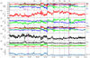 |
Fig. 4. Solar Orbiter observations on 23 July 2020 between 20:10 UT and 21:50 UT. (a) Magnetic field in the RTN coordinates. (b) Ion bulk velocity VR component. (c) Ion bulk velocity VT and VN components. (d) Alfvén speed |VA| and Alfvén velocity components (VA, R, VA, T, VA, N). (e) Ion number density. (f) Plasma pressure Pp, magnetic pressure Pm, and total pressure Ptot. (g) Plasma beta β. The KH waves can be noticed between 20:45 and 21:30 UT. The vertical gray dashed lines (1)–(7) mark the boundary layer crossings corresponding to KH trailing edges. The magenta dashed-dotted lines mark times when the plasma parameters reach asymptotic values on Side 1 (20:38 UT) and Side 2 (21:29 UT) of the shear layer. |
Figure 4d shows Alfvén speed and Alfvén velocity components ( , where ni is the ion number density and mp is the proton mass). The average Alfvén speed in this interval is 26 km s−1. Figure 4e shows the ion number density (nion). Despite some fluctuations, nion gradually changes from 30 cm−1 at Side 1 to 22 cm−1 at Side 2. Figure 4f shows the magnetic (Pm), thermal (Pp), and total pressure (Ptot = Pm + Pp). The total pressure is approximately constant, indicating approximate pressure balance across the shear layer. Figure 4g shows the ion beta (β). The β is changing from β ≈ 2 at Side 1 to β ≈ 1 at Side 2. A strong peak in β of about β ≈ 7 is observed adjacent to wave edge (3). At wave edge (3), there is an ion jet in VN (blue in Fig. 4c) with ΔVN ∼ 11 km s−1 that colocates with the magnetic rotation observed in BN (blue in Fig. 4a). We explain that this ion jet may be produced by magnetic reconnection, in Sect. 2.4.
Table 2 summarizes the values of V, B and nion at Sides 1 and 2. Considering the velocity change across the shear layer, we define ΔV = V2 − V1, where the subscripts 1 and 2 label Sides 1 and 2, respectively. The velocity change is ΔV = (ΔVR, ΔVT, ΔVN) = (20, 30, −11) km s−1, with |ΔV| = 38 km s−1. The ratio of the velocity change across the shear layer to the average Alfvén speed is therefore ΔV/VA = 1.5. The observed shear velocity exceeds the local Alfvén speed but does not satisfy the KH instability criterion (ΔV ≥ 2VA) for the parallel configuration. We note that this condition is obtained in a simplistic configuration of an infinitely thin shear layer embedded in the uniform density and magnetic field and with the magnetic field being exactly along the velocity shear. We further examine the stability of this shear layer using the linear theory in Sect. 3.1 and using an MHD simulation in Sect. 3.2.
2.4. Magnetic reconnection
Figure 5 shows a zoom-in at wave edge (3) in Fig. 4 that contains an ion jet colocated with the change in magnetic field seen in the N component (blue). The current sheet interval at the wave edge is delineated by orange dashed lines between 21:02:00 and 21:02:40 UT. The magnetic field magnitude in Fig. 5a drops at the center of the current sheet to a local minimum of about 2.5 nT. To clearly see the ion jet, we transform the magnetic field into local current sheet “lmn” coordinates using the hybrid Maximum Variance Analysis (MVA) technique (Gosling & Phan 2013). In this coordinate system,  points in the magnetic shear direction (i.e., the reconnecting component),
  points in the direction normal to the shear plane, and
  points in the out-of-plane direction (i.e., the guide-field direction). We transform the magnetic field from the RTN coordinates to lmn coordinates as follows. First, the current sheet normal
  is obtained from the cross-product of the asymptotic 10-s averaged magnetic fields just outside the current sheet interval. Second, the
  component is obtained from
  , where
  is the maximum variance direction obtained from the MVA technique (Sonnerup & Cahill 1967) applied in the current sheet interval. Finally,
  completes the right-handed orthonormal system. We obtain
  = [ − 0.285, 0.245, −0.924],
  = [0.882, 0.44, −0.156], and
  = [0.37, −0.863, −0.343].
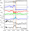 |
Fig. 5. Magnetic reconnection signatures at wave edge (3) in Fig. 4. (a) Magnetic field strength. (b) Magnetic field reconnecting |


The magnetic field rotation is clearly seen in the Bl component in Fig. 5b. Bl rotates from positive to negative during the current sheet interval in colocation with the ion jet seen in the Vl component in Fig. 5e. We note that the velocity data have lower cadence (4 s) than the magnetic field data (1 s), thus the velocity is sampled only at a few points in the vicinity of the current sheet interval. The velocity peak is marked by a gray dashed line. This ion jet has a magnitude of ΔV = 13 km s−1 at 21:02:24 UT. Although there is only one velocity measurement associated with the peak inside the jet, one should note that the operation cycle of the PAS instrument is such that each sample is made over only 1 s every 4 s. The measurement is thus made over a limited time exactly in the center of the current sheet, rather than over 4 s which would have led to significant time aliasing across the current sheet.
The change in Bl correlates with the change in Vl negatively on the inbound side (21:02:00 to 21:02:24 UT) and positively on the outbound side (21:02:24 to 21:02:40 UT). This sequence of correlations is consistent with a jet that is produced by magnetic reconnection. Although we acknowledge that there is only one velocity measurement in the jet, there are additional signatures that are consistent with the interpretation of magnetic reconnection, such as the enhanced ion number density shown in Fig. 5e, consistent with mixing of ions from either side of the current sheet in the reconnection exhaust (Gosling et al. 2005) and the enhanced ion temperature consistent with plasma heating within the reconnection exhaust (Phan et al. 2014) in Fig. 5f.
To more quantitatively assess whether this jet is consistent with reconnection, we consider the Walén relation: ΔVA ∼ ±ΔB/(μ0mpnion)1/2, where + or − is applied for a positive or negative correlation between B and V, respectively, (Hudson 1970; Paschmann et al. 1986) within the exhaust as bounded by dashed orange lines in Fig. 5. The predicted jet velocity is shown as cyan in Fig. 5d. The predicted velocity produces a trend that resembles the observed jet. However, the predicted velocity jet from the Walén relation is estimated to be ΔVA = 33 km s−1. Thus, the observed jet has a velocity that is 40% of the predicted jet velocity. A sub-Alfvénic reconnection jet is not unusual in observations. In the literature, sub-Alfvénic jet speeds are found when the spacecraft crosses the reconnection exhaust near the X-line. The development of secondary instabilities due to high plasma-β was also found to lower the reconnection jet speed (Haggerty et al. 2018). The presence of reconnection within KH waves may imply that it is produced as a consequence of vortex-induced-reconnection (e.g., Nykyri & Otto 2001; Nakamura et al. 2006; Karimabadi et al. 2013; Eriksson et al. 2016), which can be triggered when KH vortices develop and create thin current sheets between them. We further discuss this possibility in the discussion section.
3. Results
3.1. Linear theory analysis
To test whether the observed local conditions in Table 2 satisfy the KH instability onset criterion, we consider the stability of a shear layer derived using the linear theory of Chandrasekhar (1961). The KH instability onset criterion derived for an infinitely thin boundary layer in an incompressible plasma can be written (Hasegawa 1975) as
![Mathematical equation: $$ \begin{aligned} \left[\boldsymbol{k} \cdot (\boldsymbol{V}_1 - \boldsymbol{V}_2) \right]^2 > \frac{n_1 + n_2}{\mu _0 m_{\rm p} n_1 n_2} \left[ (\boldsymbol{k} \cdot \boldsymbol{B}_1)^2 + (\boldsymbol{k} \cdot \boldsymbol{B}_2)^2 \right] \end{aligned} $$](/articles/aa/full_html/2021/12/aa40915-21/aa40915-21-eq19.gif) (1)
(1)
where k is the wave vector, V is the velocity field, B is the magnetic field, and n is the ion number density, with the subscripts 1, 2 representing either side of the shear layer. The phase velocity of the KH mode, associated with the real part of the KH dispersion relation Vph = ω/k, where ω is the wave frequency and k is the wave number, is given as
 (2)
(2)
The growth rate of the KH instability, associated with the imaginary part of the dispersion relation, can be written as
![Mathematical equation: $$ \begin{aligned} \gamma = [ \alpha _1 \alpha _2 [ (\boldsymbol{V}_1 - \boldsymbol{V}_2) \cdot \boldsymbol{k}]^2 - \alpha _1 ({\boldsymbol{V}_{\rm A,1}} \cdot \boldsymbol{k})^2 - \alpha _2 ({\boldsymbol{V}_{\rm A,2}} \cdot \boldsymbol{k})^2 ]^{1/2} \end{aligned} $$](/articles/aa/full_html/2021/12/aa40915-21/aa40915-21-eq21.gif) (3)
(3)
where α1 = n1/(n1 + n2) and α2 = n2/(n1 + n2), and VA, 1, VA, 2 label the Alfvén speeds on either side of the boundary.
To simplify the configuration of the observed shear layer, we transform the velocity field using the application of the MVA technique to the ion bulk velocity from 20:14 to 21:50 UT. The maximum, intermediate, and minimum variance directions are found to be [0.53, 0.79, −0.32],[0.84, −0.53, 0.07], and [0.12, 0.31, 0.95], respectively. The ratios of the maximum to the intermediate eigenvalues (λ1/λ2) and the intermediate to the minimum eigenvalues (λ3/λ2) are 7.7 and 2.0, respectively, indicating reliable estimations (Siscoe & Suey 1972). The maximum variance direction is the direction of the velocity shear direction; it is assigned as X. The intermediate variance direction is the inhomogeneous direction; it is assigned as Y. Finally, the minimum variance direction is the invariant direction; it is assigned as Z. The transformed B and V are shown in Figs. 6a–d. In Fig. 6a, the magnetic flux along the inhomogeneous direction (BY) is not zero on the two sides taken as boundary conditions. Therefore, this velocity shear layer does not have a simple configuration consistent with a TD when one uses Sides 1 and 2 asymptotic values as the boundary conditions of the KH instability (which in reality occurs earlier and closer to the Sun); we further discuss this configuration next. The velocity jump is clearly seen in Fig. 6b with ΔV ≈ 40 km s−1. Figure 6e shows a simplified configuration of this shear layer in the X − Y plane. We note that the VY and VZ are nearly constant and thus not shown in this figure.
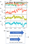 |
Fig. 6. Magnetic and velocity fields in the local shear frame obtained from the application of the MVA to the ion bulk velocity. (a) Magnetic field in the maximum (X), intermediate (Y), and minimum (Z) variance directions and its magnitude. (b–d) Velocity field in the X, Y, and Z directions, respectively. (e) Simplified shear boundary layer configuration obtained from the transformation to the maximum shear frame. |
Figure 6 shows B and V in the frame where the velocity shear ΔV is projected into one direction (X). By the definition of a TD (e.g., Burlaga 1969; Hudson 1970; Lepping & Behannon 1986; Neugebauer et al. 1984; Knetter et al. 2004), there should be no, or at least minimal, magnetic field along the TD normal direction, which is the Y direction (the inhomogeneous direction). In Fig. 6a, BY, 1 = 2 nT and BY, 2 = 4 nT, thus there is a nonzero magnetic flux through the Y direction; therefore, this configuration does not fit the TD description. In fact, for KH waves at a TD, we expect a certain level of quasi-periodic BY fluctuations. This stems from the development of KH vortices that stretch the magnetic field in 3D leading to associated fluctuations in the BX and BY components (here Z is the invariant direction) with ⟨BY⟩ = 0. This type of configuration is typically found for KH development at the Earth’s magnetopause (e.g., Hasegawa et al. 2004; Foullon et al. 2008; Eriksson et al. 2016). The lack of a frame, where the asymptotic magnetic field (taken at meso-scales on each side of the observed waves) along the normal direction is zero, may be due to the complex 3D configuration rather than a simple 1D or 2D as generally assumed for simplicity.
The origin of the lack of such a frame is likely also due to the fact that the KH waves have already evolved and impacted the local and meso-scale geometry so that the properties of the asymptotic magnetic field and flow at the time of observation is not representative of the original current sheet (TD) configuration anymore. In other words, we cannot expect the current asymptotic conditions (Sides 1 and 2) to be strictly relevant for linear theory analysis of the KH instability or for setting up the simulations because the KH instability developed in reality both significantly earlier and closer to the Sun.
Despite the lack of a perfect TD frame, we may test the stability of the shear layer with certain assumptions for the initial configuration. At the initial shear layer, we assume a velocity jump with ΔV = V2 − V1 ≈ (40, 0, 0) km s−1 similar to Fig. 6e. Importantly, we ignore the BY component for the initial shear layer, with the assumption that the original shear layer was a TD and this BY component was later introduced by the KH dynamics. A KH growth rate from this simplified configuration in Fig. 6e with BY, 1 = BY, 2 = 0 can be calculated as follows. Assuming that the wave vector k makes an angle ϕ from the plane containing the shear flow toward the Z-direction such that k = (k cos ϕ, 0, k sin ϕ), Eq. (3) can be written as
![Mathematical equation: $$ \begin{aligned} \left( \frac{\gamma }{k} \right)^2 =&\frac{\rho _1 \rho _2}{(\rho _1 + \rho _2)^2} \left[ \Delta V_x \cos \phi + \Delta V_z \sin \phi \right]^2 \nonumber \\&- \frac{1}{\mu _0 (\rho _1 + \rho _2)} \left[ B_{1,x} \cos \phi + B_{1,z} \sin \phi \right]^2 \nonumber \\&- \frac{1}{\mu _0 (\rho _1 + \rho _2)} \left[ B_{2,x} \cos \phi + B_{2,z} \sin \phi \right]^2 \end{aligned} $$](/articles/aa/full_html/2021/12/aa40915-21/aa40915-21-eq22.gif) (4)
(4)
where ρi = mpni, i = 1, 2. We find positive growth rates for an arbitrary angle ϕ with a maximum growth rate (γ/k) of 16 km s−1. This means that the observed conditions with simplified assumptions at the initial shear layer of this event are unstable to the KH instability. In brief, the linear theory analysis may support the KH instability interpretation.
Assuming that the wave vector k is in the same direction as the flow, we obtain the KH phase velocity from Eq. (2) to be Vph = 152 km s−1. Since the average wave period from Table 1 is found to be 437 ± 55 s (7.3 ± 0.9 min), the KH wavelength is estimated to be λKH = 66 400 ± 8400 km or 0.10 ± 0.01 solar radii. The linear theory analysis of a finite-thickness shear layer by Miura & Pritchett (1982) predicts that the fastest growing mode occurs for kL ∼ 0.5 − 1.0, where L is the initial shear layer thickness. Using k = 2π/λ, the fastest growing mode should have the wavelength of 2πL − 4πL. Using our estimated λKH, we estimate the initial shear layer thickness to be L ≈ 5300 − 10 500 km. We note that this estimate ignores any vortex merging or potential influence of pre-existing turbulence that could influence the size of the vortices that are observed.
3.2. KH simulation
To further test whether the observed conditions would support the KH instability, we performed a numerical simulation using SolO observations for Side 1 and Side 2 as boundary conditions. We exploit a numerical simulation that solves compressible MHD equations via a hybrid compact-weighted essentially non-oscillatory (WENO) scheme (Yang et al. 2016a). This hybrid scheme couples a sixth-order compact finite difference scheme for smooth regions and a fifth-order WENO scheme in shock regions, suitable for capturing strong discontinuities in MHD systems. The time stepping is performed by the third-order Runge-Kutta scheme. This code has been used to study compressible MHD turbulence (Yang et al. 2016b, 2017) and shear-driven turbulence by the KH instability near the Sun (Ruffolo et al. 2020).
To simulate our event, we consider the initial shear layer in Fig. 6e with the simplified configuration, considered in Sect. 3.1. Moreover, we consider the local KH instability frame that travels with the KH phase speed at Vph ≈ 150 km s−1. In this frame, the speeds on Sides 1 and 2 are UX, 1 = −15 km s−1 and UX, 2 = 25 km s−1, respectively. Since the magnetic field perpendicular to the shear flow does not impact the KH growth (Chandrasekhar 1961), we only include magnetic field in the shear flow direction (BX). The ion number density values on Sides 1 and 2 are n1 = 30 cm−3 and n2 = 22 cm−3, respectively. The ion temperature values on Sides 1 and 2 are set to T1 = 1.32 eV and T2 = 3.63 eV, respectively. The ion β is set to 1. The magnetosonic Mach number across the shear layer is ΔU/cs, 1 = 2.75, where ΔU = 40 km s−1 and cs, 1 is the sound speed on Side 1. The Alfvén Mach number is ΔU/VA, 1 = 2.52, where VA, 1 is the Alfvén speed on Side 1.
The numerical simulation is performed using a Lx × Ly = 8π × 4π domain with nx × ny = 1024 × 512 resolution with periodic boundary conditions in the X-direction. For simplicity, equal viscosity and resistivity μ = η are used, i.e., the magnetic Prandtl number is set to unity. We solve the dimensionless form of the MHD equations by introducing several reference scales. The normalizations are U0 = 100 km s−1, n0 = 30 cm−3, B0 = 25 nT, and T0 = 66 eV. The simulation is 2D as we ignore the invariant direction and only impose the magnetic field in the direction of the shear flow.
We set up double shear layers in the simulation domain similar to those of Ruffolo et al. (2020). The velocity and magnetic profiles are only set in the X-direction and both are colocated. The velocity profile is given by
![Mathematical equation: $$ \begin{aligned} u_x = U_\alpha \left[ 1 - \tanh \left( \frac{{ y} - L_{ y} / 4}{d} \right) + \tanh \left( \frac{{ y} - 3L_{ y} / 4}{d} \right) \right] + U_\beta , \end{aligned} $$](/articles/aa/full_html/2021/12/aa40915-21/aa40915-21-eq23.gif) (5)
(5)
where  ,
,  , U1 = −0.15U0, U2 = 0.25U0, and d = 0.003Ly is the half thickness of the shear layer. The magnetic profile is given in a similar way as
![Mathematical equation: $$ \begin{aligned} B_x = B_\alpha \left[ 1 - \tanh \left( \frac{{ y} - L_{ y} / 4}{d} \right) + \tanh \left( \frac{{ y} - 3L_{ y} / 4}{d} \right) \right] + B_\beta , \end{aligned} $$](/articles/aa/full_html/2021/12/aa40915-21/aa40915-21-eq26.gif) (6)
(6)
where  ,
,  , B1 = 0.16B0, and B2 = 0.0. The density is set with ρ1 = ρ0 and ρ2 = 0.73ρ0 in normalized units. The initial temperature profile is set such that the total (magnetic plus thermal) pressure is balanced across the shear layer, where T1 = 0.02T0 and T2 = 0.055T0. Finally, the background shear is initially perturbed by adding a small compressive velocity field in the Y-direction in the form
![Mathematical equation: $$ \begin{aligned} \mathrm{d} u_{ y} = \delta u_0 \left[ e^{\left( \frac{{ y} - L_{ y}/4}{4d} \right)^2} - e^{- \left( \frac{{ y} - 3L_{ y}/4}{4d} \right)^2} \right] \mathrm{ran}(x) \nonumber \end{aligned} $$](/articles/aa/full_html/2021/12/aa40915-21/aa40915-21-eq29.gif)
where δu0 = 0.008(U2 − U1) (i.e., less than 10% of the shear flow magnitude) and ran(x) represents a random number generator in the range [−0.5, 0.5] at each grid value.
Figure 7 shows a snapshot of the simulation at ∼13 large-eddy turnover time for one of the shear layers (the two shear layer develop similar KH instability structures). The color represents the flow vorticity (ω) in the out-of-plane direction. The KH waves are seen to develop in the simulation. They quickly reach the nonlinear stage where rolled-up KH vortices clearly form (from ∼6 large-eddy turnover times onward) with visible vortex merging. This confirms that the solar wind observations by SolO are consistent with the KH instability growth. In the lower part of the simulation (Side 1), there are features seen as stripes in vorticity. These features are shocks that are produced by the supersonic flow on Side 1 (Mach number ∼3) as the speed difference between the recirculating vortex and the nearby passing flow exceeds the sound speed (e.g., Landau & Lifshitz 1987). Shocks created by vortices have been observed in an experimental study of hydrodynamics shear in supersonic regimes (Papamoschou & Roshko 1988) and in MHD simulations of KH instability in super-magnetosonic regimes (Miura 1990; Palermo et al. 2011a,b; Henri et al. 2012). This vortex-induced shock formation is found when the flow surrounding vortices is faster than the vortex speed, characterized by the convective Mach or the vortex Mach number ≳1 (Palermo et al. 2011a,b). Future work ought to determine whether such features are sometimes observed in spacecraft data. For the present work, the key point merely remains that the KH instability does develop for the modeled conditions.
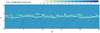 |
Fig. 7. Snapshot of the numerical simulation of the KH instability using empirical values of the SolO event from Side 1 and Side 2 with the initial TD assumption. The color-scale represents values of the out-of-plane flow vorticity (ω). The KH instability quickly reaches the nonlinear stage where rolled-up KH vortices form and coalesce. The stripes in vorticity in the lower part of the simulation are shocks (known as vortex-induced shocks) produced by the supersonic flow as the Mach number on this side is ∼3 (see text). |
3.3. Boundary layer analysis
To understand local configurations of the KH waves, we characterize orientations of the observed wave edges in the RTN coordinates. In Fig. 4, the magnetic rotations are clearly defined for wave edges (2), (3), and (4). Figure 8 shows B and V and their fluctuations from the average values between 20:35 and 21:20 UT with time progressing from right to left. Here, Side 1 (20:38 UT) is to the right and the Side 2 (21:29 UT) is to the left. This reversed time-domain plot is roughly equivalent to a translation in the spatial domain where the waves propagate from left to right relative to SolO, which is relatively static compared to the wave motion. Wave edges (2), (3), and (4) defined by clear rotations of B in Fig. 8a and V in Figs. 8d and e, are marked by cyan vertical dashed lines. We define these sharp discontinuities as the “outbound crossings” from a slow to a faster speed stream. Smaller magnetic field rotations are also visible between these outbound crossings. We mark these smaller rotations as (2′), (3′), and (4′) with magenta vertical dashed lines in Fig. 8. These edges show reverse transitions compared to the outbound crossings in BR (red) and BN (blue) components. We define these smaller transitions as “inbound crossings”. At one of the waveforms, between (2) and (3), the velocity component VR in Fig. 8d shows a turning of the flow direction as circled in blue. This flow deflection pattern corresponds to a vortex-like structure, i.e., a high vorticity region, that is consistent with a perturbation by a rolled-up KH vortex (e.g., Hasegawa et al. 2004; Fairfield et al. 2007; Kieokaew 2019). This indicates that these KH waves may be in a nonlinear stage of development.
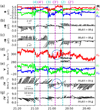 |
Fig. 8. Magnetic and velocity fields with their perturbations from the average shown with time progresses from right to left. Inbound and outbound crossings are marked with purple and cyan vertical dashed lines, respectively. (a) Magnetic fields. (b,c) Magnetic field fluctuations from the averages in the R − T and R − N planes, respectively. (d) Ion bulk velocity VR component. (e) Ion bulk velocity VT and VN components. (f,g) Velocity field perturbations in the R − T and R − N planes, respectively. |
To better see the KH wave – type variations in B and V, we define their fluctuation vectors from the averages (δB and δV) between 20:35 and 21:20 UT. Figures 8b and c show δB in the R − T and R − N planes, respectively. The magnetic perturbation vectors turn nearly 180° across the outbound crossings (2) and (3), while the rotation is less clear across the inbound crossings. Figures 8f and g show δV in the R − T and R − N planes, respectively. The velocity perturbation vectors show similar patterns of directional change at the outbound crossings. In particular, the velocity perturbation vectors in Fig. 8f clearly show the velocity shear outside the wave interval (2′)−(4). Both δB and δV show interchanging directions within the wave interval inside the shear flow. These patterns are consistent with the perturbation of the shear layer by wave-like modulation as caused by KH waves. The velocity perturbation in Fig. 8f as circled in blue shows a rotation pattern that is likely consistent with a rolled-up KH vortex as seen in Fig. 8d.
To analyze the orientations of the wave edges, we calculate the boundary normals of the inbound and outbound pairs marked in Fig. 8. The normal of a discontinuity (i.e., current sheet) can be obtained from the cross-product of magnetic fields on either side of the discontinuity, i.e., n = ±(⟨B1⟩×⟨B2⟩)/|⟨B1⟩×⟨B2⟩|, where ⟨B1⟩ and ⟨B2⟩ are time averages of asymptotic magnetic fields before and after the current sheet interval, respectively. The obtained normal direction has a sign ambiguity (±); we assign a direction outward from the Sun to be positive. The time-averaged ⟨Bi⟩, where i = 1, 2, are defined as 10-s averages of the magnetic fields. We obtain the normal orientations (n = [nR, nT, nN]) of the marked inbound and outbound crossings in Fig. 8 as shown in Table 3. From Table 3, the average inbound normal direction is [0.68, −0.63, −0.21]RTN and the average outbound normal direction is [ − 0.75, 0.53, 0.01]RTN. These directions are almost perpendicular to the maximum variance flow direction, i.e., the shear flow direction (see Sect. 3.1), which is at [0.53, −0.79, −0.32]RTN. Figure 9 shows a sketch of the average wave edge normal directions of the inbound and outbound crossings together with the shear flow direction. The wavy structures (gray lines) approximately correspond to the quasi-periodicity and the δB and δV patterns in Fig. 8. These signatures are consistent with a KH wave interpretation.
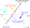 |
Fig. 9. Schematic sketch of the KH waves based on the average normal directions of the inbound and outbound crossings and the shear flow direction (maximum variance direction of V) in the R − T plane. The flow directions on Side 1 and Side 2 correspond to the velocity perturbation vectors outside the wave-like interval in Fig. 8f. The shear flow direction is nearly perpendicular to the wave edge normals, which can be interpreted as wavy structures developed within the velocity shear layer consistent with KH waves. |
Normal directions and orientations of the inbound and outbound crossings with their normal directions (n).
3.4. Magnetic spectra
We now examine turbulence properties of the KH event. Figure 10 shows the KH interval with KH subregions V1 to V6 highlighted with colors (middle) together with time periods before and after the KH interval (see top). Figure 10h shows a spectrogram of magnetic spectrum. The magnetic spectrum shows enhancement within the KH region compared to before or after the interval. The enhancement is visually strongest in V2 compared with other vortices. This V2 is the same interval as between (2) and (3) in Fig. 8 where we see a clear vortex-like rotation in the magnetic field and velocity field perturbations consistent with a rolled-up KH vortex. Thus, the strong enhancement in magnetic wave power provides evidence of enhanced activity in this vortex as plausibly facilitated by the development of a nonlinear KH vortex. The enhancement of the magnetic spectrum in V4 is also strong but less than for V2.
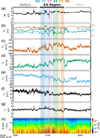 |
Fig. 10. Overview of the intervals for magnetic spectrum analysis. The KH region is marked in the middle (see top) together with the intervals before (top left) and after (top right). The KH vortices V1 to V6, marked between the compressed current sheets, are shaded in colors. (a) Total magnetic field. (b) Magnetic field in the RTN system. (c–e) Velocity field VR, VT, and VN components, respectively. (f) Ion number density. (g) Ion temperature. (h) Magnetic spectrum. |
To quantitatively assess the magnetic field fluctuations in the full KH region and in each of the six sub-regions V1 − V6 marked in Fig. 10, we computed magnetic field spectra for each interval, which are shown in Fig. 11. Additionally, the asymptotic regions immediately before and after the KH event are shown for reference. The vortex size is marked by an arrow (top left). The spectrum for the full KH region is shown in black while the spectra of the intervals before and after are shown in gray. As references, power law scalings of k−5/3 (Kolmogorov 1941) at MHD scales and k−2.8 at ion scales (e.g., Alexandrova et al. 2009) are plotted as black dashed lines. The scale of a thermal ion gyroradius (ρp) and an ion inertial length (dp) based on the average properties in the KH region are marked with vertical solid and dashed black lines, respectively. The spectrum of the entire KH interval has more power than the intervals before and after, which both have similar low-intensity spectra. This suggests that the KH waves are exciting additional fluctuations. The magnetic spectrum of the KH region approximately follows both power laws with a spectral breakpoint at f ∼ 0.2 Hz. The spectrum essentially follows the power law k−2.8 for scales smaller than the ion gyroradius. This indicates that the magnetic spectrum of the KH wave interval is consistent with a classic turbulence cascade down to the kinetic scales (e.g., Bruno et al. 2014, 2017). This result provides evidence of shear-driven turbulence as driven by the local KH waves.
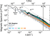 |
Fig. 11. Magnetic spectra of all regions marked in Fig. 10. The Kolmogorov power law k−5/3 and the dissipation range scalings k−2.8 are plotted for reference as black dashed straight lines. The vortex size is noted by an arrow (top left). The ion gyroradius scale (ρp) and the ion inertial length (dp) are marked by vertical black solid and dashed lines, respectively. |
Figure 11 also shows magnetic spectra for individual vortices V1 − V6. We note that the compressed current sheets are excluded for the analyses of these vortices (this is why the coloured regions are not exactly contiguous on Fig. 10). The powers of the magnetic spectra of all vortices are weaker than that of the entire KH region, indicating that the current sheets are key regions for enhancing the power spectrum. V2 (blue) and V4 (green) appear to have higher powers compared to other vortices and almost reach the power of the entire KH region (black). The enhanced power in these vortices may be related to the excitation of turbulent fluctuations through secondary instabilities and the nonlinear evolution of the KH instability. The difference in the power spectrum between the different vortices may indicate that SolO was crossing different parts of KH vortices while crossing through the shear layer from Side 1 to Side 2. It is likely that SolO was passing through the center of a rolled-up vortex in V2, for reasons noted earlier. The lower powers of V1, V5, and V6 may indicate that SolO was skimming through the trough or crest parts of KH vortices.
4. Discussion
We have reported observations of quasi-periodic magnetic field variations consistent with KH waves within a shear layer embedded in the slow solar wind close to an HCS using Solar Orbiter observations. The event is observed in the inner heliosphere at a distance of ∼0.69 AU. Our analysis of the observed conditions just outside the quasi-periodic interval reveals that the observed shear layer is not strictly consistent with an equilibrium tangential discontinuity (TD). The lack of equilibrium is likely due to the fact that the KH instability was generated at an upstream location before propagating to the observed location. Also, the development of the KH waves may have impacted the local equilibrium whose asymptotic conditions are not expected to strictly correspond to the initial TD conditions. Additionally, we note that nonlinear KH waves as observed in nature do not need to start with an equilibrium and infinitesimal perturbations as considered in linear theory. The observed shear layer has a complex 3D configuration that may not easily be reduced to a 1D or 2D problem although this is often done in literature (i.e., for KH observations at the magnetopause). Whether the KH instability can develop in such complex configuration should be investigated in future work.
Despite the lack of a proper frame that would provide parameters all consistent with classic 2D configurations, we have tested the stability of the shear layer with the linear theory using the assumption of an initial TD configuration at equilibrium and with boundary conditions similar to the observed asymptotic values. The linear theory analysis yields a positive growth rate, consistent with the KH instability development. We have also set up an MHD simulation with similar conditions and found that KH waves develop. We note that further investigations should be conducted to understand KH development in such complex magnetic and plasma configurations. Also, whether the KH dynamics may destroy a possibly pre-existing TD equilibrium after the KH instability reaches the nonlinear stage should also be investigated.
Apart from the nonzero normal magnetic field component in asymptotic parameters, there are all evidences that support the interpretation in terms of KH wave development, namely, (1) the significant velocity shear across the unstable surface with associated velocity perturbations, (2) the quasi-periodic magnetic field fluctuations consistent with KH waves, (3) the local conditions (albeit approximative) that are consistent with linear theory for the development of the KH instability, (4) the inbound/outbound boundary layer normal directions consistent with surface waves, (5) the simulation that shows the development of the KH for boundary conditions similar to that observed (albeit with an approximate initial condition as discussed above), and (6) the B and V perturbation patterns from the average showing interchanging directions within the wave interval as well as the vortex-like perturbation at one of the intervals consistent with a rolled-up KH vortex. To summarize, we believe that this event is consistent with the observation of KH waves. Several limitations should be further investigated as discussed above.
Despite several theoretical postulations (e.g., Parker 1963; Sturrock & Hartle 1966; Miura & Pritchett 1982; Korzhov et al. 1984; Neugebauer et al. 1986; Hollweg 1987) and spacecraft missions in the inner heliosphere, direct evidences for the KH waves were not reported in past in situ observations of the solar wind. We now focus on discussion on why this event may be favorable for a KH wave detection as well as implications of the KH dynamics in the solar wind as follows.
4.1. KH instability criterion in the solar wind
First, we consider solar wind conditions that are favorable for the KH instability. Based on the KH instability onset condition (Eq. (1)), the shear layer can more easily become unstable to the instability when B is low and n is high because it requires a velocity jump across the shear layer greater than the local Alfvén speed (ΔV > 2VA). Near the Sun, B and VA are typically large. This inhibitory effect on the KH instability criterion should be stronger near the Sun. Nevertheless, there may be several situations where the local conditions allow the KH instability. For example, remote sensing by DeForest et al. (2018) show a particularly strong shear values of a ΔVR ∼ 200 km s−1 across streamer structures in the young solar wind. Ruffolo et al. (2020) also propose the KH instability development near the Alfvén critical zone, at R < 0.17 AU. The event we analyze here was observed near the HCS with many coherent structures and shears at 0.69 AU. Besides, this event is found in the slow wind, which is generally dense, making the conditions to meet the KH instability criterion easier.
Second, we consider the magnetic and velocity field configurations across shear layers. The KH instability is suppressed when B is strong in the direction of ΔV due to the stabilization by magnetic tension in the direction of the shear flow. In this interplanetary medium, we typically expect a shear interface along the Parker spiral direction, so B may usually be aligned with ΔV. However, near the Sun, there may be velocity shear due to the solar-wind corotation with the Sun (e.g., Pinto et al. 2021). Several studies have shown that the KH instability may occur in various situations, for example, at the edge of a CME (e.g., Foullon et al. 2013; Möstl et al. 2013) and at the interfaces between CME and sheath and between sheath and solar wind (e.g., Páez et al. 2017).
Third, Eq. (1) is derived by assuming an ideal MHD plasma with an infinitely thin shear layer. In reality, nonideal MHD effects such as the compressibility can stabilize the KH instability (e.g., Sen 1964); for example, the KH instability only grows for a limited range of the velocity jump across a shear flow for a 1D TD in homogeneous plasmas and magnetic fields (e.g., Talwar 1964; Pu & Kivelson 1983). The out-of-plane magnetic field component, i.e., Bz, also plays an important role in the compressible regime, especially for the supersonic or super-magnetosonic environments (Miura 1990; Palermo et al. 2011a; Henri et al. 2012). The solar wind is indeed compressible and thus we expect some stabilizing effects. In addition, shear layers have finite thicknesses. A finite thickness of the shear layer can also stabilize the KH mode for small wavelength perturbations (i.e., for large wave number k). A combination of the compressibility and the finite thickness can stabilize the KH instability such that only certain modes of kΔL, where ΔL is the shear layer thickness, are KH-unstable (Miura & Pritchett 1982). Although these two factors can impact the shear-layer stability, we do not expect their effects to be large, nor to be specifically dependent on the distance from the Sun.
To summarize, there are factors that can impact the KH instability development in the solar wind. The magnitude of B and VA depend on distance from the Sun. As VA is higher closer to the Sun, the KH instability criterion should be more difficult to satisfy, except where the shear ΔV is particularly strong. Often B may be parallel to the velocity shear, tending to inhibit the KH instability, except in some circumstances, for example, when there is a CME that changes the local conditions. Compressibility of the solar wind and a finite thickness of the shear region can help stabilize the KH instability.
Since the observed conditions during our event are not particularly unusual for dense solar wind near the HCS, KH wave development should not be rare. We now consider arguments related to the KH timescale as follows.
4.2. KH timescale
A first fact to consider now is that when the KH instability develops at a shear layer, it quickly reaches the nonlinear stage (i.e., the rolled-up stage). The periodic features and vortical structures then get rapidly destroyed as the plasmas from either side of the shear layer mix and vortices coalesce. At such late stage, they would be indistinguishable from other solar wind types, albeit likely associated with higher levels of fluctuations as we have actually found in Sect. 3.4 for this event. The timescale for the decay of a KH vortex is on the order of one (γ−1) or a few folding times, e.g., 3γ−1. From the linear theory, we found that the maximum growth rate (γ/k) is about 16 km s−1 for the fastest growing mode (i.e., Walker 1981; Miura & Pritchett 1982). Using λ ∼ λKH, we obtain this timescale to be around 10 min. Since the conditions of our event are not unusual for dense solar wind near the HCS, this short timescale (i.e., on the order of minutes) for the vortex decay may contribute to the rarity of KH wave detection.
It is also possible that KH waves were detected by past missions but their signatures were not resolved. Several periodic oscillations in magnetic field strength were observed by Burlaga (1968) using the Pioneer-6 spacecraft, launched in 1965, at ∼0.8 AU. One of the cases considered was found to have sinusoidal |B| oscillations with a period of ∼5 min, embedded in a velocity shear layer. Although no other fluctuations were seen in the data, it was suggested that the empirical conditions taken as the boundary values marginally satisfy the KH instability criterion.
4.3. Implications of the KH waves in the solar wind
The KH waves are expected to play important roles, such as allowing for plasma mixing, generating turbulence, or producing Alfvénic fluctuations in the solar wind as mediated by KH vortex dynamics. During the present event, SolO observed an ion jet consistent with magnetic reconnection (see Sect. 2.4). An interesting question is whether this reconnection is produced due to dynamics of a KH vortex. For vortex-induced reconnection (VIR), we expect reconnection to be produced at a thin current sheet in between two vortices. At the Earth’s magnetopause, VIR jets were found to orient themselves along KH trailing edges (e.g., Eriksson et al. 2016) as the vortex evolves and further enhances the magnetic shear. In our case, we found that the jet is in the out-of-ecliptic direction (N) while the KH wave edges (see Table 3) and the shear layer are in the R, T directions. Thus, it is unclear whether the observed jet is a VIR. We think that the N-directed jet is rather a consequence of the inclination of the local current sheet. Nevertheless, the KH vortex may further increase the magnetic shear at the KH edge and make the current sheet thin enough to trigger magnetic reconnection.
We now discuss the magnetic and velocity field fluctuations. We found that the KH wave interval has enhanced fluctuations compared to outside the interval and the magnetic spectrum of the KH region approximately follows the power law scalings of k−5/3 and k−2.8 at inertial and kinetic scales, respectively (Sect. 3.4). These enhanced fluctuations are consistent with turbulence generation by the KH waves at the magnetopause (e.g., Stawarz et al. 2016; Nakamura et al. 2017). Therefore, the magnetic spectrum is consistent with a classical turbulence cascade down to the kinetic scales. These observations are consistent with an enhancement of turbulence in the solar wind as driven by the local KH waves (e.g., Goldstein et al. 1989). We also note that current sheets are key structures that contribute to the power spectrum, as power spectra of only vortex regions are lower than the overall spectrum. In addition, several of the vortices have enhanced power within them, which may be due to secondary instabilities, perhaps supporting the idea that the KH waves help to drive some fraction of the turbulent fluctuations in the solar wind.
One important implication of KH waves in the solar wind is that they can contribute to the evolution of the magnetic and velocity fluctuations. Near the Sun, the KH waves are believed to be a mechanism that leads to shear-driven turbulence at the Alfvén critical zone where V = VA and in the vicinity of the β = 1 surface (DeForest et al. 2016; Chhiber et al. 2018), leading to more isotropic solar-wind streams. Furthermore, the dynamical evolution invoked by shear-driven instabilities such as the KH waves is found to be able to account for features observed by PSP including magnetic “switchbacks” near perihelia (Ruffolo et al. 2020). This topic needs to be investigated further but it is beyond the scope of the present study.
5. Conclusions
We report observations of the KH waves with SolO on July 23, 2020 at 0.69 AU, during the cruise phase. The KH waves are observed within the velocity shear layer with periodic fluctuations in several parameters in the slow solar wind near an HCS. Several KH waveforms are observed with a period of ∼7 min but only a few vortices are clearly noticed. We tested the observed conditions on either side of the shear layer with linear theory using the TD and initial equilibrium assumptions. We note that these assumptions are made based on the consideration that (1) the KH waves were likely generated at an upstream location and (2) the KH wave development can alter the boundary conditions from the initial equilibrium, which may explain the observed nonzero magnetic field along the inhomogeneous direction of the shear layer observed at SolO. With these assumptions, we find that the shear layer is indeed unstable to the KH instability. Using linear theory, the wave phase speed is estimated to be 152 km s−1. The KH wavelength is approximately 66 400 km or 0.1 solar radii. We also confirm the local KH instability development by exploiting a 2D MHD simulation with the empirical values and the initial TD assumption.
Additionally, we report the observation of an ion jet consistent with magnetic reconnection at one of the wave edges, likely as a result of current sheet compression in between two KH vortices. The ion jet has ΔV = 11 km s−1 along the magnetic shear direction, consistent with magnetic reconnection but with a sub-Alfvénic jet. Nevertheless, we found other signatures consistent with magnetic reconnection, namely a drop in magnetic field strength, an ion number density enhancement (Gosling et al. 2005), and plasma heating (Phan et al. 2014). It is unclear whether this jet is produced due to KH vortex-induced reconnection (e.g., Nakamura et al. 2006) or the local inclination of the magnetic field, as the jet direction does not correspond to the KH wave edge direction (Eriksson et al. 2016).
We also report the enhancement of the magnetic and velocity field fluctuations within the KH activity interval compared to intervals outside. The power of the magnetic spectrum of the entire KH wave interval approximately follows the power law scalings of k−5.3 and k−2.8 in the inertial and kinetic ranges, respectively, consistent with the turbulent cascade in the solar wind. This provides evidence for the local enhancement of turbulence as driven by the KH activity. Moreover, we find that current sheets within the KH wave interval are key structures that enhance the power, as the magnetic spectra of individual KH vortices (excluding compressed current sheet intervals) generally have less power.
As our reported event here is an unambiguous in situ observation of the KH waves in the solar wind, we discuss possible reasons why the KH waves were not reported in past in situ observations. First, the KH instability onset criterion requires a velocity jump across the shear layer that is larger than twice the local Alfvén speed (ΔV > 2VA) and weak magnetic field in the direction of the shear flow (i.e., low B ⋅ ΔV). Second, the KH instability is estimated to quickly reach the nonlinear stage where KH vortices roll up and merge. This timescale should be on the order of a vortex decay time. The observed conditions are typical in the solar wind, and we estimate the timescale of the linear KH waves to be on the order of minutes. In other words, when KH instability develops in the solar wind, it evolves rapidly and is thus rather ephemeral.
This event provides evidence for the existence of the KH waves in the solar wind. It sheds new light on solar wind shear processes in the interplanetary medium with direct applications to shear-driven turbulence mediated by the KH waves, likely contributing to the solar wind fluctuations observed at 1 AU (e.g., Ruffolo et al. 2020). As the Alfvén speed decreases away from the Sun, the KH growth rate becomes higher (e.g., Neugebauer et al. 1986) and thus the KH waves may be more common. Due to the short timescale of the linear KH waves, there may be more chances to detect nonlinear KH structures or their remnants. Recently, techniques for detecting kinetic features of the KH waves during the nonlinear and turbulent stage of the KH instability were proposed (Settino et al. 2021). Further studies would be needed to study secondary processes induced by the KH instability in the solar wind such as vortex-induced reconnection and other kinetic mechanisms, as the KH structures are rich with magnetic and plasma structures as are well known for the case of the magnetopause.
Acknowledgments
The authors acknowledge the reviewer’s constructive and helpful comments. Work at IRAP and LAB was supported by the Centre National de la Recherche Scientifique (CNRS, France), the Centre National d’Etudes Spatiales (CNES, France), the Université Paul Sabatier (UPS), and the Université de Bordeaux. Solar Orbiter data are publicly available at http://soar.esac.esa.int/soar/. We acknowledge science teams of the Connectivity Tool (http://connect-tool.irap.omp.eu/) and 3DView (http://3dview.irap.omp.eu/) at IRAP and CNES. Y.Y. is supported by grant No. 11902138 from the National Natural Science Foundation of China. The computing resources were provided by the Center for Computational Science and Engineering of Southern University of Science and Technology. D.R. is supported by grant RTA6280002 from Thailand Science Research and Innovation. J.E.S. is supported by the Royal Society University Research Fellowship URF/R1/201286. C.J.O. is funded under STFC grant number ST/5000240/1. Solar Orbiter Solar Wind Analyser (SWA) data are derived from scientific sensors which have been designed and created, and are operated under funding provided in numerous contracts from the UK Space Agency (UKSA), the UK Science and Technology Facilities Council (STFC), the Agenzia Spaziale Italiana (ASI), the CNES, the CNRS, the Czech contribution to the ESA PRODEX programme and NASA. Solar Orbiter SWA work at UCL/MSSL is currently funded under STFC grants ST/T001356/1 and ST/S000240/1.
References
- Alexandrova, O., Saur, J., Lacombe, C., et al. 2009, Phys. Rev. Lett., 103, 165003 [NASA ADS] [CrossRef] [Google Scholar]
- Arge, C. N., Henney, C. J., Koller, J., et al. 2010, in Twelfth International Solar Wind Conference, eds. M. Maksimovic, K. Issautier, N. Meyer-Vernet, M. Moncuquet, & F. Pantellini, AIP Conf. Ser., 1216, 343 [NASA ADS] [Google Scholar]
- Axford, W. I., & McKenzie, J. F. 1992, in Solar Wind Seven Colloquium, eds. E. Marsch, & R. Schwenn, 1 [Google Scholar]
- Borovsky, J. E. 2008, J. Geophys. Res.: Space Phys., 113, A08110 [NASA ADS] [Google Scholar]
- Bruno, R., & Carbone, V. 2005, Liv. Rev. Sol. Phys., 2, 4 [Google Scholar]
- Bruno, R., Trenchi, L., & Telloni, D. 2014, ApJ, 793, L15 [NASA ADS] [CrossRef] [Google Scholar]
- Bruno, R., Telloni, D., DeIure, D., & Pietropaolo, E. 2017, MNRAS, 472, 1052 [NASA ADS] [CrossRef] [Google Scholar]
- Burlaga, L. F. 1968, Sol. Phys., 4, 67 [Google Scholar]
- Burlaga, L. F. 1969, Sol. Phys., 7, 54 [Google Scholar]
- Burlaga, L. F. 1972, in Microstructure of the Interplanetary Medium, eds. C. P. Sonett, P. J. Coleman, & J. M. Wilcox, 308, 309 [NASA ADS] [Google Scholar]
- Burlaga, L. F., Lemaire, J. F., & Turner, J. M. 1977, J. Geophys. Res., 82, 3191 [NASA ADS] [CrossRef] [Google Scholar]
- Chandrasekhar, S. 1961, Hydrodynamic and Hydromagnetic Stability (Oxford: Clarendon Press) [Google Scholar]
- Chhiber, R., Usmanov, A. V., DeForest, C. E., et al. 2018, ApJ, 856, L39 [Google Scholar]
- De Pontieu, B., Title, A. M., Lemen, J. R., et al. 2014, Sol. Phys., 289, 2733 [Google Scholar]
- DeForest, C. E., Matthaeus, W. H., Viall, N. M., & Cranmer, S. R. 2016, ApJ, 828, 66 [Google Scholar]
- DeForest, C. E., Howard, R. A., Velli, M., Viall, N., & Vourlidas, A. 2018, ApJ, 862, 18 [Google Scholar]
- Eriksson, S., Lavraud, B., Wilder, F. D., et al. 2016, Geophys. Res. Lett., 43, 5606 [CrossRef] [Google Scholar]
- Fairfield, D. H., Otto, A., Mukai, T., et al. 2000, J. Geophys. Res., 105, 21,159 [Google Scholar]
- Fairfield, D. H., Kuznetsova, M. M., Mukai, T., et al. 2007, J. Geophys. Res.: Space Phys., 112, 1 [Google Scholar]
- Fargette, N., Lavraud, B., Rouillard, A. P., et al. 2021, A&A, 650, A11 [NASA ADS] [CrossRef] [EDP Sciences] [Google Scholar]
- Foullon, C., Farrugia, C., Fazakerley, A., et al. 2008, J. Geophys. Res.: Space Phys., 113, A11203 [Google Scholar]
- Foullon, C., Verwichte, E., Nakariakov, V. M., Nykyri, K., & Farrugia, C. J. 2011, ApJ, 729, 2 [Google Scholar]
- Foullon, C., Verwichte, E., Nykyri, K., Aschwanden, M. J., & Hannah, I. G. 2013, ApJ, 767, 170 [Google Scholar]
- Fox, N. J., Velli, M. C., Bale, S. D., et al. 2016, Space Sci. Rev., 204, 7 [Google Scholar]
- Génot, V., Beigbeder, L., Popescu, D., et al. 2018, Planet. Space Sci., 150, 111 [CrossRef] [Google Scholar]
- Goldstein, M. L., Roberts, D. A., & Matthaeus, W. H. 1989, Washington DC American Geophysical Union Geophysical Monograph Series, 54, 113 [NASA ADS] [Google Scholar]
- Gosling, J. T., & Phan, T. D. 2013, ApJ, 763, 1987 [Google Scholar]
- Gosling, J. T., Skoug, R. M., McComas, D. J., & Smith, C. W. 2005, J. Geophys. Res.: Space Phys., 110, A01107 [NASA ADS] [CrossRef] [Google Scholar]
- Haggerty, C. C., Shay, M. A., Chasapis, A., et al. 2018, Phys. Plasmas, 25, 102120 [Google Scholar]
- Hasegawa, A. 1975, Plasma Instabilities and Nonlinear Effects (New York: Springer-Verlag) [CrossRef] [Google Scholar]
- Hasegawa, H., Fujimoto, M., Phan, T.-D., et al. 2004, Nature, 430, 755 [NASA ADS] [CrossRef] [Google Scholar]
- Henri, P., Califano, F., Faganello, M., & Pegoraro, F. 2012, Phys. Plasmas, 19, 072908 [NASA ADS] [CrossRef] [Google Scholar]
- Hickmann, K. S., Godinez, H. C., Henney, C. J., & Arge, C. N. 2015, Sol. Phys., 290, 1105 [NASA ADS] [CrossRef] [Google Scholar]
- Hillier, A., & Polito, V. 2018, ApJ, 864, L10 [Google Scholar]
- Hollweg, J. V. 1982, J. Geophys. Res., 87, 8065 [CrossRef] [Google Scholar]
- Hollweg, J. V. 1987, ApJ, 317, 918 [NASA ADS] [CrossRef] [Google Scholar]
- Hones, E. W., Birn, J., Bame, S. J., et al. 1981, J. Geophys. Res., 86, 814 [NASA ADS] [CrossRef] [Google Scholar]
- Horbury, T. S., O’Brien, H., Carrasco Blazquez, I., et al. 2020, A&A, 642, A1 [NASA ADS] [CrossRef] [EDP Sciences] [Google Scholar]
- Hudson, P. D. 1970, Planet. Space Sci., 18, 1611 [Google Scholar]
- Kacem, I., Jacquey, C., Génot, V., et al. 2018, J. Geophys. Res.: Space Phys., 123, 1779 [NASA ADS] [Google Scholar]
- Karimabadi, H., Roytershteyn, V., Wan, M., et al. 2013, Phys. Plasmas, 20, 012303 [Google Scholar]
- Kieokaew, R. 2019, PhD Thesis, University of Exeter [Google Scholar]
- Kieokaew, R., Lavraud, B., Foullon, C., et al. 2020, J. Geophys. Res.: Space Phys., 125, 1 [Google Scholar]
- Knetter, T., Neubauer, F. M., Horbury, T., & Balogh, A. 2004, J. Geophys. Res.: Space Phys., 109, A06102 [NASA ADS] [CrossRef] [Google Scholar]
- Kolmogorov, A. 1941, Akademiia Nauk SSSR Doklady, 30, 301 [Google Scholar]
- Korzhov, N. P., Mishin, V. V., & Tomozov, V. M. 1984, Planet. Space Sci., 32, 1169 [NASA ADS] [CrossRef] [Google Scholar]
- Landau, L. D., & Lifshitz, E. M. 1987, Fluid Mechanics (Oxford: Pergamon Press) [Google Scholar]
- Lepping, R. P., & Behannon, K. W. 1986, J. Geophys. Res., 91, 8725 [NASA ADS] [CrossRef] [Google Scholar]
- Louarn, P. 2004, Geophys. Res. Lett., 31, L19805 [NASA ADS] [CrossRef] [Google Scholar]
- Matthaeus, W. H., & Goldstein, M. L. 1982, J. Geophys. Res., 87, 6011 [Google Scholar]
- Miura, A. 1990, Geophys. Res. Lett., 17, 749 [NASA ADS] [CrossRef] [Google Scholar]
- Miura, A., & Pritchett, P. L. 1982, J. Geophys. Res., 87, 7431 [NASA ADS] [CrossRef] [Google Scholar]
- Möstl, U. V., Temmer, M., & Veronig, A. M. 2013, ApJ, 766, L12 [Google Scholar]
- Müller, D., St. Cyr, O. C., Zouganelis, I., et al. 2020, A&A, 642, A1 [Google Scholar]
- Nakamura, T. K. M., Fujimoto, M., & Otto, A. 2006, Geophys. Res. Lett., 33, L14106 [NASA ADS] [CrossRef] [Google Scholar]
- Nakamura, T. K. M., Hasegawa, H., Daughton, W., et al. 2017, Nat. Commun., 8, 1582 [NASA ADS] [CrossRef] [Google Scholar]
- Neugebauer, M. 1985, J. Geophys. Res., 90, 6627 [NASA ADS] [CrossRef] [Google Scholar]
- Neugebauer, M. 2006, J. Geophys. Res.: Space Phys., 111, A04103 [NASA ADS] [Google Scholar]
- Neugebauer, M., & Giacalone, J. 2010, AIP Conf. Proc., 1216, 194 [CrossRef] [Google Scholar]
- Neugebauer, M., Clay, D. R., Goldstein, B. E., Tsurutani, B. T., & Zwickl, R. D. 1984, J. Geophys. Res., 89, 5395 [Google Scholar]
- Neugebauer, M., Alexander, C. J., Schwenn, R., & Richter, A. K. 1986, J. Geophys. Res., 91, 13694 [CrossRef] [Google Scholar]
- Nykyri, K., & Otto, A. 2001, Geophys. Res. Lett., 28, 3565 [NASA ADS] [CrossRef] [Google Scholar]
- Ofman, L., & Thompson, B. J. 2011, ApJ, 734, L11 [Google Scholar]
- Øieroset, M., Phan, T. D., Drake, J. F., et al. 2019, Geophys. Res. Lett., 46, 1937 [Google Scholar]
- Owen, C. J., Bruno, R., Livi, S., et al. 2020, A&A, 642, A16 [EDP Sciences] [Google Scholar]
- Páez, A., Jatenco-Pereira, V., Falceta-Gonçalves, D., & Opher, M. 2017, ApJ, 851, 112 [CrossRef] [Google Scholar]
- Palermo, F., Faganello, M., Califano, F., Pegoraro, F., & Le Contel, O. 2011a, J. Geophys. Res.: Space Phys., 116, 1 [Google Scholar]
- Palermo, F., Faganello, M., Califano, F., & Pegoraro, F. 2011b, Ann. Geophys., 29, 1169 [NASA ADS] [CrossRef] [Google Scholar]
- Papamoschou, D., & Roshko, A. 1988, J. Fluid Mech., 197, 453 [NASA ADS] [CrossRef] [Google Scholar]
- Parker, E. N. 1958, ApJ, 128, 664 [Google Scholar]
- Parker, E. N. 1963, Interplanetary Dynamical Processes (Interscience Publishers: New York) [Google Scholar]
- Paschmann, G., Papamastorakis, I., Baumjohann, W., et al. 1986, J. Geophys. Res., 91, 11099 [NASA ADS] [CrossRef] [Google Scholar]
- Phan, T. D., Drake, J. F., Shay, M. A., et al. 2014, Geophys. Res. Lett., 41, 7002 [Google Scholar]
- Pinto, R. F., Poirier, N., Rouillard, A. P., et al. 2021, A&A, 653, A92 [NASA ADS] [CrossRef] [EDP Sciences] [Google Scholar]
- Pu, Z.-Y., & Kivelson, M. G. 1983, J. Geophys. Res., 88, 841 [NASA ADS] [CrossRef] [Google Scholar]
- Roberts, D. A., Goldstein, M. L., Matthaeus, W. H., & Ghosh, S. 1992, J. Geophys. Res., 97, 17115 [Google Scholar]
- Roudier, T., & Muller, R. 1986, Sol. Phys., 107, 11 [NASA ADS] [CrossRef] [Google Scholar]
- Rouillard, A. P., Pinto, R. F., Vourlidas, A., et al. 2020, A&A, 642, A2 [NASA ADS] [CrossRef] [EDP Sciences] [Google Scholar]
- Ruffolo, D., Matthaeus, W. H., Chhiber, R., et al. 2020, ApJ, 902, 94 [Google Scholar]
- Sen, A. K. 1964, Phys. Fluids, 7, 1293 [Google Scholar]
- Settino, A., Perrone, D., Khotyaintsev, Y. V., Graham, D. B., & Valentini, F. 2021, ApJ, 912, 154 [NASA ADS] [CrossRef] [Google Scholar]
- Siscoe, G. L., & Suey, R. W. 1972, J. Geophys. Res., 77, 1321 [NASA ADS] [CrossRef] [Google Scholar]
- Sonnerup, B. U. Ö., & Cahill, L. J. 1967, J. Geophys. Res., 72, 171 [NASA ADS] [CrossRef] [Google Scholar]
- Stawarz, J. E., Eriksson, S., Wilder, F. D., et al. 2016, J. Geophys. Res.: Space Phys., 121, 11,021 [Google Scholar]
- Sturrock, P. A., & Hartle, R. E. 1966, Phys. Rev. Lett., 16, 628 [CrossRef] [Google Scholar]
- Talwar, S. P. 1964, J. Geophys. Res., 69, 2707 [NASA ADS] [CrossRef] [Google Scholar]
- Tsurutani, B. T., & Smith, E. J. 1979, J. Geophys. Res., 84, 2773 [Google Scholar]
- Walker, A. D. M. 1981, Planet. Space Sci., 29, 1119 [NASA ADS] [CrossRef] [Google Scholar]
- Yang, Y., Wan, M., Shi, Y., Yang, K., & Chen, S. 2016a, J. Comput. Phys., 306, 73 [NASA ADS] [CrossRef] [Google Scholar]
- Yang, Y., Shi, Y., Wan, M., Matthaeus, W. H., & Chen, S. 2016b, Phys. Rev. E, 93, 061102 [NASA ADS] [CrossRef] [Google Scholar]
- Yang, Y., Matthaeus, W. H., Shi, Y., Wan, M., & Chen, S. 2017, Phys. Fluids, 29, 035105 [CrossRef] [Google Scholar]
- Zaqarashvili, T. V., Vörös, Z., & Zhelyazkov, I. 2014, A&A, 561, A62 [NASA ADS] [CrossRef] [EDP Sciences] [Google Scholar]
All Tables
Normal directions and orientations of the inbound and outbound crossings with their normal directions (n).
All Figures
|
Fig. 1. Overview of SolO and other spacecraft positions on 23 July 2020 at 20:01:08 UT projected in a solar equatorial plane in the RTN coordinates centered at SolO. Orange solid lines represent solar wind Parker spirals (Parker 1958) calculated using a constant velocity of 300 km s−1. This figure was obtained using the 3DView software (Génot et al. 2018). |
| In the text | |
|
Fig. 2. Connectivity map of the observations on July 23, 2020, produced from the Connectivity Tool (Rouillard et al. 2020) to provide a global context. The background is a combined image from remote observation using SDO/AIA and STEREO-A/EUVI 171 Å Carrington maps. The blue cross represents the region of high connectivity probability of SolO to the solar wind source regions. The green and red dots represent zones of the high connectivity probability to the solar wind source regions assuming fast and slow winds, respectively. The heliospheric current sheet (HCS) is marked with a red dashed line. |
| In the text | |
|
Fig. 3. Solar Orbiter observations between 16:00 UT on 23 July 2020 and 6:00 UT on 24 July 2020 showing the context of the Kelvin-Helmholtz instability observation (shaded area). (a) Magnetic fields in the RTN coordinates. (b) Ion bulk velocity VR component. (c) Ion bulk velocity VT and VN components. (d) Ion number density. (e) Alfvén Mach number. (f) Normalized cross-helicity. (g) The angle between δV and B (see text). The heliospheric current sheet (HCS) is observed between 22:00 UT on 23 July 2020 and 2:00 UT on 24 July 2020, marked by purple dotted lines. The Magnetic Increase with Central Current Sheet (MICCS) is observed between 17:35 and 18:08 UT on 23 July 2020, marked by orange dotted lines. |
| In the text | |
|
Fig. 4. Solar Orbiter observations on 23 July 2020 between 20:10 UT and 21:50 UT. (a) Magnetic field in the RTN coordinates. (b) Ion bulk velocity VR component. (c) Ion bulk velocity VT and VN components. (d) Alfvén speed |VA| and Alfvén velocity components (VA, R, VA, T, VA, N). (e) Ion number density. (f) Plasma pressure Pp, magnetic pressure Pm, and total pressure Ptot. (g) Plasma beta β. The KH waves can be noticed between 20:45 and 21:30 UT. The vertical gray dashed lines (1)–(7) mark the boundary layer crossings corresponding to KH trailing edges. The magenta dashed-dotted lines mark times when the plasma parameters reach asymptotic values on Side 1 (20:38 UT) and Side 2 (21:29 UT) of the shear layer. |
| In the text | |
|
Fig. 5. Magnetic reconnection signatures at wave edge (3) in Fig. 4. (a) Magnetic field strength. (b) Magnetic field reconnecting |
| In the text | |
|
Fig. 6. Magnetic and velocity fields in the local shear frame obtained from the application of the MVA to the ion bulk velocity. (a) Magnetic field in the maximum (X), intermediate (Y), and minimum (Z) variance directions and its magnitude. (b–d) Velocity field in the X, Y, and Z directions, respectively. (e) Simplified shear boundary layer configuration obtained from the transformation to the maximum shear frame. |
| In the text | |
|
Fig. 7. Snapshot of the numerical simulation of the KH instability using empirical values of the SolO event from Side 1 and Side 2 with the initial TD assumption. The color-scale represents values of the out-of-plane flow vorticity (ω). The KH instability quickly reaches the nonlinear stage where rolled-up KH vortices form and coalesce. The stripes in vorticity in the lower part of the simulation are shocks (known as vortex-induced shocks) produced by the supersonic flow as the Mach number on this side is ∼3 (see text). |
| In the text | |
|
Fig. 8. Magnetic and velocity fields with their perturbations from the average shown with time progresses from right to left. Inbound and outbound crossings are marked with purple and cyan vertical dashed lines, respectively. (a) Magnetic fields. (b,c) Magnetic field fluctuations from the averages in the R − T and R − N planes, respectively. (d) Ion bulk velocity VR component. (e) Ion bulk velocity VT and VN components. (f,g) Velocity field perturbations in the R − T and R − N planes, respectively. |
| In the text | |
|
Fig. 9. Schematic sketch of the KH waves based on the average normal directions of the inbound and outbound crossings and the shear flow direction (maximum variance direction of V) in the R − T plane. The flow directions on Side 1 and Side 2 correspond to the velocity perturbation vectors outside the wave-like interval in Fig. 8f. The shear flow direction is nearly perpendicular to the wave edge normals, which can be interpreted as wavy structures developed within the velocity shear layer consistent with KH waves. |
| In the text | |
|
Fig. 10. Overview of the intervals for magnetic spectrum analysis. The KH region is marked in the middle (see top) together with the intervals before (top left) and after (top right). The KH vortices V1 to V6, marked between the compressed current sheets, are shaded in colors. (a) Total magnetic field. (b) Magnetic field in the RTN system. (c–e) Velocity field VR, VT, and VN components, respectively. (f) Ion number density. (g) Ion temperature. (h) Magnetic spectrum. |
| In the text | |
|
Fig. 11. Magnetic spectra of all regions marked in Fig. 10. The Kolmogorov power law k−5/3 and the dissipation range scalings k−2.8 are plotted for reference as black dashed straight lines. The vortex size is noted by an arrow (top left). The ion gyroradius scale (ρp) and the ion inertial length (dp) are marked by vertical black solid and dashed lines, respectively. |
| In the text | |
Current usage metrics show cumulative count of Article Views (full-text article views including HTML views, PDF and ePub downloads, according to the available data) and Abstracts Views on Vision4Press platform.
Data correspond to usage on the plateform after 2015. The current usage metrics is available 48-96 hours after online publication and is updated daily on week days.
Initial download of the metrics may take a while.