| Issue |
A&A
Volume 669, January 2023
|
|
|---|---|---|
| Article Number | A35 | |
| Number of page(s) | 8 | |
| Section | The Sun and the Heliosphere | |
| DOI | https://doi.org/10.1051/0004-6361/202244662 | |
| Published online | 03 January 2023 | |
High-energy particle enhancements in the solar wind upstream Mercury during the first BepiColombo flyby: SERENA/PICAM and MPO-MAG observations
1
INAF-Istituto di Astrofisica e Planetologia Spaziali, via del Fosso del Cavaliere 100, 00133 Rome, Italy
e-mail: This email address is being protected from spambots. You need JavaScript enabled to view it.
2
University of Michigan, Department of Climate and Space Sciences and Engineering, 2455 Hayward St, Ann Arbor, 48109 MI, USA
3
Space Research Institute, Austrian Academy of Sciences, Schmiedlstraße 6, 8042 Graz, Austria
4
Institut für Geophysik und Extraterrestrische Physik, Technische Universität Braunschweig, Mendelssohnstr. 3, 38106 Braunschweig, Germany
5
Swedish Institute of Space Physics, Bengt Hultqvists väg 1, 981 92 Kiruna, Sweden
6
Institut de Recherche en Astrophysique et Planétologie, CNRS, CNES, Université de Toulouse, 9 Av. du Colonel Roche, 31400 Toulouse, France
7
Aalto University, Department of Electronics and Nanoengineering, School of Electrical Engineering Helsinki, Maarintie 13, 02150 Helsinki, Finland
8
Southwest Research Institute, 6220 Culebra Rd, San Antonio, 78238 TX, USA
9
Italian Space Agency, Via del Politecnico, 00133 Roma, Italy
10
University of Bern, Institute of Physics, Hochschulstrasse, 4, 3021 Bern, Switzerland
11
Finnish Meteorological Institute, Erik Palménin aukio 1, 00560 Helsinki, Finland
Received:
2
August
2022
Accepted:
20
November
2022
Abstract
Context. The first BepiColombo Mercury flyby offered the unique opportunity to simultaneously characterize the plasma and the magnetic field properties of the solar wind in the vicinity of the innermost planet of the Solar System (0.4 AU).
Aims. In this study, we use plasma observations by SERENA/PICAM and magnetic field measurements by MPO-MAG to characterize the source with intermittent features (with a timescale of a few minutes) at ion energies above 1 keV observed in the solar wind upstream of Mercury.
Methods. The solar wind properties have been investigated by means of low-resolution magnetic field (1 s) and plasma (64 s) data. The minimum variance analysis and the Lundquist force-free model have been used.
Results. The combined analyses demonstrate that the intermittent ion features observed by PICAM at energies above 1 keV can be associated with the passage of an interplanetary magnetic flux rope. We also validate our findings by means of Solar Orbiter observations at a larger distance (0.6 AU).
Conclusions. The core of an interplanetary magnetic flux rope, hitting BepiColombo during its first Mercury flyby, produced high-energy (> -pagination1 keV) intermittent-like particle acceleration clearly distinct from the background solar wind, while at the edges of this interplanetary structure compressional low-energy fluctuations have also been observed.
Key words: solar wind / Sun: magnetic fields / plasmas
© The Authors 2023
 Open Access article, published by EDP Sciences, under the terms of the Creative Commons Attribution License (https://creativecommons.org/licenses/by/4.0), which permits unrestricted use, distribution, and reproduction in any medium, provided the original work is properly cited.
This article is published in open access under the Subscribe-to-Open model. This email address is being protected from spambots. You need JavaScript enabled to view it. to support open access publication.
1. Introduction
The interplanetary medium is permeated by an ionized gas, that is the solar wind plasma, flowing away from the Sun’s upper atmosphere (i.e., the solar corona) and carrying out mostly protons, electrons, and α particles (i.e., He++), together with a large-scale solar magnetic field (Gurnett & Bhattacharjee 2005). Since the era of space missions (1970s), the main features of the solar wind have been traced out: it has a mean flow speed around 400–450 km s−1; its density varies from 50 to 60 cm−3 (close to the Sun, Sarantos et al. 2007) to a few particles per cubic centimetres (close to the Earth and beyond); its proton temperature varies between 105 eV and 8 × 10⁵ eV; and the magnetic field magnitude scales with the distance from the Sun (R) as B0 R−2, with B0 ∼ 150 nT close to the Sun (Tu & Marsch 1990; Verscharen et al. 2019; Chen et al. 2020; Alberti et al. 2020; Telloni et al. 2021; Sun et al. 2022). When interacting with a planetary magnetic field or atmosphere, a planetary magnetosphere or induced magnetosphere would be formed, and the solar wind initiates many fundamental plasma processes, for example, transferring energy, mass, and momentum to the planetary magnetosphere (Akasofu 2021; Slavin et al. 2021), triggering plasma instabilities at the boundaries (Slavin et al. 2009), and so on.
Despite these continuous interactions, the interplanetary medium is also sometimes permeated by transient solar structures emitted directly from the solar surface and upper atmosphere, such as coronal mass ejections (CMEs), interplanetary shocks, and magnetic flux ropes (FRs; Temmer 2021; Foullon & Malandraki 2018). These structures carry out a huge amount of energy and mass, thus producing space weather events on planetary environments as magnetic storms, magnetospheric substorms, etc. The space weather events would energize particles, inject energetic particles into low altitude, increase electromagnetic radiation, and eventually produce hazards for spacecraft, infrastructures, and human life (Bothmer & Daglis 2007). Typically, solar transient events such as CMEs and FRs interact with the ambient solar wind and can be accelerated or decelerated during their time spent travelling within the interplanetary space. The interaction between the FRs and their ambient solar wind would generate compression regions and in situ phenomena-like shocks, instabilities, and particle accelerations.
On 01 October 2021 BepiColombo made its first encounter with Mercury, passing through the dusk flank of the magnetopause, entering the inner equatorial magnetosphere, and exiting from the dayside (Mangano et al. 2021; Benkhoff et al. 2021). Among operating instruments, the fluxgate magnetometer (MPO/MAG) and the ion camera (SERENA/PICAM) jointly collected data in the upstream solar wind and in the inner magnetosphere of Mercury (Orsini et al. 2022).
In this work, we use plasma observations by SERENA/PICAM and magnetic field measurements by MPO-MAG to characterize the source of these intermittent ion features (with a timescale of a few minutes) observed at energies above 1 keV in the solar wind upstream of Mercury (Sect. 2). By applying the minimum variance analysis and the Lundquist force-free fitting model (see Sect. 3), we are able to demonstrate that these intermittent features can be associated with the passage of an interplanetary magnetic FR. Furthermore, by making use of a radial alignment between BepiColombo and Solar Orbiter, with the latter being located at a larger distance (0.6 AU compared to 0.4 AU), we are able to validate our findings as to the FR occurrence as well as to derive its main features in the expanding phase. This study represents the first case study of a magnetic FR observed simultaneously close to Mercury and further away and it shows the potential of multi-spacecraft investigations for detecting solar transient events (Mangano et al. 2021; Möstl et al. 2022).
2. Data
Figure 1 reports the trajectory of the first BepiColombo flyby to Mercury in the XMSO–ρMSO plane. The Mercury Solar Orbital (MSO) coordinate system has its origin at the centre of Mercury with the X-axis being positive in the solar direction, the Z-axis is along the planetary rotation axis, and the Y-axis is positive opposite to the direction of Mercury’s orbital velocity completing the right-handed system ( ). The red line corresponds to the time interval considered in this study when BepiColombo sampled the upstream solar wind near Mercury when joint investigations between PICAM and MPO-MAG were possible. The grey line represents the average bow shock surface (Slavin et al. 2009; Winslow et al. 2013).
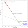 |
Fig. 1. Trajectory (dashed-dotted black line) of the first BepiColombo flyby to Mercury in the XMSO–ρMSO plane in units of the radius of Mercury, RM = 2439.7 km (the black arrow marks the spacecraft direction). The red line corresponds to the time interval considered in this study corresponding to PICAM measurements and when BepiColombo sampled the solar wind near Mercury. The grey line represents the average bow shock surface (Slavin et al. 2009; Winslow et al. 2013). The inbound and outbound bow shock crossings are marked by blue text. |
We used BepiColombo magnetometer data at 1-s resolution by the MPO-MAG instrument (Glassmeier et al. 2010; Heyner et al. 2021) and plasma observations at 64-s resolution from the PICAM unit (Orsini et al. 2010, 2021) of the first Mercury flyby on 01 October 2021 to simultaneously characterize the plasma and the magnetic field properties of the solar wind. Complimentary to the magnetic field components, we also evaluated the cone θc and clock ϕc angles of the magnetic field as follows:
 (1)
(1)
 (2)
(2)
They are useful parameters to characterize the direction of the interplanetary magnetic field. Specifically, when θc = 0° or θc = 180°, the magnetic field is sunward or anti-sunward, while θc = 90° implies a perpendicular field to the Mercury–Sun line. Additionally, ϕc shows the direction in the plane perpendicular to the Mercury–Sun line, with ϕc = 0° (90° ) indicating a field in the YMS0 − ZMSO direction. We also used Solar Orbiter magnetometer data at 1-s resolution by the Solo/MAG instrument (Horbury et al. 2020). Figure 2 reports the magnetic field measurements (middle), the cone θc and the clock ϕc angles (bottom), and the omni-directional time-energy ion counts (top).
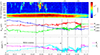 |
Fig. 2. Omni-directional time–energy ion counts (top), magnetic field measurements (middle), and cone θc and clock ϕc angles (bottom). The vertical dashed-dotted lines indicate the time intervals of interest marked by (1), (2), and (3), respectively. The horizontal dotted line in the bottom panel refers to the Parker spiral angle θP, while the arrow marks the rotation of the magnetic field. |
The omni-directional distribution observed by PICAM highlights a quite warm, dense, and low energy (peaking at about 600 eV) solar wind. This would correspond to a slow solar wind with a speed around 340 km s−1. An interesting feature observed by the ion camera was the occurrence of > -pagination1-keV ion enhancements, mostly directed in the opposite direction to the solar wind plasma (see Fig. 3), in close correspondence with the pointing of the SERENA/PICAM boresight towards the flank of the bow shock. Indeed, the SERENA/PICAM boresight rotated during the time interval moving from a perpendicular direction to the solar wind plasma flow, passing through the parallel direction. Two likely candidates can be the source of the high-energy particle enhancements observed in the upstream solar wind: on the one hand, dynamical processes occurring in the near-Mercury electromagnetic environment (as foreshock ions are transported upstream along the magnetic field lines); on the other hand, a solar transient event such as a CME or a magnetic FR. Furthermore, around 20:40 UT and 21:00 UT, low-energy ion enhancements were also observed. These three intervals (marked by (1), (2), and (3) in Fig. 2) are considered in this study.
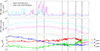 |
Fig. 3. High-energy (> 1 keV, top) and low-energy (< 1 keV, middle) ion counts in the solar wind direction (cyan lines) and in its opposite direction (magenta lines). Bottom: magnetic field measurements. The vertical dashed-dotted lines indicate the time intervals of interest (see Fig. 2). |
Simultaneous magnetic field measurements seem to suggest that the high-energy intermittent features are not correlated with magnetic signatures (e.g., wave-like activity, bursts, etc.), while the low-energy enhancements occur jointly with wave-like signatures and instabilities. By looking at the cone angle θc, we can observe that the Interplanetary Magnetic Field (IMF) is less radial than nominal between 19:01 and 20:30 UT, decreasing from θc ∼ 90° to θc ∼ θP, with θP being the Parker spiral angle. Then, the field remains spirally aligned, that is θc ∼ θP up to ∼21:05 UT. After that, it tilts between the anti-sunward and the perpendicular direction. The clock angle ϕc is mainly eastwards between 19:01 and 20:10 UT, rotating northwards around 20:15 UT, then switching again between eastwards (20:30–21:05 UT) and northwards (21:05–21:15 UT).
3. Results and discussions
We provide a deeper investigation of the observed features by focussing on the three time intervals separately.
3.1. Interval (1) 19:51–20:03: High-energy ions
Intermittent-like high-energy enhancements are observed by PICAM when the magnetic field pointed northwards (ϕc ∼ 90°) during a clear eastward-northward-eastward magnetic field rotation lasting from 19:00 UT to 20:30 UT. This rotation could be attributed to the passage of an interplanetary magnetic field structure, a magnetic cloud, or a magnetic FR, producing high-energy particle acceleration with respect to the background solar wind (peaking at about 600 eV). A magnetic cloud is usually associated with a CME, while a magnetic FR is a small, transient event (Burlaga 1988). Since no CMEs were erupting from the Sun on the previous day, the most probable candidate remains a FR. A typical signature of this structure is an increase in the average magnetic field magnitude (with respect to the main background field), a decrease in the variance of magnetic field fluctuations, and a smooth change in polarity in one of the field components (Moldwin et al. 2000). They last from a few minutes to a few hours and may be able to accelerate particles (le Roux et al. 2018). The smooth rotation has been observed in the clock angle ϕc and it mainly corresponds to a rotation of the By, MSO (see Fig. 2). To assess the other two features, we report the behaviour of the magnetic field intensity and the ratio between magnetic field fluctuations and its modulus in Fig. 4.
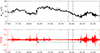 |
Fig. 4. Behaviour of the magnetic field intensity B (black line) and the ratio between magnetic field fluctuations and its modulus δB/B (red line). The arrow marks the rotation of the magnetic field. |
We clearly observe an enhancement in the intensity of the magnetic field and, at the same time, a decrease in its fluctuation level, thus confirming our initial speculation as to the possible existence of an interplanetary magnetic FR. To further characterize this structure, we first performed a minimum variance analysis (MVA; Sonnerup & Cahill 1967) on the magnetic field components to have a clear indication of the rotation of the magnetic field and then we performed a fitting extrapolation based on the Lundquist force-free model (Lundquist 1951).
The MVA consists in rotating the magnetic field components onto a system, which allowed us to investigate the crossing of a magnetic field structure and/or discontinuity. The basic assumption is indeed that the time series under investigation is representative of a stationary structure (current layer or sheet, shock or discontinuity, etc.) crossed by the spacecraft. The mathematical background consists in determining the eigenvalues and the eigenvectors of the covariance matrix C of the magnetic field components whose elements cij are defined as
 (3)
(3)
where i, j refers to the magnetic field components and ⟨⋯⟩ stands for time average over a specific interval. This requires to solve the secular equation
 (4)
(4)
to find the minimum emin, intermediate eint, and maximum emax variance directions associated with the lowest λmin, intermediate λint, and maximum λmax eigenvalues of C. Although a stationary condition is required, the diagonalization of C can still be obtained for non-stationary time series provided that the eigenvalues are well separated, that is neighbouring eigenvalue ratios > 3, providing a quality check of the obtained results (Sonnerup & Cahill 1967). In our case, we applied the minimum variance analysis over the full rotation of the Bx, y, z, MSO component, thus averaging over the time interval from 19:00 UT to 20:30 UT. The results of the MVA are reported in Table 1.
Eigenvalues λ and eigenvectors e of the covariance matrix C obtained from the BepiColombo magnetic field data.
Since the ratios between the eigenvalues are larger than 3, then the minimum variance results are acceptable. Figure 5 reports the hodogram representation of the magnetic field components in the minimum variance coordinate.
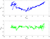 |
Fig. 5. Hodogram representation of the magnetic field components in the minimum variance reference frame: maximum-intermediate plane (blue line) and maximum-minimum plane (green line). |
The magnetic field hodogram representation highlights a clear rotation in maximum-intermediate plane, thus confirming the presence of an interplanetary magnetic FR (Moldwin et al. 2000).
In order to determine the main features of the FR, we also performed a Lundquist fitting procedure. The Lundquist FR model (Lundquist 1951) starts by solving the force-free equation J × B = 0. The force-free FR corresponds to the minimum energy state of FRs, in which the gradient of the thermal pressure is negligible (▿pth ∼ 0) and the magnetic pressure gradient is balanced by the magnetic tension force:
 (5)
(5)
Lundquist (1951) introduced the idea of using the Bessel functions to describe the force-free magnetic field lines in the cylindrical coordinates of FRs (see also Burlaga 1988)
 (6)
(6)
 (7)
(7)
 (8)
(8)
where BA is the axial magnetic field component, JB0 and JB1 are the zeroth and first-order Bessel functions, α = 2.4048 is a constant, B0 is the magnitude of the core field of the FR, BT is the tangential magnetic field component, H is the handedness of the magnetic helicity, and BR is the radial magnetic field component.
We have assumed a travelling speed of 340 km s−1 for the FR (according to the mean energy observed by SERENA/PICAM) and have deemed eint as the axial direction. The fitting curves are the coloured lines, which overlap with the grey, measured, magnetic field components in Fig. 6.
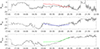 |
Fig. 6. Lundquist fitting results of the FR hitting BepiColombo: magnetic field components in the minimum variance directions (grey lines) superposed with fitting results (coloured lines). |
The fitting resulted in an impact parameter of 0.55, which indicated the closest approach distance to the centre of the FR to the radius of the FR. BepiColombo was approximately halfway from the centre of the FR. The fitting gave a radius of 2.1 × 10⁶ km and a core field of 19 nT for the FR.
As a final, further check to confirm our detection of the interplanetary FR, we performed a similar analysis (MVA and Lundquist fit) on Solar Orbiter (SolO, Müller et al. 2020) magnetic field data (Horbury et al. 2020). Indeed, SolO was located at a distance of 0.64 AU from the Sun (0.26 AU from BepiColombo) and the two spacecraft were radially aligned rather well, longitudinally separated by less than 10°, and lying on the same side of the heliospheric current sheet1. Figure 7 shows a comparison of the magnetic field intensity observed at the BepiColombo orbit and that observed at the SolO orbit, together with the cone and the clock angles observed at the SolO orbit.
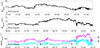 |
Fig. 7. Magnetic field intensity observed at the BepiColombo orbit (upper panel) and that observed at the SolO orbit (middle panel), together with the cone and the clock angles (lower panel) observed at the SolO orbit. |
As for BepiColombo, a clear rotation can be identified in SolO data lasting from 08:00 up to 09:15 where the clock angle describes an eastward-northward-eastward rotation. To better identify the FR, we again performed the MVA on Solar Orbiter data, whose results are shown in Table 2.
Eigenvalues λ and eigenvectors e of the covariance matrix C obtained from the Solar Orbiter magnetic field data.
Since the ratio between the eigenvalues is again larger than 3, then the minimum variance results are appropriately obtained. Figure 8 reports the hodogram representation of the magnetic field components in the minimum variance coordinate.
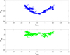 |
Fig. 8. Hodogram representation of the magnetic field components in the minimum variance reference frame: maximum-intermediate plane (blue line) and maximum-minimum plane (green line). |
A clear rotation of the magnetic field vectors is shown in the maximum-intermediate plane, which confirms the presence of an interplanetary magnetic FR.
As for BepiColombo, to determine the main features of the FR, we also performed a Lundquist fitting procedure (see Fig. 9). We have assumed a 340 km s−1 travelling speed of the FR as well. The impact parameter was determined to be 0.22, which indicated that Solar Orbiter traversed deeper into the core of the FR. The fitting resulted in a radius of 1.0 × 10⁷ km and a core field of 14 nT for the FR.
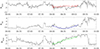 |
Fig. 9. Lundquist fitting results of the FR hitting Solar Orbiter: magnetic field components in the minimum variance directions (grey lines) superposed with fitting results (coloured lines). |
3.2. Interval (2) 20:34–20:44 and interval (3) 20:57–21:08: Low-energy ions
As shown in Fig. 2, PICAM observed low-energy wave-like signatures at the edges of the FR (marked by (2) and (3) in Fig. 2) which are rather well correlated with wave-like activities observed by MAG. To investigate the existence of waves, we performed a dynamical spectrum analysis on the magnetic field data rotated in the mean-field aligned (MFA) coordinate system. In this new system, the ZMFA is along the low-pass filtered magnetic field, while XMFA and YMFA are combined into a right- and left-handed coordinates:
 (9)
(9)
 (10)
(10)
The results for the compressional (C ≡ ZMFA) and the right- and left-hand polarized fields R/L are shown in Fig. 10.
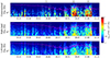 |
Fig. 10. Dynamical spectra of the compressional (C), right- (R), and left-hand polarized field components. The magenta line marks the proton cyclotron frequency fcp = 1.53 × 10⁻²|B|. The vertical dashed-dotted lines indicate the time intervals of interest marked by (1), (2), and (3), respectively. |
We clearly observed the enhancements in the power spectral density during intervals (2) and (3) at high frequencies, mostly centred around 0.1 Hz. More specifically, the compressional component of fluctuations, that is that aligned along the magnetic field, shows larger increases with respect to the right- and left-hand components. This suggests that there exist wave-like structures which locally accelerate low-energy ions observed by PICAM; on the other hand, the high-energy ion enhancements do not seem to be driven by wave-like processes. These wave-like structures can be the result of the passage of the interplanetary FR since they match its boundaries (edges). However, due to the low-resolution magnetic field data, we cannot explore if these wave-power enhancements can be attributed to specific patterns as whistler waves or the kinetic counterpart of Alfvénic correlated waves, that is kinetic Alfvén waves (KAWs), occurring at frequencies of tens of Hz. According to the range of frequencies, it seems they could be related to compressional waves likely generated by magnetohydrodynamic (MHD) ßinstabilities occurring around the ion cyclotron frequency, thus suggesting the possible occurrence of Kelvin–Helmholtz instability.
4. Conclusions
During its first flyby to Mercury on 01 October 2021, the SERENA/PICAM ion camera onboard BepiColombo observed both the background (thermal) solar wind distribution, mostly centred around 600 eV, thus corresponding to a slow solar wind, as well as the occurrence of high-energy (> -pagination1 keV) ion enhancements, mostly directed in the opposite direction to the solar wind plasma. By combining plasma and magnetic field measurements, we associated these intermittent features with the passage of a small interplanetary magnetic FR. Our findings have also been validated by means of Solar Orbiter measurements located at a larger distance (0.6 AU), also allowing us to retrieve the main features of the FR in its expanding phase. Furthermore, while the core of the FR produced high-energy (> -pagination1 keV) intermittent-like particle acceleration clearly distinct from the background solar wind (see interval (1) in Fig. 2), which is in agreement with previous observations and simulations (e.g., Zank et al. 2014; le Roux et al. 2015), at its edges compressional low-energy fluctuations have also been observed, likely generated by MHD instabilities occurring around the ion cyclotron frequency, thus suggesting the possible occurrence of Kelvin–Helmholtz instability (Van Eck et al. 2022). Summarizing, we reported the first case study of a magnetic FR simultaneously observed close to Mercury and further away, showing the potential of multi-spacecraft investigations for detecting solar transient events (Möstl et al. 2022). The detected FR (see a schematic view in Fig. 11) expanded its size from a radius of 2.1 × 10⁶ km at Mercury (0.4 AU) to a radius of 107 km at a Solar Orbiter location (0.6 AU). Its main core field reduced from 19 nT to 14 nT, thus suggesting that it continued to expand further away from Solar Orbiter. Indeed, according to the Parker field evolution B(r) = B0r−2, which represents a static view of the evolution of the interplanetary magnetic field, we should obtain a core field of ∼12 nT at a Solar Orbiter location. Furthermore, the two spacecraft crossed the magnetic FR in a different way: while BepiColombo observed a flux tube whose main axis was directed along the normal direction (i.e., perpendicular to the orbital plane of the spacecraft), the flux tube axis lies in the orbital plane at Solar Orbiter. Finally, according to preliminary analysis on the Hermean environment seen by BepiColombo (Orsini et al. 2022), the magnetosphere of Mercury was in its nominal conditions, thus suggesting that it reconfigured after the passage of the FR.
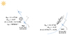 |
Fig. 11. Schematic view in the R − T plane of the evolution of the FR (size, direction, and parameters) from the BepiColombo to Solar Orbiter location. The FR rotated from the N direction into the R − T plane (see text for details). We note that RFR is radius of the FR, Bcore is core field of the FR, vFR is travel speed of the FR, and |

Acknowledgments
SERENA general management, SCU and ELENA are funded by the Italian Space Agency (ASI) and by the Italian National Institute of Astrophysics (INAF), agreement n. 2018-8-HH.0. SERENA ground-based activity is also funded by the European Space Agency (EXPRO contract). PICAM is funded mostly by the Austrian Space Applications Programme (ASAP) of the Austrian Research Promotion Agency (FFG), and partially by the Programme de Dévelopement d’Expériences (PRODEX), and by the CNES French Space Agency. The Solar Orbiter magnetometer was funded by the UK Space Agency (grant ST/T001062/1). D. Heyner was supported by the German Ministerium für Wirtschaft und Klimaschutz and the German Zentrum für Luft- und Raumfahrt under contract 50 QW1501.
References
- Akasofu, S.-I. 2021, Front. Astron. Space Sci., 7, 100 [NASA ADS] [CrossRef] [Google Scholar]
- Alberti, T., Laurenza, M., Consolini, G., et al. 2020, ApJ, 902, 84 [NASA ADS] [CrossRef] [Google Scholar]
- Benkhoff, J., Murakami, G., Baumjohann, W., et al. 2021, Space Sci. Rev., 217, 90 [NASA ADS] [CrossRef] [Google Scholar]
- Bothmer, V., & Daglis, I. A. 2007, Space Weather - Physics and Effects (Berlin/Heidelberg: Springer) [CrossRef] [Google Scholar]
- Burlaga, L. F. 1988, J. Geophys. Res. Space Phys., 93, 7217 [Google Scholar]
- Chen, C. H. K., Bale, S. D., Bonnell, J. W., et al. 2020, ApJS, 246, 53 [Google Scholar]
- Foullon, C., & Malandraki, O. 2018, in Space Weather of the Heliosphere: Processes and Forecasts (Cambridge: Cambridge University Press), IAU Symp. Proc., 335 [Google Scholar]
- Glassmeier, K. H., Auster, H. U., Heyner, D., et al. 2010, Planet Space Sci., 58, 287 [NASA ADS] [CrossRef] [Google Scholar]
- Gurnett, D. A., & Bhattacharjee, A. 2005, Introduction to Plasma Physics: with Space and Laboratory Applications (Cambridge: Cambridge University Press) [CrossRef] [Google Scholar]
- Heyner, D., Auster, H. U., Fornaçon, K. H., et al. 2021, Spcae Sci. Rev., 217, 52 [NASA ADS] [CrossRef] [Google Scholar]
- Horbury, T. S., O’Brien, H., Carrasco Blazquez, I., et al. 2020, A&A, 642, A9 [NASA ADS] [CrossRef] [EDP Sciences] [Google Scholar]
- le Roux, J. A., Zank, G. P., Webb, G. M., & Khabarova, O. 2015, ApJ, 801, 112 [Google Scholar]
- le Roux, J. A., Zank, G. P., & Khabarova, O. V. 2018, ApJ, 864, 158 [Google Scholar]
- Lundquist, S. 1951, Phys. Rev., 83, 307 [NASA ADS] [CrossRef] [Google Scholar]
- Mangano, V., Dósa, M., Fränz, M., et al. 2021, Spcae Sci. Rev., 217, 23 [NASA ADS] [CrossRef] [Google Scholar]
- Moldwin, M. B., Ford, S., Lepping, R., Slavin, J., & Szabo, A. 2000, Geophys. Rev. Lett., 27, 57 [NASA ADS] [CrossRef] [Google Scholar]
- Möstl, C., Weiss, A. J., Reiss, M. A., et al. 2022, ApJ, 924, L6 [CrossRef] [Google Scholar]
- Müller, D., St. Cyr, O. C., Zouganelis, I., et al. 2020, A&A, 64, A1 [CrossRef] [EDP Sciences] [Google Scholar]
- Orsini, S., Livi, S., Torkar, K., et al. 2010, Planet Space Sci., 58, 166 [NASA ADS] [CrossRef] [Google Scholar]
- Orsini, S., Livi, S. A., Lichtenegger, H., et al. 2021, Spcae Sci. Rev., 217, 11 [NASA ADS] [CrossRef] [Google Scholar]
- Orsini, S., Milillo, A., Lichtenegger, H., et al. 2022, Nat. Comm., 13, 7390 [NASA ADS] [CrossRef] [Google Scholar]
- Sarantos, M., Killen, R. M., & Kim, D. 2007, Planet Space Sci., 55, 1584 [NASA ADS] [CrossRef] [Google Scholar]
- Slavin, J. A., Acuña, M. H., Anderson, B. J., et al. 2009, Science, 324, 606 [NASA ADS] [CrossRef] [Google Scholar]
- Slavin, J. A., Imber, S. M., & Raines, J. M. 2021, in Magnetospheres in the Solar System, eds. R. Maggiolo, N. André, H. Hasegawa, & D. T. Welling, 2, 537 [NASA ADS] [Google Scholar]
- Sonnerup, B. U. O., & Cahill, L. J., Jr 1967, J. Geophys. Res. (1896–1977), 72, 171 [CrossRef] [Google Scholar]
- Sun, W., Dewey, R. M., Aizawa, S., et al. 2022, Sci. China Earth Sci., 65, 25 [NASA ADS] [CrossRef] [Google Scholar]
- Telloni, D., Sorriso-Valvo, L., Woodham, L. D., et al. 2021, ApJ, 912, L21 [NASA ADS] [CrossRef] [Google Scholar]
- Temmer, M. 2021, Liv. Rev. Sol. Phys., 18, 4 [NASA ADS] [CrossRef] [Google Scholar]
- Tu, C. Y., & Marsch, E. 1990, J. Geophys. Res., 95, 4337 [NASA ADS] [CrossRef] [Google Scholar]
- Van Eck, K., le Roux, J., Chen, Y., Zhao, L. L., & Thompson, N. 2022, ApJ, 933, 80 [NASA ADS] [CrossRef] [Google Scholar]
- Verscharen, D., Klein, K. G., & Maruca, B. A. 2019, Liv. Rev. Sol. Phys., 16, 5 [Google Scholar]
- Winslow, R. M., Anderson, B. J., Johnson, C. L., et al. 2013, J. Geophys. Res. (Space Phys.), 118, 2213 [NASA ADS] [CrossRef] [Google Scholar]
- Zank, G. P., le Roux, J. A., Webb, G. M., Dosch, A., & Khabarova, O. 2014, ApJ, 797, 28 [Google Scholar]
All Tables
Eigenvalues λ and eigenvectors e of the covariance matrix C obtained from the BepiColombo magnetic field data.
Eigenvalues λ and eigenvectors e of the covariance matrix C obtained from the Solar Orbiter magnetic field data.
All Figures
|
Fig. 1. Trajectory (dashed-dotted black line) of the first BepiColombo flyby to Mercury in the XMSO–ρMSO plane in units of the radius of Mercury, RM = 2439.7 km (the black arrow marks the spacecraft direction). The red line corresponds to the time interval considered in this study corresponding to PICAM measurements and when BepiColombo sampled the solar wind near Mercury. The grey line represents the average bow shock surface (Slavin et al. 2009; Winslow et al. 2013). The inbound and outbound bow shock crossings are marked by blue text. |
| In the text | |
|
Fig. 2. Omni-directional time–energy ion counts (top), magnetic field measurements (middle), and cone θc and clock ϕc angles (bottom). The vertical dashed-dotted lines indicate the time intervals of interest marked by (1), (2), and (3), respectively. The horizontal dotted line in the bottom panel refers to the Parker spiral angle θP, while the arrow marks the rotation of the magnetic field. |
| In the text | |
|
Fig. 3. High-energy (> 1 keV, top) and low-energy (< 1 keV, middle) ion counts in the solar wind direction (cyan lines) and in its opposite direction (magenta lines). Bottom: magnetic field measurements. The vertical dashed-dotted lines indicate the time intervals of interest (see Fig. 2). |
| In the text | |
|
Fig. 4. Behaviour of the magnetic field intensity B (black line) and the ratio between magnetic field fluctuations and its modulus δB/B (red line). The arrow marks the rotation of the magnetic field. |
| In the text | |
|
Fig. 5. Hodogram representation of the magnetic field components in the minimum variance reference frame: maximum-intermediate plane (blue line) and maximum-minimum plane (green line). |
| In the text | |
|
Fig. 6. Lundquist fitting results of the FR hitting BepiColombo: magnetic field components in the minimum variance directions (grey lines) superposed with fitting results (coloured lines). |
| In the text | |
|
Fig. 7. Magnetic field intensity observed at the BepiColombo orbit (upper panel) and that observed at the SolO orbit (middle panel), together with the cone and the clock angles (lower panel) observed at the SolO orbit. |
| In the text | |
|
Fig. 8. Hodogram representation of the magnetic field components in the minimum variance reference frame: maximum-intermediate plane (blue line) and maximum-minimum plane (green line). |
| In the text | |
|
Fig. 9. Lundquist fitting results of the FR hitting Solar Orbiter: magnetic field components in the minimum variance directions (grey lines) superposed with fitting results (coloured lines). |
| In the text | |
|
Fig. 10. Dynamical spectra of the compressional (C), right- (R), and left-hand polarized field components. The magenta line marks the proton cyclotron frequency fcp = 1.53 × 10⁻²|B|. The vertical dashed-dotted lines indicate the time intervals of interest marked by (1), (2), and (3), respectively. |
| In the text | |
|
Fig. 11. Schematic view in the R − T plane of the evolution of the FR (size, direction, and parameters) from the BepiColombo to Solar Orbiter location. The FR rotated from the N direction into the R − T plane (see text for details). We note that RFR is radius of the FR, Bcore is core field of the FR, vFR is travel speed of the FR, and |
| In the text | |
Current usage metrics show cumulative count of Article Views (full-text article views including HTML views, PDF and ePub downloads, according to the available data) and Abstracts Views on Vision4Press platform.
Data correspond to usage on the plateform after 2015. The current usage metrics is available 48-96 hours after online publication and is updated daily on week days.
Initial download of the metrics may take a while.