| Issue |
A&A
Volume 698, June 2025
|
|
|---|---|---|
| Article Number | A12 | |
| Number of page(s) | 11 | |
| Section | Planets, planetary systems, and small bodies | |
| DOI | https://doi.org/10.1051/0004-6361/202453452 | |
| Published online | 03 June 2025 | |
Hybrid modeling of Mercury’s magnetosphere: Assessing accuracy in ion counting statistics
1
Space Research Institute Graz, Austrian Academy of Sciences,
Graz,
Austria
2
Institute of Physics/IGAM, University of Graz,
Graz,
Austria
3
European Space Agency, ESTEC,
Noordwijk,
The Netherlands
4
Institute of Geophysics and Extraterrestrial Physics, Technische Universität Braunschweig,
Braunschweig,
Germany
5
Institute of Theoretical Physics, Technische Universität Braunschweig,
Braunschweig,
Germany
6
Graduate School of Science, Data Analysis Center for Geomagnetism and Space Magnetism, Kyoto University,
Kyoto,
Japan
7
INAF-IAPS,
Rome,
Italy
★ Corresponding author: This email address is being protected from spambots. You need JavaScript enabled to view it.
Received:
15
December
2024
Accepted:
3
April
2025
Abstract
In this study, we present a method for comparing hybrid plasma simulations with spacecraft measurement data, with a focus on Mercury’s interaction with the solar wind. Utilizing the 3D global hybrid simulation model Adaptive Ion-Kinetic Electron-Fluid (AIKEF), we derived ion energy distributions in Mercury’s magnetosheath using different solar wind input scenarios. We introduce three concepts for counting the simulated particles and assess the systematic and stochastic variations. Furthermore, we evaluate the effect of different phase space resolutions within the model. We find that a lower phase space resolution influences the distribution peaks, thus emphasizing the need for adequate particle resolution. Dedicated simulation runs for BepiColombo’s second and third flyby maneuvers at Mercury, based on solar wind measurement data from the BepiColombo fluxgate magnetometer on board the Mio spacecraft (Mio-MGF) and Planetary Ion Camera (PICAM) instruments, enable quantitative comparison of simulated data with ion spectrometer measurements. The energy flux distributions measured by PICAM fall within the confidence intervals of the modeled data. Additionally, we find that systematic deviations dominate the stochastic deviations. Our analysis shows that our simulation is an effective tool for understanding magnetospheric conditions, and it can assist in interpreting the in situ spacecraft measurements from BepiColombo upon its arrival.
Key words: plasmas / instrumentation: miscellaneous / methods: numerical / solar wind / planets and satellites: magnetic fields / planet–star interactions
© The Authors 2025
 Open Access article, published by EDP Sciences, under the terms of the Creative Commons Attribution License (https://creativecommons.org/licenses/by/4.0), which permits unrestricted use, distribution, and reproduction in any medium, provided the original work is properly cited.
This article is published in open access under the Subscribe to Open model. This email address is being protected from spambots. You need JavaScript enabled to view it. to support open access publication.
1 Introduction
In the past decades, numerical approaches to modeling the behavior of space plasmas have become increasingly prevalent. Advances in computational power have made it possible to run simulations that are considerably more complex than those achievable in the past within reasonable time frames. However, as computational resources remain limited, trade-offs still need to be made. Hence, the choice of a plasma model depends highly on the type of application. At large scales, a plasma can be well described by a fluid magnetohydrodynamic (MHD) approach. Nevertheless, in certain situations the kinetic description of particles becomes essential, such as when studying turbulence and wave-particle-interactions, particle acceleration, or non-Maxwellian velocity distributions. In these cases, the individual motion of charged particles and their interactions cannot be adequately captured by the macroscopic approach of MHD. Particle-in-cell (PIC) models solve the equation of motion for every particle individually at each given time step. Similar to most MHD models, the electromagnetic fields are calculated on discrete nodes of a pre-defined mesh grid. As the kinetic time and length scales of electrons is much smaller than for protons (and heavier ions) due to the mass difference of mp = 1836 me, the time step in the model needs to be adequately small to resolve electron gyrations properly, for example. While PIC models have been used to study phenomena on electron kinetic scales using confined simulation boxes, they result in a huge computational effort when trying to model the global interaction of a planet with the solar wind. For such cases, hybrid models are often used as a computational compromise (Trávníček et al. 2007, 2009; Paral et al. 2010; Paral & Rankin 2013; Müller et al. 2011; Müller et al. 2012; Herčík et al. 2013; Fatemi et al. 2017, 2018, 2024; Exner et al. 2020, 2024; Jarvinen et al. 2020; Aizawa et al. 2021; Lu et al. 2022). In these models, ions are treated kinetically, whereas electrons are treated as a fluid and are not resolved in velocity space (Winske & Omidi 1996).
While Mercury’s magnetosphere is similar to Earth’s, it is much smaller and more dynamic due to stronger solar wind pressure, which is five times higher, and a weaker planetary magnetic field (Winslow et al. 2013). The Dungey cycle at Mercury takes only about two minutes, compared to one hour at Earth, indicating a faster response to solar wind changes (Slavin et al. 2009; Slavin et al. 2021; Sun et al. 2022). Unique features such as the absence of a significant ionosphere and the presence of a large conducting core strongly influence Mercury’s magnetospheric currents and induction effects (Smith et al. 2012; Jia et al. 2015; Exner et al. 2020). The ESA/JAXA BepiColombo mission (Benkhoff et al. 2010, 2021) was launched in October 2018 and will conduct a total of six Mercury fly-bys before entering its final science orbit around the planet in 2026. Although the primary science phase starts after the spacecraft reaches its final orbit, the flybys offer valuable scientific opportunities by crossing Mercury’s magnetosphere at various angles. During these maneuvers, the spacecraft will approach as close as 165 km and provide unique insights into the global magnetosphere.
A complex scenario, such as the interaction of a planet with its host star, can be modeled using numerical simulations. However, the underlying simplified models and their implementation introduce errors or deviations from the real-world scenario. The following two paragraphs summarize the main sources of deviations introduced by numerical models in two categories, systematic and stochastic deviations.
Systematic deviations arise from the fundamental limitations of numerically approximating continuous physical systems. Currently, most of nature is understood to be continuous (classical mechanics, electromagnetism, and fluid dynamics), which is something that cannot be numerically represented with absolute accuracy. To cope with this issue, numerical models need to be discretized, for instance in space and time (Winske & Omidi 1996). While these discretization processes are designed to be consistent and repeatable, they inherently introduce various errors. Time integration, for instance, can be done using first-order techniques such as the Euler method, which calculates the next state of a system based on its current state, using a discrete time step. This method potentially introduces an increasing systematic error no matter how small the chosen discrete time step. More sophisticated higher-order models such as the Runge–Kutta algorithms offer improvements regarding this issue but are still not exact (Driscoll & Braun 2022). A similar error is introduced by numerical algorithms to solve ordinary and partial differential equations, which often occur in fluid dynamics (Schulz et al. 2011). Moreover, the selection of the spatial resolution (i.e., grid size) can introduce numerical artifacts or lead to errors, especially if the grid spacing is not fine enough to adequately resolve the occurring physical processes. Other aspects are the limited simulation box size and the defined boundary conditions. Both conditions can greatly affect the simulation outcome and need to be chosen carefully. Furthermore, choices made during model development for simplification or efficiency or both (such as using a hybrid approach, macro-particles, smoothing or numerical diffusion techniques, etc.) consistently impact the accuracy of simulations (Shadwick et al. 2014; Lapenta et al. 2022). The use of macro or super particles, for instance, reduces the computational effort but affects the resolution in phase space, and a low macro-particle count causes statistical noise (Bagdonat & Motschmann 2002). Last but not least, inaccuracies or uncertainties in model (input) parameters introduce systematic deviations of a simulation outcome and real measurements.
Stochastic deviations, on the other hand, originate from inherent uncertainties and probabilistic elements within the modeling framework. Stochastic factors refer to sources of randomness or uncertainty that can introduce variability in the simulation results. Similar to what has already been mentioned about the systematic deviations, model simplifications can introduce stochastic errors (e.g., by not fully capturing the complexity of reality and stochastic processes, such as turbulence (Bourgoin & Xu 2014)). In general, simulating random processes, such as particle motion in a fluid, introduces stochastic deviations natural to the modeling process. Furthermore, numerical methods used in simulation models inherently involve randomness or noise, such as round-off errors caused by the finite precision of computational systems.
Important to note is that deviations such as scale discrepancies can be both systematic and stochastic. While physical phenomena often occur across multiple scales, such as energy transfer from fluid to kinetic scales in space plasma physics (Kiyani et al. 2015), simulations can suffer from limitations in resolving multi-scale interactions, which can lead to deterministic and stochastic discrepancies.
While there are many hurdles to overcome, numerical modeling efforts have added invaluable insights to understanding nature and have also become essential in engineering (e.g., Rao (2010)). Various techniques and methods have been developed to overcome error propagation and improve models. The most important task is model validation against measurement data. This iterative process involves running simulations, comparing the results to measurements, and refining the model accordingly. Complex planet-star interactions have been successfully modeled in this way in the sense of delivering representative results compared to measurements. A few examples for the global hybrid modeling of the Sun-Mercury interaction have already been mentioned, but PIC (e.g., Lavorenti et al. 2022) and MHD approaches (e.g., Aizawa et al. 2018; Jia et al. 2019; Griton et al. 2023; Varela & Pantellini 2023) have also been used to model Mercury’s plasma environment. Numerical models have likewise been applied to study the solar wind interaction with other planets, including Mars (e.g., Jarvinen et al. 2018; Fang et al. 2017), Venus (e.g., Aizawa et al. 2022), and Earth (e.g., Palmroth et al. 2018).
In this work, the hybrid model Adaptive Ion-Kinetic Electron-Fluid (AIKEF; Müller et al. (2011)) is used to model the interaction of the planet Mercury with the solar wind. The kinetic description of the ions allows us to use the modeled particle data to perform a statistical analysis, which is the focus of this work. Our goal is to assess systematic and stochastic deviations and confidence intervals of “ion counting” in the hybrid model. The purpose is not to validate the hybrid model itself (hybrid models can be applied to model Mercury’s magnetosphere with limitations compared to including electron kinetic effects; see Lapenta et al. (2022)) but rather to establish a method to evaluate the accuracy of a given quasi-stationary simulation output. For this, three approaches, a simple “sphere counting” (Teubenbacher et al. 2024), “omnidirectional counting” and a “field-of-view” (FOV) method are introduced. The resulting ion velocity distribution functions are then compared to measurements of the Planetary Ion CAMera (PICAM; Orsini et al. (2010, 2021)), which is an ion mass spectrometer on board the Mercury Planetary Orbiter (MPO) spacecraft of the BepiColombo mission. The measurements used for comparison in this work were taken during the magnetosheath crossing of the second and third Mercury flybys of BepiColombo (henceforth MSB2 and MSB3, for Mercury SwingBy) on 23 June 2022 and 19 June 2023.
2 Methodology
During the planetary flybys, most of the scientific instruments on BepiColombo are activated. However, because the three Bepi-Colombo spacecraft are in a stacked configuration during the cruise phase (Benkhoff et al. 2010, 2021), some instruments have a restricted FOV, and most are still being commissioned. In this context, we utilized four-second spin-averaged magnetic field data (L-mode) from the Mio fluxgate magnetometer (Mio-MGF; Baumjohann et al. 2020). It is important to acknowledge that the MGF magnetometer mast remains in its stowed configuration, with the sensor housed within the spacecraft canister. Consequently, this positioning introduces potential uncertainties in the measurements due to possible interferences originating from the spacecraft itself. For MSB2, the chosen time frame to evaluate the interplanetary magnetic field (IMF) input for the simulation (see Table 1) is taken after the outbound bow shock crossing from 2022-06-23 10:05:00 to 10:15:00 UTC. This time frame was used to exclude possible foreshock wave observations. The time frame for MSB3 was taken on the inbound bow shock crossing from 2023-06-19 18:33:40 to 18:43:40 UTC. The IMF vectors given in Table 1 have an uncertainty of ± 7 nT.
The upstream solar wind densities and velocities used as simulation input in this study (see Table 1) were estimated based on PICAM measurements obtained under upstream conditions following the MSB2 and MSB3 events, as provided by the instrument team. PICAM is an all-sky camera for ions that allows for the determination of the velocity distribution and mass spectrum of ions over an instantaneous hemispheric field of view, from thermal up to ∼3 keV energies and in a mass range extending up to ∼132 amu and with a mass resolution better than ∼50 (Orsini et al. 2010, 2021). While PICAM is not specifically designed or optimally positioned for solar wind observations (being instead configured to maximize the detection of planetary ions), it is nevertheless capable of detecting solar wind ions. The solar wind speed is estimated by converting the peak energy of the measured distribution, assuming a proton mass and using the relation E = 0.5mv2. Determining the density, however, is significantly more challenging, as the core solar wind population lies outside PICAM’s field of view, thus only allowing for a broad range estimation rather than an exact value. Nevertheless, based on PICAM measurements, we derived a probable density estimate required for our analysis, which was further validated through test simulations with varying density values. The uncertainty in the solar wind speed is derived from the instrumental energy resolution and its associated error, which depends on the operational mode of PICAM. For MSB3, for instance, the estimated uncertainty in velocity is approximately 7%, corresponding to an uncertainty of 25 kms/s.
The PICAM time frames are 2022-06-23 09:52–09:53 UTC for MSB2 and 2023-06-19 19:48–19:51 UTC for MSB3. Although the solar panels of the transfer module in the stacked spacecraft configuration can generally cause FOV obstructions, in our specific cases and pointing configurations during MSB2 and MSB3, the FOV remains unobstructed. During these time windows, PICAM operated in image mode 4 with an effective accumulation time of ΔtPICAM = 219 ms (nominal 219 ms, minus 31 ms settling time). The chosen time windows are representative samples from the magnetosheath during MSB2 and MSB3.
The AIKEF code was used to model a global quasi-stationary 3D picture of Mercury’s magnetosphere. The model treats ions kinetically and electrons as massless charge-neutralizing fluid. A detailed explanation of the model and its implementation can be found in Müller et al. (2011). Table 1 summarizes the key simulation setup and physical input parameters for five chosen scenarios.
The scenarios S1, S2, and S3 assume an “open magnetosphere” (Vernisse et al. 2018; Aizawa et al. 2021; Jia et al. 2019; Trávníček et al. 2010; Fatemi et al. 2024), meaning a completely southward IMF, with an average magnitude derived from MESSENGER (Solomon et al. 2007) measurement studies by James et al. (2017). While S2 uses mean upstream solar wind conditions, S1 and S3 are the lower and upper boundary of the expected upstream solar wind velocity, density, and temperature based on a statistical solar wind study by Dakeyo et al. (2022). The resulting varying Alfvénic Mach numbers (see Table 1) affect the formation of the bow shock wave. We note that Lai et al. (2024) have shown that the bow shock disappears for very low Mach numbers (MA ≤1.5); however, this is not the case for our study, as the lowest Mach number is MA = 3.9 for the MSB3 scenario (see Table 1). The solar wind input parameters of the MSB2 and MSB3 scenarios are adjusted to particle measurement values of PICAM (Orsini et al. 2010, 2021) and Mio MGF (Baumjohann et al. 2020) measurements during the outbound trajectory phase in order to obtain the IMF direction and strength.
In the model, the planetary magnetic field is considered up to the octopole moment (Anderson et al. 2012; Exner et al. 2024), and the planet itself is a spherical object of Mercury’s radius RM = 2440 km that absorbs incoming particles. Furthermore, we limited our study to one ion species, namely, protons of solar wind origin, as they are one of the dominant species, alongside alpha particles (He2+) and heavier ions. These ions are modeled using a macro-particle approach, where the optimal number of macro-particles per mesh grid cell (oMPIC) is an input parameter that affects the resolution of the velocity distribution and further the computational time. More precisely, the more macroparticles per cell that are used, the fewer “physical” particles that need to be coalesced, thus increasing the phase space accuracy but at the cost of a higher computational demand. To evaluate the effect of changing this parameter, we repeated the three scenarios described in Table 1 for oMPIC = 3 and oMPIC = 15, respectively. The BepiColombo MSB2 and MSB3 scenarios were run with oMPIC = 50 to better resolve the phase space for direct comparison to measurements with the cost of a significantly longer computational time. Particle splitting and merging procedures were used (as described in Müller et al. (2011) mass, momentum and kinetic energy were conserved) to ensure the same number of macro-particles per cell throughout every cell of the mesh grid. However, the actual number of macro-particles in each cell (MPIC) varies depending on how strong and often the splitting and merging is applied. For the oMPIC = 3 scenario, strong merging was applied to ensure MPIC ∼ 3 and show the effect of strong particle noise. In the oMPIC = 15 and oMPIC = 50 cases, the merging was applied less strongly, which naturally results in a higher MPIC count in cells where the plasma density is high, such as in the magnetosheath (MPIC ≳ 3 oMPIC). The model uses the right-handed Mercury Anti Solar Orbital (MASO) coordinate system, where the x-axis is directed parallel to the solar wind velocity, the z-axis is the positive normal to the orbital plane (anti-parallel to Mercury’s dipole moment), and the y-axis is the orthogonal complement pointing roughly toward Mercury’s orbital movement direction.
In this study, we focus on the magnetosheath because it is characterized by high temperatures and dense plasma, making it an ideal region for conducting comparative analyses between observational and modeled data. The selected area is shown in Fig. 1 together with the MSB2 and MSB3 flyby trajectories and PICAM measurement time periods. The PICAM time frames are 2022-06-23 09:52–09:53 UTC for MSB2 and 2023-06-19 19:48–19:51 UTC for MSB3. The particle phase space data (i.e., positions and velocity vectors) were extracted from the simulation after about three to five solar wind box crossings, when quasi-stationarity was reached. The simulation box is centered at the planetary origin, measures 10 RM × 10 RM × 10 RM, and includes a refined region with enhanced mesh resolution by a factor of two near the planet (∼3 RM in each direction around the planet, covering the magnetosheath target area). To evaluate the stochastic deviation, the particle data were saved every 0.2 sec for 100 times, resulting in a time frame of about 20 sec of simulation time. While this represents about 10% of the total simulation time, it covers the solar wind passing from the subsolar point to about XMASO = 2 RM once. Given that the simulation assumes a steady and uniform solar wind input, this time frame corresponds to the transit time of solar wind particles through the magnetosheath. This provides a basis for assuming that the key interaction dynamics, including stochastic deviations, are addressed within a timescale relevant to the plasma flow regime.
Before calculating the velocity distributions, three different approaches were chosen to filter the particle data. Firstly, to get a qualitative overview of the plasma environment, an energy distribution was derived from particles within a sphere volume centered at consecutive trajectory points regardless of their movement direction (Teubenbacher et al. 2024); an illustration is shown in Fig. 2a. The radius of the sphere was chosen to be rsphere = 10 di,sw. This method gives a qualitative insight into the plasma environment of the given location. However, it might lead to results that cannot be directly compared to measurements of a particle instrument, as particles far from (maximum distance is rsphere) the observation region are counted equally as particles that are closer.
The second method employs a different approach that gets one step closer to how an actual instrument would measure (omnidirectional) particle flux (see Fig. 2b). First, an energy range is defined, for example Emin = 10 eV and Emax = 10 keV, and then divided into 30 logarithmic energy bins Ei. Then, if an integration time of Δt = 1 s (≈ 4 · ΔtPICAM) is assumed, the energy bins can be converted into “distance bins” at distances  . As only particle energies up to 10 keV are considered, we neglected relativistic effects that only become significant when the particle’s speed approaches a considerable fraction of the speed of light (10 keV protons have a speed of 1385 km/s, compared to the speed of light c ≈ 3·106 km/s). Particle counting is performed by selecting particles that fall within each bin, both in terms of spatial location and energy. Spatially, each bin corresponds to a outer sphere with a volume of
  . Additionally, particles must have an energy within the limits defined by the corresponding energy bin. For example, a particle with a distance to the spacecraft d∗ and energy E∗ has to fulfill d∗ ≤d3 and E2 < E∗ ≤E3 in order to be counted in the second bin. There is no inner distance boundary for particles, meaning higher energy particles can be located closer to the simulated detector than the inner edge of a given distance bin as long as they arrive within the accumulation time window. The energy window acts as a filter to prevent double counting of low energy particles in overlapping bins, which would otherwise lead to an artificially high contribution from lower energy bins. Next, the particles were filtered so that the tangential distance of each velocity vector to the spacecraft does not exceed a certain artificial spacecraft boundary with radius rsat = 100 km (for the high resolution phase space case and rsat = 200 km for the low resolution case). This parameter is used as a criterion to select only particles moving toward the spacecraft and indirectly creates a margin on the incidence angle. The maximum angular margin δ within which a particle is considered to be moving toward the detector, based on the particle’s position relative to the satellite, is dependent on rsat and the distance of the particle to the satellite rparticle and given by δ = tan−1(rsat/rparticle). A realistic radius rsat similar to the spacecraft or detector scale size is not possible due to the computationally limited phase space resolution. However, if rsat is too large, it averages over broader spatial regions, potentially smoothing out localized kinetic effects. To resolve kinetic effects, rsat should remain smaller than the characteristic length scales of relevant plasma structures. In this case, the maximum value for rsat corresponds to the magnetosheath thickness. After applying these filters, the number of particles in each bin Ni is given by
 (1)
with Ji being the total number of particles that fulfill the criteria mentioned above. The weight factor w′j for each (macro-) particle is used to renormalize to the physical number of particles. Within the AIKEF model, the simulation uses a normalized weight factor wj obtained using normalized and dimensionless values for the plasma number density and cell volume. As an example of renormalization, we computed the weight factor w′ of a macro-particle initialized as solar wind in scenario S1 with Vcell = (24 km)3, n0 = 80 cm−3, and oMPIC = 50:
(1)
with Ji being the total number of particles that fulfill the criteria mentioned above. The weight factor w′j for each (macro-) particle is used to renormalize to the physical number of particles. Within the AIKEF model, the simulation uses a normalized weight factor wj obtained using normalized and dimensionless values for the plasma number density and cell volume. As an example of renormalization, we computed the weight factor w′ of a macro-particle initialized as solar wind in scenario S1 with Vcell = (24 km)3, n0 = 80 cm−3, and oMPIC = 50:
 (2)
(2)
This equation indicates that each macro-particle in this “solar wind cell” represents a particle cloud of 2.21·1019 physical particles. If the physical number density changes, the aforementioned splitting and merging procedures try to preserve the given oMPIC value.
The width of each bin i, given in eV, is ΔEi = Ei+1 − Ei. Due to the logarithmic stepping, the bin width scales proportionally with energy; that is, ΔEi ∝ Ei. This logarithmic energy binning inherently accounts for the increasing bin volume at higher energies, and normalization by ΔEi ensures a consistent flux calculation across all energy bins.
Finally, the differential number flux  for each energy bin i given in #/(s eV cm2 sr) is formulated as
 (3)
where the solid angle Ωomni = 4π sr and the area
(3)
where the solid angle Ωomni = 4π sr and the area  in square centimeters are used to normalize in this omnidirectional scenario. Combining the fluxes ϕi from the individual energy bins results in a differential number flux profile, thus allowing one to analyze how particle flux varies with energy across the specified range. If we then multiply the number of particles by their energy Ej, we get the differential energy flux
  that is then used to compare the simulation data to measurements:
 (4)
(4)
As a third iteration, we introduce the FOV approach (see Fig. 2, panel c), where particles are counted in a manner similar to the omnidirectional approach, but we additionally introduce a cone angle that limits the direction of incoming particles and mimics the opening slit (or FOV) of the particle instrument. This FOV cone opening angle γ determines the maximum angle of the incident particles with respect to the cone direction. The normalization parameter  is adapted to the area of the cone section of the sphere, with rsat determined as described in the omnidirectional method. For the cone angle, the average effective acceptance angle of the PICAM instrument γ = 120° is used, and the solid angle Ω is also adapted (Ω120° = π sr). The incidence angle is geometrically limited by the margin δ, and additionally we set a maximum to γ/2 = 60° to exclude particles with high incidence angles that contribute less (incidence angle above 60° means less than 50% flux) to the flux compared to particles with velocity vectors (quasi-)parallel to the detector normal. The FOV cone orientation was chosen to match the boresight pointing of PICAM during the flybys and is in the +Z direction (or in polar and azimuthal angles in spherical coordinates: θ = 0°, ϕ = 0°) for MSB2 (and also S1, S2 and S3 scenarios) and in the north dawn direction (θ = 30°, ϕ = 30°) for the MSB3 scenario (ESA SPICE Service 2024).
Subsequently, we computed the energy distributions using each of the three techniques introduced above. A velocity histogram with logarithmi bin sizes was computed. The number of bins was chosen to be  , where N is the maximum number of particles in the 100 realizations. For each velocity bin, we defined a confidence interval using Student’s t-distribution, which is preferred over the normal distribution due to the relatively small sample size (the largest sample size is less than 500) and the unknown standard deviation of the population. The t-distribution provides intervals that are more conservative, thus accounting for additional uncertainty in the sample. The confidence interval, CI, can be calculated as
 (5)
where
(5)
where  is the sample mean of realization i, si is the sample standard deviation, n = N − 1 denotes the degree of freedom, α = 0.05 is chosen to give a 100(1 − α)% = 95% confidence, and tn;α/2 = t99;0.025 ≈ 1.984 is the percentage point of the t distribution.
Main input parameters used in the AIKEF model.
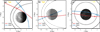 |
Fig. 1 Trajectories and target magnetosheath interval. Panel a shows the top view (xy-plane), panel b shows the side view from the dawnside (xz-plane), and panel c shows the view from the back (yz-plane). MASO coordinates are used. The BepiColombo MSB2 and MSB3 trajectories are respectively shown with a solid red and solid blue line, and the PICAM measurement time frames are indicated in rectangles. Models for the magnetopause and bow shock are illustrated by the black dashed (Winslow et al. 2013) and black solid (Slavin et al. 2009; Winslow et al. 2013) lines at X, Y, Z = 0, respectively. |
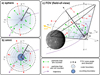 |
Fig. 2 Field-of-view particle counting schemata. Panel a shows the sphere method, panel b shows the omnidirectional method, and panel c shows the FOV method. The purple line shows an arbitrary spacecraft trajectory, rsat is the base circle to count incident particles, γ is the cone opening angle, and dmax is the maximum counting distance from the base circle. The dots show example particles with their velocity vectors. While the green particles were counted, the red ones were neglected, as (1) they are located outside the cone or their distance to the base circle is larger than dmax, (2) they are inside the cone but do not intersect the base circle, or (3) they are inside the cone pointing toward the base circle, but their energy and distance do not correspond to the criterion mentioned in the text. The coordinates are given in MASO (explained in the text) shifted to the center of each trajectory point. |
3 Results and interpretation
In total, eight simulation runs were performed. We ran a minimum, an average, and a maximum solar wind input scenario with a southward IMF each for two different input settings of the phase space resolution parameter oMPIC = 5 and oMPIC = 15. Additionally, we conducted two runs tailored to the MSB2 and MSB3 solar wind upstream conditions with a higher oMPIC (see Table 1). Due to the different solar wind speeds, quasistationarity was reached after a varying number of simulation time steps. Adapting to the slowest solar wind speed of 250 km/s, all simulations ran for about 220 s, which is approximately two Dungey cycles (Slavin et al. 2009), to become quasi-stationary. At this point, the simulations were continued for about 22 s, during which 100 realizations were saved continuously (every 1/5 sec) for each scenario. The magnetosheath particle distributions shown in Figs. 4 and 5 are derived from regions centered on the PICAM magnetosheath observation time windows (indicated by white crosses in Fig. 3).
The results for the location of the magnetospheric boundaries are shown in Fig. 3. The boundaries are derived from ion density and electric current  structures. The stand-off distances (shown at ZMASO = −0.3 RM for MSB2 and ZMASO = 0 RM for MSB3) largely depend on the solar wind ram pressure and Alfvénic Mach number (Winslow et al. 2013). As expected, the higher the ram pressure and Alfvénic Mach number, the thinner and closer to the planet is the magnetosheath. Moreover, due to the very small and slightly northward IMF direction during MSB2, the foreshock region is located at the dawnside at almost exactly the MSB2 outbound bow shock crossing (Fig. 3c). This has an effect on the general shape of the bow shock boundary (Teubenbacher et al. 2024). The black solid lines in all panels represent the average bow shock and magnetopause boundaries from Winslow et al. (2013). For the magnetopause, they use a power-law relationship between the focal parameter p and the Alfvénic Mach number
  . They also use a power law to fit the bow shock:
 ![Mathematical equation: ${R_{ss}} = (2.15 \pm 0.1) \cdot P_{{\rm{ram\;}}}^{[( - 1/6.75) \pm 0.024]}$](/articles/aa/full_html/2025/06/aa53452-24/aa53452-24-eq16.png) , where Rss is the subsolar bow shock stand-off distance and Pram is the solar wind ram pressure. The solid black lines for these boundaries in Fig. 3 were then computed using these empirical power laws and our model input values for Pram and MA (see Table 1; the MSB2 scenario parameters in panels a and c and MSB3 parameters in b and d). As these models are symmetric about the x-axis, the functions are rotated and sliced at ZMASO = −0.3 RM for MSB2, and ZMASO = 0 RM for MSB3 to better compare it with the modeled data.
, where Rss is the subsolar bow shock stand-off distance and Pram is the solar wind ram pressure. The solid black lines for these boundaries in Fig. 3 were then computed using these empirical power laws and our model input values for Pram and MA (see Table 1; the MSB2 scenario parameters in panels a and c and MSB3 parameters in b and d). As these models are symmetric about the x-axis, the functions are rotated and sliced at ZMASO = −0.3 RM for MSB2, and ZMASO = 0 RM for MSB3 to better compare it with the modeled data.
While the PICAM time windows are located in the magnetosheath right after crossing the “Winslow magnetopause,” the same time windows are located just within the modeled bow shock boundaries for both MSB2 and MSB3 (Figs. 3c and d). In general, the boundaries from Winslow et al. (2013), especially the bow shock, are farther away from the planet than the modeled data. However, it is important to mention that the focal parameter p, for instance, has large error margins that result in possible bow shock stand-off distances that would also include our modeled data (with MA = 3.9: (1.3 < p < 6.7); hence, the subsolar bow shock stand-off distance has a wide range: 1.17 RM < Rss,bs < 3.9 RM. The simulated magnetopause is also located closer to the planet, which is consistent with other hybrid simulations by Fatemi et al. (2018). In that study, the authors also derived a power law for the magnetopause boundary depending on MA, which is plotted as a dash-dotted line in Fig. 3. It is important to note that this power law is derived from simulations with solar wind ram pressures less than 10 nPa, which might not be valid for scenarios with large ram pressures such as S3 or MSB3. Nevertheless, the general shape and stand-off distances of the magnetopause reported by Fatemi et al. (2018) align more closely with our modeled data compared to those derived from the average parameters in Winslow et al. (2013), see in Fig. 3 panels b and d). However, our findings remain within the lower limit of the empirical range reported by Winslow et al. (2013). In their study, they evaluated the fitting parameters by binning the ram pressure, and the mean of the largest bin was 24 nPa, which is slightly lower than the value in our MBS3 case (Pram = 27.4 nPa). Furthermore, our results are consistent with studies of extreme solar wind conditions presented in Slavin et al. (2014) and compared in Fatemi et al. (2018).
In Fig. 4, we present our modeled energy distributions for oMPIC = 3 (left column) and oMPIC = 15 (right column). Our three counting methods are depicted in the rows. The solid lines represent the respective sample means at each energy bin, and the shaded area represents the 95% confidence interval. While the vertical dashed lines represent the mean energy of the solar wind inputs, the solid vertical lines show the maxima of each magnetosheath distribution. Figure 4 c is empty, as the phase space resolution of oMPIC = 3 is too low to determine an FOV spectrum. No particles fulfill the filtering criteria of the FOV approach, and therefore no flux could be calculated.
In case S3 (maximum solar wind input) the (virtual) spacecraft is located outside the bow shock in the solar wind. This means that the flux in red in panels b and e in Fig. 4 peaking at 1.58 keV would have been sampled from the solar wind instead of the magnetosheath (in reality, the solar wind is shocked at the bow shock and not measured from within the magnetosheath). Panels a and d show a similar feature; however, in this simple sphere approach we see both the magnetosheath and solar wind particle populations. Although the distribution of S3 (red) is broad and has flux in all energy bins in panel a (oMPIC = 3), panel d (oMPIC = 15) shows a peak flux just below the solar wind speed at around 1.45 keV. Nonetheless, a superposition of another particle population, characterized by its broad (hot) distribution, can be seen peaking above 500 eV in panel d. This population corresponds to the magnetosheath flux, with the sudden increase in flux at around 400–500 eV separating the two populations. This is evident in Fig. 3c, where the gray circle representing the energy bin covering solar wind-speed protons extends across both the magnetosheath and solar wind regions. In the omnidirectional method shown in panels b and e, applying the FOV approach to S3 leads to no flux (Fig. 4f) due to the northward pointing and the position in the solar wind instead of the magnetosheath.
In the average solar wind case (S2), the simple sphere method leads to broad fluxes in both phase space resolution scenarios, displayed in green in panels a and d. At oMPIC = 3, the peak is around 600 eV, and at oMPIC = 15, the peak is around 760 eV, just below the solar wind peak energy of S2 at 835 eV. This again means that the flux is an apparent combination of both particle populations, solar wind, and magnetosheath, which is also evident from the spatial location of MSB2 bordering the bow shock of scenario 2 in Fig. 3a and confirmed by the synthetic distributions in Fig. 5b. Moreover, panel b shows both populations with peaks at 710 eV (solar) and 300 eV (magnetosheath). Interestingly, the “solar wind peak” disappears in panel e (green line) when using the omnidirectional approach. Here, only one peak at 600 eV can be seen that belongs to the magnetosheath. Filtering the data even further using the FOV approach leads to a magnetosheath peak energy of 410 eV.
For the minimum solar wind case (S1) in Fig. 4, plotted in yellow, the shape of the distributions using the sphere method is similar to the S2 scenario (see panels a and d). The main differences are the lower peak energies at about 125 eV (oMPIC = 3) and 250 eV (oMPIC = 15) compared to the S2 case. Figure 4b shows flux for S2 only in a very limited energy range as a result of low count rates. Nevertheless, the peak energy can be identified at around 230 eV. Using a higher phase space resolution (panel e, oMPIC = 15) leads to a peak at 195 eV, and with enhanced resolution, the flanks of the distribution can also be calculated. When comparing the peak energies (vertical solid lines) in Fig. 4, panels e and f, while S1 stays at the same bin, there is a shift of around 200 eV to lower energies for the S2 scenario. In the omnidirectional approach, more particles from the solar wind are counted, which are out of view in the (northward) FOV used to create panel f.
Compared to the systematic errors introduced, the stochastic deviations play a minor role. Based on Fig. 4e, the stochastic error, represented by the horizontal width of the shaded regions, is on the order of 100 eV, while the systematic error, represented by the shift in peak locations between the different colors, is approximately 500 eV. This estimate also considers Fig. 4d in order to approximate the distribution peak of the S3 scenario. Consequently, the systematic deviation introduced by the variation of input parameters is about five times larger than the smaller variations and dynamics within individual model runs. This factor decreases to about two in the FOV approach as the confidence interval becomes broader (Fig. 4 f).
Finally, Fig. 5 shows the comparison of PICAM measurements and simulation data. The phase space resolution oMPIC = 50 remains the same for MSB2 (panels a and b) and MSB3 (panels c and d). Again, the vertical dashed lines represent the mean energy of the solar wind inputs, and the solid vertical lines show the maxima of each magnetosheath distribution. In the MSB2 scenario (panels a and b), the general shape of the modeled flux matches the measurement within the confidence intervals (shaded area). The peak energy for both the omnidirectional and FOV cases is at about 290 eV, about 160 eV lower than the measurement peak. In the MSB3 scenario (panels c and d), the general shapes of the distributions match the instrument measurements within the confidence interval. The omnidirectional flux (panel c) peaks at 310 eV, and the FOV flux peaks at 290 eV. Hence the FOV moves closer to the peak of the measurement, which is at 210 eV. The width of the MSB3 flux distributions are smaller than the measurement, which suggests a slightly lower temperature for the modeled plasma population.
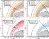 |
Fig. 3 BepiColombo MSB2 and MSB3 trajectories and target magnetosheath intervals in the xy-plane (MASO) at the mean Z locations during the target intervals (ZMASO = −0.3 RM for MSB2 and ZMASO = 0 RM for MSB3). All panels show the BepiColombo swingby trajectory as solid lines in red (MSB2) or blue (MSB3), and the linewidth indicates the Z component (the line gets thinner as the spacecraft moves southbound). The target intervals and center point along the trajectories are denoted with rectangles and white crosses (PICAM time frames are 2022-06-23 09:52–09:53 UTC for MSB2 and 2023-06-19 19:48–19:51 UTC for MSB3). The gray circles, centered on the white crosses, represent the typical propagation distance of a solar wind proton within 1 second: 550 km (panels a, b), 450 km (panel c), and 330 km (panel d). Moreover, the solid black lines in all panels denote the average bow shock and magnetopause boundaries from Winslow et al. (2013) with varying fit parameters, as described in the text. The dash-dotted line shows the magnetopause in another hybrid model study by Fatemi et al. (2018). Panels a and b show shaded areas representing the magnetosheath in the S1, S2, and S3 scenarios. Panels c and d show the magnetosheath in the MSB2 and MSB3 scenarios as red and blue shaded areas, respectively. |
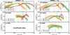 |
Fig. 4 Modeled ion energy distributions for three solar wind scenarios (S1, S2, S3) with a phase space resolution of oMPIC = 3 (left panels) and oMPIC = 15 (right panels). Panels a and d present the distributions obtained using the simple sphere method, while panels b and e used the omnidirectional particle accumulation technique, and panels c and f show the filtered FOV distributions. The solid lines denote the sample mean values within each energy bin, with shaded intervals representing the 95% confidence range. |
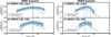 |
Fig. 5 Modeled ion energy distributions comparing the MSB2 (left panels) and MSB3 (right panels) scenarios with a phase space resolution of oMPIC = 50 compared to PICAM measurement data (FOV differential energy flux). Panels a and c display the differential number fluxes calculated using the omnidirectional particle accumulation technique, while panels b and d show the fluxes obtained via the FOV technique. The solid vertical lines represent the sample mean values for each energy bin, with shaded intervals marking the 95% confidence range. |
4 Summary and discussion
We have presented a new method for comparing numerical model results with measurement data that incorporates the FOV, thus distinguishing it from similar but omnidirectional approaches used in previous studies (Jarvinen et al. 2018; Lavorenti et al. 2022; Aizawa et al. 2022). We applied three different concepts with increasing complexity to simulated particle data from the global 3D hybrid simulation model AIKEF to obtain ion energy distributions within the magnetosheath of Mercury. More specifically, we calculated omnidirectional and FOV differential energy fluxes. We presented three scenarios by varying the solar wind input parameters (minimum, average, maximum). These scenarios allowed us to assess the overall systematic deviations and demonstrate, for example, that the solar wind speed directly affects the energy of magnetosheath particles. As expected from the Rankine-Hugoniot jump conditions, a higher upstream solar wind velocity results in higher average ion speeds in the magnetosheath. In addition to changing the physical input parameters, we used different phase space resolutions (oMPIC) to show the effect on particle fluxes. Additionally, we ran dedicated simulations for BepiColombo MSB2 and MSB3. In these simulations, we initialized the model with solar wind and IMF parameters based on our current best estimates obtained from solar wind upstream measurement data, which were measured right after the flybys with the PICAM and MGF instruments. In each run, we assessed the stochastic deviations in the model results by using statistical confidence intervals. We took 100 realizations (or 22 seconds) as a basis to evaluate these confidence intervals. This helped cover smaller dynamics within the given quasi-stationary simulation result. The systematic deviations introduced by varying the input parameters are approximately two (FOV) to five (omni) times larger than the stochastic variations observed within individual model runs, highlighting the dominance of systematic effects in influencing the energy distributions. The general comparison of our modeled bow shock and magnetopause positions with the boundary conditions obtained by Winslow et al. (2013) shows that for similar input parameters (Pram and MA), we get smaller stand-off distances, although these still fall within the uncertainties of their study. A better fit for the magnetopause position is achieved by comparing to hybrid modeling results by Fatemi et al. (2018).
Generally, the sphere method can give a rough overview of the plasma environment; however, it averages over different particle populations, solar wind, and magnetosheath particles, thus “blurring” the bow shock boundary. Additionally, due to the large spherical volume, low energy particles are overestimated in the flux calculation, as time of flight is neglected and low energy particles far from the trajectory are counted. This effect is mitigated in the omnidirectional and FOV methods. It is important to note that we assumed a constant particle velocity over the accumulation time Δt. If particles experience significant acceleration or deceleration (due to electromagnetic fields, collisions, etc.), this assumption does not hold, and particles may not end up in the expected distance bin. A longer Δt results in larger bins, which in the current method is not useful due to the assumption of constant particle velocities. Conversely, a shorter Δt leads to smaller bins and consequently lower count rates. We selected Δt = 1 sec ≈ 4 ·ΔtPICAM as a practical compromise. This choice ensures a sufficient number of counts per bin and simplifies flux normalization.
Nevertheless, we successfully show that measured differential energy flux distributions by the PICAM instrument lie within the lower end of the confidence intervals (the stochastic deviation) of the simulated data using the same FOV as PICAM during the flybys. Overall, the magnitude of the mean fluxes are up to ten times higher than the measured values. This discrepancy primarily arises from the assumptions used in the flux calculation and could be corrected by applying an offset factor, which is not implemented in this study. The need for such a factor to improve agreement with measurements will be assessed in future studies, which will also consider different plasma regions.
In both MSB2 and MSB3, the peak energy of the flux distributions align well with the measurement with a deviation of less than 50 eV. The modeled high-energy tails in both scenarios exhibit a flatter decline, resulting in higher fluxes at higher energies compared to the measurements. Possible reasons for deviations, apart from inherent measurement errors, include systematic offsets due to a changing solar wind input or the fact that only one species (protons) was considered in the solar wind inflow. Heavier species could contribute to the flux observed in the magnetosheath and potentially increase the flux. On the other hand, numerical factors in the FOV technique may underestimate flux in lower energy bins. This is because the bin volume decreases as energy decreases, leading to a reduced particle count. A higher phase space resolution mitigates this issue, and therefore the MSB2 and MSB3 scenarios use a higher phase space resolution (oMPIC = 50) in order to be specifically compared to measurement data. The peak energies of the modeled MSB2 flux for the omnidirectional and FOV methods are the same. While this indicates no directional (FOV) dependency of the flux, it is important to note that the flux lines plotted are binned and maxima positions are therefore quantized.
Changing the model’s input parameters, both physical and numerical, can alter the classification of a fixed spatial location. For instance, a point that lies within the magnetosheath under dense but slow solar wind conditions (S1) may instead lie in the solar wind when the solar wind is less dense and faster (S3) since the magnetosphere becomes more compressed. This is the case for the maximum solar wind scenario S3. Along with general simplifications and model assumptions, variations in the input parameters contribute to the largest systematic deviations when compared to measurement data. Even within a realistic range of IMF directions and solar wind properties (S1, S2, S3), the deviations remain significant.
For the omnidirectional and FOV techniques, we chose an inner counting radius of rsat = 200 km for the oMPIC = 3 case and 100 km for the oMPIC = 15 case. These values were determined based on test runs to ensure particle counts exceeded 50 macro-particles. Changing this parameter effects the magnitude of the flux for the omni and FOV methods, as it is used in the normalization parameter A, and more importantly, the change effects the margin of the incidence angle of the particles. If this parameter is set to zero, the particles’ velocity vector would need to be pointing to the exact location along the trajectory, which is usually not the case. If the parameter is set too large, too many (irrelevant) particles are counted that do not even pass near the trajectory point. Additionally, considering the geometry when employing a counting radius such as this, the margin that is created is distance and energy dependent. While ion spectrometers usually use a geometric factor to convert instrumental ion counts to physical values, our aim is to compute fluxes that are directly comparable to ion measurements based on physical parameters within the simulation. In general, the higher the number of particles, the more accurate the representation of the distribution becomes. In the lower resolution case, setting this parameter to ≲200 km results in a very small number of counted particles (in some cases, there are even no counts at all). For instance, this occurs with the FOV approach in the oMPIC = 3 case. The phase space resolution is too low to obtain reasonable particle counts (at least more than three particles per energy bin), and therefore this resolution is insufficient to resolve an FOV spectrum.
In this study, we have considered different phase space resolutions, with oMPIC values ranging from 3 to 50. For the highest-resolution runs (oMPIC = 50), computational resources permitted the resolution of detailed distributions, such as those in panels e and f of Fig. 4. However, we demonstrated that oMPIC = 15 is sufficient to resolve FOV distributions in the magnetosheath and that it offers a balance between computational efficiency and accuracy in our setup. The required oMPIC value may vary depending on the region of interest, on the merging and splitting procedures, and lastly on the specific numerical model employed. It is important to note that if the MPIC value – the actual number of macro-particles per cell – is constant throughout the simulation box, the fidelity is higher in lower density regions due to smaller particle weights. Therefore, the particle splitting and merging procedures used to achieve oMPIC need to be adapted based on the plasma density gradients in the region of interest. For instance, oMPIC can be set proportional to the local plasma density. However, in the magnetosheath interval studied here, where the plasma density is relatively uniform, this effect does not play a significant role.
Finally, while the spatial resolution of the mesh grid (cell distances of 24 km) remains fixed in this work, refining this parameter could allow smaller rsat values to be used, thus enhancing resolution. However, such refinement would come at the cost of longer computational times. Therefore, those who implement this methodology should carefully consider the trade-off between computational time and particle-counting fidelity when selecting Δt, rsat, and oMPIC values.
5 Conclusions
We conclude that, in general, it is possible to use an FOV technique to obtain proton differential energy flux if the phase space resolution is large enough (oMPIC > 15 in our specific model). The significant fluctuations in the solar wind and IMF at Mercury’s orbit, combined with Mercury’s weak intrinsic magnetic field, result in a highly dynamic interaction (Winslow et al. 2013). We identify this variability as potentially the largest systematic deviation. Direct and quantitative comparisons between measurements and simulations are possible for dedicated model runs with the expected solar wind conditions. More general model runs, such as using average solar wind scenarios, can still be used as a qualitative reference to in situ measurements.
This work serves as a basis to better compare modeled and measured data and to improve understanding of how measurements may be limited by an instrument’s FOV. By considering the pointing direction of the instrument’s FOV, this study enables the investigation of areas not covered by current mission planning in terms of instrument and spacecraft pointing and can potentially contribute to future or extended mission planning efforts. Future studies should investigate further the accuracy of hybrid simulations in different regions in Mercury’s magnetosphere and validate the results against measurements of the BepiColombo (Benkhoff et al. 2021) and future missions in order to improve the involved models. Additionally, exospheric models could be included into the hybrid plasma models and should be validated by comparison of modeled (FOV) fluxes of different ion species against measurements.
Acknowledgements
This work was financially supported by the Austrian Research Promotion Agency (FFG) ASAP PICAM-4 under contract 885349. WE has been supported by an ESA Research Fellowship. DT is grateful to Uwe Motschmann at the Institut für Theoretische Physik, Technische Universität Braunschweig, Germany, for providing the AIKEF model. The uncalibrated PICAM data is publicly available through ESA’s Planetary Science Archive (PSA, https://psa.esa.int/psa/). The calibrated PICAM data is provided by the instrument team upon request. The preliminary calibrated MGF data can be obtained through personal communication with the Principal Investigator (PI) team or the Science Data Center (SDC) Nagoya (https://miosc.isee.nagoya-u.ac.jp/data/mio.php).
References
- Aizawa, S., Delcourt, D., & Terada, N. 2018, Geophys. Res. Lett., 45, 595 [Google Scholar]
- Aizawa, S., Griton, L. S., Fatemi, S., et al. 2021, Planet. Space Sci., 198, 105176 [Google Scholar]
- Aizawa, S., Persson, M., Menez, T., et al. 2022, Planet. Space Sci., 218, 105499 [Google Scholar]
- Anderson, B. J., Johnson, C. L., Korth, H., et al. 2012, J. Geophys. Res.: Planets, 117, doi:10.1029/2012JE004159 [Google Scholar]
- Bagdonat, T., & Motschmann, U. 2002, J. Computat. Phys., 183, 470 [Google Scholar]
- Baumjohann, W., Matsuoka, A., Narita, Y., et al. 2020, Space Sci. Rev., 216, 125 [Google Scholar]
- Benkhoff, J., van Casteren, J., Hayakawa, H., et al. 2010, Planet. Space Sci., 58, 2 [Google Scholar]
- Benkhoff, J., Murakami, G., Baumjohann, W., et al. 2021, Space Sci. Rev., 217, 90 [Google Scholar]
- Bourgoin, M., & Xu, H. 2014, New J. Phys., 16, 085010 [Google Scholar]
- Dakeyo, J.-B., Maksimovic, M., Démoulin, P., Halekas, J., & Stevens, M. L. 2022, ApJ, 940, 130 [NASA ADS] [CrossRef] [Google Scholar]
- Driscoll, T., & Braun, R. 2022, Fundamentals of Numerical Computation: Julia Edition, Other Titles in Applied Mathematics (Society for Industrial and Applied Mathematics) [Google Scholar]
- ESA SPICE Service 2024, BepiColombo Operational SPICE Kernel Dataset, 10.5270/esa-dwuc9bs [Google Scholar]
- Exner, W., Simon, S., Heyner, D., & Motschmann, U. 2020, J. Geophys. Res. (Space Phys.), 125, e27691 [Google Scholar]
- Exner, W., Griton, L., & Heyner, D. 2024, J. Geophys. Res. (Space Phys.), 129, e2023JA032248 [Google Scholar]
- Fang, X., Ma, Y., Masunaga, K., et al. 2017, J. Geophys. Res.: Space Phys., 122, 4117 [Google Scholar]
- Fatemi, S., Poppe, A., Delory, G., & Farrell, W. 2017, J. Phys.: Conf. Ser., 837, 012017 [Google Scholar]
- Fatemi, S., Poirier, N., Holmström, M., et al. 2018, A&A, 614, A132 [NASA ADS] [CrossRef] [EDP Sciences] [Google Scholar]
- Fatemi, S., Hamrin, M., Krämer, E., et al. 2024, MNRAS, 531, 4692 [Google Scholar]
- Griton, L., Issautier, K., Moncuquet, M., et al. 2023, A&A, 670, A174 [NASA ADS] [CrossRef] [EDP Sciences] [Google Scholar]
- Herčík, D., Trávníček, P. M., Johnson, J. R., Kim, E.-H., & Hellinger, P. 2013, J. Geophys. Res.: Space Phys., 118, 405 [Google Scholar]
- James, M. K., Imber, S. M., Bunce, E. J., et al. 2017, J. Geophys. Res.: Space Phys., 122, 7907 [Google Scholar]
- Jarvinen, R., Brain, D. A., Modolo, R., Fedorov, A., & Holmström, M. 2018, J. Geophys. Res.: Space Phys., 123, 1678 [Google Scholar]
- Jarvinen, R., Alho, M., Kallio, E., & Pulkkinen, T. I. 2020, MNRAS, 491, 4147 [NASA ADS] [CrossRef] [Google Scholar]
- Jia, X., Slavin, J. A., Gombosi, T. I., et al. 2015, J. Geophys. Res.: Space Phys., 120, 4763 [Google Scholar]
- Jia, X., Slavin, J. A., Poh, G., et al. 2019, J. Geophys. Res.: Space Phys., 124, 229 [Google Scholar]
- Kiyani, K. H., Osman, K. T., & Chapman, S. C. 2015, Philos. Trans. Roy. Soc. A: Math. Phys. Eng. Sci., 373, 20140155 [Google Scholar]
- Lai, S. H., Yang, Y.-H., & Ip, W.-H. 2024, ApJ, 961, 83 [Google Scholar]
- Lapenta, G., Schriver, D., Walker, R. J., et al. 2022, J. Geophys. Res. (Space Phys.), 127, e30241 [Google Scholar]
- Lavorenti, F., Henri, P., Califano, F., et al. 2022, A&A, 664, A133 [NASA ADS] [CrossRef] [EDP Sciences] [Google Scholar]
- Lu, Q., Guo, J., Lu, S., et al. 2022, ApJ, 937, 1 [NASA ADS] [CrossRef] [Google Scholar]
- Müller, J., Simon, S., Motschmann, U., et al. 2011, Comput. Phys. Commun., 182, 946 [Google Scholar]
- Müller, J., Simon, S., Wang, Y.-C., et al. 2012, Icarus, 218, 666 [CrossRef] [Google Scholar]
- Orsini, S., Livi, S., Torkar, K., et al. 2010, Planet. Space Sci., 58, 166 [Google Scholar]
- Orsini, S., Livi, S. A., Lichtenegger, H., et al. 2021, Space Sci. Rev., 217, 11 [Google Scholar]
- Palmroth, M., Ganse, U., Pfau-Kempf, Y., et al. 2018, Living Rev. Computat. Astrophys., 4, 1 [Google Scholar]
- Paral, J., & Rankin, R. 2013, Nat. Commun., 4, 1645 [Google Scholar]
- Paral, J., Trávníček, P. M., Rankin, R., & Schriver, D. 2010, Geophys. Res. Lett., 37, doi:10.1029/2010GL044413 [Google Scholar]
- Rao, S. S. 2010, The Finite Element Method in Engineering (Elsevier) [Google Scholar]
- Schulz, H. E., Simoes, A. L. A., & Lobosco, R. J. 2011, Hydrodynamics (Rijeka: IntechOpen) [Google Scholar]
- Shadwick, B. A., Stamm, A. B., & Evstatiev, E. G. 2014, Phys. Plasmas, 21, 055708 [Google Scholar]
- Slavin, J. A., Acuña, M. H., Anderson, B. J., et al. 2009, Science, 324, 606 [NASA ADS] [CrossRef] [Google Scholar]
- Slavin, J. A., DiBraccio, G. A., Gershman, D. J., et al. 2014, J. Geophys. Res. (Space Phys.), 119, 8087 [Google Scholar]
- Slavin, J. A., Imber, S. M., & Raines, J. M. 2021, Magnetosph. Solar Syst., 535 [Google Scholar]
- Smith, D. E., Zuber, M. T., Phillips, R. J., et al. 2012, Science, 336, 214 [NASA ADS] [CrossRef] [Google Scholar]
- Solomon, S. C., McNutt, R. L., Gold, R. E., & Domingue, D. L. 2007, Space Sci. Rev., 131, 3 [Google Scholar]
- Sun, W., Dewey, R. M., Aizawa, S., et al. 2022, Sci. China Earth Sci., 65, 25 [Google Scholar]
- Teubenbacher, D., Exner, W., Feyerabend, M., et al. 2024, A&A, 681, A98 [NASA ADS] [CrossRef] [EDP Sciences] [Google Scholar]
- Trávníček, P., Hellinger, P., & Schriver, D. 2007, Geophys. Res. Lett., 34, doi:10.1029/2006GL028518 [Google Scholar]
- Trávníček, P. M., Hellinger, P., Schriver, D., et al. 2009, Geophys. Res. Lett., 36, doi:10.1029/2008GL036630 [Google Scholar]
- Trávníček, P. M., Schriver, D., Hellinger, P., et al. 2010, Icarus, 209, 11 [CrossRef] [Google Scholar]
- Varela, J., & Pantellini, F. 2023, A&A, 675, A148 [NASA ADS] [CrossRef] [EDP Sciences] [Google Scholar]
- Vernisse, Y., Riousset, J., Motschmann, U., & Glassmeier, K.-H. 2018, Planet. Space Sci., 152, 18 [Google Scholar]
- Winske, D., & Omidi, N. 1996, J. Geophys. Res.: Space Phys., 101, 17287 [Google Scholar]
- Winslow, R. M., Anderson, B. J., Johnson, C. L., et al. 2013, J. Geophys. Res. (Space Phys.), 118, 2213 [NASA ADS] [CrossRef] [Google Scholar]
All Tables
All Figures
|
Fig. 1 Trajectories and target magnetosheath interval. Panel a shows the top view (xy-plane), panel b shows the side view from the dawnside (xz-plane), and panel c shows the view from the back (yz-plane). MASO coordinates are used. The BepiColombo MSB2 and MSB3 trajectories are respectively shown with a solid red and solid blue line, and the PICAM measurement time frames are indicated in rectangles. Models for the magnetopause and bow shock are illustrated by the black dashed (Winslow et al. 2013) and black solid (Slavin et al. 2009; Winslow et al. 2013) lines at X, Y, Z = 0, respectively. |
| In the text | |
|
Fig. 2 Field-of-view particle counting schemata. Panel a shows the sphere method, panel b shows the omnidirectional method, and panel c shows the FOV method. The purple line shows an arbitrary spacecraft trajectory, rsat is the base circle to count incident particles, γ is the cone opening angle, and dmax is the maximum counting distance from the base circle. The dots show example particles with their velocity vectors. While the green particles were counted, the red ones were neglected, as (1) they are located outside the cone or their distance to the base circle is larger than dmax, (2) they are inside the cone but do not intersect the base circle, or (3) they are inside the cone pointing toward the base circle, but their energy and distance do not correspond to the criterion mentioned in the text. The coordinates are given in MASO (explained in the text) shifted to the center of each trajectory point. |
| In the text | |
|
Fig. 3 BepiColombo MSB2 and MSB3 trajectories and target magnetosheath intervals in the xy-plane (MASO) at the mean Z locations during the target intervals (ZMASO = −0.3 RM for MSB2 and ZMASO = 0 RM for MSB3). All panels show the BepiColombo swingby trajectory as solid lines in red (MSB2) or blue (MSB3), and the linewidth indicates the Z component (the line gets thinner as the spacecraft moves southbound). The target intervals and center point along the trajectories are denoted with rectangles and white crosses (PICAM time frames are 2022-06-23 09:52–09:53 UTC for MSB2 and 2023-06-19 19:48–19:51 UTC for MSB3). The gray circles, centered on the white crosses, represent the typical propagation distance of a solar wind proton within 1 second: 550 km (panels a, b), 450 km (panel c), and 330 km (panel d). Moreover, the solid black lines in all panels denote the average bow shock and magnetopause boundaries from Winslow et al. (2013) with varying fit parameters, as described in the text. The dash-dotted line shows the magnetopause in another hybrid model study by Fatemi et al. (2018). Panels a and b show shaded areas representing the magnetosheath in the S1, S2, and S3 scenarios. Panels c and d show the magnetosheath in the MSB2 and MSB3 scenarios as red and blue shaded areas, respectively. |
| In the text | |
|
Fig. 4 Modeled ion energy distributions for three solar wind scenarios (S1, S2, S3) with a phase space resolution of oMPIC = 3 (left panels) and oMPIC = 15 (right panels). Panels a and d present the distributions obtained using the simple sphere method, while panels b and e used the omnidirectional particle accumulation technique, and panels c and f show the filtered FOV distributions. The solid lines denote the sample mean values within each energy bin, with shaded intervals representing the 95% confidence range. |
| In the text | |
|
Fig. 5 Modeled ion energy distributions comparing the MSB2 (left panels) and MSB3 (right panels) scenarios with a phase space resolution of oMPIC = 50 compared to PICAM measurement data (FOV differential energy flux). Panels a and c display the differential number fluxes calculated using the omnidirectional particle accumulation technique, while panels b and d show the fluxes obtained via the FOV technique. The solid vertical lines represent the sample mean values for each energy bin, with shaded intervals marking the 95% confidence range. |
| In the text | |
Current usage metrics show cumulative count of Article Views (full-text article views including HTML views, PDF and ePub downloads, according to the available data) and Abstracts Views on Vision4Press platform.
Data correspond to usage on the plateform after 2015. The current usage metrics is available 48-96 hours after online publication and is updated daily on week days.
Initial download of the metrics may take a while.