| Issue |
A&A
Volume 656, December 2021
|
|
|---|---|---|
| Article Number | A73 | |
| Number of page(s) | 20 | |
| Section | Planets and planetary systems | |
| DOI | https://doi.org/10.1051/0004-6361/202140551 | |
| Published online | 06 December 2021 | |
The New Generation Planetary Population Synthesis (NGPPS)
V. Predetermination of planet types in global core accretion models
1
Max-Planck-Institut für Astronomie,
Königstuhl 17,
69117
Heidelberg,
Germany
e-mail: This email address is being protected from spambots. You need JavaScript enabled to view it.
2
David A. Dunlap Department of Astronomy & Astrophysics, University of Toronto,
50 St. George St.,
Toronto,
ON
M5S 3H4,
Canada
3
Carl Sagan Institute, Cornell University,
Ithaca,
NY
14853,
USA
4
Physikalisches Institut, University of Bern,
Gesellschaftsstrasse 6,
3012
Bern,
Switzerland
5
Lunar and Planetary Laboratory, University of Arizona,
1629 E. University Blvd.,
Tucson,
AZ
85721,
USA
6
Geneva Observatory, University of Geneva,
Chemin Pegasi 51b,
1290
Versoix,
Switzerland
Received:
12
February
2021
Accepted:
20
April
2021
Abstract
Context. State-of-the-art planet formation models are now capable of accounting for the full spectrum of known planet types. This comes at the cost of an increasing complexity of the models, which calls into question whether established links between their initial conditions and the calculated planetary observables are preserved.
Aims. In this paper, we take a data-driven approach to investigate the relations between clusters of synthetic planets with similar properties and their formation history.
Methods. We trained a Gaussian mixture model on typical exoplanet observables computed by a global model of planet formation to identify clusters of similar planets. We then traced back the formation histories of the planets associated with them and pinpointed their differences. Using the cluster affiliation as labels, we trained a random forest classifier to predict planet species from properties of the originating protoplanetary disk.
Results. Without presupposing any planet types, we identified four distinct classes in our synthetic population. They roughly correspond to the observed populations of (sub-)Neptunes, giant planets, and (super-)Earths, plus an additional unobserved class we denote as “icy cores”. These groups emerge already within the first 0.1 Myr of the formation phase and are predicted from disk properties with an overall accuracy of >90%. The most reliable predictors are the initial orbital distance of planetary nuclei and the total planetesimal mass available. Giant planets form only in a particular region of this parameter space that is in agreement with purely analytical predictions. Including N-body interactions between the planets decreases the predictability, especially for sub-Neptunes that frequently undergo giant collisions and turn into super-Earths.
Conclusions. The processes covered by current core accretion models of planet formation are largely predictable and reproduce the known demographic features in the exoplanet population. The impact of gravitational interactions highlights the need for N-body integrators for realistic predictions of systems of low-mass planets.
Key words: planets and satellites: formation / protoplanetary disks / planets and satellites: dynamical evolution and stability / planet-disk interactions / methods: numerical / methods: statistical
© M. Schlecker et al. 2021
 Open Access article, published by EDP Sciences, under the terms of the Creative Commons Attribution License (https://creativecommons.org/licenses/by/4.0), which permits unrestricted use, distribution, and reproduction in any medium, provided the original work is properly cited.
Open Access funding provided by Max Planck Society.
1 Introduction
One of the most remarkable findings in recent years of exoplanetology has been the enormous diversity of planetary systems (e.g., Ribas & Miralda-Escudé 2007; Howard et al. 2012; Fressin et al. 2013; Petigura et al. 2013; Mulders et al. 2015; Hobson & Gomez 2017; Brewer et al. 2018; Owen & Murray-Clay 2018; Hsu et al. 2019; Bryan et al. 2019; He et al. 2020). The rapidly increasing number of confirmed planets improves our ability to explore this diversity and to understand its origins. To this end, a variety of physical mechanisms that influence the formation and evolution of planetary systems, and therefore shape their demographics, have been investigated. Intensively studied mechanisms include the evolution of accretion disks (e.g., Lüst 1952; Lynden-Bell & Pringle 1974; Pringle 1981), their interaction with embedded planets that may result in orbital migration (e.g., Goldreich & Tremaine 1979; Tanaka et al. 2002; D’Angelo et al. 2003; Paardekooper et al. 2011; Dittkrist et al. 2014), how these protoplanets form and grow by accreting solid components and gas (e.g., Bodenheimer & Pollack 1986; Ida & Makino 1993; Pollack et al. 1996; Thommes et al. 2003; Fortier et al. 2013), their gravitational interaction among each other (e.g., Chambers et al. 1996; Raymond et al. 2009), photoevaporation of both protoplanetary disks (Hollenbach et al. 1994; Clarke et al. 2001; Alexander et al. 2014) and planetary atmospheres (Lammer et al. 2003; Owen & Jackson 2012; Jin et al. 2014), and the long-term evolution of planets and their atmospheres (e.g., Bodenheimer & Pollack 1986; Guillot 2005; Fortney & Nettelmann 2010; Mordasini et al. 2012c). While all of these processes leave an imprint on the final planetary systems, observing them while they are in action has proven to be very challenging and was possible only in rare cases (e.g., Keppler et al. 2018). Global models of planet formation can mitigate this shortcoming by combining as many relevant physical processes as possible and simulating the growth and evolution of planets in an end-to-end fashion. Thereby, they provide a link between properties of disks and observables of the resulting planets. When employed within a Monte Carlo experiment with distributions of initial conditions, synthetic planet populations can be produced and statistically evaluated (e.g., Ida & Lin 2004a; Mordasini et al. 2009; Ndugu et al. 2018). Such population synthesis frameworks are increasingly able to produce different kinds of planets, from terrestrial-sized rocky planets to gas giants, using the same formation model.
The core accretion scenario (Perri & Cameron 1974; Mizuno et al. 1978; Mizuno 1980), in which a solid planetary core forms that may subsequently accrete a gaseous envelope, has been recognized as the most common planetary formation avenue. Concerning the problem of how this solid core grows, two different approaches have emerged: Commonly, the growth of the solid component has been modeled as the accretion of ~kilometer-sized planetesimals (e.g., Ida & Makino 1993; Thommes et al. 2003). Under this assumption, the thresholds in the disk properties responsible for the emergence of different planet types are determined by the availability of planetesimals at the position of a growing planet and by the timescale for accreting them (Lissauer 1987, 1993; Kokubo & Ida 2000). In recent years, a growing body of literature includes the accretion of millimeter- to centimeter-sized “pebbles”, whose motions are decoupled from the gas disk (Ormel & Klahr 2010; Lambrechts & Johansen 2012; Bitsch & Johansen 2017). Here, the resulting radial motion of the particles causes an interrelation between the inner and outer regions of the disk (Morbidelli & Nesvorny 2012; Lambrechts & Johansen 2014; Ormel et al. 2017).
Both approaches have allowed the unambiguous predetermination of planetary parameters from initial conditions (e.g., Kokubo & Ida 2002; Ida & Lin 2004b; Lin et al. 2018). However, with ever more sophisticated models of increasing complexity, it is uncertain whether these relationships persist. In particular, the inclusion of an N-body treatment ofprotoplanets could destroy these connections due to the chaotic component it introduces. A number of studies have addressed this problem in different ways, either by categorizing the outcomes of simulations with different initial conditions (Mordasini et al. 2009, 2012a; Bitsch et al. 2015, 2018; Miguel et al. 2020), or by relating synthetic populations to the observed sample of exoplanets (Mordasini et al. 2009; Chambers 2018; Fernandes et al. 2019; Mulders et al. 2020) or transitional disks (Chaparro Molano et al. 2019). A main limitation of these advances has been their restriction to a particular region of the planetary parameter space.
Recent advancements of our formation model (Emsenhuber et al. 2021a) now allow for an extension of these investigations to the full range of currently known planet types. Therefore, in this study, we statistically assess the relations between a number of relevant disk properties and the emerging planet types in the context of the core accretion paradigm. To this end, we investigate synthetic planet populations computed with the Generation III Bern Model of planet formation and evolution (Emsenhuber et al. 2021a, hereafter Paper I). Previous papers in this series have presented populations from this model with different numbers of planets per system (Emsenhuber et al. 2021b, Paper II) and varying host star masses (Burn et al. 2021, Paper IV). Here, we focus on two populations of systems around solar-type stars: NG73 for isolated single planets, and NG76 with 100 planetary embryos growing concurrently (Paper II). We thereby take care to follow a purely data-driven approach and do not presuppose planet types motivated by observations or theoretical arguments.
This paper is divided into six sections. In Sect. 2, we describe the formation model and introduce the synthetic planet populations. We then present a cluster analysis performed on these populations in Sect. 3. Section 4 investigates to what degree the identified clusters of similar planets can be predicted from properties of protoplanetary disks. In Sect. 5, we interpret our results and discuss their implications for planet formation. We conclude by summarizing our findings in Sect. 6.
2 Planet population synthesis
This work analyzes synthetic planet populations for solar-mass host stars from the Generation III Bern global model of planet formation and evolution (Paper I). The formation part of the model combines the evolution of a protoplanetary disk with both gas and solid components, the growth and determination of the internal structure of protoplanets, their dynamical interactions, and gas-driven planetary migration.
The gas disk is modeled as a viscously accreting disk (Lüst 1952; Lynden-Bell & Pringle 1974; Pringle 1981) with an α-parametrization (Shakura & Sunyaev 1973) for the turbulent viscosity. The vertical structure is computed following Nakamoto & Nakagawa (1994) and Hueso & Guillot (2005) under an evolving luminosity of the star (Baraffe et al. 2015). The solid disk component is modeled in a fluid-like description where the dynamical state of planetesimals is given by the stirring due to other planetesimals and protoplanets (Thommes et al. 2003; Chambers 2006; Fortier et al. 2013).
The formation of protoplanets follows the core accretion paradigm (Perri & Cameron 1974; Mizuno et al. 1978; Mizuno 1980) with planetesimal accretion in the oligarchic regime (Ida & Makino 1993). We calculated the structure of the planetary envelopes by directly solving one-dimensional internal structure equations (Bodenheimer & Pollack 1986). Initially, gas accretion is limited by the ability of the planet to radiate away the gravitational energy release by accretion of solids and gas (Pollack et al. 1996; Lee & Chiang 2015). At this stage, the internal structure is used to compute the gas accretion rate. Once a planet exhausts the supply from the gas disk (either because cooling becomes efficient or because the disk disperses), the envelope is no longer in equilibrium with the disk and contracts (Bodenheimer et al. 2000). In this detached phase, the internal structure equations are used to determine the planet’s radius. The formation stage also includes gas-driven planetary migration in the Type I (Paardekooper et al. 2011) and Type II (Dittkrist et al. 2014) regimes.
The planetary seeds start with a mass of 0.01 M⊕ and are inserted with random initial orbital distances astart drawn from a log-uniform distribution between the inner disk edge and 40 au. When multiple embryos are present in the same disk, their gravitational interactions are modeled during the first 20 Myr using the Mercury N-body integrator (Chambers 1999). After this time, the model switches to the evolutionary stage. Here, the thermodynamical evolution is calculatedfor each planet individually up to a simulation time of 10 Gyr. This stage includes atmospheric loss via photoevaporation (Jin et al. 2014) and tidal migration. As a result, the model is able to compute the planets’ masses, radii, and luminosities as a function of time. For a thorough description of the Generation III Bern Model and an outline of recent advancements of the framework (Alibert et al. 2005, 2013; Mordasini et al. 2009, 2012c,b), we refer to Paper I.
Synthetic planet populations are produced by running the model in a Monte Carlo scheme, where initial conditions are drawn randomly from distributions motivated by observational (Santos et al. 2003; Lodders 2003; Andrews et al. 2010; Venuti et al. 2017; Ansdell et al. 2018; Tychoniec et al. 2018) or theoretical constraints (Dra̧zkowska et al. 2016; Lenz et al. 2019). The distributed variables include the initial gas disk mass Mgas, the inner edge of the disk rin, its dust-to-gas ratio ζd,g, the mass loss rate due to photoevaporative winds Ṁwind, and the starting locations of the planetary seeds astart. The values or distributions of all model parameters are listed in Table 1 and are motivated in detail in Paper I and Paper II.
Our goal is to uncover characteristic links between these properties and the emerging planet types, which requires to robustly define the latter first. This step may be impaired by the stochasticity of an N-body treatment that smears the boundaries between clusters of similar planets. We thus examine both a population with a single planet per system and a population with multiple planets per system. For the single-planet population, called NG73, 30 000 systems were simulated. In 29 455 systems, the planet was not accreted onto the star and is still present after 5 Gyr, which we consider as time of observation.
To consider the impact of gravitational interactions among planets, we investigate the multi-planet population NG76 and compare it to the single-planet case. In each of its systems, an initial set of 100 protoplanets competed for material and interacted gravitationally. All other boundary conditions were left the same, and the Monte Carlo parameters were drawn from the same distributions. The N-body module integrated for 20 Myr to cover the entire formation phase with planets still embedded in the disk, as well as an appropriate subsequent evolutionary era without disk interactions (Paper I). Out of the 1000 simulated systems, 32 030 planets survived until t = 5 Gyr. For detailed descriptions of both planet populations, see Paper II and Schlecker et al. (2021), Paper III.
Choice of model parameters.
3 Cluster analysis
A cluster analysis aims at identifying groups of entities that share similar properties in a specific set of parameters. In our case, we aim to explore which distinct planet species emerge from our planet formation model and how they compare to observed (exo-)planet types. Accordingly,we chose as training features three parameters typically obtained from exoplanet observations: the orbital semi-major axis a, the planet mass MP, and the planet radius RP. Our clustering was done in a purely data-driven fashion and without any prior knowledge on existing or expected planet types. The only information our clustering model received was a snapshot of our synthetic planet population at a simulation time of 5 Gyr.
3.1 Data preparation
In general, clustering methods are not scale-invariant (Jain & Dubes 1988). The application of cluster algorithms to unevenly scaled data sets can thus lead to compromised results. Based on the distribution of the parameters of interest in our data set, we rescaled the features a, MP, and RP by applying a log10.
3.2 Model selection and hyperparameters
We performed the clustering using Gaussian mixture models (GMMs, McLachlan 1988), a class of hierarchical, probabilistic clustering algorithms. A GMM consists of multiple components i = 1⋯ N of multivariate normal distributions, each characterized by its weight ϕi, its mean μi, and its covariance matrix Σi. The model then takes the form
 (1)
(1)
During training on a data set, the parameters ϕi, μi, and Σi are updated using the expectation-maximization (EM) algorithm (Hartley 1958). A free hyperparameter is the number of Gaussian components N, that is, the number of Gaussian distributions the data points are assumed to be generated from. The trained GMM gives each data point a set of N probabilities, corresponding to the probability that the data point belongs to a specific component i. When we classified our data, we assigned each planet the component (that is, the planet cluster) with the highest probability.
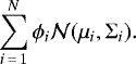
Since GMM, and clustering algorithms in general, are unsupervised methods, the selection of a “best” model has to be seen in the context of the goal we want to achieve. We aimed at identifying groups of planets based on overdensities in the planetary parameter space, regardless of their shape. With this goal in mind, we have explored several other algorithms in addition to GMM and found that they consistently performed worse on our data set (see Appendix A). Using the scikit-learn (Pedregosa et al. 2011) implementation of GMM with default arguments, the only free hyperparameter was the number of clusters in the data N. In finding the optimal choice of N, we were aided by several validation metrics. We considered the Akaike Information Criterion (AIC, Akaike 1973; Cavanaugh & Neath 2019), the Bayesian Information Criterion (BIC, Schwarz 1978), the Davies-Bouldin score (DB, Davies & Bouldin 1979), the CaliÅski-Harabasz score (CH, Caliñski & Harabasz 1974), and the Silhouette score (Rousseeuw 1987). These metrics assess clustering performance with different approaches, and due to the complex structures in our data they can contradict each other. We provide a detailed description of the different metrics in Appendix A.2. For now, it is important to note that AIC, BIC, and DB should be minimized, and CH and the Silhouette score should be maximized. In Fig. 1, we show the different scores for GMMs with N ∈ [3...10] upon applying them to our single-planet (NG73) and multi-planet (NG76) population, respectively. For NG73, two potential choices stick out, N = 4 and N = 6. To decide between these options, we produced diagnostic scatter plots where all possible 2D projections of the planetary parameter space are shown with planets color-coded by cluster affiliation. The plots for the candidate models are shown in Fig. A.2. While human bias might be an issue at this step, we took care to judge the clustering only based on over- and underdensities of planets and not based on where we expected different planet types. We found that the GMM with N = 4 performed best. For NG76, both N = 3 and N = 5 yielded promising scores. By judging the corresponding diagnostic plots, we concluded that N = 5 clusters is the preferred mode. With all hyperparameters fixed, we performed the unsupervised training of our nominal GMMs on the full data sets and considering full covariance matrices.
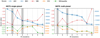 |
Fig. 1 Validation scores for GMMs with different numbers of components N. For AIC, BIC, and DB (top panels), lower values are preferred; and for Silhouette score and CH (bottom panels), higher values are preferred. AIC and BIC generally show indistinguishable values. Based on these scores, sensible choices are N = 4 and N = 6 for NG73, and N = 3 and N = 5 for NG76 (highlighted in gray). We note the different y-axis scales. |
3.3 Detected planet clusters
In the single-planet case, the clustering algorithm identified four separate planet species in our population. Figure 2 shows these clusters in the various projections in {a, MP, RP} space. In general, we notice clear separations between the clusters in all projections, albeit with visible contaminations. Ordered by ascending planetary mass, the clusters are as follows: Clusters 2 and 4 are populations of bare planet cores without atmospheres, and they are cleanly separated in semi-major axis. Both clusters are separatefrom cluster 1, which are close-in planets enhanced in gas and with masses of mostly tens of M⊕. A forth distinct group of very massive planets (MP ≳ 100 M⊕) is formed bycluster 3 with a clear separation from the other species.
Since the GMM is not aware of the underlying physics these clusters result from, it is of interest to interpret the identified clusters and relate them to known planet types. Cluster 2 corresponds to an unobserved population of distant, low-mass planets. As they formed beyond the water ice line and are rich in volatile species, we refer to this group as “icy cores”. Cluster 4 planets are atmosphere-less and rocky, and thus comparable to the observed population of close-in terrestrial planets and super-Earths (e.g., Hsu et al. 2019). By simultaneously taking into account all dimensions of the parameter space, the GMM spatially separated icy cores and (super-)Earths in the region of the water ice line (without any information about its existence). This lead to the clean separation of rocky and icy planets in the MP − RP diagram (diagonal lines in the plot). Cluster 1 roughly corresponds to the observed population of (sub-)Neptunes. In planet radius space, these planets are mostly located above the radius valley (e.g., Fulton et al. 2017; Mordasini 2020, see discussion in Sect. 4.4). There is some contamination by cluster 1 planets in the region of the largest and closest super-Earths, which we attribute to the inability of a GMM to fit a deviation from the otherwise extremely straight line of cluster 4 planets in MP − RP space. Finally, cluster 3 can be identified as gas giant planets. This becomes especially clear in the MP − RP plane, where they occupy the region where in the physical model electron degeneracy occurs. This effect flattens off the mass-radius relation at the high-mass end (e.g., Chabrier et al. 2009).
Figure 3 illustrates the clustering in the multi-planet case, during which we ignored the system affiliation of the planets and treated them as independent entities. Based on the scoring scheme described above, the clearest clustering can be achieved with five components. The overall partitioning appears similar to before, and the fifth component not present in the single-planet population covers planets on distant orbits that have intermediate densities and masses of roughly 0.05 M⊕ to 3 M⊕. We refer to these planets as “icy Earths”. These planets are distributed in a sharp line in mass-radius space, which makes the GMM consider them detached from the more dispersed “icy cores”. Notably, the bulk of the “Neptunes” moved to more distant orbits compared to the single-planet case. This is in line with the observed existence of Neptune-sized planets at orbital distances of several au Suzuki et al. (2016); Kawahara & Masuda (2019). For a comparison of Bern model planets and gravitational microlensing events, we refer to Suzuki et al. (2018).
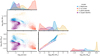 |
Fig. 2 Planet clusters in a 5 Gyr old synthetic planet population with a single planet per system. For all combinations of planet observables a, MP, and RP, the differentcolors denote clusters identified by a four-component Gaussian mixture model (GMM). On the diagonal, we show KernelDensity Estimates of the distributions. Without any information about the physics in our formation model, the GMM identified four planet species roughly corresponding to (sub-)Neptunes (blue), icy cores (red), giant planets (yellow), and (super-)Earths (purple). |
3.4 Model validation
Unlike supervised machine learning algorithms, unsupervised techniques cannot be tested by applying the trained model to a test set due to the lack of “labeled” data. For validation of the clustering itself, we used the aforementioned performance metrics. To evaluate how robust the detected clustering is, we let the model predict the cluster affiliation of a data set of similar structure and compared these predictions to the original clustering. To produce these test data, we employed Gaussian Mixtures of 80 components and full covariance matrices as generative probabilistic models. We trained them on the {a, MP, RP} subspace of the original population synthesis data. The samples drawn from these models show a very similar structure in the whole domain (compare Fig. 4). We note that these “planets” are entirely the product of the generative models and have never been in contact with a physical formation model.
For comparison, we also fed our nominal clustering models with samples drawn from log-uniform distributions with boundaries roughly corresponding to the suprema of the population synthesis data, that is,  and
and 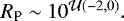 With these pseudo-random data, the models predict clusters that do not resemble the original structures and they appear in most projections almost random. These two tests show that our trained models neither overfit the data set, nor do they produce any clear clusters where none are expected. The generative models can also be used to draw a virtually unlimited number of synthetic planets when the computational costs of employing the full formation model are prohibitive (similar to Mulders et al. 2018).
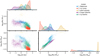 |
Fig. 3 Same as Fig. 2, but for a multi-planet population. The Gaussian mixture model (GMM) prefers solutions including a fifth component of distant, icy planets shown in green. In general, the clusters are less clearly separated than in the single-planet population. |
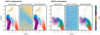 |
Fig. 4 Model validation via generative models. For each of the two planet populations, we show the clustering result of our Gaussian mixture model on population synthesis data (left), random noise (center), and data from a generative model (right). We note that the latter do not stem from a physical formation model but were generated from a high-order GMM that was trained on the original data. The clusters detected in these new data show largely the same structure as the original ones, whereas in the random noise no reliable clusters are found. |
3.5 Planet clustering as a function of simulation time
The cluster analysis took place at a simulation time of t = 5 Gyr. We now trace the identified clusters back in time to investigate their past evolution. Figure 5 shows their position in semi-major axis-mass space at simulation times 0.1 Myr, 0.3 Myr, 0.6 Myr, 1 Myr, 2 Myr, and 10 Myr. In particular in the single-planet population, the clusters occupy distinct domains already at early times and follow characteristic paths in this parameter space. These paths are set by concurrent accretion and planet migration and their respective timescales.
In the following, we focus on the single-planet case where the evolutionary paths can be traced most clearly. At the beginning, all planets are still of such low mass that migration has little effect. Planet growth is determined by the local planetesimal density, feeding zone size, and orbit timescale, and it is most efficient at intermediate orbital distances (Paper II). At a few 105 yr, an outward migration zone located at a few au divides the planetary tracks into two branches. On the outer branch, giant planets evolve similarly as the outer wing of Neptunes. They branch off when runaway gas accretion sets in, while Neptunes continue migrating inward with moderate growth. At later times, another outward migration zone leads to the underdensity in the cluster of close-in (super-)Earths. Icy cores do not exhibit significant growth and largely remain in their initial domain.
Most of the processes that define the different planet types in this parameter space are finished after a few Myr or, at the latest, when the gas disk disperses. Exceptions are atmospheric photoevaporation, which happens on 100 Myr to Gyr timescales (e.g., Lopez et al. 2012; King & Wheatley 2021) and still turns some close-in (sub-)Neptunes into super-Earths, and tidal interaction with the host star affecting some ultra-short period planets. In the case of multiple planets per system, N-body interactions can have an additional long-term impact. A striking result of planet-planet interactions are the significantly lower migration rates compared to the single-planet case, in particular in the Neptunes cluster.
In general, it appears that planet populations form distinct groups very early in the formation process. This begs the question whether the cluster affiliation of a planet can already be predicted from the initial conditions of the simulation.
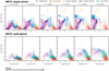 |
Fig. 5 Early time evolution of the clusters identified by the Gaussian mixture model. Each subplot shows a sample of 5000 planets at their current position in semi-major axis-mass space and color-coded by their future cluster affiliation, which is only determined at t = 5 Gyr. Concurrent accretion and migration leads to characteristic evolutionary paths. Distinct groups of planets form already at early simulation times. |
4 Prediction of planet clusters
Our planet formation model provides a deterministic link between properties of protoplanetary disks and properties of planets. This link could be blurred by N-body interactions between the planets, hence in the following experiment we consider first the single-planet population. Our approach was to employ a random forest classifier (Ho 1998; Breiman 2001) to predict the cluster of a planet from its corresponding set of disk properties. Random forests are ensembles of uncorrelated, binary classifiers known as decision trees. Such ensembles achieve strongly improved generalization accuracies compared to single-tree classifiers by constructing trees in pseudorandomly selected feature subspaces (Ho 1995). The individual trees are further decorrelated by drawing, with replacement, random subsets of the input data during training (“bagging”, Breiman 1996).
With varying sizes of the individual clusters (for instance, only ~ 5% of the planets in NG73 are giant planets), our data set is strongly imbalanced. This is problematic for classification algorithms such as random forests, which aim to minimize the overall error rate and thereby tend to neglect minority classes (Chen et al. 2004). To account for this imbalance, we employed a balanced random forest classifier as implemented in the imbalanced-learn1 python package. This variant of random forest randomly under-samples each bootstrap sample on the individual tree level during training (Lemaître et al. 2017).
4.1 Data preparation, hyperparameters, and training
Our classifier learned rules based on four features: the initial gas disk mass Mgas,0, the initial solid disk mass Msolid,0, the initial orbital distance of the planetary embryo astart, and the disklifetime tdisk. The solid disk mass is a derived quantity that we computed from the gas disk mass and host star metallicity. We rescaled these features to account for their large differences in scale: tdisk and astart were transformed by a log10 function, and Mgas,0 and Msolid,0 were modified to roughly Gaussian distributions by the Box-Cox transform (Box & Cox 1964). The clustering above assigned each synthetic planet a probability to belong to each of the clusters. For the subsequent analysis, we avoided planets that cannot be mapped clearly to a cluster and kept only those with a probability of affiliation > 0.99. This decreased our sample from 29 455 to 23 278 planets. Finally, we divided the data into a random subset containing 80% of the initial data for training and a test set with the remaining 20% to determine the performance of the classifier. The resulting training set contains between 1059 (giant planets) and 8486 ((super-)Earths) planets per cluster. We trained an ensemble of 500 fully grown estimators, that is, without reducing the depth of the trees by pruning them, on this set.
4.2 Error and performance analysis
To measure the generalization performance of the trained model already during its development, we predicted clusters from the out-of-bag samples, which were never seen by the respective estimator during training. The average of the resulting out-of-bag score produces an estimate for the accuracy of the entire ensemble, and we obtained a score of 98% here. However, classification accuracy is not a sufficient performance measure since we are dealing with a strongly skewed data set. In the following, we investigate the types of errors our model makes and measure its performance.
We computed a confusion matrix using five-fold cross-validation. For this purpose, the data set was randomly split into five evenly sized folds; the model was trained five times on 5 − 1 = 4 folds, and then evaluated on the fold it was not trained on. The left panel of Fig. 6 shows the confusion matrix produced from the labeled training set and the predictions from cross-validation. Rows correspond to the actual clusters, and columns are the predictions of our model. Each field xi,j in the matrix shows the fraction of times a planet of cluster i was classified as a planet of cluster j. Most planets fall into the diagonal, meaning a correct classification. All clusters are predicted with more than 95% accuracy and the largest errors occur for clusters 2 and 3. The right panel of the figure shows the same matrix with the correct classifications removed and the color map rescaled. It is obvious that the errors are largely symmetric. The highest rate of misclassification occurred between clusters 2 and 3 (3% of icy cores were confused with giant planets and vice-versa). The reason is that the former are frequently progenitors of the latter, and prediction of those planets thatjust (do not) reach the conditions for runaway gas accretion is difficult (compare Fig. 2).
To estimate the generalization error the model makes when applied to data not part of the training set, we measured its performanceon the test set of 4656 systems we held out before. Based on five-fold cross-validation, it achieves an overall accuracy of 97% and misclassifications occur between the same clusters as seen in the training set. This shows that the model is not significantly overfitted.
Feature importances of disk properties.
4.3 Results of planet predictions
4.3.1 Correlations with disk properties
For each of the clusters identified in Sect. 3.3, we show the distributions and pairwise relationships of their corresponding disk properties in Fig. 7. Underdensities in the scatter plots are due to removed planets of ambiguous cluster affiliation. Unsurprisingly, giant planets (yellow) grow in disks with large reservoirs of solid material Msolid and high gas mass Mgas. It is evident that most of these clusters, which are labeled at “observation time” t = 5 Gyr, form groups already in this parameter space, that is, before the simulations started. However, they differentiate distinctly only in the projections involving the start position of planetary embryos astart. The separation is especially clear in astart − Msolid,0 space, which shows the least overlap of different clusters. With increasing initial orbital distance, the dominant planet species are (super-)Earths, Neptunes, giant planets, and icy cores.
4.3.2 Feature importance
Our classification model reaches high accuracies for all planet clusters, but it is interesting to see which disk features are most important for a successful classification. This is possible by measuring the feature importance of the data set given to the model using the Mean Decrease Impurity (MDI, Breiman et al. 1984). MDI quantifies to what extent a feature reduces the impurity of the trees in the random forest. Put simply, it is a measure of how well the nodes can use the feature to split the data set into “pure” child nodes, each containing only data of a single label. A higher score means that the feature is more important for correct classification. We list the MDI for each input parameter in Table 2. With a score of 0.68, the starting position of the planetary core astart is clearly the parameter most sensitive for predicting a planet’s cluster. The gaseous mass of the disk and its lifetime are the least important features.
However, the degree of dependency on certain disk features varies from cluster to cluster. To get a cluster-specific insight, we multiply for each cluster the mean of each feature with the feature importance. This mean decision boundary
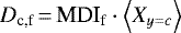 (2)
(2)
denotes for each cluster c the sensitivity of the classifier on feature f. Here, Xy=c are the scaled training data with labels y corresponding to cluster c. Figure 8 illustrates all cluster-specific mean decision boundaries. Dc,f quantifies the sensitivity on a parameter by its magnitude, as well as the orientation of the decision boundary by its sign. For example, the large negative value of cluster 4 in astart means that these planets prefer small initial orbital distances and their correct classification is very sensitive on this feature.
In the lower panels of Fig. 8, we plot all input features against the resulting planet mass at 5 Gyr, which is a proxy for cluster affiliation. Most planet clusters are especially sensitive on the initial orbital distance of the planetary embryo astart. Planets with masses higher than ~10 M⊕ are also very sensitive on the solid mass Msolid,0 and slightly sensitive on Mgas,0. The disk lifetime tdisk shows a weak correlation with planet mass and plays only a subordinate role.
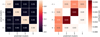 |
Fig. 6 Confusion of planet classifications. Left: confusion matrix from five-fold cross-validation. Rows are the actual clusters andcolumns are the predicted clusters. All clusters are classified with more than 95% accuracy. Right: same, but correct classifications removed to emphasize errors. Most misclassifications occur between clusters 2 and 3, which correspond to icy cores and giant planets. |
 |
Fig. 7 Pairwise relationships between all disk parameters, sorted by cluster affiliation. For 5000 randomly sampled planets in the population, each parameter is plotted against every other parameter while the color defines the planet’s cluster. The diagonal panels show the univariate distributions of the respective parameters, again colored by cluster assignment. Planet species most clearly separate in astart − Msolid,0 space, and the formation of giant planets (yellow) requires large solid reservoirs and a narrow range of initial orbital distance. |
4.4 Differences between single and multi-planet systems
Mutual interactions between planets in the same system introduce a fair amount of stochasticity, and some features that stood out in the single-planet population are smeared out in the multi-planet case. One example is the bimodal distribution of planet radii in the observed exoplanet sample (Fulton et al. 2017; Fulton & Petigura 2018; Hsu et al. 2018; Van Eylen et al. 2018; Mordasini 2020), which was theoretically predicted to be caused by photoevaporation of planetary envelopes by high-energy radiation from their host star (Jin et al. 2014; Owen & Wu 2013; Lopez & Fortney 2013). Other mechanisms have been proposed to produce this “radius valley” at roughly 2 R⊕ as well, including atmospheric loss due to internal heat from cooling planetary cores (Ginzburg et al. 2016, 2018; Gupta & Schlichting 2019), impacts of planetesimals (Wyatt et al. 2019) or other protoplanets (Liu et al. 2015), different internal compositions of planets residing above or below the valley (Zeng et al. 2019; Venturini et al. 2020), and atmospheric stripping by external radiation sources in stellar cluster environments (Kruijssen et al. 2020). In the Generation III Bern Model, photoevaporation by the host star and collisional stripping are taken into account.
The upper panels of Fig. 9 show the radius distributions of planets on close orbits (P < 80 d) in the single and multi-planet populations, respectively. Overplotted are occurrence rates derived from the Kepler mission in Hsu et al. (2019), which we marginalized over the period range 0 d to 80 d. The propagated uncertainties are indicated by vertical bars, and arrows mark upper limits. In our single-planet population, the evaporation valley is much less pronounced in this marginalized radius distribution than in radius-orbital distance space, where it shows a steep negative slope (compare Fig. 2). This highlights the importance of characterizing such demographic features in multiple dimensions. Compared to the observed valley at ~ 2 R⊕ (e.g., Fulton et al. 2017; Hsu et al. 2019), the synthetic one is shifted to larger radii. As has been shown in Jin & Mordasini (2018), this is due to atmosphere-less, icy cores that migrated inward from regions beyond the water ice line. This population is included in the planet cluster representing Neptunes, since the clustering algorithm mainly discriminated between (super-)Earths and Neptunes as rocky and icy planets, respectively.
In the multi-planet population, this is not the case. Here, the different clusters divide close-in planets into bare cores and planets with H/He envelopes, and the emerging radius valley separates the (super-)Earths and Neptunes clusters. Again, the valley is shifted to around 3 R⊕. Compared to the single-planet case, the slope of the valley in radius-orbital distance is less pronounced, which makes it appear deeper in the one-dimensional radius histogram. Future work within this series will address the synthetic radius valley in a more thorough manner (Mishra et al. 2021).
Other differences between the single and multi-planet populations can be seen in their period distributions (lower panels of Fig. 9). In the single-planet case, the combined contributions from (super-)Earths and Neptunes lead to a multimodal period distribution. On the other hand, the multi-planet population shows a continuous slope. In the range where Hsu et al. (2019) provide reliable occurrence estimates, this slope matches the observed one well. Causes for the difference between the single- and multi-planet case are the displacement of planets in semi-major axis due to gravitational encounters, a lack of close-in “failed cores” due to the high likelihood of such encounters on short orbits, and trapping of planets in resonant chains. In addition, mixed planetary compositions occur as a consequence of merger events. This places the planets into a continuum of bulk densities.
Regardless of this “stochastic processing” of the planets, we attempted to predict their clusters from initial conditions using the same features as in the single-planet case and following the procedure described in Sects. 4.1 to 4.2. Similar to before, keeping only planets that the GMM assigned to a specific cluster with a probability > 0.99 reduces the set to 21,761 planets. The randomly drawn training set comprising 80% of the data contains between 252 (giant planets) and 10 367 (icy cores) planets per cluster. A balanced random forest we trained on this set achieved an accuracy of 89% based on five-fold cross-validation. The other 4353 systems, which we left out as a test set, are predicted with 86% accuracy.
Similar to Fig. 6, Fig. 10 shows the confusion matrix of a random forest predicting the planet clusters in the multi-planet population. The ability to predict planet clusters from initial conditions varies across different planet types, with icy cores and giant planets being the most robust species. It can be seen that clusters 1 (Neptunes) and 4 ((super-)Earths), which occupy similar mass ranges, are affected by confusion the most. This is mainly due to the lack of (super-)Earths ≲ 0.1 M⊕ in the multi-planet case, where they typically fall victim to giant collisions with other planets. Neptunes are frequently mistaken as icy Earths and (super-)Earths are frequently confused to be Neptunes. These three groups of intermediate-mass planets share a similar domain in parameter space.
Figure 11 shows the positions of the planets in the multi-planet population in disk property space. Again, the different clusters differentiate the most in solid disk mass and initial orbital separation. Compared to the single-planet case, the separation of the clusters is less clean. The additional cluster identified in NG76, “icy Earths”, share a lot of parameter space with other planet types.
Using the mean decision boundary defined above (Eq. (2)), the dependence of different planet clusters on specific initial conditions can be visualized also for the multi-planet population (Fig. 12). The relationships largely copy those of the single-planet case: the starting location of the planet embryo shows the largest decision boundary amplitudes and differences among the clusters, and giant planets retain their distinct dependence on high solid and gas reservoirs.
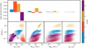 |
Fig. 8 Relation between disk features and planet species. Upper panel: mean decision boundaries of the classifier, indicating the importance of each feature and its preferred magnitude for the different clusters. The starting location of the planet embryo astart shows the largest variance in decision boundary. Giant planets (yellow) are also very sensitive on Msolid,0 and somewhat sensitive on Mgas,0. Lower panels: relationship of the input features with planet mass. The starting location of the planet embryo astart shows the strongest correlation with cluster affiliation and planet mass. |
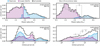 |
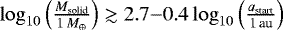
Fig. 9 Radius and period distributions of Neptunes and (super-)Earths. The contributions by Neptunes and (super-)Earths are shown in blue and purple, respectively. Upper panels: planet radius distribution for planets with periods P < 80 d. In the single-planet case (left), a population of migrated, icy cores in the Neptunes cluster shifts the synthetic radius valley to larger radii. In the case of multiple planets per system (right), the minimum in the distribution separates (super-)Earths and Neptunes. Compared to observed occurrence rates from Kepler (Hsu et al. 2019, gray), this minimum is shifted toward larger radii. Lower panels: period distributions of planets ≥ 1 R⊕. While the single-planet population (left) shows a multi-modal distribution, the multi-planet population has a continuous slope similar to observed occurrence rates. We note the different normalizations of synthetic and observed planets. |
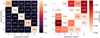 |
Fig. 10 Confusion of cluster classifications for a multi-planet population with N-body interactions. Same as Fig. 6, but computed for a population with 100 planets per disk that interact gravitationally. Clusters 2 (icy cores) and 3 (giant planets) are predicted most reliably. Due to giant collisions the classifier cannot predict, the super-Earths in cluster 4 are often mistaken for (sub-)Neptunes (cluster 1). |
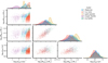 |
Fig. 11 Pairwise relationships between all disk parameters, sorted by cluster affiliation. Same as Fig. 7, but for a multi-planet population with N-body interactions.The separation of clusters is less pronounced than in the single-planet case. |
5 Discussion
5.1 Determining factors for the planet type
By predicting a planet’s cluster from a set of initial conditions of our planet formation model, we were able to establish links between properties of the protoplanetary disk and the corresponding planets (see Sect. 4.3.2). These links can be elucidated by using the planet mass MP as a proxy for the planet cluster and relating it to disk features (see Fig. 8). The feature with by far the highest predictive power is the starting location of the emerging protoplanetary embryo astart, which is expected in a core accretion scenario: an embryo at small orbital distance has only a small feeding zone from which it can accrete and thus it will remain small. At very large orbital distance, the dynamical and growth timescales are very large and the disk will have disappeared before a protoplanet can gain significant mass (Lissauer 1987, 1993; Kokubo & Ida 2002; Mordasini et al. 2009). Exactly at what orbital separations efficient planet growth is possible further depends on the amount, size, mass, and aerodynamic properties of planetesimals available there, and thus on the solid disk mass Msolid,0 (see below for a more detailed discussion on the interplay between orbital distance and local planetesimal density). As can be seen in the lower left panel of Fig. 8, intermediate orbits provide the best conditions for rapid growth. These trends are responsible for the clear separation of planet clusters in the astart-MP plane. Very small or very large initial orbital separations always lead to “failed cores" (low-mass instances of clusters 2 and 4). Short-period terrestrial planets and super-Earths (cluster 4) start on small orbits less than 1 au. (sub-)Neptunes (cluster 1) require intermediate orbits of roughly 0.5 au to 10 au. Finally, giant planets (cluster 3) start on distant orbits (≳3 au).
Other initial parameters show rather diverse importances that depend on the planet type. The mean decision boundaries (Eq. (2)) of Msolid,0 and Mgas,0 are close to zero for all clusters except giant planets, implying a small feature importance of these parameters for most planet types. While these two parameters are correlated in our model, which could in principle spuriously decrease their MDI, their relation to MP (lower panels of Fig. 8) reveals indeed only a weak relation to planet type. The picture differs for giant planets, which only form in disks that are rich both in gas (Mgas,0 ≳ 0.04 M⊙) and solids (Msolid,0 ≳ 200 M⊕). Given a specific starting location of its core, the efficiency of giant planet formation is strongly governed by Msolid, 0. The reason is this parameter’s direct relation to the local planetesimal density in the disk and thus a protoplanet’s ability to reach a core mass sufficient for runaway gas accretion. Lastly, the disk lifetime stipulates the time within which planet formation has to conclude. Surprisingly, this parameter shows close to no correlation with the resulting planet type. This shows that most disks provide material long enough (median ≈ 3.4 Myr) to complete planet formation. Within the scope of our model, early disk dispersal is not the preferred pathway to halt planet formation at low and intermediate masses.
We conclude that the occurrence of a certain type of planet is fundamentally related to disk properties, and it depends in particular on the orbital distance where the planetary embryo forms. Currently, we treat this important parameter as a Monte Carlo variable that is distributed based on simple theoretical arguments (Kokubo & Ida 2000). This is a major shortcoming of our formation model and our findings highlight the importance of a consistent treatment of planetary embryo formation (Voelkel et al. 2021a,b). Another effect we neglected thus far are the gravitational interactions between planets. We address this aspect below by discussing simulations done with the same model but multiple forming planets per disk (see Sect. 5.4). Future studies should also take into account the effects of pebble accretion (Ormel & Klahr 2010; Lambrechts & Johansen 2012), which influence the efficiency of solid accretion and may lead to a global redistribution of solid material in protoplanetary disks (e.g., Lambrechts & Johansen 2014; Morbidelli et al. 2015; Ormel et al. 2017; Bitsch et al. 2019).
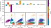 |
Fig. 12 Relation between disk features and planet species. Same as Fig. 8, but for a multi-planet population with N-body interactions. As in the single-planet case, the starting location of the planet embryo astart shows the largest variance in decision boundary. Giant planets (yellow) form only at high Msolid,0 and sufficient Mgas,0. |
5.2 Disk mass and embryo distance as predictors for planet type
Now that we have identified the solid disk mass and the initial orbital separation of a planetary embryo as the most important features, we investigate the regions that different planet types occupy in the space that these parameters span. Figure 7 shows distinct borders between the different clusters that can be explained by the combination of processes our planet formation model covers. The diagonal border between cluster 1 planets, which correspond to icy and atmosphere-bearing “Neptunes” on close and intermediate orbits, and cluster 4 planets, which are dry (super-)Earths, is shaped by photoevaporation of planetary envelopes: We recall that the clustering algorithm made the separation between these clusters mainly in RP, which leads to a completely atmosphere-less (super-)Earth cluster and a cluster of Neptunes that predominantly bear H/He envelopes. However, close to all (super-)Earths initially held an envelope that they subsequently lost due to photoevaporation, a fate that the more massive Neptunes were spared. Thus, the more solid material is available at a specific orbital distance, the more likely planets will grow massive enough to retain their atmospheres in the long term. The efficiency of photoevaporation is further a function of orbital distance, leading to the negative slope of the border between clusters 1 and 4 in astart − Msolid,0 (Jin & Mordasini 2018). Cluster 2 (“icy cores”) contains only terrestrial planets and failed cores with high amounts of volatile species and no atmospheres. They formed on distant orbits where the growth timescale is large, preventing them from growing beyond terrestrial size within the lifetime of the protoplanetary disk (Kokubo & Ida 2000).
5.3 Oligarchic growth of giant planets
The giant planets (cluster 3) in our planet population occupy a distinct region at large starting positions and high solid disk masses (see Fig. 7). It abruptly cuts off around 4 au, which corresponds to typical water ice line positions at accretion time (Burn et al. 2019). Here, the solid surface density jumps by a factor of four (Mordasini et al. 2012a), and significantly higher total solid disk masses are required to reach runaway gas accretion interior of this orbit. We therefore only considered planets beyond 4 au when we characterized the shape of the giant planet cluster. We did so by determining the hyperplanes in astart − Msolid,0 space that best separate these planets from other species. A Support Vector Machine (SVM, Cortes & Vapnik 1995) maximizes the distance of this plane to planets that belong to the “giant planets” cluster and all those that do not. We used the implementation in scikit-learn (Pedregosa et al. 2011) with a linear kernel and otherwise default hyperparameters, and trained the SVM on the full population. As in logarithmic representation the giant planet cluster has a triangular shape, we can approximate its border by a broken power law. Setting y = log10(Msolid) and x = log10(astart), we fit the piecewise linear function
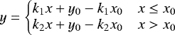 (3)
(3)
to separation functions found by the SVM. The best-fit values for these parameters are listed in Table 3. We calculated their uncertainties by the bootstrapping method: We repeatedly drew N random planets with replacement, where N is the total number of planets in our synthetic planet population, and trained the SVM on each of 1000 samples generated this way. In Fig. 13, we overlay the so found giant planet boundary onto the planets in astart − Msolid,0 space. Generally, giant planets formwhen 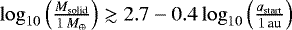 for cores emerging within ~10 au and when
 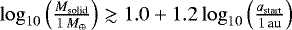 for cores emerging beyond. We point out that this result is only valid in the context of the assumptions of our model. Plausible limitations that might have influenced this outcome are the assumptions of a single population of planetesimals of the same size and efficientembryo formation throughout the disk, the non-consideration of pebble accretion (Ormel & Klahr 2010), and the largely featureless numerical disk that does not allow for “planet traps” (Chambers 2009). Another probable source of error is the omission of gravitational interactions between planets in the same system – the giant planet domain shifts moderately and is more diffuse when multiple concurrently forming planets are assumed (see Sect. 5.4). Nevertheless, we focus here on typical outcomes of isolated protoplanets since it allows a more quantitative assessment.
We also compared this boundary to characteristic parameters for planetesimal accretion in the oligarchic growth regime: the planetesimal isolation mass Miso and the growth timescale τgrow (e.g., Kokubo & Ida 2000; Raymond et al. 2014). On intermediate orbits of a few au, planetary growth is limited by the amount of material that can be accreted. Miso is a useful concept to quantify the maximum attainable core mass given this limit. On the other hand, τgrow gives an estimate for the time needed to reach a certain core mass, and sets the limit for wider orbits. For comparison with the giant planet cluster, we computed the local planetesimal densities corresponding to specific values of Miso and τgrow and translated them into total planetesimal disk masses Msolid,0. See Appendix B for derivations of these quantities.
Since our model includes planet migration, planets can accrete solid material beyond their planetesimal isolation mass by moving through the disk. Nevertheless, Miso is a proxy for how much can be accreted at a specific orbital distance and it is instructive to compare the shape of the giant planet population in astart − Msolid,0 space with the borders between planet clusters. In Fig. 13, we overplot isolines of disk solid masses necessary to reach different planetesimal isolation masses as a function of orbital separation (dashed blue lines). The lower border of the giant planet cluster matches well the slope of these lines. This indicates that in intermediate-mass disks with a few hundreds of M⊕ in solids, giant planet formation is limited by the protoplanets reaching Miso, that is, by clearing their feeding zone from solid material. We caution that the proximity of this border to the Miso = 5 M⊕ isoline does not imply that runaway gas accretion has set in at this mass, as planet migration results in a larger effective feeding zone (Alibert et al. 2005).
Beyond ~10 au, the border of the cluster matches the slope of isolines for different growth timescales. At these larger orbital distances, τgrow can reach the order of Myr for low planetesimal surface densities and thus becomes comparable to the lifetime of the protoplanetary disk. In this regime, the growth of a planetary core is limited by the time available to accrete the planetesimals in the domain of a planet’s orbit. As can be seen in the plot, the Msolid,0(a) isoline where the growth timescale corresponds to the median of the disk lifetime, τgrow ≈ 3.4 Myr, is a good fit to the border between giant planets (yellow) and icy cores (red). Indeed, most of the giant planets close to this threshold formed in long-lived disks (see Fig. B.1). This indicates that for planetesimal densities just sufficient for the formation of massive cores, entering runaway gas accretion depends on the longevity of the host disk.
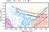 |
Fig. 13 Clusters of planets in astart − Msolid,0 space of their nascent protoplanetary disk. The green line is the hyperplane that best separates the giant planet cluster (yellow markers) from the other planets and was obtained by training a Support Vector Machine (SVM). Closeby gray lines show random draws from bootstrap sampling and illustrate the uncertainties. We overplot isolines of planetesimal masses needed to reach specific core masses (blue dashed lines), as well as isolines corresponding to specific growth timescales for reaching a core mass of 10 M⊕ (green dashed lines). Their slopes are similar to the SVM fit that encloses the giant planets, indicating that the onset of runaway growth is limited by the locally available planetesimal mass and by the disk lifetime. |
5.4 The influence of N-body interactions
Our cluster analysis and prediction from initial conditions has shown that even in the case of multi-planet systems with gravitational interactions, most of the links between disk and planet properties remain intact (see Sect. 4.4). Still, the demographic structures in the multi-planet population are somewhat smeared out compared to the single-planet case, and the strength of this effect is different for individual clusters. We have seen that (super-)Earths and Neptunes are affected the most by this sort of mixing. These planet types cannot be reliably predicted from disk properties if N-body interactions are taken into account. Interestingly, the confusion is asymmetric: Planets predicted as Neptunes often become (super-)Earths, while those predicted as (super-)Earths rarely become Neptunes. The reason is something the classifier cannot predict: The misclassified (super-)Earths are typically planets that got stripped of their atmospheres in giant collisions with other planets. From this follows that our model would produce too many Neptunes if such collisions are not taken into account (as is the case in single-planet simulations). This highlights the need for global planet formation models to include a consistent treatment of N-body interactions and giant impacts, as has already been suggested by Alibert et al. (2013) and in Paper I.
Another difference compared to the single-planet case is that close-in planets with small radii and masses are strongly depleted. This is because they often undergo giant collisions and merge into more massive bodies. The resulting lack of “sub-Earths” provides an interesting prediction for future planet searches that will push beyond the current mass and radius limits. Whether a multitude or a desert of such planets will be found could give valuable clues to the prevalence of planetary collisions.
6 Conclusions
We have investigated how different properties of protoplanetary disks relate to the emergence of different planet types in a planetesimal-based core accretion context. By performing a cluster analysis on synthetic planet populations from a global model of planet formation and evolution, we identified clusters of planets in a parameter space of typical exoplanet observables. We examined how well these clusters can be predicted from disk properties and studied the dependencies of different planet types. Our main conclusions are:
Planets form distinct groups in {a, MP, RP} space, especially when dynamical interactions within multi-planet systems are neglected. Without presupposing planet types or their number, we identified four clusters corresponding to (sub-)Neptunes, icy cores, giant planets, and (super-)Earths.
These groups differentiate within the first 0.1 Myr of the formation process and show correlations with properties of their host disks. Such associations between disk and planet properties enable the prediction of planet species to high accuracy (98% in the single-planet case and 89% in the multi-planet case).
The most important predictor for planet clusters is the orbital position of the emerging planetary core, followed by the solid mass available in the disk. The disk lifetime plays a subordinate role, but can be a limiting factor for threshold values of the above mentioned parameters.
The position of giant planets in disk parameter space can be associated with known characteristics of oligarchic planetesimal accretion: For limited available amounts of solid material and within ~10 au, core growth is limited by planetesimal isolation and giant planets form when
 . On more distant orbits, core accretion is limited by the growth timescale and giants emerge when
 .
.When multiple planets form and interact in the same system, for most planet types the associations between disk properties and planet properties remain. However, planets on track to become sub-Neptunes often lose their atmospheres in giant collisions and turn into super-Earths, which impedes predictions for this planet type.
Overall, we have shown that synthetic planet populations from state-of-the-art core accretion models largely mirror the planet types recognized by exoplanet demographics. Our results highlight the importance of N-body integrations in global planet formation models that aim for reliable predictions in the domain of low-mass planets. Beyond that, constraining the orbital distances at which planetary cores form is of major relevance for the full range of planet types. Population syntheses of the next generation should recognize this by including self-consistent treatments of planetary embryo formation.
Acknowledgements
The authors thank Gabriele Pichierri for fruitful discussions. We thank the anonymous referee for valuable comments that improved the manuscript. This work was supported by the DFG Research Unit FOR2544 “Blue Planets around Red Stars”, project no. RE 2694/4-1. T.H. acknowledges support from the European Research Council under the Horizon 2020 Framework Program via the ERC Advanced Grant Origins 83 24 28. This research was supported by the Deutsche Forschungsgemeinschaft through the Major Research Instrumentation Programme and Research Unit FOR2544 “Blue Planets around Red Stars” for T.H. under contract DFG He 1935/27-1 and for H.K. under contract DFG KL1469/15-1. Parts of this work has been carried out within the framework of the National Centre for Competence in Research PlanetS funded by the Swiss National Science Foundation (SNSF). R.B. and Y.A. acknowledge financial support from the SNSF under grant 200020_172746. Some of the computations have been carried out on the DRACO cluster of the Max Planck Society, which is hosted at the Max Planck Computing and Data Facility in Garching (Germany).
Appendix A The choice of a clustering algorithm
A.1 Clustering algorithms
For the cluster analysis in Sect. 3, we examined several other clustering algorithms in addition to GMM2 and explored their behavior on our data set. For each method, we used its implementation in scikit-learn (Pedregosa et al. 2011) and, where applicable, chose the default Euclidean distance metric. The algorithms considered are centroid, density, or hierarchical-based. A centroid-based method we explored was K-means (MacQueen 1967; Lloyd 1982). In the density-based group, we tested DBSCAN and OPTICS (Ester et al. 1996; Ankerst et al. 1999). For hierarchical clustering, we examined Agglomerative clustering (Ward 1963) besides GMM (McLachlan 1988).
K-Means3 (MacQueen 1967; Lloyd 1982) is a centroid-based clustering algorithm: It randomly initializes k centroids and associates each data point to the centroid that is closest to it, then shifts the centroids to the mean of their cluster. These steps are repeated until no changes occur. The algorithm requires only a single hyperparameter k, which is the number of clusters.
Agglomerative clustering4 (Ward 1963) is a bottom-up hierarchical clustering algorithm: Each data point begins as its own cluster and incrementally merges similar pairs of clusters into a new cluster. This process is repeated until there are k clusters left, where k is the hyperparameter for the number of clusters. When testing this algorithm, we used a hyperparameter called linkage to quantify similarity between pairs of clusters (e.g., Ward 1963; Szekely & Rizzo 2005). Empirically, we found that the “Ward” linkage is optimal.
DBSCAN5 (Ester et al. 1996)is a density-based clustering algorithm classifying each data point as either a core point (with at least minPts neighboring points within a distance ϵ), a reachable point (that is within distance ϵ of the core point), or an outlier (that is not reachable by any core point). All core points and their reachable points form a cluster, but outliers do not. The method we tested is an advancement of DBSCAN with improved performance on data sets of varying density. This method called OPTICS6 (Ankerst et al. 1999)has one hyperparameter: minPts – the minimum number of points nearby to make a core point.
A.2 Validation metrics and choice of method
Each of these methods has hyperparameters, that is, parameters that are not derived during model training but that control the learning process itself. We used a number of validation metrics to quantify the clustering performance for each method and specific choice of hyperparameters. Some of these metrics are method-specific and can only be used with a specific algorithm. These are the elbow method (e.g., Thorndike 1953; Ketchen & Shook 1996), the Bayesian and Aikake Information Criterions (BIC and AIC, e.g., Akaike 1973; Schwarz 1978; Cavanaugh & Neath 2019), and the dendrogram method (e.g., Nielsen 2016). The elbow method is used to evaluate the performance of the K-Means algorithm. By plotting the within-cluster sum-of-squares against k, an “elbow”-shaped curve emerges. The ideal k will be one close to the elbow. The reasoning for this is that we aim to find the first k that minimizes the within-cluster sum-of-squares. BIC and AIC are used for GMM. Both are based on information theory and are used to prevent overfitting and underfitting to choose the most optimized model. The dendrogram method is used to judge the bottom-up process of Agglomerative clustering. It shows the clustering at each hierarchy, where the y-axis is the distance between clusters and the x-axis shows the clusters. Therefore, the goal is to perform a horizontal cut such that the vertical distance is maximized. As one traverses up the hierarchy, the vertical distance naturally increases.
In addition to these scores, we used the following scalar-valued metrics that can be used for any method: the Silhouette score (Rousseeuw 1987), the CaliÅski–arabasz score (CH, Caliñski & Harabasz 1974), and the Davies–Bouldin score (DB, Davies & Bouldin 1979). The Silhouette score is computed from the mean intra-cluster distance and the mean nearest-cluster distance. Silhouette scores range between −1 and 1 with 1 being the best and −1 being the worst, and values near 0 implying overlapping clusters. We aimed to maximize this score. The Cali?ski–Harabasz score is the ratio of the within-cluster dispersion and the between-cluster dispersion, where dispersion is the sum of the squared distances. Again, we aimed to maximize this score. The Davies-Bouldin score determines the clustering performance by using the ratio of the within-cluster distances to the between-cluster distances. As a result, compact clusters that are far apart give better scores. The minimum score is 0, and we aimed to minimize this score.
A.3 Model selection
Our approach in selecting the best clustering method was as follows: First, we applied each method to the {a, MP, RP} subspace of the NG73 planet population for a wide range of hyperparameters. We then compared the validation metrics computed for the resulting clusterings. The scores did not always agree unanimously, which is expected, as the structures in our multidimensional data set are rather complex and the scores consider different goals regarding an optimal clustering. The next step was thus to produce, for each combination of method and hyperparameters, scatter plots that showed the clustering results in different projections of {a, MP, RP} space. Using these plots, we could compare the different partitionings and determine the most sensible model. Figure A.1 shows these diagnostic plots for k-means, OPTICS, and Agglomerative clustering, using the choice of hyperparameters considered most appropriate. The diagnostic plots for GMM are shown in Fig. A.2. Based on this selection procedure, GMM showed the best performance and we considered it our nominal method for clustering.
A free parameter of GMMs is the number of components N, which we chose using the same two-step approach as in the method selection. After the validation metrics suggested N = 4, N = 6 for NG73 and N = 3, N = 5 for NG76 (see Fig. 1), we assessed the diagnostic plots shown in Fig. A.2. For NG73, we found that the GMM with N = 6 reaches similar scores than N = 4 but traces less reliably the underdensities in the domain and partly draws cluster borders through rather arbitrary regions. We thus chose the GMM with N = 4 as our nominal model for the single-planet case. For NG76, the model with more components reliably detects visible overdensities and outperforms the less complex model. Hence, we adopted the GMM with N = 5 as the nominal model for the multi-planet case.
 |
Fig. A.1 Diagnostic plots for clustering method selection. For each alternative clustering algorithm we explored, we show the validation metrics we used to choose hyperparameters. Based on these metrics, we show the resulting clustering for the most promising choices in the corner plots. (a) Even in the best case (N = 5), k-means’ approach to draw cluster borders is too simplistic to account for the structure in our data. (b) For the numerically best choice of minPts, OPTICS finds three clusters of extremely different sizes. Most of the data belong to a single cluster that covers the whole domain, and no sensible relation to the data point density is apparent. (c) Agglomerative clustering suggests the existence of five clusters. Again, no reasonable partitioning is visible. The lower right panel shows the dendrogram corresponding to this clustering. |
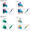 |
Fig. A.2 Diagnostic plots for GMM clustering model selection. According to our validation metrics, the best candidate number of clusters are N = 4, N = 6 for NG73 and N = 3, N = 5 for NG76 (compare Fig. 1). Panels a–d: show the clustering results of these choices. The models in a) (N = 4) and d) (N = 5) trace the over- and underdensities in the domain best and we consider them our nominal models. |
Appendix B Boundary conditions for giant planet formation
B.1 Derivation of isolation mass and growth timescale
In Sect. 5.3, we characterize the cluster of giant planets in astart − Msolid,0 space, where it occupies a distinct triangular region. In the following, we derive two quantities that shape this region: the total solid disk mass as a function of orbital distance for different planetesimal isolation masses and for different growth timescales.
Miso gives the mass in planetesimals a protoplanet can accrete given a feeding zone of width b ≃ 10rH, where 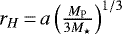 . Then,
 (B.1)
(B.1)
where Σsolid is the planetesimal surface density. Setting the planetary mass to the planetesimal isolation mass, MP ≡ Miso, yields
 (B.2)
(B.2)
To get an estimate on which initial solid mass content is required to reach a certain isolation mass, we express this as
 (B.3)
(B.3)
For the power law disk profile used in our model (Andrews et al. 2009),
![Mathematical equation: \begin{equation*} \Sigma(r)\,{=}\,\Sigma_0 \left(\frac{r}{r_0}\right)^{-\beta} \exp \left[- \left(\frac{r}{r_{\textrm{cut,g}}}\right)^{(2-\beta)}\right], \end{equation*}](/articles/aa/full_html/2021/12/aa40551-21/aa40551-21-eq13.png) (B.4)
(B.4)
we consider the outer disk radii rcut,g and rcut,s for the gas and solid disk, respectively. The radial slope of Σsolid is characterized by the power law index β, and Σ0 is the surface density at a reference orbital distance r0 = 5.2 au. Then, the total mass of the planetesimal disk is
 (B.5)
(B.5)
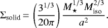
where rcut,s = 0.5rcut,g (following findings from dust disk observations, Ansdell et al. 2018) and β = 1.5 (motivated by planetesimal formation models, Lenz et al. 2019). Substituting Eq. (B.3) into Eq. (B.5), the total solid mass required to reach Miso is given by
![Mathematical equation: \begin{equation*} M_{\textrm{solid}} (M_{\textrm{P}}\,{=}\,M_{\textrm{iso}})\,{=}\,\frac{3^{1/3}}{10} \frac{r_{\textrm{cut,s}}^{2-\beta}}{2-\beta} \frac{M_{\star}^{1/3} M_{\textrm{iso}}^{2/3}}{a^{2-\beta}} \exp \left[-\left(\frac{a}{r_{\textrm{cut,s}}}\right)^{2 - \beta} \right]^{-1}. \end{equation*}](/articles/aa/full_html/2021/12/aa40551-21/aa40551-21-eq15.png) (B.6)
(B.6)
Similarly, we can derive the solid disk mass needed to reach a specific mass in the outer disk regions, where growth is mainly limited by the growth timescale τgrow. For the oligarchic growth regime (Ida & Makino 1993), this timescale can be approximated by
![Mathematical equation: \begin{equation*}\begin{split} \tau_{\textrm{grow}} \approx & 1.2 \,{\times}\,10^{5} \mathrm{yr}\left(\frac{\Sigma_{\mathrm{p}}}{10 \mathrm{~g} \mathrm{~cm}^{-2}}\right)^{-1}\left(\frac{a}{1 \mathrm{au}}\right)^{1 / 2}\left(\frac{M_{\textrm{c}}}{M_{\oplus}}\right)^{1 / 3}\left(\frac{M_{\star}}{M_{\odot}}\right)^{-1 / 6} \\ & {\times}\,\left[\left(\frac{\Sigma_{\mathrm{g}}}{2400 \mathrm{~g} \mathrm{~cm}^{-2}}\right)^{-1 / 5}\left(\frac{a}{1 \mathrm{au}}\right)^{1 / 20}\left(\frac{M_{\textrm{pla}}}{10^{18} \mathrm{~g}}\right)^{1 / 15}\right]^{2} \end{split} \end{equation*}](/articles/aa/full_html/2021/12/aa40551-21/aa40551-21-eq16.png) (B.7)
(B.7)
(Mordasini 2018). Solving for Σp and substituting into Eq. (B.5) gives
![Mathematical equation: \begin{eqnarray*} && M_{\textrm{solid}}(a, \tau_{\textrm{grow}})\,{=}\, {7.54}\,\textrm{g\,cm}^{-2} \frac{r_0^{\beta} r_{\textrm{cut,s}}^{2 - \beta}}{2 - \beta} \left(\frac{M_{\textrm{c}}}{M_{\oplus}}\right)^{1 / 3} \left(\frac{M_{\star}}{M_{\odot}}\right)^{-1/6}\nonumber\\ &&\quad {\times}\,\left[\left(\frac{\Sigma_{\mathrm{g}}(a)}{2400 \mathrm{~g} \mathrm{~cm}^{-2}}\right)^{-1 / 5}\left(\frac{M_{\textrm{pla}}}{10^{18} \mathrm{~g}}\right)^{1 / 15}\right]^{2} \left(\frac{\tau_{\textrm{grow}}}{{1}\,\textrm{Myr}} \right)^{-1} \left(\frac{a}{1 \mathrm{au}}\right)^{3/5},\nonumber\\ \end{eqnarray*}](/articles/aa/full_html/2021/12/aa40551-21/aa40551-21-eq17.png) (B.8)
(B.8)
where Σg was computed using the population-wide median of the reference surface density Σ0,gas. For the cutoff radii of the gas and solid disk, we proceeded in the same way and assumed the population median, respectively. For the planetesimal mass Mpla, we assumed a density of 1 g cm−2, which results in Mpla = 1.13 × 10¹¹ kg for the planetesimals in our model (Emsenhuber et al. 2021a). We adopted a core mass Mc of 10 M⊕.
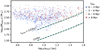 |
Fig. B.1 Planetesimal disk mass and initial planet core position of giant planets forming in disks of different lifetimes. Markers show the distribution of all planets classified as “cluster 3: giant planet” in astart −Msolid,0 space, color-coded by the lifetime of their nascent disk. We overplot isolines of planetesimal masses corresponding to specific growth timescales τgrow for reaching a core mass of 10 M⊕. Giant planet growth is limited by the disk lifetime, and the formation of giant planets far out requires high planetesimal masses and long lifetimes. |
B.2 Disk lifetime limits giant planet growth
Figure B.1 shows the cluster of giant planets in the space spanned by two important initial disk properties, astart and Msolid,0. The colors correspond to different lifetimes of the protoplanetary disk in which they formed. Most giants grow (and survive) in disks with lifetimes 3 Myr to 6 Myr. Only long-living disks enable formation of giant planets at low solid disk masses and large orbital distances. In short-lived disks, there is only a narrow region of embryo starting positions where giant planets grow at low planetesimal surface densities.
References
- Akaike, H. 1973, Proceedings of the 2nd International Symposium on Information Theory, 267 [Google Scholar]
- Alexander, R., Pascucci, I., Andrews, S., Armitage, P., & Cieza, L. 2014, Protostars and Planets VI, eds. H. Beuther, R. S. Klessen, C. P. Dullemond, & T. Henning (Tucson: University of Arizona Press), 475 [Google Scholar]
- Alibert, Y., Mordasini, C., Benz, W., & Winisdoerffer, C. 2005, A&A, 434, 343 [NASA ADS] [CrossRef] [EDP Sciences] [Google Scholar]
- Alibert, Y., Carron, F., Fortier, A., et al. 2013, A&A, 558, A1 [Google Scholar]
- Andrews, S. M., Wilner, D. J., Hughes, A. M., Qi, C., & Dullemond, C. P. 2009, ApJ, 700, 1502 [CrossRef] [Google Scholar]
- Andrews, S. M., Wilner, D. J., Hughes, A. M., Qi, C., & Dullemond, C. P. 2010, AJ, 723, 1241 [NASA ADS] [CrossRef] [Google Scholar]
- Ankerst, M., Breunig, M. M., Kriegel, H.-P., & Sander, J. 1999 SIGMOD ’99: Proceedings of the 1999 ACM SIGMOD international conference on Management of data, 49 [Google Scholar]
- Ansdell, M., Williams, J. P., Trapman, L., et al. 2018, Alma Survey of Lupus Protoplanetary Disks II: Gas Disk Radii [Google Scholar]
- Baraffe, I., Homeier, D., Allard, F., & Chabrier, G. 2015, A&A, 577, A42 [NASA ADS] [CrossRef] [EDP Sciences] [Google Scholar]
- Bitsch, B., & Johansen, A. 2017, in Formation, Evolution, and Dynamics of Young Solar Systems, eds. M. Pessah, & O. Gressel, 445, 339 [NASA ADS] [CrossRef] [Google Scholar]
- Bitsch, B., Lambrechts, M., & Johansen, A. 2015, A&A, 582, C2 [Google Scholar]
- Bitsch, B., Lambrechts, M., & Johansen, A. 2018, A&A, 609, C2 [NASA ADS] [CrossRef] [EDP Sciences] [Google Scholar]
- Bitsch, B., Izidoro, A., Johansen, A., et al. 2019, A&A 623, A88 [NASA ADS] [CrossRef] [EDP Sciences] [Google Scholar]
- Bodenheimer, P., & Pollack, J. B. 1986, Icarus, 67, 391 [Google Scholar]
- Bodenheimer, P., Hubickyj, O., & Lissauer, J. J. 2000, Icarus, 143, 2 [Google Scholar]
- Box, G. E. P., & Cox, D. R. 1964, J. R. Stat. Soc.: Ser. B (Methodological), 26, 211 [Google Scholar]
- Breiman, L. 1996, Mach. Learn., 24, 123 [Google Scholar]
- Breiman, L. 2001, Mach. Learn., 45, 5 [Google Scholar]
- Breiman, L., Friedman, J., Stone, C. J., & Olshen, R. A. 1984, Classification and Regression Trees, The Wadsworth Statistics/Probability Series (Monterey, CA: Wadsworth & Brooks/Cole Advanced Books & Software) [Google Scholar]
- Brewer, J. M., Wang, S., Fischer, D. A., & Foreman-Mackey, D. 2018, ApJ, 867, L3 [NASA ADS] [CrossRef] [Google Scholar]
- Bryan, M. L., Knutson, H. A., Lee, E. J., et al. 2019, ApJ, 157, 52 [CrossRef] [Google Scholar]
- Burn, R., Marboeuf, U., Alibert, Y., & Benz, W. 2019, A&A, 629, A64 [NASA ADS] [CrossRef] [EDP Sciences] [Google Scholar]
- Burn, R., Schlecker, M., Mordasini, C., et al. 2021, A&A, 656, A72 (Paper IV) [NASA ADS] [CrossRef] [EDP Sciences] [Google Scholar]
- Caliñski, T., & Harabasz, J. 1974, Commun. Stat., 3, 1 [Google Scholar]
- Cavanaugh, J. E., & Neath, A. A. 2019, Wiley Interdiscipl. Rev.: Comput. Stat., 11, e1460 [CrossRef] [Google Scholar]
- Chabrier, G., Baraffe, I., Leconte, J., Gallardo, J., & Barman, T. 2009 AIP Conf. Proc., 1094, 102 [NASA ADS] [CrossRef] [Google Scholar]
- Chambers, J. E. 1999, MNRAS, 304, 793 [Google Scholar]
- Chambers, J. 2006, Icarus, 180, 496 [NASA ADS] [CrossRef] [Google Scholar]
- Chambers, J. E. 2009, AJ, 705, 1206 [NASA ADS] [CrossRef] [Google Scholar]
- Chambers, J. 2018, ApJ, 865, 30 [Google Scholar]
- Chambers, J. E., Wetherill, G. W., & Boss, A. P. 1996, Icarus, 119, 261 [Google Scholar]
- Chaparro Molano, G., Bautista, F., Miguel, Y., et al. 2019, Proc. Int. Astron. Union, 152 [Google Scholar]
- Chen, C., Liaw, A., & Breiman, L. 2004, Research and Industry, 110, 24 [Google Scholar]
- Clarke, C. J., Gendrin, A., Sotomayor, M., et al. 2001, MNRAS, 328, 485 [NASA ADS] [CrossRef] [Google Scholar]
- Cortes, C., & Vapnik, V. 1995, Mach. Learn., 20, 273 [Google Scholar]
- D’Angelo, G., Kley, W., & Henning, T. 2003, ApJ, 586, 540 [Google Scholar]
- Davies, D. L., & Bouldin, D. W. 1979, IEEE Trans. Pattern Anal. Mach. Intell., PAMI-1, 224 [Google Scholar]
- Dittkrist, K. M., Mordasini, C., Klahr, H., Alibert, Y., & Henning, T. 2014, A&A, 567, A121 [NASA ADS] [CrossRef] [EDP Sciences] [Google Scholar]
- Dra̧zkowska, J., Alibert, Y., & Moore, B. 2016, A&A, 594, A105 [CrossRef] [EDP Sciences] [Google Scholar]
- Emsenhuber, A., Mordasini, C., Burn, R., et al. 2021a, A&A, 656, A69 (Paper I) [NASA ADS] [CrossRef] [EDP Sciences] [Google Scholar]
- Emsenhuber, A., Mordasini, C., Burn, R., et al. 2021b, A&A, 656, A70 (Paper II) [NASA ADS] [CrossRef] [EDP Sciences] [Google Scholar]
- Ester, M., Kriegel, H.-P., Sander, J., & Xu, X. 1996, KDD-96 Proceedings (AAAI Press), 226 [Google Scholar]
- Fernandes, R. B., Mulders, G. D., Pascucci, I., Mordasini, C., & Emsenhuber, A. 2019, ApJ, 874, 81 [NASA ADS] [CrossRef] [Google Scholar]
- Fortier, A., Alibert, Y., Carron, F., Benz, W., & Dittkrist, K. M. 2013, A&A, 549, A44 [NASA ADS] [CrossRef] [EDP Sciences] [Google Scholar]
- Fortney, J. J.,& Nettelmann, N. 2010, Space Sci. Rev., 152, 423 [CrossRef] [Google Scholar]
- Fressin, F., Torres, G., Charbonneau, D., et al. 2013, ApJ, 766, 81 [NASA ADS] [CrossRef] [Google Scholar]
- Fulton, B. J., & Petigura, E. A. 2018, AJ, 156, 264 [Google Scholar]
- Fulton, B. J., Petigura, E. A., Howard, A. W., et al. 2017, ApJ, 154, 109 [Google Scholar]
- Ginzburg, S., Schlichting, H. E., & Sari, R. 2016, ApJ, 825, 29 [Google Scholar]
- Ginzburg, S., Schlichting, H. E., & Sari, R. 2018, MNRAS, 476, 759 [Google Scholar]
- Goldreich, P., & Tremaine, S. 1979, ApJ, 233, 857 [Google Scholar]
- Guillot, T. 2005, Annu. Rev. Earth Planet. Sci., 33, 493 [Google Scholar]
- Gupta, A., & Schlichting, H. E. 2019, MNRAS, 487, 24 [Google Scholar]
- Hartley, H. O. 1958, Biometrics, 14, 174 [Google Scholar]
- He, M. Y., Ford, E. B., & Ragozzine, D. 2020, AJ, 17, 1 [Google Scholar]
- Ho, T. K. 1995, in Proceedings of 3rd International Conference on Document Analysis and Recognition, 1, 278 [Google Scholar]
- Ho, T. 1998, IEEE Trans. Pattern Anal. Mach. Intell., 20, 832 [Google Scholar]
- Hobson, M. J., & Gomez, M. 2017, New Astron., 55, 1 [CrossRef] [Google Scholar]
- Hollenbach, D., Johnstone, D., Lizano, S., & Shu, F. 1994, ApJ, 428, 654 [NASA ADS] [CrossRef] [Google Scholar]
- Howard, A. W., Marcy, G. W., Bryson, S. T., et al. 2012, ApJS, 201, 15 [Google Scholar]
- Hsu, D. C., Ford, E. B., Ragozzine, D., & Morehead, R. C. 2018, ApJ, 155, 205 [CrossRef] [Google Scholar]
- Hsu, D. C., Ford, E. B., Ragozzine, D., & Ashby, K. 2019, ApJ, 158, 109 [CrossRef] [Google Scholar]
- Hueso, R., & Guillot, T. 2005, A&A, 442, 703 [NASA ADS] [CrossRef] [EDP Sciences] [Google Scholar]
- Ida, S., & Lin, D. N. C. 2004a, ApJ, 604, 388 [Google Scholar]
- Ida, S., & Lin, D. N. C. 2004b, ApJ, 616, 567 [NASA ADS] [CrossRef] [Google Scholar]
- Ida, S., & Makino, J. 1993, Icarus, 106, 210 [NASA ADS] [CrossRef] [Google Scholar]
- Jain, A. K., & Dubes, R. C. 1988, Algorithms for Clustering Data [Google Scholar]
- Jin, S., & Mordasini, C. 2018, ApJ, 853, 163 [Google Scholar]
- Jin, S., Mordasini, C., Parmentier, V., et al. 2014, ApJ, 795, 65 [Google Scholar]
- Kawahara, H.,& Masuda, K. 2019, ApJ, 157, 218 [CrossRef] [Google Scholar]
- Keppler, M., Benisty, M., Müller, A., et al. 2018, A&A, 617, A44 [NASA ADS] [CrossRef] [EDP Sciences] [Google Scholar]
- Ketchen, D. J., & Shook, C. L. 1996, Strategic Manage. J., 17, 441 [CrossRef] [Google Scholar]
- King, G. W., & Wheatley, P. J. 2021, MNRAS, 501, L28 [Google Scholar]
- Kokubo, E., & Ida, S. 2000, Icarus, 143, 15 [Google Scholar]
- Kokubo, E., & Ida, S. 2002, ApJ, 581, 666 [Google Scholar]
- Kruijssen, J. M. D., Longmore, S. N., & Chevance, M. 2020, ApJ, 905, L18 [Google Scholar]
- Lambrechts, M., & Johansen, A. 2012, A&A, 544, A1 [Google Scholar]
- Lambrechts, M., & Johansen, A. 2014, A&A, 572, A107 [NASA ADS] [CrossRef] [EDP Sciences] [Google Scholar]
- Lammer, H., Selsis, F., Ribas, I., et al. 2003, ApJ, 598, L121 [Google Scholar]
- Lee, E. J., & Chiang, E. 2015, ApJ, 811, 41 [Google Scholar]
- Lemaître, G., Nogueira, F., & Aridas, C. K. 2017, J. Mach. Learn. Res., 18, 1 [Google Scholar]
- Lenz, C. T., Klahr, H., & Birnstiel, T. 2019, ApJ, 874, 36 [NASA ADS] [CrossRef] [Google Scholar]
- Lin, J. W., Lee, E. J., & Chiang, E. 2018, MNRAS, 480, 4338 [Google Scholar]
- Lissauer, J. J. 1987, Icarus, 69, 249 [NASA ADS] [CrossRef] [Google Scholar]
- Lissauer, J. J. 1993, ARA&A, 31, 129 [NASA ADS] [CrossRef] [Google Scholar]
- Liu, S. F., Hori, Y., Lin, D. N., & Asphaug, E. 2015, ApJ, 812, 164 [CrossRef] [Google Scholar]
- Lloyd, S. P. 1982, IEEE Trans. Inform. Theory, 28, 129 [CrossRef] [Google Scholar]
- Lodders, K. 2003, ApJ, 591, 1220 [Google Scholar]
- Lopez, E. D., & Fortney, J. J. 2013, ApJ, 776, 2 [Google Scholar]
- Lopez, E. D., Fortney, J. J., & Miller, N. 2012, ApJ, 761, 59 [Google Scholar]
- Lüst, R. 1952, Z. Natur. Teil A, 7, 87 [CrossRef] [Google Scholar]
- Lynden-Bell, D., & Pringle, J. E. 1974, MNRAS, 168, 603 [Google Scholar]
- MacQueen, J. 1967, in Proceedings of the Fifth Berkeley Symposium on Mathematical Statistics and Probability, 1: Statistics (Berkeley, Calif.: University of California Press), 281 [Google Scholar]
- McLachlan, G. 1988, Mixture Models : Inference and Applications to Clustering (New York, NY: M. Dekker) [Google Scholar]
- Miguel, Y., Cridland, A., Ormel, C. W., Fortney, J. J., & Ida, S. 2020, MNRAS, 491, 1998 [NASA ADS] [Google Scholar]
- Mishra, L., Alibert, Y., Leleu, A. 2021, A&A, 656, A74 (Paper VI) [NASA ADS] [CrossRef] [EDP Sciences] [Google Scholar]
- Mizuno, H. 1980, Progr. Theor. Phys., 64, 544 [CrossRef] [Google Scholar]
- Mizuno, H., Nakazawa, K., & Hayashi, C. 1978, Progr. Theor. Phys., 60, 699 [CrossRef] [Google Scholar]
- Morbidelli, A.,& Nesvorny, D. 2012, A&A, 546, A18 [NASA ADS] [CrossRef] [EDP Sciences] [Google Scholar]
- Morbidelli, A., Lambrechts, M., Jacobson, S., & Bitsch, B. 2015, Icarus, 258, 418 [NASA ADS] [CrossRef] [Google Scholar]
- Mordasini, C. 2018, in Handbook of Exoplanets (Cham: Springer International Publishing), 2425 [CrossRef] [Google Scholar]
- Mordasini, C. 2020, A&A, 638, A1 [Google Scholar]
- Mordasini, C., Alibert, Y., & Benz, W. 2009, A&A, 501, 1139 [CrossRef] [EDP Sciences] [Google Scholar]
- Mordasini, C., Alibert, Y., Benz, W., Klahr, H., & Henning, T. 2012a, A&A, 541, A1 [Google Scholar]
- Mordasini, C., Alibert, Y., Georgy, C., et al. 2012b, A&A, 547, A112 [NASA ADS] [CrossRef] [EDP Sciences] [Google Scholar]
- Mordasini, C. A., Alibert, Y., Klahr, H. H., & Henning, T. 2012c, A&A, 547, A111 [NASA ADS] [CrossRef] [EDP Sciences] [Google Scholar]
- Mulders, G. D., Pascucci, I., & Apai, D. 2015, ApJ, 814, 130 [NASA ADS] [CrossRef] [Google Scholar]
- Mulders, G. D., Pascucci, I., Apai, D., & Ciesla, F. J. 2018, ApJ, 156, 24 [CrossRef] [Google Scholar]
- Mulders, G. D., O’Brien, D. P., Ciesla, F. J., Apai, D., & Pascucci, I. 2020, ApJ, 897, 72 [NASA ADS] [CrossRef] [Google Scholar]
- Nakamoto, T., & Nakagawa, Y. 1994, ApJ, 421, 640 [Google Scholar]
- Ndugu, N., Bitsch, B., & Jurua, E. 2018, MNRAS, 474, 886 [Google Scholar]
- Nielsen, F. 2016, in Introduction to HPC with MPI for Data Science (Springer International Publishing), 195 [CrossRef] [Google Scholar]
- Ormel, C. W., & Klahr, H. H. 2010, A&A, 520, A43 [NASA ADS] [CrossRef] [EDP Sciences] [Google Scholar]
- Ormel, C. W., Liu, B., & Schoonenberg, D. 2017, A&A, 604, A1 [NASA ADS] [CrossRef] [EDP Sciences] [Google Scholar]
- Owen, J. E., & Jackson, A. P. 2012, MNRAS, 425, 2931 [Google Scholar]
- Owen, J. E., & Murray-Clay, R. 2018, MNRAS, 480, 2206 [NASA ADS] [CrossRef] [Google Scholar]
- Owen, J. E., & Wu, Y. 2013, ApJ, 775, 1 [CrossRef] [Google Scholar]
- Paardekooper, S. J., Baruteau, C., & Kley, W. 2011, MNRAS, 410, 293 [NASA ADS] [CrossRef] [Google Scholar]
- Pedregosa, F., Varoquaux, G., Gramfort, A., et al. 2011, J. Mach. Learn. Res., 12, 2825 [Google Scholar]
- Perri, F., & Cameron, A. G. W. 1974, Icarus, 22, 416 [Google Scholar]
- Petigura, E. A., Howard, A. W., & Marcy, G. W. 2013, Proc. Natl. Acad. Sci. U.S.A., 110, 19651 [Google Scholar]
- Pollack, J. B., Hubickyj, O., Bodenheimer, P., et al. 1996, Icarus, 124, 62 [NASA ADS] [CrossRef] [Google Scholar]
- Pringle, J. E. 1981, ARA&A, 19, 137 [NASA ADS] [CrossRef] [Google Scholar]
- Raymond, S. N., Armitage, P. J., & Gorelick, N. 2009, ApJ, 699, 88 [Google Scholar]
- Raymond, S. N., Kokubo, E., Morbidelli, A., Morishima, R., & Walsh, K. J. 2014, Protostars and Planets VI, eds. H. Beuther, R. S. Klessen, C. P. Dullemond, & T. Henning (Tucson: University of Arizona Press), 595 [Google Scholar]
- Ribas, I., & Miralda-Escudé, J. 2007, A&A, 464, 779 [NASA ADS] [CrossRef] [EDP Sciences] [Google Scholar]
- Rousseeuw, P. J. 1987, J. Comput. Appl. Math., 20, 53 [Google Scholar]
- Santos, N. C., Israelian, G., Mayor, M., Rebolo, R., & Udry, S. 2003, A&A, 398, 363 [NASA ADS] [CrossRef] [EDP Sciences] [Google Scholar]
- Schlecker, M., Mordasini, C., Emsenhuber, A., et al. 2021, A&A, 656, A71 (Paper III) [NASA ADS] [CrossRef] [EDP Sciences] [Google Scholar]
- Schwarz, G. 1978, Ann. Stat., 6, 461 [Google Scholar]
- Shakura, N. I., & Sunyaev, R. a. 1973, A&A, 24, 337 [NASA ADS] [Google Scholar]
- Suzuki, D., Bennett, D. P., Sumi, T., et al. 2016, ApJ, 833, 145 [Google Scholar]
- Suzuki, D., Bennett, D. P., Ida, S., et al. 2018, ApJ, 869, L34 [NASA ADS] [CrossRef] [Google Scholar]
- Szekely, G. J., & Rizzo, M. L. 2005, J. Classif., 22, 151 [Google Scholar]
- Tanaka, H., Takeuchi, T., & Ward, W. R. 2002, ApJ, 565, 1257 [Google Scholar]
- Thommes, E. W., Duncan, M. J., & Levison, H. F. 2003, Icarus, 161, 431 [NASA ADS] [CrossRef] [Google Scholar]
- Thorndike, R. L. 1953, Psychometrika, 18, 267 [CrossRef] [Google Scholar]
- Tychoniec, Ł., Tobin, J. J., Karska, A., et al. 2018, ApJS, 238, 19 [Google Scholar]
- Van Eylen, V., Agentoft, C., Lundkvist, M. S., et al. 2018, MNRAS, 479, 4786 [Google Scholar]
- Venturini, J., Guilera, O. M., Haldemann, J., Ronco, M. P., & Mordasini, C. 2020, A&A, 643, A1 [Google Scholar]
- Venuti, L., Bouvier, J., Cody, A. M., et al. 2017, A&A, 599, A23 [NASA ADS] [CrossRef] [EDP Sciences] [Google Scholar]
- Voelkel, O., Deienno, R., Kretke, K., & Klahr, H. 2021a, A&A, 645, A131 [NASA ADS] [CrossRef] [EDP Sciences] [Google Scholar]
- Voelkel, O., Deienno, R., Kretke, K., & Klahr, H. 2021b, A&A, 645, A132 [NASA ADS] [CrossRef] [EDP Sciences] [Google Scholar]
- Ward, J. H. 1963, J. Am. Stat. Assoc., 58, 236 [Google Scholar]
- Wyatt, M. C., Kral, Q., & Sinclair, C. A. 2019, MNRAS, 802, 782 [Google Scholar]
- Zeng, L., Jacobsen, S. B., Sasselov, D. D., et al. 2019, Proc. Natl. Acad. Sci. U.S.A., 116, 9723 [Google Scholar]
sklearn.mixture.GaussianMixture
sklearn.cluster.KMeans
sklearn.clustering.AgglomerativeClustering
sklearn.cluster.DBSCAN
sklearn.cluster.OPTICS
All Tables
All Figures
|
Fig. 1 Validation scores for GMMs with different numbers of components N. For AIC, BIC, and DB (top panels), lower values are preferred; and for Silhouette score and CH (bottom panels), higher values are preferred. AIC and BIC generally show indistinguishable values. Based on these scores, sensible choices are N = 4 and N = 6 for NG73, and N = 3 and N = 5 for NG76 (highlighted in gray). We note the different y-axis scales. |
| In the text | |
|
Fig. 2 Planet clusters in a 5 Gyr old synthetic planet population with a single planet per system. For all combinations of planet observables a, MP, and RP, the differentcolors denote clusters identified by a four-component Gaussian mixture model (GMM). On the diagonal, we show KernelDensity Estimates of the distributions. Without any information about the physics in our formation model, the GMM identified four planet species roughly corresponding to (sub-)Neptunes (blue), icy cores (red), giant planets (yellow), and (super-)Earths (purple). |
| In the text | |
|
Fig. 3 Same as Fig. 2, but for a multi-planet population. The Gaussian mixture model (GMM) prefers solutions including a fifth component of distant, icy planets shown in green. In general, the clusters are less clearly separated than in the single-planet population. |
| In the text | |
|
Fig. 4 Model validation via generative models. For each of the two planet populations, we show the clustering result of our Gaussian mixture model on population synthesis data (left), random noise (center), and data from a generative model (right). We note that the latter do not stem from a physical formation model but were generated from a high-order GMM that was trained on the original data. The clusters detected in these new data show largely the same structure as the original ones, whereas in the random noise no reliable clusters are found. |
| In the text | |
|
Fig. 5 Early time evolution of the clusters identified by the Gaussian mixture model. Each subplot shows a sample of 5000 planets at their current position in semi-major axis-mass space and color-coded by their future cluster affiliation, which is only determined at t = 5 Gyr. Concurrent accretion and migration leads to characteristic evolutionary paths. Distinct groups of planets form already at early simulation times. |
| In the text | |
|
Fig. 6 Confusion of planet classifications. Left: confusion matrix from five-fold cross-validation. Rows are the actual clusters andcolumns are the predicted clusters. All clusters are classified with more than 95% accuracy. Right: same, but correct classifications removed to emphasize errors. Most misclassifications occur between clusters 2 and 3, which correspond to icy cores and giant planets. |
| In the text | |
|
Fig. 7 Pairwise relationships between all disk parameters, sorted by cluster affiliation. For 5000 randomly sampled planets in the population, each parameter is plotted against every other parameter while the color defines the planet’s cluster. The diagonal panels show the univariate distributions of the respective parameters, again colored by cluster assignment. Planet species most clearly separate in astart − Msolid,0 space, and the formation of giant planets (yellow) requires large solid reservoirs and a narrow range of initial orbital distance. |
| In the text | |
|
Fig. 8 Relation between disk features and planet species. Upper panel: mean decision boundaries of the classifier, indicating the importance of each feature and its preferred magnitude for the different clusters. The starting location of the planet embryo astart shows the largest variance in decision boundary. Giant planets (yellow) are also very sensitive on Msolid,0 and somewhat sensitive on Mgas,0. Lower panels: relationship of the input features with planet mass. The starting location of the planet embryo astart shows the strongest correlation with cluster affiliation and planet mass. |
| In the text | |
|
Fig. 9 Radius and period distributions of Neptunes and (super-)Earths. The contributions by Neptunes and (super-)Earths are shown in blue and purple, respectively. Upper panels: planet radius distribution for planets with periods P < 80 d. In the single-planet case (left), a population of migrated, icy cores in the Neptunes cluster shifts the synthetic radius valley to larger radii. In the case of multiple planets per system (right), the minimum in the distribution separates (super-)Earths and Neptunes. Compared to observed occurrence rates from Kepler (Hsu et al. 2019, gray), this minimum is shifted toward larger radii. Lower panels: period distributions of planets ≥ 1 R⊕. While the single-planet population (left) shows a multi-modal distribution, the multi-planet population has a continuous slope similar to observed occurrence rates. We note the different normalizations of synthetic and observed planets. |
| In the text | |
|
Fig. 10 Confusion of cluster classifications for a multi-planet population with N-body interactions. Same as Fig. 6, but computed for a population with 100 planets per disk that interact gravitationally. Clusters 2 (icy cores) and 3 (giant planets) are predicted most reliably. Due to giant collisions the classifier cannot predict, the super-Earths in cluster 4 are often mistaken for (sub-)Neptunes (cluster 1). |
| In the text | |
|
Fig. 11 Pairwise relationships between all disk parameters, sorted by cluster affiliation. Same as Fig. 7, but for a multi-planet population with N-body interactions.The separation of clusters is less pronounced than in the single-planet case. |
| In the text | |
|
Fig. 12 Relation between disk features and planet species. Same as Fig. 8, but for a multi-planet population with N-body interactions. As in the single-planet case, the starting location of the planet embryo astart shows the largest variance in decision boundary. Giant planets (yellow) form only at high Msolid,0 and sufficient Mgas,0. |
| In the text | |
|
Fig. 13 Clusters of planets in astart − Msolid,0 space of their nascent protoplanetary disk. The green line is the hyperplane that best separates the giant planet cluster (yellow markers) from the other planets and was obtained by training a Support Vector Machine (SVM). Closeby gray lines show random draws from bootstrap sampling and illustrate the uncertainties. We overplot isolines of planetesimal masses needed to reach specific core masses (blue dashed lines), as well as isolines corresponding to specific growth timescales for reaching a core mass of 10 M⊕ (green dashed lines). Their slopes are similar to the SVM fit that encloses the giant planets, indicating that the onset of runaway growth is limited by the locally available planetesimal mass and by the disk lifetime. |
| In the text | |
|
Fig. A.1 Diagnostic plots for clustering method selection. For each alternative clustering algorithm we explored, we show the validation metrics we used to choose hyperparameters. Based on these metrics, we show the resulting clustering for the most promising choices in the corner plots. (a) Even in the best case (N = 5), k-means’ approach to draw cluster borders is too simplistic to account for the structure in our data. (b) For the numerically best choice of minPts, OPTICS finds three clusters of extremely different sizes. Most of the data belong to a single cluster that covers the whole domain, and no sensible relation to the data point density is apparent. (c) Agglomerative clustering suggests the existence of five clusters. Again, no reasonable partitioning is visible. The lower right panel shows the dendrogram corresponding to this clustering. |
| In the text | |
|
Fig. A.2 Diagnostic plots for GMM clustering model selection. According to our validation metrics, the best candidate number of clusters are N = 4, N = 6 for NG73 and N = 3, N = 5 for NG76 (compare Fig. 1). Panels a–d: show the clustering results of these choices. The models in a) (N = 4) and d) (N = 5) trace the over- and underdensities in the domain best and we consider them our nominal models. |
| In the text | |
|
Fig. B.1 Planetesimal disk mass and initial planet core position of giant planets forming in disks of different lifetimes. Markers show the distribution of all planets classified as “cluster 3: giant planet” in astart −Msolid,0 space, color-coded by the lifetime of their nascent disk. We overplot isolines of planetesimal masses corresponding to specific growth timescales τgrow for reaching a core mass of 10 M⊕. Giant planet growth is limited by the disk lifetime, and the formation of giant planets far out requires high planetesimal masses and long lifetimes. |
| In the text | |
Current usage metrics show cumulative count of Article Views (full-text article views including HTML views, PDF and ePub downloads, according to the available data) and Abstracts Views on Vision4Press platform.
Data correspond to usage on the plateform after 2015. The current usage metrics is available 48-96 hours after online publication and is updated daily on week days.
Initial download of the metrics may take a while.