| Issue |
A&A
Volume 655, November 2021
|
|
|---|---|---|
| Article Number | A85 | |
| Number of page(s) | 19 | |
| Section | Stellar structure and evolution | |
| DOI | https://doi.org/10.1051/0004-6361/202141711 | |
| Published online | 23 November 2021 | |
Properties of the ionisation glitch
I. Modelling the ionisation region
1
LESIA, Observatoire de Paris, Université PSL, CNRS, Sorbonne Université, Université de Paris, 5 place Jules Janssen, 92195 Meudon, France
e-mail: This email address is being protected from spambots. You need JavaScript enabled to view it.
2
Univ Rennes, CNRS, IPR (Institut de Physique de Rennes) – UMR 6251, 35000 Rennes, France
Received:
5
July
2021
Accepted:
30
September
2021
Abstract
Context. Determining the properties of solar-like oscillating stars can be subject to many biases. A particularly important example is the helium-mass degeneracy, where the uncertainties regarding the internal physics can cause a poor determination of both the mass and surface helium content. Accordingly, an independent helium estimate is needed to overcome this degeneracy. A promising way to obtain such an estimate is to exploit the so-called ionisation glitch, that is, the deviation from the asymptotic oscillation frequency pattern caused by the rapid structural variation in the He ionisation zones.
Aims. Although it is progressively becoming more sophisticated, the glitch-based approach faces problems inherent to its current modelling such as the need for calibration using realistic stellar models. This requires a physical model of the ionisation region that explicitly involves the parameters of interest, such as the surface helium abundance, Ys.
Methods. Through a thermodynamic treatment of the ionisation region, an analytical approximation for the first adiabatic exponent Γ1 is presented.
Results. The induced stellar structure is found to depend on only three parameters, including the surface helium abundance Ys and the electron degeneracy ψCZ in the convective region. The model thus defined allows a wide variety of structures to be described, and it is in particular able to approximate a realistic model in the ionisation region. The modelling work we conducted enables us to study the structural perturbations causing the glitch. More elaborate forms of perturbations than those that are usually assumed are found. It is also suggested that there might be a stronger dependence of the structure on the electron degeneracy in the convection zone and on the position of the ionisation region rather than on the amount of helium itself.
Conclusions. When analysing the ionisation glitch signature, we emphasise the importance of having a relation that can take these additional dependences into account.
Key words: asteroseismology / stars: abundances / stars: fundamental parameters / stars: interiors / stars: solar-type / stars: oscillations
© P. S. Houdayer et al. 2021
 Open Access article, published by EDP Sciences, under the terms of the Creative Commons Attribution License (https://creativecommons.org/licenses/by/4.0), which permits unrestricted use, distribution, and reproduction in any medium, provided the original work is properly cited.
1. Introduction
Asteroseismology, which is the study of resonant modes in stars, reveals information on the physical properties of the layers that a wave passes through on its way to the surface. Coupled with a physical model of the star, it thus allows us to constrain the various internal processes involved better than any other method. Undoubtedly, the constraints thus obtained depend on what is chosen to be modelled and what is assumed to be known. This choice is highly complex and largely dependent on the quality of the information provided (i.e., the available precision on the observables). Although high-precision photometric data provided by CoRoT1 (Baglin et al. 2006), Kepler (Gilliland et al. 2010; Lund et al. 2017), and now TESS2 (Ricker et al. 2015; Stassun et al. 2019) allow ever more precise estimates of oscillation frequencies, the evaluation of certain stellar parameters remains uncertain, however. This illustrates that accuracy rather than precision becomes the limiting factor in this case. Although the value of seismic inference in the determination of stellar parameters is undeniable, it also opens the door to potential biases on these very parameters (some of them are illustrated in Fig. 1).
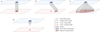 |
Fig. 1. Schematic illustration of several potential biases involved in the inference problem. Applied to the abundance determination problem, the observable space represents (notably) the oscillation frequency sets, while the unobservable space would represent the model abundances. Case a shows an ideal scenario, where for given constraints (blue circle) our modelling (in grey) provides unbiased abundances (red circle). Panel b: possible expression of physical processes that are missing or are poorly taken into account in the model. It thus results in physical biases although it has ideal observables. Case c provides an example of degeneracy, that is, parameters that can vary widely because they are too weakly constrained by the observables. The last panel d is a typical illustration of the solar problem, where no mixture seems to satisfy the constraints. In this case, inconsistencies in the model physics or much weaker constraints than actually provided by the oscillation frequencies must be considered in order to provide a solution. |
In this respect, the determination of abundances using realistic stellar models constitutes a textbook case that is potentially susceptible to a wide range of biases. Identified sources of difficulties undoubtedly reside in the complexity of the physics that must be considered. In particular, the equation of state, opacities (Kosovichev et al. 1992), or transport processes such as diffusion, turbulent mixing (Christensen-Dalsgaard et al. 1993), or radiative acceleration (Deal et al. 2018) can be evoked, whose consideration or exclusion may result in physical biases. Recent studies using model grids also suggest a strong anti-correlation between the mass and initial helium abundance estimates (Lebreton & Goupil 2014; Noll et al. 2021). This degeneracy makes the inference more complex by resulting in a high volatility of both parameter estimates. Moreover, when a large number of frequencies are available, as for the Sun, inversion techniques highlight significant discrepancies, and solar models are forced to choose between inconsistent abundances, densities, or convective zone (CZ) depths (Basu & Antia 2004; Asplund et al. 2009; Serenelli et al. 2009). In addition to these processes that directly involve the composition, additional uncertainties surrounding the near-surface region are to be faced, namely surface effects (Christensen-Dalsgaard et al. 1988). As a result of theoretical developments (Canuto 1997; Belkacem et al. 2021) and 3D hydrodynamical simulations (Belkacem et al. 2019; Schou & Birch 2020), our understanding of the mechanisms involved in these effects (as well as their contributions) has definitely improved. However, the more costly procedures (Mosumgaard et al. 2020) are generally avoided in favour of ad hoc corrections of the oscillation frequencies (Kjeldsen et al. 2008; Ball & Gizon 2014; Sonoi et al. 2015), which may affect stellar parameter estimates (Nsamba et al. 2018).
Methods allowing independent measurements of abundances (in particular helium) are therefore the subject of much investigation. The challenge is in fact twofold because a reliable estimate of abundances in turn would provide a constraint on the internal physics that depends on it.
The specific connection between composition and seismic properties of a star has long been known and can easily be understood through the structural change caused by ionisation if ever the abundances were to vary. The fact that this change is localised (in this case in the near-surface region) causes what is called a seismic glitch and manifests itself through an oscillatory deviation of the observed frequencies from a chosen reference (Gough 1990). Although this effect is not specific to the ionisation regions, these regions have benefited from numerous treatments, being both the most pronounced glitch and a potential marker of the helium abundance (Perez Hernandez & Christensen-Dalsgaard 1994; Lopes et al. 1997). From this point on, many studies (Monteiro et al. 1994; Basu et al. 1994; Monteiro & Thompson 1998, 2005; Gough 2002; Houdek & Gough 2007) considered various shapes of structural perturbations to analytically derive the expected frequency shifts. Most procedures exploit inversion formulae (Dziembowski et al. 1990; Gough & Thompson 1991; Antia & Basu 1994) and rely on an analytical modelling of the glitch to give a parameterised form of the oscillation. The expression thus obtained only needs to be fitted to data in order to provide information on the introduced parameters. In order to overcome dependences on irrelevant disturbances in the frequencies (e.g., surface effects in our case), it has also been proposed that the second differences, d2ν, be studied, rather than the frequencies directly (Gough 1990),
 (1)
(1)
where n and ℓ are the associated oscillation radial order and degree, respectively. The seismic diagnostic defined in this way is less sensitive to surface effects and core perturbations while highlighting signal that would come from an intermediate acoustic depth (Ballot et al. 2004).
The main benefit of this (now usual) approach is to avoid complex modelling and therefore part of the issues mentioned above. Being based on a model with far fewer parameters, which reflects a local rather than global structure, the method seeks to make the best use of the information residing only in the low-degree frequencies. Additionally, this procedure is lighter than a direct minimisation or inversion of the frequency differences, which makes it convenient for application to large samples of stars (Verma et al. 2019). On the other hand, it would be a mistake to think that the procedure is “model independent” as it depends on the form of the perturbation that is considered. This procedure may therefore well lead to nonphysical or inaccurate frequency shifts if it relies on a nonphysical or inaccurate glitch modelling. Moreover, if the parameter to be estimated does not appear directly in the model, there is no alternative to calibration on stellar models (Houdek & Gough 2007, 2011; Verma et al. 2014a, 2019), which adds its own uncertainty on the internal physics. This method is therefore largely dependent on the work done beforehand, and this first paper in the series is intended to cover this perspective. A second paper will focus on the seismic effects of the structural perturbation and on the information these effects provide about the abundances.
In the present paper, we propose a physical model of the ionisation region that allows us to derive a semi-analytic description of the structural perturbation caused by a change in abundances. In this respect, we first briefly describe previous modelling in Sect. 2 and provide more detailed picture of the most commonly used model of the ionisation glitch, which is that of Houdek & Gough (2007), hereafter HG07. The formalism of our own model of the ionisation region is introduced in Sect. 3 and its structural behaviour is studied in Sect. 4. In Sect. 5 we propose an analysis of the structural perturbation induced by the model and determine how it is related to analytical models of the ionisation glitch. The last part of the article is dedicated to our conclusions.
2. Previous seismic glitch frameworks
As we briefly mentioned, a twofold approach in the modelling is required to study seismic glitches. First, an expression for the structural perturbation must be considered, and then the shape of the associated frequency shift must be inferred.
2.1. Structural perturbation modelling
The modelling of the perturbation usually boils down to choosing a localised and parametrisable shape for the induced structural perturbation. Depending on the region and the phenomenon under study, various forms can be considered. For the transition between radiative and convective regions, very sharp shapes such as a Dirac or a step function are generally used to reflect a discontinuity in the density derivatives (Monteiro et al. 1994; Houdek & Gough 2007). However, because the ionisation region is more spread out, the shapes that are used to model the structural perturbations usually involve an additional dispersion parameter (Monteiro & Thompson 2005; Houdek & Gough 2007). In Fig. 2 we represent shapes introduced in previous papers with their associated parameterisation. In what follows, we focus on the most commonly used model (i.e. the one presented in HG07) for estimating helium abundances and on the derived expressions for the frequencies.
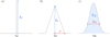 |
Fig. 2. Various shapes along with their associated parameters that are used to describe a structural perturbation. (a) Dirac function used in Monteiro et al. (1994) to model the variations in the acoustic potential (in the case of an overshoot) passing from a convective to a radiative region. For this modelling, it is only necessary to specify the acoustic depth τd and amplitude Aδ of the perturbation. (b) Triangular shape of the Γ1 perturbation in the second helium ionisation region as used in Monteiro & Thompson (2005). An additional parameter controls the width (β) of the perturbation. (c) Gaussian shape of the Γ1 perturbation in the second helium ionisation region as used in Houdek & Gough (2007). |

In HG07, the structural change caused by a change in helium abundance is first modelled as a Gaussian perturbation of the first adiabatic exponent Γ1 = (∂lnP/∂lnρ)S,
 (2)
(2)
The idea is as follows: The transition from a pure-hydrogen model to one partially composed of helium causes the appearance of a well in the Γ1 profile (cf. Fig 3). This results from the second helium ionisation to which the index HeII refers. While various analytical functions can be used to model a well, the well appears to be closely reproduced by a Gaussian expressed as a function of the acoustic depth  ; c(r), designating the sound speed at a given position. An important point is that if the depth, position, or width of the well depends on the helium abundance Y or on the thermodynamic conditions of the CZ, then a connection (though implicit) can be made between physical properties of the CZ and the parameters ΓHeII, ΔHeII, and τHeII.
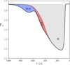 |
Fig. 3. Representation of a typical Γ1 profile in the ionisation region as a function of the acoustic depth τ (the surface corresponds to τ = 0). The helium abundance in this plot is Y ∼ 0.25. The contributions of the three main ionisation zones have been distinguished, i.e., the hydrogen (H), the first (HeI), and second (HeII) helium ionisation zones. Each of them causes a deviation from the Γ1 reference value of 5/3. |
Before further discussion, it may be useful here to clarify an ambiguity concerning the notation δ that symbolises the perturbation. Because it denotes a difference between two profiles (e.g., between profiles  and
and  ), the variable over which they are expressed has to be chosen carefully. For instance, for arbitrary variables x and y,
 (3)
(3)
As shown above, the notation δx allows us to overcome this ambiguity. This notation was introduced by Christensen-Dalsgaard & Thompson (1997), which developed this point extensively. Because the quantity x should vary in the same range for the two profiles A and B, it is natural to choose it as a normalised variable, for example, r/R, m/M, t = τ/τ0, ...(R, M, and  are the total radius, mass, and acoustic radius of the model). Moreover, the variable on which the perturbation is expressed can differ from the variable that was used to calculate the difference; both δxΓ1(x) and δxΓ1(y) have a meaning.
This point clarified, it appears that the perturbation used in HG07 for Eq. (2) is δτΓ1 because the Gaussian shape has been established after an expansion at fixed τ (cf. Eq (31) of HG07). As mentioned, δτ is ambiguous, however, if  . It can be replaced by δt following
 (4)
(4)
with  simply being the perturbation of a constant.
2.2. Expected frequency shift
The resulting signature in the frequencies can be divided in two distinct parts: the ionisation component, and the smooth component. We describe them in turn below.
Ionisation component. The connection between Eq. (2) and the frequency shift  is made by considering the following asymptotic form (Gough 1990):
![Mathematical equation: $$ \begin{aligned} \frac{\delta \nu _{n,\ell }}{\nu _{n,\ell }} = \int _0^1 \left[\mathcal{K} _{\rho c^{2}}^{~n,\ell } \frac{\delta _x \rho }{\rho }+ \mathcal{K} _{c^{2} \rho }^{~n,\ell } \frac{\delta _x c^{2}}{c^{2}}\right] \mathrm{d} x \sim \int _0^1 \mathcal{K} _{c^{2} \rho }^{~n,\ell } \frac{\delta _x \Gamma _1}{\Gamma _1} \mathrm{d} x ,\end{aligned} $$](/articles/aa/full_html/2021/11/aa41711-21/aa41711-21-eq13.gif) (5)
(5)
where  and
and  denote the usual structural kernels that can be found in Gough & Thompson (1991). This derivation, as well as the majority of the frequency shift treatment, will be fully discussed in a second paper. We emphasise that the perturbation used in Eq. (5) must be applied with caution. It can be shown that
![Mathematical equation: $$ \begin{aligned} \frac{\delta _x \Gamma _1}{\Gamma _1} = \frac{\delta _t \Gamma _1}{\Gamma _1} - \left[\frac{\delta \tau _0}{\tau _0}-\frac{\delta R}{R}+\frac{1}{x}\int _{0}^{x} \frac{\delta _{t} c}{c} \mathrm{d} x^{\prime }\right]\frac{\mathrm{d}\ln \Gamma _1}{\mathrm{d}\ln r} .\end{aligned} $$](/articles/aa/full_html/2021/11/aa41711-21/aa41711-21-eq16.gif) (6)
(6)
This nuance cannot be appreciated without the notation introduced here, however.
The frequency shift derived in HG07 is written as a continuous function of frequency,
 (7)
(7)
as are the second differences,
![Mathematical equation: $$ \begin{aligned} d^2\nu _{_{\Gamma _1}} = F_{_{\rm HeII}}A_{_{\rm HeII}}\nu e ^{-8\pi ^2 \Delta _{_{\rm HeII}}^{2} \nu ^{2}} \cos \left[2\left(2\pi \tau _{_{\rm HeII}} \nu +\epsilon _{_{\rm HeII}}\right)-\delta _{_{\rm HeII}}\right] ,\end{aligned} $$](/articles/aa/full_html/2021/11/aa41711-21/aa41711-21-eq18.gif) (8)
(8)
with AHeII = πΓHeII/τ0. FHeII and δHeII are functions of the other parameters and the frequency (although it is assumed that they only fluctuate slowly with it). The total number of parameters is therefore only four.
Smooth component. The helium component is not the only perturbation expected in the second differences. In addition to the signature of the transition between radiative and convective regions, a smooth component d2νs can also be considered and modelled as
 (9)
(9)
The idea is to first consider a star that would not contain any glitch. Without any structural perturbation (thus simplifying the problem), it can be assumed that its frequencies follow the asymptotic expansion provided by Tassoul (1980), that is,
![Mathematical equation: $$ \begin{aligned} \nu _{n,\ell } = \left[\frac{1}{2}(2n+\ell +\varepsilon )+\frac{2V_\ell }{2n+\ell +\varepsilon }\right]\Delta \nu + \mathcal{O} \left(\frac{1}{{\nu _{n,\ell }}^2}\right) ,\end{aligned} $$](/articles/aa/full_html/2021/11/aa41711-21/aa41711-21-eq20.gif) (10)
(10)
where ε and Vℓ are two dimensionless parameters that are independent of the radial order n, and Δν ≡ 1/2τ0 is the asymptotic large frequency separation. The last term of Eq. (9), which is proportional to ν−3, can then be interpreted as the leading term of the second differences applied to Eq. (10),
 (11)
(11)
However, it is difficult to give as convincing a justification for the other terms, which hide a much more complex deviation to the asymptotic expansion. Houdek & Gough (2011) in particular listed hydrogen ionisation, a sharp stratification of the upper layers of the convection zone, non-adiabatic processes, and turbulent perturbations caused by the oscillations. In the end, this component adds four free parameters to those identified so far. It should be noted that the combination of positive powers of ν introduced in Verma et al. (2014a) to describe the smooth component is incompatible with the asymptotic expansion (10).
2.3. Improvements and limits of the approach
Although it is not apparent from this short summary, the derivation of Eqs. (5)–(8) is as complex as it is intricate, and an analytical derivation of second differences therefore requires making use of many approximations. The first consequence is that a fit of the second differences with Eq. (8) only allows a very approximate retrieval of the parameters introduced in Eq. (2). HG07 revealed typical discrepancies of 50, 33, and 25% on parameters ΓHeII, ΔHeII, and τHeII, respectively. These differences can be reduced to 5, 15, and 15% by introducing a frequency dependence in ϵHeII that is induced by the cut-off frequency and a more complete model by adding the first helium ionisation contribution in Eq. (2) (see Fig. 3). Having now two Gaussians (indexed by HeI and HeII), the expected second differences become
![Mathematical equation: $$ \begin{aligned} d^2\nu _{_{\Gamma _1}} = \sum _{i~ =~\{\mathrm{HeI},\,\mathrm{HeII}\}} F_iA_i\nu e ^{-8\pi ^2 \Delta _i^{2} \nu ^{2}} \cos \left[2\left(2\pi \tau _i \nu +\epsilon _i(\nu )\right)-\delta _i\right] \end{aligned} $$](/articles/aa/full_html/2021/11/aa41711-21/aa41711-21-eq22.gif) (12)
(12)
instead of Eq. (8). Because the parameters of the two Gaussians are not independent, three of them are fixed in HG07 by the empirical relations AHeI/AHeII = 0.5, ΔHeI/ΔHeII = 0.9, and τHeI/τHeII = 0.7. The number of independent parameters in the expression is still four (only one is needed to determine ϵHeI(ν) and ϵHeII(ν)). However, despite the substantial improvement in the parameter retrieval, Eq. (8) remains the currently most frequently used equation for studying ionisation glitches (Verma et al. 2017, 2019; Farnir et al. 2019).
More importantly, the abundances, and in particular, the helium abundance Y, do not appear directly as parameters in Eq. (12). As mentioned above, without further theoretical work to establish a dependence between these parameters and Y, calibration based on realistic models therefore seems to be necessary in order to make it appear. This is probably the greatest criticism that can be made of the method. To illustrate this point, we place ourselves in a broader framework and consider two models 𝒫 and ℳ⋆ that represent the structural perturbation caused by a change in helium δY and the structure of a realistic stellar model, respectively. The first is parameterised by a set of values ⃗θp and the second by the set ⃗θ⋆ from which we explicitly distinguish Y for its particular role in this context. As an example, if the model 𝒫 is chosen to be a Gaussian, as done by HG07 (Eq. (2)), it would then involve three parameters ⃗θp = (ΓHeII,ΔHeII,τHeII). In contrast, ⃗θ⋆ instead contains quantities needed to calculate a realistic model, such as fundamental parameters (mass M⋆, radius R⋆, age A⋆, etc.), but also all the quantities required to model the physical processes involved in the star (overshoot, mixing length, parameters implied in diffusion or rotation, etc.; cf. Lebreton & Goupil 2014, which provides a broad idea of the various possible prescriptions). As a result, ⃗θ⋆ generally contains many more components than ⃗θp. With this in mind, we would like to be able to relate a fitted set of parameters, ⃗θp, to a difference in helium δY from a chosen reference Y. For this purpose, the solution proposed by calibration is to assimilate the perturbation model 𝒫 to a model perturbation δℳ, and therefore to assume
 (13)
(13)
in order to numerically derive a relation ⃗θp(δY). We note that Eq. (13) is equivalent to Eq. (33) of HG07 when 𝒫 is chosen to be the sum of two Gaussians and Y = 0 as a reference (although the choice of ⃗θ⋆ is not specified in HG07). In order to be able to associate a set of parameters ⃗θp with a unique δY, the calibration method therefore makes the assumption that ∂ℳ⋆/∂Y does not depend on the reference point (Y; ⃗θ⋆). However, despite some arguments that are given in favour of a relative independence regarding the choice of Y, we show in Sect. 5 that this assumption about ⃗θ⋆ is inadequate. These dependences cannot be reflected in model 𝒫, which depends on too few parameters, namely ⃗θp (we note that this is part of the reasons for introducing 𝒫 in the first place). To minimise the error that is introduced, it is then necessary to determine as many ⃗θp(δY) relations as stars that are studied (given independent constraints on ⃗θ⋆, see Verma et al. 2019), which can be quite costly. Moreover, by using such a relation anyway, we reintroduce the biases we wished to avoid when studying the ionisation glitch. The relation that is obtained will largely depend on the physics considered in ℳ⋆, in particular, on mechanisms that are not necessarily relevant for modelling the ionisation region.
To summarise, even though it is based on a more sophisticated model than previous methods, the method described above faces challenges that are mainly due to its empirical introduction. In particular, the lack of an explicit dependence on Y greatly reduces its applicability. We would like to reverse the approach. The idea is firstly, to introduce a physics-based parameterisation allowing inferences concerning ionisation regions, and secondly, to give a mathematical description regarding the Γ1 profile. The challenge is to provide such a modelling while keeping the number of parameters as low as possible. This problem is addressed in the two following sections.
3. First adiabatic exponent in an ionisation region
In order to model the structure of the ionisation zone, we first try to provide an analytical expression of Γ1 in this specific region. As previously mentioned, we avoid introducing it through similarities with mathematical functions, but rather derive it from thermodynamic relations. Expressions like this have already been obtained (e.g. Cox & Giuli 1968; Kippenhahn et al. 2012), but are generally functions of the occupation number rather than state variables (such as T and V). Furthermore, because the chemical equilibrium resulting from Saha’s equations is complex, these equations are generally solved numerically, and analytical expressions are limited to the ionisation of single species. We try to present in the following the simplest model that can nevertheless explicitly involve chemical composition.
3.1. Free energy
Our starting point is the free energy of a multi-component ideal gas, that is,
 (14)
(14)
where V designates the volume, kT is the temperature expressed in energy units, and Nα and μα(T, V, Nα) are the number and chemical potential of particles of type α. In the context of partial ionisation, α refers to (i, r), 1 ≤ i ≤ Nsp being an index on the chemical species and 0 ≤ r ≤ zi the ionisation state (where zi is the atomic number), or it may also correspond to e for an electron. The key point of Eq. (14) lies in its ability to provide us with the pressure P and entropy S through its first derivative. Moreover, its second derivative gives access to virtually any other thermodynamic quantity ranging from the speed of sound through the adiabatic exponents including Γ1 to various compressibilities. Before the calculations, we would like to define the particular meaning of a derivative in stellar physics compared with pure thermodynamics in more detail. The first adiabatic exponent is often defined as follows:
 (15)
(15)
where the subscript S denotes a partial derivative taken at constant entropy. The above expression can easily be rewritten using the more common variables T and V,
![Mathematical equation: $$ \begin{aligned} \begin{aligned} \Gamma _1= \frac{V}{P} {\left(\frac{\partial S}{\partial T}\right)_{V}}^{-1}\left[\left(\frac{\partial P}{\partial T}\right)_{V}\left(\frac{\partial S}{\partial V}\right)_{T}-\left(\frac{\partial P}{\partial V}\right)_{T}\left(\frac{\partial S}{\partial T}\right)_{V}\right] \end{aligned} .\end{aligned} $$](/articles/aa/full_html/2021/11/aa41711-21/aa41711-21-eq26.gif) (16)
(16)
Although this equation is generally valid, its use in the present case requires some clarification because it only mentions the two state variables T and V and does not explicitly show the dependence on the various number of particles Nα. Assuming that species are indexed so that zi = i ( potentially being null), the free energy introduced in Eq. (14) is a function of Nsp(Nsp + 3)/2 + 3 variables. As a result, the partial derivatives of Eqs. (15) and (16) are generally ambiguous unless some indication is given concerning the Nsp(Nsp + 3)/2 + 1 implicit conservation equations. Partial derivatives are commonly considered at constant values of state variables, for example,
 (17)
(17)
However, it is clear that the derivatives appearing in Eq. (16) (and second derivatives of F considering Eq. (17)) are not of this kind. As mentioned in the introductory section, the Γ1 profile used in stellar physics shows clear signs of ionisation that derivatives taken at constant Nα do not. This choice imposes a particular ionisation state in the whole region (described by the constant Nα values), which instead should fluctuate widely with the thermodynamic conditions in the CZ. The solution is to consider the following conservation equations instead:
![Mathematical equation: $$ \begin{aligned}&\forall i,~\forall r>0, \quad \mu _i^r+\mu _e-\mu _i^{r-1} = 0 \qquad \quad \left[~\frac{N_{\rm sp}(N_{\rm sp}+1)}{2}~\right] \end{aligned} $$](/articles/aa/full_html/2021/11/aa41711-21/aa41711-21-eq29.gif) (18)
(18)
![Mathematical equation: $$ \begin{aligned}&\forall i, \quad \sum _{r=0}^{z_i} N_i^r = N_i = \mathrm{cnst} \qquad \qquad \quad \qquad ~~~ \left[~N_{\rm sp}~\right]\end{aligned} $$](/articles/aa/full_html/2021/11/aa41711-21/aa41711-21-eq30.gif) (19)
(19)
![Mathematical equation: $$ \begin{aligned}&\sum _{i=1}^{N_{\rm sp}}\sum _{r=1}^{z_i} rN_i^r = N_e \qquad \qquad \qquad \qquad \qquad \quad \left[~1~\right]. \end{aligned} $$](/articles/aa/full_html/2021/11/aa41711-21/aa41711-21-eq31.gif) (20)
(20)
The first equation corresponds to the chemical equilibrium of the ionisation reaction,  . The second equation is merely the conservation of each atom number and can also be considered as a chemical equilibrium in the absence of reactions and homogeneous mixing of the CZ. The last expression corresponds to the overall charge equilibrium, that is, electroneutrality. This set of relations can be interpreted as a local equilibrium for given temperature and volume conditions that should be verified at each point of the CZ, and partial derivatives taken with respect to these constraints are hereafter be denoted with the subscript EQ. The resulting number of constraints is indicated in square brackets, and these constraints add up to Nsp(Nsp + 3)/2 + 1 as required.
Hereafter, we use the notation  to designate a second derivative taken with respect to β (subject to Nα being constant) and then α (subject to EQ). For example, Eq. (16) becomes
 (21)
(21)
by using relations (17). Considering Eq. (14), the evaluation of the Eq. (21) now requires finding  at a given EQ.
3.2. Approximate local equilibrium
To solve the system (18)–(20), the expression of the chemical potential of each particle must first be explicitly be written out. We have
 (22)
(22)
with λα(T) and 𝒵α(T) the thermal De Broglie wavelength and the canonical partition function of a particle α, respectively. Conditions (18) thus become
 (23)
(23)
with  the occupation number of state (i,r). In our effort to obtain the simplest model that can be used to handle chemical composition, the ideal gas assumption remains relevant. We note, however, that in order to take the ionisation process in a more accurate way into account, it would be necessary to consider the Coulomb effects (Rogers 1981; Rogers et al. 1996). In this ideal case,
  and 𝒵e are often approximated by (e.g., Kippenhahn et al. 2012)
 (24)
(24)
 (25)
(25)
with  describing the fine structure of state (i,r) approached by the degeneracy of the ground state
  , and
, and  the ionisation energy separating state (i,r) from (i,r − 1) (
 is then the energy from the reference state (i,0), which is assumed here to have a null internal energy). The second approximation (25) directly results from neglecting the electron spin energy contribution.
Thus, conditions (23) simply become Saha’s equations,
 (26)
(26)
These equations are highly coupled, especially because of the term Ne, which can be expressed from (20) as
 (27)
(27)
with N = ∑iNi and xi = Ni/N the total number of atoms and the number abundance of element i, respectively, which are two constants from (19). Because of this, Saha’s equations are generally solved numerically by iterating over estimates of the  . In the following, we try to give analytical approximations by considering a few simplifying assumptions. First, we introduce the cumulative occupation number
  , which is more suited to the study of Eqs. (26) (Baker & Kippenhahn 1962). We also use from this point the convention

In this way, we can write  with
with
 (28)
(28)
the mean number of electrons per atom. Saha’s equations can be rewritten as
 (29)
(29)
with the convention  (and by definition
  ). We start by noting that it is rare to find more than two ionisation states simultaneously for a given element. It is thus advantageous to make the following approximation (Baker & Kippenhahn 1962):
 (30)
(30)
Then, in the single domain of interest ( ), (29) is approached by
 (31)
(31)
A final assumption is needed to express  as a function of
  only and to completely decouple the system. One idea may be to exploit the fact that stars are predominantly composed of hydrogen in number: For typical Y values (i.e. 1/4 < Y < 1/3), x1 ∼ 0.89 − 0.92, and it can be seen using (28) that after a complete ionisation of the hydrogen,
  . Another bound can then be obtained on
  because the latter tends asymptotically towards ∑izixi = 2 − x1 + ∑i > 2(zi − 2)xi. Because for heavy elements (i > 2), mi ≃ 2zimu with mi the mass of atom i and mu the atomic mass unit, and because the mean mass m0 < 2mu in a stellar mixture, we have m0/mi < 1/zi. Finally, the number and mass abundances are related by xi = m0Xi/mi, meaning that
  should remain below the upper boundary 2 − x1 + Z ∼ 1.1 with Z = ∑i > 2Xi the metal abundance in mass. This simple reasoning allows us to convince ourselves that
  must remain close to 1 when the ionisation of hydrogen is completed, and in a way relatively independent of the mixture under consideration.
The pragmatic assumption can therefore be made that the ionisation of hydrogen occurs first and is completed before any other ionisation begins. Thus we can use the fact that hydrogen is the dominant component to approximate  by the mean electron number in a pure-hydrogen model. Although this is not entirely true (particularly not for a low ionisation state), this assumption greatly simplifies the problem. For all elements i > 1,
  , which, as discussed above, is a reasonable approximation. For the ionisation equation corresponding to hydrogen (i = 1), we instead approximate
  . Our version of Saha’s equations can thus finally be written as
 (32)
(32)
with n = 2 if i = 1 and n = 1 in any other case. We define  as the term on the right-hand side (RHS) of (32). We then obtain the desired relations.
![Mathematical equation: $$ \begin{aligned} { y}_1^1(T,V)&= \frac{1}{2}\left[\sqrt{K_1^1(K_1^1+4)}-K_1^1\right]\end{aligned} $$](/articles/aa/full_html/2021/11/aa41711-21/aa41711-21-eq70.gif) (33)
(33)
 (34)
(34)
It is easy to retrieve  from there using
  (as well as
  using
using  ). Figure 4 shows a comparison of hydrogen and helium ionisation fractions
  , and
, and  obtained analytically from (33) and (34) for given T and V values with the numerical solution of Saha’s Eqs. (26). The result is shown as a function of the normalised acoustic depth t so that it can be reduced to a comparison of profiles rather than a (V, T) mapping. The solution presented above appears to be satisfying considering the number of assumptions made. However,
  is slightly underestimated because
  is slightly lower than 1 in the first helium ionisation region. The opposite reasoning holds for the second helium ionisation region.
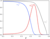 |
Fig. 4. Comparison of approximations (33) and (34) in the case i = 1, 2 (opaque curves) with the numerical solution of (26) (dashed light curves) for solar near-surface conditions of (T, V, Xi > 1). These quantities are represented as a function of the normalised acoustic depth t = τ/τ0 (the surface is then located at t = 0), along which all future plots are represented. |
3.3. First adiabatic exponent
Approximations (33) and (34) allows us to derive all derivatives appearing in (21). First of all, we have
 (35)
(35)
where we explicitly made the  apparent to fully exploit relations (33) and (34). It is straightforward to show that we simply retrieve the classical expression for the pressure in an ideal gas. Second derivatives taken at EQ ensue,
![Mathematical equation: $$ \begin{aligned} \partial _{VV}^2 F&= \frac{NkT}{V^2}\left[1+\sum _{ir}x_i{ y}_i^r\left(1-\frac{\partial \ln { y}_i^r}{\partial \ln V}\right)\right]\end{aligned} $$](/articles/aa/full_html/2021/11/aa41711-21/aa41711-21-eq82.gif) (36)
(36)
![Mathematical equation: $$ \begin{aligned} \partial _{TV}^2 F&= \frac{-Nk}{V}\left[1+\sum _{ir}x_i{ y}_i^r\left(1+\frac{\partial \ln { y}_i^r}{\partial \ln T}\right)\right]. \end{aligned} $$](/articles/aa/full_html/2021/11/aa41711-21/aa41711-21-eq83.gif) (37)
(37)
More explicit expressions can be deduced by writing  and exploiting Eq. (32),
 (38)
(38)
 (39)
(39)
 (40)
(40)
 standing for Kronecker’s symbol. Resulting expressions of the derivatives are
![Mathematical equation: $$ \begin{aligned} \partial _{VV}^2 F&= \frac{NkT}{V^2}\left[1+\sum _{ir}x_i{ y}_i^r\left(1-\frac{1-{ y}_i^r}{1+\delta _i^1(1-{ y}_i^r)}\right)\right]\end{aligned} $$](/articles/aa/full_html/2021/11/aa41711-21/aa41711-21-eq89.gif) (41)
(41)
![Mathematical equation: $$ \begin{aligned} \partial _{TV}^2 F&= \frac{-Nk}{V}\left[1+\sum _{ir}x_i{ y}_i^r\left(1+\frac{(1-{ y}_i^r)\phi _i^r}{1+\delta _i^1(1-{ y}_i^r)}\right)\right]. \end{aligned} $$](/articles/aa/full_html/2021/11/aa41711-21/aa41711-21-eq90.gif) (42)
(42)
The calculation of the two remaining derivatives is more subtle, however. We propose here to start with a determination of the energy E,
 (43)
(43)
Because  and
and  , it might be tempting to take directly the derivatives of (43) using dE = TdS − PdV. However, in the present framework,
 (44)
(44)
Clearly, the last two sums cancel each other because  , which is verified in our derivation as long as we define
  . Electroneutrality, used in line 2 of Eq. (44), is also verified by imposing
  . According to Eq. (18),
  , and the third term must also cancel exactly. In practice, Eq. (18) is too complex to be perfectly solved, and numerical calculations as well as analytical approximations can lead to some small departures from exact cancellation. These may lead to slight thermodynamic inconsistencies (which could be corrected through departures from equality of partial mixed second derivatives of state functions such as the free energy F). However, these residuals remain small, and we considered that chemical equilibrium is perfectly satisfied. The only part that therefore remains from (44) is the following well-known identity:
 (45)
(45)
This means that  and
and  . It follows from Eq. (43) that
![Mathematical equation: $$ \begin{aligned} \partial _{VT}^2 F&= \frac{-Nk}{V}\left[1+\sum _{ir}x_i{ y}_i^r\left(1+\frac{(1-{ y}_i^r)\phi _i^r}{1+\delta _i^1(1-{ y}_i^r)}\right)\right]\end{aligned} $$](/articles/aa/full_html/2021/11/aa41711-21/aa41711-21-eq102.gif) (46)
(46)
![Mathematical equation: $$ \begin{aligned} \partial _{TT}^2 F&= \frac{-Nk}{T}\left[\frac{3}{2}+\sum _{ir}x_i{ y}_i^r\left(\frac{3}{2}+\frac{(1-{ y}_i^r){(\phi _i^r)}^{2}}{1+\delta _i^1(1-{ y}_i^r)}\right)\right]. \end{aligned} $$](/articles/aa/full_html/2021/11/aa41711-21/aa41711-21-eq103.gif) (47)
(47)
Denoting the bracket part of  as
as  , we obtain
 (48)
(48)
where
 (49)
(49)
 (50)
(50)
 (51)
(51)
 (52)
(52)
The various symmetries present in these equations may give the impression that expression (48) can be further simplified. We show in Appendix A that Γ1 can finally be written as
 (53)
(53)
with 0 ≤ γ1 < 1 simply expressed as
 (54)
(54)
Together with Eqs. (32)–(34), Eqs. (52)–(54) provide an analytical approximation of Γ1(T, V, xi) in the CZ. Even though this expression is applicable to any kind of mixture (but is assumed to be homogeneous in the CZ!), the following examples are based on a hydrogen-helium mixture of mass fraction 1 − Y and Y (Y = 4x2/(1 + 3x2)) to facilitate the study. We recall that N/V = ρ/m0, and represent the resulting Γ1(ρ, T, Y) in Fig. 5 for Y = 0.25 as well as for extreme values, Y = 0 and Y = 1. Each panel also shows the relation ρ(T) extracted from a CESTAM solar model (Morel & Lebreton 2008; Marques et al. 2013). The latter is obviously only indicative as it depends on the composition, but it still provides an idea of what part of the map is visible in a Γ1 profile. The figure clearly reflects the Γ1 depressions caused by (from left to right) the hydrogen and first and second helium ionisations. Each element contribution is enhanced in the left panels. In the top right panel, the superposition of the hydrogen and helium first ionisation zones in typical solar conditions is presented, whereas the distinction becomes apparent at lower densities. In contrast, this signature appears to be more diffuse at the highest densities. This behaviour appears in each panel and is further discussed in Sect. 4. The last frame shows the variation δρ, TΓ1 caused by a change in helium abundance, δY = 0.1, from a reference value Y = 0.25. Although the variables are not normalised, the notation δρ, T is still meaningful because Γ1 does not refer to a profile here, but to a function defined for all (ρ, T) at a given Y. As expected, this variation in abundance causes the two helium wells to become lower while elevating the hydrogen well. However, the variations appear to be fairly disproportionate between the two elements. The change in the hydrogen ionisation region would be barely noticeable considering the typical solar relation ρ(T), shown in black. Appendix A provides clues that help to understand this difference in behaviour as well as the particular shape of the perturbation in the hydrogen region compared with that of helium. In particular, the amplitude of the variation seems more related to the relative change δxi/xi than δY. While we have δx1 = −δx2 for the hydrogen-helium case, we see that δx1/x1 = −δx2/x1 = −(x2/x1)δx2/x2 with (x2/x1) = 1/12 for Y = 0.25. This explains why the change in hydrogen is expected to cause a variation that is an order of magnitude lower than the change in helium.
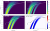 |
Fig. 5. 2D maps of the first adiabatic exponent obtained from Eq. (53). Panels a–c: Γ1(ρ, T, Y) as a function of ρ and T for different values of Y. Panel d: variation δρ, TΓ1 caused by a perturbation δY = 0.1 from a reference value Y = 0.25. The dashed line in each panel shows the relation ρ(T) extracted from a CESTAM solar model. |
Although Eqs. (53) and (54) appear to be promising, they are merely functional forms and do not allow us at this point to model a parameterised structure of the ionisation region. However, Γ1, ρ and T are closely related in stellar interiors.
4. Model structure and properties
In this section we obtain the stellar structure associated with the Γ1 expression derived in the previous section (see Eqs. (53) and (54)). To do this, we assume the conditions of a CZ that correspond to the assumptions for deriving the first adiabatic exponent. These are (1) an isentropic region, (2) chemical equilibrium at any position, (3) uniform abundances (due to homogeneous mixing), and (4) electroneutrality at any position. The last three conditions correspond to applying EQ conditions at any point in the region. Moreover, to avoid getting lost in the many possibilities offered by these relations in terms of the mixture, we again consider a relation of the form Γ1(ρ, T, Y) in this part. It is possible o generalise all the observations made here to any (reasonable) mixture by replacing Y by Xi > 1, however.
4.1. Ionisation region structure
As mentioned above, the quantities Γ1, ρ and T are not independent in stellar interiors, and although it may be interesting to study Γ1 for any condition of temperature and density, relevant profiles in these environments are much more constrained. The appropriate equations to express these constraints are the well-known hydrostatic equilibrium and Poisson’s equation assuming spherical symmetry,
 (55)
(55)
 (56)
(56)
where we have introduced the additional intermediate variable g, the norm of the gravity field. At this point, it is important to recall that we try to account for the variation of T and ρ in the region rather than that of P. This can be achieved by noting that for any quantity α,  . Then, crucially, we note that derivatives taken with respect to the radius r such as dlnP/dlnα = (dlnP/dr) (dlnα/dr)−1 exactly correspond to derivatives taken at constant entropy and EQ (cf. assumptions 1–4 at the beginning of the section). Using this for α = T, ρ, Eqs. (55) and (56) can be changed into a differential system of three equations, the solution of which is (T, ρ, g)
 (57)
(57)
 (58)
(58)
 (59)
(59)
where we introduced the second adiabatic exponent Γ2 such that  . Its expression can easily be deduced from Γ1 by noting that their definitions are symmetrical with respect to a change V ↔ T,
![Mathematical equation: $$ \begin{aligned} \begin{aligned} \frac{\Gamma _2}{\Gamma _2-1}&= \frac{T}{P} {\left(\frac{\partial S}{\partial V}\right)_{T}}^{-1}\left[\left(\frac{\partial P}{\partial T}\right)_{V}\left(\frac{\partial S}{\partial V}\right)_{T}-\left(\frac{\partial P}{\partial V}\right)_{T}\left(\frac{\partial S}{\partial T}\right)_{V}\right] \end{aligned} .\end{aligned} $$](/articles/aa/full_html/2021/11/aa41711-21/aa41711-21-eq120.gif) (60)
(60)
An analogous expression to Eq. (53) can be provided for Γ2,
 (61)
(61)
by introducing
 (62)
(62)
The pressure can also be removed using the ideal gas law (35), which leads to the following system:
 (63)
(63)
 (64)
(64)
 (65)
(65)
All quantities on the RHS are functions of ρ, T, and g only (for a given value of Y). By imposing the central values Tc and ρc (gc must be null in any case), we now have a complete system, the solution of which is  . The resulting model is fully convective and contains an ionisation region whose properties are controlled by the triplet (Y, Tc, ρc). Although this triplet seems the most intuitive, it is possible to parameterise the model by considering other triplets derived from these three quantities. Hereafter, we instead consider the following dimensionless parameterisation:
 (66)
(66)
![Mathematical equation: $$ \begin{aligned} \psi _{\rm CZ}~&\equiv ~ \ln \left[\frac{\rho _c h^3}{2m_u(2\pi m_e kT_c)^{3/2}}\right], \end{aligned} $$](/articles/aa/full_html/2021/11/aa41711-21/aa41711-21-eq128.gif) (67)
(67)
 (68)
(68)
where we introduced the Planck constant h, the electron mass me, and the ionisation potential of hydrogen χH. This particular choice and the associated notations will become clearer later on. At this point, this choice entirely constrains the Γ1 value at the centre, the latter being only a function of Y,  (we recall that
  ), and χH/kT (cf. Eqs. (32)–(34) and Eqs. (52)–(54)). However, their impact on our model is much more significant than this.
Physical interpretation of the parameters. Because Y(r) is constant (see assumption 3), the helium amount Ys is clearly imposed at any location of the model up to the surface symbolised by the index s.
The second parameter derives its notation from its close link to the electron degeneracy parameter  in the ideal gas limit. We can show that
 (69)
(69)
However, as long as Γ1 = 5/3 (i.e., outside the ionisation region), ρ ∝ T3/2, which means that ψ is preserved. Therefore ψCZ approximates the electron degeneracy parameter from the centre up to the ionisation region.
The last parameter ε results from the ratio of two energy scales in the model. The first is the ionisation energy for the hydrogen (13.6 eV), and the second is the order of magnitude of the thermal energy at the centre of the model (∼keV), making this ratio generally rather small (hence the notation ε). Through conservations, we just saw that Ys and ψCZ reflect properties of the ionisation region; this also holds for its helium abundance and electron degeneracy. It is complicated to apply this to ε because χH/kT varies by several orders of magnitude in the model. We try to give an intuitive understanding of its impact on the model structure, however. We first note that if Γ1 did not depend on χH/kT, the latter would be equal to 5/3 in the whole model. Because Γ1 would depend only on Y (which is constant) and  , the value of which is fixed as long as ρ ∝ T3/2, the first adiabatic exponent would keep its central value, that is, 5/3. The value of χH/kT at a given position then alone determines whether Γ1 deviates from the value 5/3, that is, if the ionisation region is entered starting from the model centre. It can be shown that the ionisation of the element i in state r takes place when
  . The role of ε can now be clearly identified: When ε is to be large (e.g., of the order of −ψ), the ionisation will be complete close to the centre. In contrast, if ε is small before −ψ, it will take until T ≪ Tc for the ionisation to be completed and the region will be shifted closer to the surface. This shows that although it is not explicitly linked to any quantity of the ionisation zone, ε controls the extent of the region.
After this physical interpretation for the parameters, we now try to provide a geometrical interpretation of the impact of each parameter regarding the Γ1 profile. We rely on Fig. 6, which shows the Γ1(t) (with t = τ/τ0, the normalised acoustic depth) profiles resulting from multiple parameter sets (Ys, ψCZ, ε) by varying them one by one around a reference value.
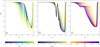 |
Fig. 6. Γ1(t) profiles obtained by considering various sets (Ys, ψCZ, ε) around a reference |

Geometrical interpretation of the parameters regarding the Γ1 profile. We gave a representation of Γ1(t) for all possible values of Ys in panel a of Fig. 6, including such extreme cases as pure-hydrogen or helium stars. As expected, the profile changes from one that only shows the hydrogen well (Ys = 0) to one that only shows the two helium wells (Ys = 1), passing through profiles that account for the three components (0 < Ys < 1). Clearly, increasing Ys has the effect of extending both helium wells while reducing the hydrogen well.
The effects of modifying ψCZ are shown in panel b of Fig. 6. The range under consideration corresponds to typical solar degeneracy values ranging from the surface (−12: very low degeneracy) to the centre (−2: high degeneracy). The impact is again clearly visible: A high degeneracy tends to spread out the ionisation wells, making them indistinguishable when ψCZ → −2. In the opposite situation, low degeneracies in the ionisation region result in much deeper and localised wells. It is even possible to distinguish the contributions of the hydrogen and the first helium ionisations when ψCZ approaches −12. This last point is consistent with what we showed in Fig. 5 : high degeneracies correspond to relations of the form lnρ(T) = C + (3/2)lnT with high C values. Thus, structures with high ψCZ correspond to ρ(T) that are located in the upper part of Fig. 5, where the ionisation regions tend to overlap. The opposite reasoning holds just as well.
The impact of ε is illustrated in panel c of Fig. 6. As expected from the previous paragraph, varying its value from 0.01 to 0.05 results in a shift of the ionisation region. However, this change differs between each well, the HeII well is more strongly affected than the hydrogen well. In order of magnitude, this effect can be explained by the dependence of the normalised acoustic depth on temperature close to the surface:  . Thus, for a given ionisation temperature Tion, the impact of ε becomes more noticeable on the associated depth tion as Tion is high. This reasoning also explains why the shift does not appear to be linear with respect to ε for a given well (this is particularly visible for the HeII well); this shift varies as
  .
.
Figure 6 shows an interesting point of the model defined with (Ys, ψCZ, ε): the relative independence of the impact of each parameter. When each well is treated as a distribution, all parameters appear to impact a specific moment. For instance, Ys appears to be directly related to the distribution area and does not impact the shapes of the wells or the position much (for reasonable values of Ys). ψCZ is clearly related to the dispersion of the distribution and ε to its position. These distinct impacts on the structure are encouraging for subsequent parameter retrieval as we can expect to avoid degeneracy biases.
4.2. Comparison with a realistic stellar model
The first and most important point to address is to verify the extent to which the model described in this article can approximate the ionisation region structure of a realistic stellar model. To do this, we compare in panel a of Fig. 7Γ1(t) profiles extracted from a CESTAM solar model and from our model for a particular parameter set  . These values were chosen so that
 (70)
(70)
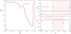 |
Fig. 7. Correspondence between the CESTAM profiles and their respective analogues in our model. (a) Comparison of |


is minimal. The behaviour of the realistic model can clearly be very well reproduced, the curves differ mainly in only two regions. A first difference is located in the first helium ionisation region (0.12 < t < 0.18), where the depth of the well is slightly overestimated. This is mainly caused by the assumption made in Sect. 3.2, where we assumed that  in the helium ionisation region and thus underestimated the number of electrons in the HeI region. This causes the ionisation to start slightly deeper in the model and therefore to be more localised. By reducing the dispersion of the HeI well, the assumption slightly enlarged its depth. As expected, another difference is visible in the atmospheric region (t < 0.03). Because the ionisation has not yet started, our Γ1 still has the value 5/3, which is obviously not the case in a realistic model containing an atmospheric modelling. The overall profile shape is nevertheless well reproduced in the ionisation region, especially considering that only three parameters need to be adjusted.
A second point to be clarified is the exact meaning of the adjusted values  regarding the realistic model. When the minimal differences (δtΓ1/Γ1)2 are assumed, the model parameterised by
  is interpreted as being the closest to the CESTAM model from the perspective of a particular structural aspect. This aspect will be discussed in much more detail in a forthcoming paper, but we can already relate it to the “visible” part of the structure through the frequency shift considering Eq. (5). In this sense, if our modelling and its interpretation are correct, we can expect our parameters to approach the quantities they refer to in the realistic model. However, in previous paragraphs we gave an understanding of these parameters in our model, but a realistic model only locally verifies the assumptions used to derive our structure. In particular, the relation between P and ρ is described by
  rather than Γ1, the two differing outside the isentropic region. Accordingly, we expect the adjusted values to approximate the CESTAM model quantities where assumptions 1 to 4 are verified, that is, in the CZ. For the helium abundance Ys, because Ys = Y(t) at any position of our model, the value
  should approximate YCESTAM(t) in the whole CZ up to the atmosphere. In the case of ψCZ, we saw that the approximation remains valid as long as Γ1 = 5/3, therefore we expect
  to approach ψCESTAM(t) in the CZ part that is located below the ionisation region. As mentioned, because ε does not relate to any particular quantity of the CZ, it is difficult to deduce more than the position of the ionisation region. These approximations can be summarised as follows:
 (71)
(71)
 (72)
(72)
with BCZ, ATM, and ION designating the base of the convective zone, the base of the atmosphere, and the end of the ionisation region, respectively. We illustrate this point in panels b and c of Fig. 7 by representing both YCESTAM(t) and ψCESTAM(t), as well as the estimates  and
and  obtained through the minimisation of Eq. (70). We also highlight the regions in which the quantities are expected to correspond to each other based on Eqs. (71) and (72). The values thus obtained
  = (0.255, −5, 0.015) are consistent with the CESTAM quantities in the associated regions (see panels b and c of Fig. 7 and Table 1).
Inferred electron degeneracy parameter and helium abundance and actual CESTAM quantities.
It is risky to be quantitative about this result because there are no obvious values with which the difference can be compared; in particular the relative difference does not appear to be relevant. Nevertheless, this example strongly suggests that the modelling defined here allows us to define structures that are close to realistic models (in the sense of criteria (70)) and to also obtain similar helium abundances and electron degeneracies in the regions of interest.
5. Analysis of first adiabatic exponent perturbations
So far, we focused on introducing a physical model of the ionisation region that depends on only a few parameters in order to study its properties. However, Eq. (5) shows that the analysis of frequency shifts relies more on the modelling of structural perturbations than on the structure itself. We therefore investigate what our model predicts as a perturbation caused by a change in surface helium abundance compared with the ad hoc profiles used in previous papers (see Fig. 2). The advantage of having modelled the structure is that we can easily reduce it to the study of a perturbation of helium abundance by considering the following difference between profiles:
 (73)
(73)
The analysis of this perturbation is carried out in Fig. 8. An important aspect to bear in mind is the number of variables on which the above function depends. The perturbation naturally depends on the helium difference δYs but also on the point (Ys, ψCZ, ε) around which the differences are calculated, thus leading to four dimensions to explore. Our analysis of the 3D space required for the structure was obviously already incomplete in Fig. 6, and it follows that the perturbation analysis is necessarily even more superficial. Figure 8 provides plots for various reference points, (Ys, ψCZ, ε), but for a fixed difference δYs = 0.05. Nevertheless, it is straightforward to see by linearising Eq. (73) that a difference caused by  would be relatively similar to the profile α × δtΓ1/Γ1. In this sense, Fig. 8 still provides a good representation of what the change in helium abundance might cause. Panel a shows that all the perturbed profiles roughly overlap, which reflects a relative independence of the helium amount chosen as a reference (the range considered, 0.2 < Ys < 0.35, is representative of most realistic stellar helium abundances). The shape is quite similar to what is expected from a helium variation: Each helium ionisation region contributes to a Gaussian-like well (t ∼ 0.13 & t ∼ 0.19), and the second well is more pronounced. The hydrogen contribution is less intuitive, resulting in a very localised peak (t ∼ 0.03, present in every panel) at the beginning of ionisation. This peak reflects more of a shift of the hydrogen ionisation region (visible in panel a of Fig. 6) caused by the helium change than a real drop in the well. Nevertheless, this component is clearly noticeable in terms of amplitude.
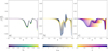 |
Fig. 8. Profile differences δtΓ1/Γ1 = [Γ1(t;Ys+δYs,ψCZ,ε)−Γ1(t;Ys,ψCZ,ε)]/Γ1 obtained for a fixed value of δYs = 0.05 and various sets (Ys, ψCZ, ε) (the values used here are not the same as those in Fig. 6) around the reference |

The situation in panel b is less intuitive. In order to provide realistic values for this rather uncommon parameter, we considered −9 < ψCZ < −3 as the electron degeneracy range, which corresponds to typical values inside solar-like oscillators (a justification of this point is provided later on). This time, the shape of the perturbation caused by a fixed change in the helium amount is very sensitive to the electron degeneracy value taken as a reference, and this highlights how counter-intuitive differences of profiles can be. At higher electron degeneracy levels, the perturbation looks like a more spread-out version of the perturbation visible in panel a, but its behaviour becomes more complex as the degeneracy decreases. Both helium wells lose their Gaussian aspect: the first well approaches a “heartbeat” shape, that is, it becomes clearly positive (probably under the influence of the hydrogen well), while the second well becomes progressively bi-modal. In contrast, the results in panel c could have been guessed from Fig. 6. The ε value shifts both reference and perturbed profiles, thus resulting in a scaled version of the perturbation shown in panel a.
As a consequence, Fig. 8 shows the issues inherent to calibration methods that we mentioned in Sect. 2. Even if it can be established that the choice of the helium amount Ys taken as reference does not ultimately matter greatly, Fig. 8 illustrates the diversity of δtΓ1/Γ1 profiles corresponding to the same helium difference by simply considering different values of ψCZ and ε. Reusing the notations introduced in Sect. 2, we clearly find that any change in a component of ⃗θ⋆ that may impact the best-fitting pair (ψCZ, ε)⊂⃗θp will lead to substantially different estimates of δY. In this respect, a parameter with a particularly strong impact is given in the forthcoming paragraphs, thus further distancing us from a unique relation of the form ⃗θp(δY) as assumed in Eq. (13). Furthermore, it should be added that the particular case of a perturbation around the reference value Ys = 0 (as considered in HG07) is no exception. Although we only varied the two remaining parameters ψCZ and ε, Fig. 9 shows the many possibilities for δtΓ1/Γ1 even when an identical helium difference δYs = 0.25 is considered from a pure hydrogen model Ys = 0. The spread of these randomly drown curves provides an idea of the potential dispersion of the perturbed profile at any point of the structure even under these “favourable” conditions.
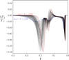 |
Fig. 9. Profile differences δtΓ1/Γ1 again obtained for a fixed value of δYs = 0.25, but from a pure-hydrogen reference model Ys = 0. The 500 profile differences in this plot were obtained by randomly drawing the remaining two reference quantities (ψCZ, ε) in the 2D box [ − 9, −3]×[0.015, 0.02] (the ε interval has been reduced compared to Fig. 8 for clarity). Two opposite corners of this box are highlighted in red and blue. |
Secondly, Figs. 8 and 9 underline how accustomed we are to conceive the structural perturbations caused by a variation in helium under solar conditions of electron degeneracy. We may note here the added value of having introduced a model physically; it would have been complicated to imagine and then parameterise these types of perturbations by simply observing a Γ1 profile in a realistic model. Accordingly, we may question the validity of using ad hoc profiles to approximate the perturbation caused by a change in helium abundance, and this particularly at low electron degeneracy (whose domain of relevance is discussed in the following). It appears to be likely that adjusting functions whose form is inappropriate for these complex profiles may result in inconsistencies regarding their parameterisations.
Up to this point, we only considered a given helium difference, in particular, to determine how the model presented in this paper agrees or contrasts with the types of perturbations for ionisation regions from previous studies. However, Eq. (73) clearly extends to the much more general difference
 (74)
(74)
When it applied to a frequency shift analysis, it appears to be unlikely that the model differs from its target in its helium abundance alone. We therefore propose to study the structural impact of a δψCZ or a δε difference below. It is obvious that the problems mentioned above in terms of the number of dependences will only be further amplified. For this reason, we fixed the reference set of parameters by taking for example the values  and varied the differences δYs, δψCZ, and δε one by one. The resulting profiles are shown in Fig. 10.
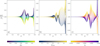 |
Fig. 10. Profile differences δtΓ1/Γ1 = [Γ1(t;Ys+δYs,ψCZ+δψCZ,ε+δε)−Γ1(t;Ys,ψCZ,ε)]/Γ1 obtained for a fixed reference parameter set (Ys, ψCZ, ε) = |

As expected, the variation observed in panel a is very similar to that in panel a of Fig. 8 scaled by a factor α = δYs/0.05. The other two perturbations, however, take different shapes and notably make the wells unrecognisable. A change in the electron degeneracy (panel b) has a strong impact on the hydrogen ionisation structure, especially at a point (t ∼ 0.09), where a change in helium has almost no effect. The ionisation region shift is also enhanced, while the second helium ionisation contributes to a weaker and more localised well. The variation in the position δε of the ionisation region is also fairly counter-intuitive. Panel c illustrates a contribution that reaches its maximum between the two helium wells (t ∼ 0.15), the one corresponding to the peak in the Γ1(t) profile.
Figure 10 highlights how elaborate the ionisation perturbation profile becomes in the general case. We recall that a structural perturbation from a reference  can be approximated as a combination of profiles composing Fig. 10. According to Eq. (74),
 (75)
(75)
with for instance
 (76)
(76)
being the structural perturbation studied in panel a within a multiplicative factor. With regard to Fig. 10, the result of the linear combination (75) can become highly complex and is unlikely to have anything in common with the functions generally used to fit δtΓ1/Γ1. Combined with the issues already raised about calibration, this tends to suggest that the study of the ionisation glitch based on ad hoc perturbation profiles in order to calibrate them afterwards might lead to fairly inconsistent results.
Moreover, we have tried to represent structural disturbances in the figure that are similar in order of magnitude. This allows us to qualitatively relate the values of the different parameters. In this sense, perturbations with δYs = 0.1, δψCZ = 1 or δε = 0.002 have a comparable structural impact in amplitude and hence on the frequencies. However, although the first impact nearly spans the entire range of relevant values (the difference in helium between two stars can hardly exceed 0.1), this is not the case for the two others. In the ε parameter, this change is very small: two consecutive curves in panel c of Fig. 6 are separated by exactly δε = 0.002, which is the entire span for the perturbation represented in Fig. 10. This last point suggests a very high dependence of the perturbation on a shift of the ionisation region. As mentioned above, it is interesting to note that the glitch signature would come from the Γ1 peak rather than from a well if this contribution were to dominate. This is consistent with observations that have been made in previous studies (Broomhall et al. 2014; Verma et al. 2014b), although it provides an alternative explanation.
To place the significance of a difference in the ψCZ parameter in perspective, it can be interesting to relate it to more intuitive quantities such as fundamental parameters. Because the electron degeneracy ψ is known to fluctuate with the mass of the star (e.g. Hayashi et al. 1962), we represent in Fig. 11 various ψ(t) profiles (along with the corresponding Γ1(t) profiles) obtained from CESTAM models of different masses. These models cover a wide range of values from 0.7 M⊙ to 1.35 M⊙ appropriate for solar-like pulsators. All the models also share the same composition (the solar composition) and subsequently the same helium abundance as well as the same evolutionary state (Xc = 0.6). Clearly, although their composition is identical, these models show fairly distinct Γ1(t) profiles in the ionisation region. The behaviour of these curves is fairly similar to that of the curves shown in panel b of Fig. 6 (which can be extrapolated to the wider range 0.45 M⊙ < M < 1.5 M⊙ presented as dashes as an indication). Thus, at low masses, the wells seem to merge and then split at higher masses, which in particular makes the HeI well visible. In addition to this effect, an expansion and contraction of the profiles is visible depending on the considered mass range (< 1 M⊙ or > 1 M⊙, cf. arrows shown in panels a and b). From examination of the similarities with Fig. 6, we interpret these changes as manifestations of variations in ε and the electron degeneracy just below the ionisation region. Although the variations of ε can only be evaluated qualitatively (we recall that this quantity is only defined in entirely convective models), this is not the case for the electron degeneracy. The ψ(t) profiles typically undergo little to no variation in convection zones, as shown by the plateaus in the curves in panel c, thus making it easy to identify ψCZ. The range of ψCZ values covered by these plateaus corresponds to the range studied in Fig. 8 (∼ − 3 for 0.7 M⊙ stars and ∼ − 9 for the 1.35 M⊙ model). It is then possible to seek to characterise the significance of the change δψCZ = 1 mentioned above. To provide an order of magnitude, we represent in panel c the ψ span corresponding to the mass uncertainty (1.14 < M* < 1.32) of HD 52265 taken from Lebreton & Goupil (2014). This star provides an example of a seismically determined mass uncertainty, taking into account a large number of biases as discussed in Sect. 1. The corresponding extent in terms of electron degeneracy is about δψCZ ∼ 2, which is twice larger than the range considered in panel b of Fig. 10 and thus larger than any possible variation in helium abundance. This range in ψCZ depends on the mass; this mass difference would correspond to a lower δψCZ at 0.7 M⊙ and would instead increase at higher masses. In this regard, a mass difference between two models could contribute to a perturbation of the structure of the ionisation region as large as (if not larger than) that of helium. Here, we note that a change in mass in a given evolutionary state has been studied. The impact of an age difference at a given mass has also been examined, which leads to smaller changes in both ψCZ and ε under the constraints provided by Lebreton & Goupil (2014). The only substantial variation in the Γ1 profile occurs in the 1.5 M⊙ model, with the appearance of a convective surface zone for Xc ≤ 0.4.
 |
Fig. 11. Γ1(t) (both panels a & b for clarity) and ψ(t) (panel c) profiles extracted from CESTAM early main sequence models with masses ranging from 0.7 M⊙ to 1.35 M⊙ (and from 0.45 M⊙ to 1.5 M⊙ as an indication in dashes). All models share the same composition which is the solar one as well as the same evolutionary state: Xc = 0.6. The qualitative variations of ε with mass are represented as well as the ψ span corresponding to the mass uncertainty of HD 52265 taken from Lebreton & Goupil (2014). |
Finally, to further echo the point made in Fig. 8 about calibration, the mass taken as a reference, M⋆, provides a representative example of a component of ⃗θ⋆ that impacts the (ψCZ, ε) pair, as already observed by Verma et al. (2014b). In this article, the authors proposed to use it by considering different calibrations to determine the helium abundance of stars of distinct masses. However, besides the fact that this presupposes a relatively good knowledge of the star in question before its helium abundance can be estimated, and we also saw that stars whose masses are already seismically constrained can possess significantly different degeneracy levels in the convective region. Using the example of HD 52265, the question then arises whether it is possible to obtain consistent results using calibration and being able to consider both models with ψCZ ∼ 6 or ψCZ ∼ 8, which implies perturbation profiles that differ in form and magnitude for a fixed difference in helium amount (see panel b of Fig. 8). This statement does not apply exclusively to the mass, M⋆, but can reasonably be extended to any fundamental parameters or physical processes (i.e., the other components of ⃗θ⋆) that may affect the average density in the convection zone (related to ψCZ) or the relative acoustic depth of the ionisation region (linked to ε).
In addition to this last remark, it appears likely by comparing the structural perturbations in Fig. 10 that the component caused by a helium change between two stars does not contribute alone. It might even be dominated by a change in electron degeneracy or in the ionisation region position. From the perspective of frequency shifts, it thus seems incorrect to assimilate the ionisation glitch as a repercussion of a helium difference only in order to infer its value. In this light, it appears essential to study forms of frequency shifts that can take these additional dependences into account, thus relying on physical models as proposed in this paper.
6. Conclusion
Determining abundances can be subject to many biases in its classical approach, which we intend to overcome by exploiting the ionisation glitch. However, although it progressively becomes more sophisticated, the glitch-based approach faces problems inherent to its current modelling, such as the need for calibration by realistic stellar models.
To address these problems, a physical model of the ionisation region was proposed here, explicitly involving the parameters of interest, such as the surface helium abundance Ys, and which can be generalised to more elaborate compositions. In the case of a hydrogen-helium mixture, the model involves three parameters and highlights the importance of characterising the electron degeneracy state in the convective zone ψCZ as well as the position of the ionisation region here controlled by ε. While it is well known that the abundance of surface helium contributes greatly to the appearance of the first adiabatic exponent (Γ1) profile by shaping the size of the helium wells, the state of degeneracy seems to affect the profile just as much by altering their dispersion. Taking this into consideration, the model is thus able to describe a wide variety of ionisation structures while providing them with a physical meaning. By comparing them to a CESTAM model, we also verified that it was able to approach realistic Γ1 profiles for consistent parameter values, which confers a predictive capacity to the model.
The modelling work we conducted allowed us to study the shape of structural perturbations by analysing differences of profile with distinct parameterisations. In particular, the form of the perturbations caused by a helium difference was addressed. Expected shapes were found, such as a Gaussian-like contribution for the helium ionisation regions with an additional sharper component at the surface, caused by a shift in the hydrogen ionisation region. However, we have observed that this form is only valid for a restricted case, namely a helium difference under solar electron degeneracy conditions. This perturbation appears to be highly variable with respect to these conditions, however, and can easily become much more complex at lower electron degeneracies. This point in particular stresses the major dependence of the perturbation on the choice of realistic models chosen for calibration purposes. We then proceeded to study more general parameter differences. More elaborate forms of perturbations than those usually assumed are found. We also suggested that there is a stronger dependence on the electron degeneracy in the CZ or on the position of the ionisation region than on the helium amount itself. Furthermore, the connection between electron degeneracy and stellar mass therefore enables us to clarify the strong dependence of the helium glitch amplitude on the stellar mass already observed by Verma et al. (2014b, 2019). Moreover, the fluctuation in the ionisation region position thus induced seems compatible with a glitch signature coming from the peak of the first adiabatic exponent as reported by Broomhall et al. (2014) or Verma et al. (2014b).
When analysing the oscillation frequencies, we therefore emphasise the importance of having a relation that can take these additional dependences into account. In this sense, a second paper based on the introduced modelling is planned in order to derive more general forms of frequency shifts. The objective should be to interpret the ionisation glitch as a combination of multiple contributions for which a variation of helium abundance is one component among others.
Convection, Rotation et Transits planétaires.
Transiting Exoplanet Survey Satellite.
References
- Antia, H. M., & Basu, S. 1994, A&AS, 107, 421 [NASA ADS] [Google Scholar]
- Asplund, M., Grevesse, N., Sauval, A. J., & Scott, P. 2009, ARA&A, 47, 481 [NASA ADS] [CrossRef] [Google Scholar]
- Baglin, A., Auvergne, M., Barge, P., et al. 2006, in The CoRoT Mission Pre-Launch Status - Stellar Seismology and Planet Finding, eds. M. Fridlund, A. Baglin, J. Lochard, & L. Conroy, ESA SP, 1306, 33 [NASA ADS] [Google Scholar]
- Baker, N., & Kippenhahn, R. 1962, Z. Astrophys., 54, 114 [NASA ADS] [Google Scholar]
- Ball, W. H., & Gizon, L. 2014, A&A, 568, A123 [NASA ADS] [CrossRef] [EDP Sciences] [Google Scholar]
- Ballot, J., Turck-Chièze, S., & García, R. A. 2004, A&A, 423, 1051 [NASA ADS] [CrossRef] [EDP Sciences] [Google Scholar]
- Basu, S., & Antia, H. M. 2004, ApJ, 606, L85 [NASA ADS] [CrossRef] [Google Scholar]
- Basu, S., Antia, H. M., & Narasimha, D. 1994, MNRAS, 267, 209 [NASA ADS] [CrossRef] [Google Scholar]
- Belkacem, K., Kupka, F., Samadi, R., & Grimm-Strele, H. 2019, A&A, 625, A20 [EDP Sciences] [Google Scholar]
- Belkacem, K., Kupka, F., Philidet, J., & Samadi, R. 2021, A&A, 646, L5 [NASA ADS] [CrossRef] [EDP Sciences] [Google Scholar]
- Broomhall, A. M., Miglio, A., Montalbán, J., et al. 2014, MNRAS, 440, 1828 [NASA ADS] [CrossRef] [Google Scholar]
- Canuto, V. M. 1997, ApJ, 482, 827 [Google Scholar]
- Christensen-Dalsgaard, J., Dappen, W., & Lebreton, Y. 1988, Nature, 336, 634 [Google Scholar]
- Christensen-Dalsgaard, J., Proffitt, C. R., & Thompson, M. J. 1993, ApJ, 403, L75 [Google Scholar]
- Christensen-Dalsgaard, J., & Thompson, M. J. 1997, MNRAS, 284, 527 [NASA ADS] [Google Scholar]
- Cox, J. P., & Giuli, R. T. 1968, Principles of Stellar Structure [Google Scholar]
- Deal, M., Alecian, G., Lebreton, Y., et al. 2018, A&A, 618, A10 [NASA ADS] [CrossRef] [EDP Sciences] [Google Scholar]
- Dziembowski, W. A., Pamyatnykh, A. A., & Sienkiewicz, R. 1990, MNRAS, 244, 542 [NASA ADS] [Google Scholar]
- Farnir, M., Dupret, M. A., Salmon, S. J. A. J., Noels, A., & Buldgen, G. 2019, A&A, 622, A98 [NASA ADS] [CrossRef] [EDP Sciences] [Google Scholar]
- Gilliland, R. L., Brown, T. M., Christensen-Dalsgaard, J., et al. 2010, PASP, 122, 131 [Google Scholar]
- Gough, D. O. 1990, in Progress of Seismology of the Sun and Stars, Proceedings of the Oji International Seminar Held at Hakone, Japan, 11–14 December 1989, eds. Y. Osaki, & H. Shibahashi (Berlin Heidelberg New York: Springer-Verlag), Lecture Notes Phys., 367, 283 [Google Scholar]
- Gough, D. O. 2002, in Stellar Structure and Habitable Planet Finding, eds. B. Battrick, F. Favata, I. W. Roxburgh, & D. Galadi, ESA SP, 485, 65 [NASA ADS] [Google Scholar]
- Gough, D. O., & Thompson, M. J. 1991, The Inversion Problem (Tucson: University of Arizona Press), 519 [Google Scholar]
- Hayashi, C., Hōshi, R., & Sugimoto, D. 1962, Prog. Theor. Phys. Suppl., 22, 1 [NASA ADS] [CrossRef] [Google Scholar]
- Houdek, G., & Gough, D. O. 2007, MNRAS, 375, 861 [CrossRef] [Google Scholar]
- Houdek, G., & Gough, D. O. 2011, MNRAS, 418, 1217 [NASA ADS] [CrossRef] [Google Scholar]
- Kippenhahn, R., Weigert, A., & Weiss, A. 2012, Stellar Structure and Evolution, 2nd Edition (Berlin Heidelberg: Springer-Verlag) [CrossRef] [Google Scholar]
- Kjeldsen, H., Bedding, T. R., & Christensen-Dalsgaard, J. 2008, ApJ, 683, L175 [Google Scholar]
- Kosovichev, A. G., Christensen-Dalsgaard, J., Daeppen, W., et al. 1992, MNRAS, 259, 536 [NASA ADS] [CrossRef] [Google Scholar]
- Lebreton, Y., & Goupil, M. J. 2014, A&A, 569, A21 [NASA ADS] [CrossRef] [EDP Sciences] [Google Scholar]
- Lopes, I., Turck-Chieze, S., Michel, E., & Goupil, M.-J. 1997, ApJ, 480, 794 [NASA ADS] [CrossRef] [Google Scholar]
- Lund, M. N., Silva Aguirre, V., Davies, G. R., et al. 2017, ApJ, 835, 172 [Google Scholar]
- Marques, J. P., Goupil, M. J., Lebreton, Y., et al. 2013, A&A, 549, A74 [NASA ADS] [CrossRef] [EDP Sciences] [Google Scholar]
- Monteiro, M. J. P. F. G., & Thompson, M. J. 1998, in New Eyes to See Inside the Sun and Stars, eds. F. L. Deubner, J. Christensen-Dalsgaard, & D. Kurtz, IAU Symp., 185, 317 [NASA ADS] [CrossRef] [Google Scholar]
- Monteiro, M. J. P. F. G., & Thompson, M. J. 2005, MNRAS, 361, 1187 [NASA ADS] [CrossRef] [Google Scholar]
- Monteiro, M. J. P. F. G., Christensen-Dalsgaard, J., & Thompson, M. J. 1994, A&A, 283, 247 [NASA ADS] [Google Scholar]
- Morel, P., & Lebreton, Y. 2008, Ap&SS, 316, 61 [Google Scholar]
- Mosumgaard, J. R., Jørgensen, A. C. S., Weiss, A., Silva Aguirre, V., & Christensen-Dalsgaard, J. 2020, MNRAS, 491, 1160 [Google Scholar]
- Noll, A., Deheuvels, S., & Ballot, J. 2021, A&A, 647, A187 [EDP Sciences] [Google Scholar]
- Nsamba, B., Campante, T. L., Monteiro, M. J. P. F. G., et al. 2018, MNRAS, 477, 5052 [NASA ADS] [CrossRef] [Google Scholar]
- Perez Hernandez, F., & Christensen-Dalsgaard, J. 1994, MNRAS, 269, 475 [NASA ADS] [CrossRef] [Google Scholar]
- Ricker, G. R., Winn, J. N., Vanderspek, R., et al. 2015, J. Astron. Telescopes Instruments Systems, 1, 014003 [Google Scholar]
- Rogers, F. J. 1981, Phys. Rev. A, 24, 1531 [NASA ADS] [CrossRef] [Google Scholar]
- Rogers, F. J., Swenson, F. J., & Iglesias, C. A. 1996, ApJ, 456, 902 [Google Scholar]
- Schou, J., & Birch, A. C. 2020, A&A, 638, A51 [NASA ADS] [CrossRef] [EDP Sciences] [Google Scholar]
- Serenelli, A. M., Basu, S., Ferguson, J. W., & Asplund, M. 2009, ApJ, 705, L123 [Google Scholar]
- Sonoi, T., Samadi, R., Belkacem, K., et al. 2015, A&A, 583, A112 [NASA ADS] [CrossRef] [EDP Sciences] [Google Scholar]
- Stassun, K. G., Oelkers, R. J., Paegert, M., et al. 2019, AJ, 158, 138 [Google Scholar]
- Tassoul, M. 1980, ApJS, 43, 469 [Google Scholar]
- Verma, K., Faria, J. P., Antia, H. M., et al. 2014a, ApJ, 790, 138 [Google Scholar]
- Verma, K., Antia, H. M., Basu, S., & Mazumdar, A. 2014b, ApJ, 794, 114 [NASA ADS] [CrossRef] [Google Scholar]
- Verma, K., Raodeo, K., Antia, H. M., et al. 2017, ApJ, 837, 47 [NASA ADS] [CrossRef] [Google Scholar]
- Verma, K., Raodeo, K., Basu, S., et al. 2019, MNRAS, 483, 4678 [Google Scholar]
Appendix A: Further simplifications and perturbation of the first adiabatic exponent
A.1. Deriving Eq. (53)
This parts details the derivation of (53) and (54) from (48)-(52). We first introduce the notation
 (A.1)
(A.1)
Equations (50)-(52) can then be rewritten as
 (A.2)
(A.2)
 (A.3)
(A.3)
 (A.4)
(A.4)
Injecting this into Eq. (48) then leads to
 (A.5)
(A.5)
and since
 (A.6)
(A.6)
we obtain the following expression, in which 5/3 appears, as expected:
 (A.7)
(A.7)
The simplifications in the numerator lead to the following more compact expression:
 (A.8)
(A.8)
We study the term χ2χ0 − (χ1)2,
![Mathematical equation: $$ \begin{aligned} \chi _2\chi _0-\left(\chi _1\right)^2&= \sum _{ijrs}x_ix_jy_i^ry_j^s\frac{(1-y_i^r)(1-y_j^s)\chi _i^r(\chi _i^r-\chi _j^s)/(kT)^2}{\left[1+\delta _i^1(1-y_i^r)\right]\left[1+\delta _j^1(1-y_j^s)\right]} \nonumber \\&= \sum _{ir<js}x_ix_jy_i^ry_j^s\frac{(1-y_i^r)(1-y_j^s)(\chi _i^r-\chi _j^s)^2/(kT)^2}{\left[1+\delta _i^1(1-y_i^r)\right]\left[1+\delta _j^1(1-y_j^s)\right]} \nonumber \\&< \sum _{ir < js}x_ix_jy_i^ry_j^s(1-y_i^r)(1-y_j^s)\left(\frac{\chi _i^r-\chi _j^s}{kT}\right)^2 ,\end{aligned} $$](/articles/aa/full_html/2021/11/aa41711-21/aa41711-21-eq173.gif) (A.9)
(A.9)
where we grouped the symmetrical terms under the notation ir < js. Most of the terms in this sum are negligible compared with the denominator, which is always greater than 3/2. Several effects contribute to keeping these terms small:
-
In order for the product xixj to contribute to the total, the number abundances of the two elements, i and j, needs to be non-negligible. Accordingly, the only non-negligible terms are those coupled to hydrogen.
-
The ionisation regions (i, r) and (j, s) should overlap as much as possible because otherwise
 would be null. Even in the most favourable case, we have the upper limit
  .
. -
At the same time, ionisation regions that overlap tend to have a similar ionisation potential, thus making
 small.
 -
As discussed in Section 3, ionisation regions are more likely to merge at higher conditions of temperature and density. However, in this case, 1/(kT)2 tends rapidly towards 0.
All these points appear to be arguing in favour of a small χ2χ0 − (χ1)2, and we confirm numerically that this term remains below 2 × 10⁻³ at any position of the (ρ, T) plane. We thus considered that χ2χ0 − (χ1)2 = 0 for the remainder of our derivation. Eq. (53) quickly ensues by introducing
 (A.10)
Relation (54) is simply obtained by replacing χ2 by its definition (A.1). Eq. (A.4) shows  , and this results in the property stated in the main part, namely 0 ≤ γ1 < 1, or equivalently, 1 < Γ1 ≤ 5/3.
A.2. Perturbing Γ1 at given V, T values
The resulting relation, Eq. (A.10), is so compact that we can perturb it analytically in terms of abundances (which was not an option when considering Eq. (48)). We consider a change δxi of the xi at given V and T values (with the implicit condition ∑iδxi = 0). Considering Eqs. (32)-(34), the  thus defined are functions of T and V, but not of xi. It can thus be established that
  . The induced perturbations of χ2 and
  is therefore given by
 (A.11)
 (A.12)
thus leading to the following impact on γ1:
 (A.13)
By calculating the numerator explicitly, four sums appear,
![Mathematical equation: $$ \begin{aligned} \begin{aligned} (\partial _{TT}^2f)^2 \delta _{V,T}(\gamma _1) ~&=~ \frac{3}{2}\sum _{ir} \frac{\delta x_i}{x_i} x_i y_i^r(1-y_i^r)\frac{{(\chi _i^r/kT)}^{2}}{1+\delta _i^1(1-y_i^r)}\\ + \frac{3}{2}&\sum _{ijrs}\left(\frac{\delta x_i}{x_i}-\frac{\delta x_j}{x_j}\right)x_ix_jy_i^ry_j^s\frac{(1-y_i^r)(\chi _i^r/kT)^2}{1+\delta _i^1(1-y_i^r)}\\ + \frac{9}{4}\sum _{ijrs} \frac{\delta x_i}{x_i}&x_ix_jy_i^ry_j^s\frac{(1-y_i^r)(1-y_j^s)(\chi _i^r+\chi _j^s)(\chi _i^r-\chi _j^s)/(kT)^2}{\left[1+\delta _i^1(1-y_i^r)\right]\left[1+\delta _j^1(1-y_j^s)\right]}\\ + 3\sum _{ijrs} \frac{\delta x_i}{x_i}&x_ix_jy_i^ry_j^s\frac{(1-y_i^r)(1-y_j^s)\chi _i^r\chi _j^s(\chi _i^r-\chi _j^s)/(kT)^3}{\left[1+\delta _i^1(1-y_i^r)\right]\left[1+\delta _j^1(1-y_j^s)\right]} \end{aligned} .\end{aligned} $$](/articles/aa/full_html/2021/11/aa41711-21/aa41711-21-eq185.gif) (A.14)
(A.14)
If we group symmetrical terms, the last two sums are bounded by
 (A.15)
and
 (A.16)
For the same reasons as mentioned above, we consider that these two terms are negligible in the following. Because δV, T(Γ1) = − 2/3δV, T(γ1), an analytical expression of the perturbation is given by
![Mathematical equation: $$ \begin{aligned} \delta _{V,T}(\Gamma _1) ~\simeq ~ -\frac{1}{(\partial _{TT}^2f)^2}&\sum _{ir} x_i y_i^r\frac{(1-y_i^r){(\chi _i^r/kT)}^{2}}{1+\delta _i^1(1-y_i^r)}\nonumber \\&\quad \left[\frac{\delta x_i}{x_i}+\sum _{js}x_jy_j^s\left(\frac{\delta x_i}{x_i}-\frac{\delta x_j}{x_j}\right)\right]. \end{aligned} $$](/articles/aa/full_html/2021/11/aa41711-21/aa41711-21-eq188.gif) (A.17)
(A.17)
A.3. Perturbing Γ1 at given ρ, T values
The perturbation at given ρ and T values is more complex because  because of the variable change ρ/m0 = N/V. For any quantity α, the resulting perturbation change can be found by applying
 (A.18)
The perturbation of any quantity expressed in terms of  can be found using
  . To simplify the derivation, we present only the parts that do not result in terms containing
  , which are neglected,
 (A.19)
The resulting perturbation of the numerator is approximated by
![Mathematical equation: $$ \begin{aligned} (\partial _{TT}^2f)^2 \delta _{\rho ,T}(\gamma _1) ~&=~ (\partial _{TT}^2f)^2 \delta _{V,T}(\gamma _1) + (\partial _{TT}^2f)^2\left[\delta _{\rho ,T}(\chi _2)-\delta _{V,T}(\chi _2)\right] \nonumber \\&~~~~~~~~~~~~~~~~~~~~~~~~~~~~~~~- (\chi _2)\left[\delta _{\rho ,T}(\partial _{TT}^2f)-\delta _{V,T}(\partial _{TT}^2f)\right] \nonumber \\ ~&\simeq ~ (\partial _{TT}^2f)^2 \delta _{V,T}(\gamma _1) + \frac{3}{2}(\partial _V f)\left[\delta _{\rho ,T}(\chi _2)-\delta _{V,T}(\chi _2)\right] \nonumber \\ ~&\simeq ~ (\partial _{TT}^2f)^2 \delta _{V,T}(\gamma _1) \nonumber \\ + \frac{3}{2}\frac{\delta m_0}{m_0}&\sum _{ir} x_i y_i^r\left(\frac{(1-y_i^r)(\chi _i^r/kT)}{1+\delta _i^1(1-y_i^r)}\right)^2 \nonumber \\&\qquad \left(\frac{2-y_i^r}{1-y_i^r}+\frac{\delta _i^1y_i^r}{1+\delta _i^1(1-y_i^r)}\right)\left(1+\sum _{js}x_jy_j^s\right). \end{aligned} $$](/articles/aa/full_html/2021/11/aa41711-21/aa41711-21-eq195.gif) (A.20)
(A.20)
Finally, the overall perturbation on δρ, T(Γ1) is given by the two sums
![Mathematical equation: $$ \begin{aligned} \delta _{\rho ,T}(\Gamma _1) ~\simeq ~ -\frac{1}{(\partial _{TT}^2f)^2}&\sum _{ir} x_i y_i^r\frac{(1-y_i^r){(\chi _i^r/kT)}^{2}}{1+\delta _i^1(1-y_i^r)} \nonumber \\&\qquad \left[\frac{\delta x_i}{x_i}+\sum _{js}x_jy_j^s\left(\frac{\delta x_i}{x_i}-\frac{\delta x_j}{x_j}\right)\right] \nonumber \\ -\frac{\delta m_0/m_0}{(\partial _{TT}^2f)^2}&\sum _{ir} x_i y_i^r\left(\frac{(1-y_i^r)(\chi _i^r/kT)}{1+\delta _i^1(1-y_i^r)}\right)^2 \nonumber \\&\qquad \left(\frac{2-y_i^r}{1-y_i^r}+\frac{\delta _i^1y_i^r}{1+\delta _i^1(1-y_i^r)}\right)\left(1+\sum _{js}x_jy_j^s\right) . \end{aligned} $$](/articles/aa/full_html/2021/11/aa41711-21/aa41711-21-eq196.gif) (A.21)
(A.21)
Although we have neglected many terms to obtain Eq. (A.21), this equation still gives a useful approximation. For instance, the difference between Γ1(ρ, T, 0.35)−Γ1(ρ, T, 0.25) (shown in Fig. 5) and the relation (A.21) is bounded by 10−2 at any position of the (ρ, T) plane, and we verify that panel (b) of Fig. A.1 is very similar to what we found in panel (d) of Fig. 5. We also represent the perturbation given by (A.17), which appears to be closer to the shape that can be expected for the perturbation, at least based on panel (b) of Figure 5. The fact that the perturbation moves towards the borders of each ionisation region when it passes from δV, T(Γ1) to δρ, T(Γ1) is then interpreted as the result of a shift in  caused by perturbing at constant ρ. In other words, at a given density, a perturbation on the abundances causes the ionisation regions to move, and this results in a less intuitive map. This effect can be seen as artificial, however, because it is obtained by fixing a variable that mixes the specific effects of various state variables (i.e. V and each Ni).
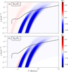 |
Fig. A.1. Representation of the approximations (A.17) (panel (a)) and (A.21) (panel (b)) given by a change δY = 0.1 from the reference value Y = 0.25. |
To give a qualitative understanding of the amplitude difference between the modification of the hydrogen and helium wells shown in the top panel of Fig. A.1, we may consider the dominant term of the denominator in Eq. (A.17),
 (A.22)
where the  notation stands for the dominant term in the ionisation region (i, r). Comparing this with the numerator of Eq. (A.17) gives an intuition of why the order of magnitude to keep in mind for the perturbation is δxi/xi rather than δxi. Thus, while we have δx1 = −δx2 for the hydrogen-helium case, we see that δx1/x1 = −δx2/x1 = −(x2/x1)δx2/x2. However, for Y = 0.25, (x2/x1) = 1/12, resulting in a perturbation about 12 times lower in the hydrogen region. This estimate is consistent with Fig. A.1, where the maximum in the hydrogen region is ∼6 × 10⁻³ and the minimum in the helium region ∼ − 7.2 × 10⁻².
All Tables
Inferred electron degeneracy parameter and helium abundance and actual CESTAM quantities.
All Figures
|
Fig. 1. Schematic illustration of several potential biases involved in the inference problem. Applied to the abundance determination problem, the observable space represents (notably) the oscillation frequency sets, while the unobservable space would represent the model abundances. Case a shows an ideal scenario, where for given constraints (blue circle) our modelling (in grey) provides unbiased abundances (red circle). Panel b: possible expression of physical processes that are missing or are poorly taken into account in the model. It thus results in physical biases although it has ideal observables. Case c provides an example of degeneracy, that is, parameters that can vary widely because they are too weakly constrained by the observables. The last panel d is a typical illustration of the solar problem, where no mixture seems to satisfy the constraints. In this case, inconsistencies in the model physics or much weaker constraints than actually provided by the oscillation frequencies must be considered in order to provide a solution. |
| In the text | |
|
Fig. 2. Various shapes along with their associated parameters that are used to describe a structural perturbation. (a) Dirac function used in Monteiro et al. (1994) to model the variations in the acoustic potential (in the case of an overshoot) passing from a convective to a radiative region. For this modelling, it is only necessary to specify the acoustic depth τd and amplitude Aδ of the perturbation. (b) Triangular shape of the Γ1 perturbation in the second helium ionisation region as used in Monteiro & Thompson (2005). An additional parameter controls the width (β) of the perturbation. (c) Gaussian shape of the Γ1 perturbation in the second helium ionisation region as used in Houdek & Gough (2007). |
| In the text | |
|
Fig. 3. Representation of a typical Γ1 profile in the ionisation region as a function of the acoustic depth τ (the surface corresponds to τ = 0). The helium abundance in this plot is Y ∼ 0.25. The contributions of the three main ionisation zones have been distinguished, i.e., the hydrogen (H), the first (HeI), and second (HeII) helium ionisation zones. Each of them causes a deviation from the Γ1 reference value of 5/3. |
| In the text | |
|
Fig. 4. Comparison of approximations (33) and (34) in the case i = 1, 2 (opaque curves) with the numerical solution of (26) (dashed light curves) for solar near-surface conditions of (T, V, Xi > 1). These quantities are represented as a function of the normalised acoustic depth t = τ/τ0 (the surface is then located at t = 0), along which all future plots are represented. |
| In the text | |
|
Fig. 5. 2D maps of the first adiabatic exponent obtained from Eq. (53). Panels a–c: Γ1(ρ, T, Y) as a function of ρ and T for different values of Y. Panel d: variation δρ, TΓ1 caused by a perturbation δY = 0.1 from a reference value Y = 0.25. The dashed line in each panel shows the relation ρ(T) extracted from a CESTAM solar model. |
| In the text | |
|
Fig. 6. Γ1(t) profiles obtained by considering various sets (Ys, ψCZ, ε) around a reference |
| In the text | |
|
Fig. 7. Correspondence between the CESTAM profiles and their respective analogues in our model. (a) Comparison of |
| In the text | |
|
Fig. 8. Profile differences δtΓ1/Γ1 = [Γ1(t;Ys+δYs,ψCZ,ε)−Γ1(t;Ys,ψCZ,ε)]/Γ1 obtained for a fixed value of δYs = 0.05 and various sets (Ys, ψCZ, ε) (the values used here are not the same as those in Fig. 6) around the reference |
| In the text | |
|
Fig. 9. Profile differences δtΓ1/Γ1 again obtained for a fixed value of δYs = 0.25, but from a pure-hydrogen reference model Ys = 0. The 500 profile differences in this plot were obtained by randomly drawing the remaining two reference quantities (ψCZ, ε) in the 2D box [ − 9, −3]×[0.015, 0.02] (the ε interval has been reduced compared to Fig. 8 for clarity). Two opposite corners of this box are highlighted in red and blue. |
| In the text | |
|
Fig. 10. Profile differences δtΓ1/Γ1 = [Γ1(t;Ys+δYs,ψCZ+δψCZ,ε+δε)−Γ1(t;Ys,ψCZ,ε)]/Γ1 obtained for a fixed reference parameter set (Ys, ψCZ, ε) = |
| In the text | |
|
Fig. 11. Γ1(t) (both panels a & b for clarity) and ψ(t) (panel c) profiles extracted from CESTAM early main sequence models with masses ranging from 0.7 M⊙ to 1.35 M⊙ (and from 0.45 M⊙ to 1.5 M⊙ as an indication in dashes). All models share the same composition which is the solar one as well as the same evolutionary state: Xc = 0.6. The qualitative variations of ε with mass are represented as well as the ψ span corresponding to the mass uncertainty of HD 52265 taken from Lebreton & Goupil (2014). |
| In the text | |
|
Fig. A.1. Representation of the approximations (A.17) (panel (a)) and (A.21) (panel (b)) given by a change δY = 0.1 from the reference value Y = 0.25. |
| In the text | |
Current usage metrics show cumulative count of Article Views (full-text article views including HTML views, PDF and ePub downloads, according to the available data) and Abstracts Views on Vision4Press platform.
Data correspond to usage on the plateform after 2015. The current usage metrics is available 48-96 hours after online publication and is updated daily on week days.
Initial download of the metrics may take a while.