| Issue |
A&A
Volume 655, November 2021
|
|
|---|---|---|
| Article Number | A116 | |
| Number of page(s) | 22 | |
| Section | Astronomical instrumentation | |
| DOI | https://doi.org/10.1051/0004-6361/202141458 | |
| Published online | 01 December 2021 | |
Spatial and temporal variations of the Chandra ACIS particle-induced background and development of a spectral-model generation tool⋆
1
Department of Physics, The University of Tokyo, 7-3-1 Hongo, Bunkyo-ku, Tokyo 113-0033, Japan
e-mail: hiromasa050701@gmail.com
2
Department of Physics, Faculty of Science and Engineering, Konan University, 8-9-1 Okamoto, Kobe, Hyogo 658-8501, Japan
3
Center for Astrophysics | Harvard & Smithsonian, 60 Garden Street, Cambridge, MA 02138, USA
4
Research Center for the Early Universe, The University of Tokyo, 7-3-1 Hongo, Bunkyo-ku, Tokyo 113-0033, Japan
Received:
28
May
2021
Accepted:
25
August
2021
Context. In X-ray observations, estimating the particle-induced background is important, especially for faint and/or diffuse sources. Although software exists to generate total (sky and detector) background data suitable for a given Chandra ACIS observation, no public software exists to model the particle-induced background separately.
Aims. We aimed to understand the spatial and temporal variations of the particle-induced background of Chandra ACIS obtained in the two data modes, VFAINT and FAINT.
Methods. Observations performed with ACIS in the stowed position shielded from the sky and the Chandra Deep Field South (CDF-S) data sets were used. The spectra were modeled with a combination of the instrumental lines of Al, Si, Ni, and Au and continuum components. The spatial variations of the spectral shapes were modeled by dividing each CCD into 32 regions in the CHIPY direction. The temporal variations of the spectral shapes were modeled using all the individual ACIS-stowed observations.
Results. Similar spatial variations of the spectral shapes were found in VFAINT and FAINT data, which are mainly due to the inappropriate correction of charge transfer inefficiency for events that convert in the frame-store regions. The temporal variation of the spectral hardness ratio is ∼10% maximum, which seems to be largely due to solar activity. We modeled this variation by modifying the spectral hardnesses according to the total count rate. Incorporating these properties, we developed a tool, mkacispback, to generate the particle-induced background spectral model corresponding to an arbitrary celestial observation. As an example application, we used the background spectrum produced by the mkacispback tool in an analysis of the unresolved cosmic X-ray background in the CDF-S observations. We found intensities of 3.10 (2.98–3.21)×10−12 erg s−1 cm−2 deg−2 in the 2–8 keV band and 8.35 (8.00–8.70)×10−12 erg s−1 cm−2 deg−2 in the 1–2 keV band, which are consistent with or lower than previous estimates.
Conclusions. We modeled the spatial and temporal variations of the particle-induced background spectra of the Chandra ACIS-I and the S1, S2, and S3 CCDs, and developed a tool to generate a spectral model for an arbitrary celestial observation.
Key words: methods: data analysis / instrumentation: detectors / X-rays: general
The tool mkacispback is available at https://github.com/hiromasasuzuki/mkacispback.
© ESO 2021
1. Introduction
For X-ray spectroscopy, background estimation is important especially for observations of faint and/or diffuse sources. For point sources, the background can be estimated from nearby regions that are free from the source emission. On the other hand, accurate background estimation from nearby regions is difficult for extended sources due to the contamination of the source emission and spatial variation of the background spectra. The background consists of the cosmic background from Galactic and extragalactic sources (hereafter “sky background”) and the background induced by cosmic-ray particles (hereafter “particle-induced background”). Both the observed sky and particle-induced backgrounds depend on the detector configuration and data reduction method. There have been many efforts to study and model the particle-induced background for individual detectors onboard satellites (e.g., Tawa et al. 2008 for Suzaku (XIS); Kuntz & Snowden 2008; Salvetti et al. 2017; Gastaldello et al. 2017; Marelli et al. 2021 for XMM-Newton (EPIC); Wik et al. 2014 for NuSTAR). These works provided sufficient information on how one should model the background in an arbitrary observation. The particle-induced background is complicated because many physical processes contribute to it, such as direct hits, the generation of secondary particles, fluorescence line emissions, and radioactivation. Thus, the particle-induced background in the X-ray energy range was treated phenomenologically except for a few recent studies based on detector simulations (e.g., Hagino et al. 2020 for the HXI onboard Hitomi and Lotti et al. 2017; Grant et al. 2020 for the X-IFU and WFI onboard Athena).
In general, the particle-induced background depends on the satellite position and attitude, and the solar activity. In the case of Suzaku, the particle-induced background is thought to be free from temporal variation of solar activity due to its low-earth orbit. The background spectra for an observation are thus determined by the satellite position and can be predicted from the Earth-occultation data obtained at the same satellite location. For XMM-Newton, because of its high altitude, the particle-induced background is highly affected by solar flares. Temporal variations of the flux and spectral shape of the background were found. In addition, spatial variations of the instrumental fluorescence lines were also found. One can model the detector background spectra using the data from the parts of the CCD that are shielded from focused X-rays from cosmic sources (Kuntz & Snowden 2008).
In the case of Chandra, most observers can extract a useful background region that is free from emission from the source given Chandra’s superb imaging capabilities. However, there are sources that are large enough to fill the entire Chandra field of view, and such an approach is not possible. For these cases, the Chandra X-ray Center (CXC) has made available the CALDB “blank-sky” data sets and software to create a background events list suitable for the observation of interest1. These blank-sky data sets include the sky and particle-induced background components as they are derived from Chandra pointings with point sources removed from various locations on the sky (Markevitch et al. 2003). Two disadvantages of this approach are that it combines the sky and particle-induced background components and it averages the sky background from different directions. For some applications, it would be advantageous to model the sky and particle-induced background components separately. This would require a model of the particle-induced background of the detector. Bartalucci et al. (2014) studied the spatial and temporal variation of the particle-induced background of the ACIS-I CCDs in the very faint (VFAINT) mode. They parameterized the spectra with multiple line components, a power-law, and an exponential function. The spatial variation was found to be largely due to the “frame-store lines” (“daughter lines” in Bartalucci et al. 2014), which are the emission lines detected in the frame-store regions of the ACIS array during frame readout (see, e.g., Fig. 1 for the position of the frame-store region). This variation was seen only along the readout direction as expected. The temporal variation, that is, the short-term variation depending on the satellite position and long-term variation due to the solar activity, was described by changing the normalizations of the spectra without changing their shapes.
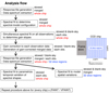 |
Fig. 1. Description of our analysis flow. The “stowed” and “blank-sky”, “merged” and “each obs.”, and “whole chip” and “32 slice regions” stand for the observation types, data types, and detector regions for which the analysis processes are applied, respectively. After the gain correction part, the “merged” and “each obs.” mean the gain-corrected-and-merged data and each of the gain-corrected observation data, respectively. A schematic drawing of a CCD chip with the 32 slice regions along CHIPY, readout direction, and frame-store region is also shown. |
This work aims to characterize the spatial and temporal variations of the particle-induced background spectra of the Chandra ACIS-I and S1, S2, and S3 CCDs obtained in both the FAINT and VFAINT modes, and to develop a spectral-model generation tool for practical uses. The data obtained in FAINT mode include higher particle-induced background contributions than those in VFAINT mode. Also, the back-illuminated (BI) CCDs have a higher event rate in the accepted grade set (g02346) due to particles than the FI CCDs owing to the fact that more of the particle events appear in the rejected grade set for the FI CCDs. These properties are suitable for a detailed study to investigate their spatial and temporal variations. Throughout the paper, errors indicate a 1 σ confidence range.
2. Data reduction and analysis
We used two types of data sets to obtain spectral models to describe the particle-induced background for ACIS: the “ACIS-stowed” observations and the Chandra Deep Field South observations (CDF-S blank-sky observations hereafter). The ACIS-stowed observations were conducted with ACIS out of the focal position of the telescope so that the events would originate only from the particle-induced background. The CDF-S blank-sky data sets consist of the sky background (unresolved Galactic and extragalactic sources) and particle-induced background. We note that this blank-sky data set is different from the CXC’s CALDB blank-sky data sets, which were only used for the verification of our background modeling as described in Sect. 4. We used the Chandra Deep Field South observations because they have longer exposures, hence the statistics are better. For the CDF-S blank-sky observations, we did not remove point sources from the field of view. Because we only used the CDF-S blank-sky data for the energies above 7 keV, the point sources contribute less than a few percent of the total counts (Bartalucci et al. 2014). The observation logs for each of these two data types are summarized in Tables A.1 and A.2. The ACIS-stowed observations range from 2002 to 2016, with a total exposure of ∼1 Ms. The CDF-S blank-sky observations range from 2007 to 2016, with a total exposure of ∼7 Ms. For each observation, the data were reprocessed to create a “level = 2” event file. In the analysis below, spectra, and corresponding response files are created based on the level = 2 files. The “merged” events files for each of the ACIS-stowed and CDF-S blank-sky data sets are generated as well by merging all the observations listed in Tables A.1 and A.2, respectively.
In the data reduction, we used CIAO (v4.11; Fruscione et al. 2006) and HEAsoft (v6.20; NASA HEASARC 2014). In the spectral analysis, we used XSPEC (v12.9.1; Arnaud 1996). The C-statistic, which has been implemented in XSPEC as cstat, is used in all the spectral fitting (Cash 1979; Kaastra 2017).
The overall analysis procedure is summarized in Fig. 1. Our approach for the spectral modeling is based on Bartalucci et al. (2014) and the presentation by T. Gaetz at the 14th IACHEC 20192. In the first step, the energy spectra and response matrices were generated for individual CCD chips for the ACIS-stowed observations. Using these, we generated a spectral model to describe the data. The resultant spectral model is a combination of multiple Gaussian lines and several continuum models (power-law, broken-power-law, and exponential function). The line components are composed of Al, Si, Au, and Ni lines. The line centroids are fixed to the literature values (Bearden et al. 1967) shown in Table 1. As described in Bartalucci et al. (2014), the spectra include broad line components produced by the inappropriate correction of charge transfer inefficiency (CTI) for events that convert in the frame-store regions of the CCDs (frame-store lines). The spectral shape of the frame-store line can be approximated by a function:
Detector line properties included in this work (Bearden et al. 1967).
where the C is a constant and Emin and Emax determine the boundaries of the component. Figure 2 shows an example of the merged ACIS-stowed and CDF-S blank-sky spectra extracted from a small region of the I0 CCD. The broad line components seen at ≈2.7 keV and ≈10.7 keV are the frame-store lines originating from Au-M and Au-L lines, respectively3. All the parameters of the model components other than the line centroids were treated as free parameters in our analysis.
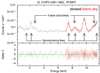 |
Fig. 2. Example spectrum of the observational particle-induced background extracted from a small region (CHIPX, CHIPY) = (1: 1024, 961: 992) of the I2 CCD. The data are extracted from the merged ACIS-stowed (black) and CDF-S blank-sky (red) observations. Upper and lower panels: present the fluxes and residuals, respectively. The data and the best-fit models are shown with the crosses and solid lines. The model components are presented with the dotted lines. We note that the spectral extraction region is far from the frame-store region so that the CTI effects are important. |
We note two things about our analysis. First, in the ACIS-stowed observations, only one observation (OBSID: 62678) for the I1 CCD is available. Thus, the spatial and temporal variations of the I1 data were substituted by those of the I0 data, given the expected similar properties4. This treatment is the same as that of Bartalucci et al. (2014). Second, the CDF-S blank-sky data are not available for the S1 and S3 CCDs. Although we found that spectral models for the S1 and S3 CCDs could be obtained only with the ACIS-stowed data, we also used the CALDB blank-sky data sets, which include the S1 and S3 CCD data, to verify these spectral models (Sect. 4).
2.1. Detector gain correction
In principle, the detector gains are well-calibrated in the level = 2 events files at energies between 1.5 and 6.0 keV given that these are the energies of the strongest lines in the calibration source onboard. At energies above 6.0 keV, the gain calibration may be less accurate and may lead to residuals around the strong lines of Ni at ≈7.5 keV and Au at ≈9.7 keV. In order to investigate the gain variations, we fitted the spectra extracted from individual observations simultaneously with the model configuration obtained above. The energy ranges of 0.25–11.5 keV for the ACIS-stowed and 7.0–11.5 keV for the CDF-S blank-sky spectra were used. The spectra were extracted from the entire CCDs. The energy range for the CDF-S blank-sky observations were selected based on Bartalucci et al. (2014) to avoid contamination of the sky background. We fitted the data with free gain offset and slope parameters, but found that the gain offset values were small (scatter by a few eV, typically, and are mostly consistent with zero). Thus, for the sake of the reduction of computational costs, only their slopes were treated as free parameters. An offset of zero and a small deviation from a slope of 1.0 is consistent with an accurate gain calibration below 6.0 keV and a small adjustment at energies above 6.0 keV. The gain slopes are constrained by the energy centroids of the line emissions, particularly by those of Ni-Kα and Au-Lα emissions.
The resultant gain slope values versus observation date are presented in Figs. 3 and 4. The gain values for VFAINT and FAINT modes are roughly consistent with each other. In some observations, slight inconsistencies are seen between them. These are probably due to high continua and thus less prominent line emissions in FAINT mode, which may lead to a less accurate estimation of the gain slopes. Generally, this level of the discrepancies will not affect the spectral modeling, but it might affect some cases, as discussed in Sect. 4. The I3 and S2 CCDs were found to show relatively stable gain slopes with time, whereas those of the I0, I2, and S1 CCDs vary greatly within ∼ ± 2%. We applied the gain correction to each observation based on the gain slopes obtained above and generated gain-corrected spectra and response matrices. Then, the gain-corrected-and-merged spectra were generated as well. For the S1 CCD in FAINT mode, the gains could not be determined because of the particularly high continuum, so no gain correction was applied to it.
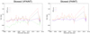 |
Fig. 3. Gain slopes for individual ACIS-stowed observation data. The S1 data obtained in FAINT mode are excluded because the gain slopes are not determined well in this case due to less prominent line emissions. |
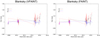 |
Fig. 4. Gain slopes for individual CDF-S blank-sky observation data. |
2.2. Spatial variation of the spectra
In Fig. 5, we present CHIPY-energy scatter plots for stowed events extracted from I0, I2, and I3 showing various X-ray fluorescence lines. The vertical features are fluorescent lines (Al-K, Si-K, Au-L, Ni-K, and Au-K) which convert in the imaging part of the array. The CHIPY-dependent CTI correction has been applied, which corrects for the decrease in pulse height amplitude (PHA) due to CTI. Many of these lines also have the frame-store lines, which are fainter lines associated with reported energies increasing with CHIPY. In processing the data, the software applies an energy- and CHIPY-dependent correction to the event PHAs. Because the frame store is undamaged by the radiation dose the FI chips experienced early in the mission, the CTI in the frame store is close to zero. The frame-store events effectively experience no CTI, so the application of the CTI correction results in an inappropriate increase in the frame-store event PHAs, giving an approximately linear variation of the frame-store line energies.
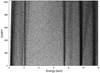 |
Fig. 5. Scatter plot of the particle-induced background events on the CHIPY-energy plane extracted from the merged ACIS-stowed data. This is the sum of the I0, I2, and I3 events. Darker regions include larger numbers of events. |
We investigated the CHIPY dependence of the frame-store line energies using an approach similar to that of Bartalucci et al. (2014) to determine the energy bounds of the frame-store lines. The event list reports for each event a “PHA_RO” (readout PHA, depending on the charge collected in the 3 × 3 event detection island), and PHA (the result after applying CTI correction). The ENERGY column provides the event energies, the result of adding a time-dependent gain (“TGAIN”) correction5, and the result when using the DETGAIN information. For clarity, we refer to the PHA_RO values as pharaw, the CTI-corrected PHA values as phacrt, and the ENERGY values as E. One can approximate the energy displacement of the frame-store events as
The CHIPY-ΔE plots for individual fluorescence frame-store lines show linear-like correlations with larger ΔE values at larger CHIPY values. An example is shown in Fig. 6, which shows the CHIPY versus ΔE variation for the Au-Lα2 line for the CCDs I0, I2, and I3. The red lines are linear fits for ΔE versus CHIPY plots. The I2 chip has a larger TGAIN correction, resulting in the fit intercepting the CHIPY = 0 axis at a visibly negative value for energy; all of the chips have negative offsets, but these are usually small. In principle, we can calculate the linear trend for ΔE and the energy bounds of the frame-store lines from the CHIPY-ΔE plots, which can be extracted from any (sufficiently long) celestial observation of interest. However, we found no significant variations in the CHIPY-ΔE plots among observations, and we can describe the spectra extracted from the whole-chip regions of any observation by an average model determined by the merged ACIS-stowed data (see Sect. 4 and Figs. C.1–C.10)6. As for spectral variations along CHIPX, only small (mostly less than a few percent) variations of the spectral shapes were found for all the ACIS-I and S1, S2, and S3 CCDs (as partly noted by Bartalucci et al. 2014), based on our analysis of the merged ACIS-stowed data. We note that the spatial variations of the FAINT data are similar to those of the VFAINT data – the differences mostly appear in the spectral continuum shapes.
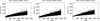 |
Fig. 6. Scatter plots of events on the CHIPY-ΔE plane for I0 (CCD0), I2 (CCD2), and I3 (CCD3). The events were extracted from the gain-corrected-and-merged ACIS-stowed data in VFAINT mode. The extraction energy range is 9.628 ± 0.2 keV. The red solid lines represent the best-fit linear functions. |
We extracted the data and response matrices for 32 slice regions along the CHIPY axis (see Fig. 7). These regions are defined as (CHIPX, CHIPY) = (1: 1024, 1: 32), (1: 1024, 33: 64), …, (1: 1024, 993: 1024). In order to model the spatial variations, we simultaneously fitted the gain-corrected-and-merged ACIS-stowed and CDF-S blank-sky spectra extracted from each slice region. As a validation of the fits, we confirmed here that each fitting result yields C-stat/d.o.f. < 1.1 (d.o.f. is ≈800–1100), where d.o.f. stands for degree of freedom. We repeated this process for the 32 regions for all CCDs used and both observation modes. An example of the spectral differences along CHIPY is shown in Fig. 7. Except for the difference in the detector responses, the largest difference is in the energy centroids and strengths of the frame-store lines. In this process, we treated all of the spectral parameters (including the energy bounds of the frame-store lines) other than the detector line centroids as free parameters. We obtained 32 sets of the model parameters for each CCD and each observation mode. These are the base models for the spectral-model generation tool described in Sect. 3.
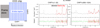 |
Fig. 7. Example of the spatial variation of the particle-induced background spectra. Two spectra extracted from the low- and high-CHIPY regions of the merged ACIS-stowed data (I0, VFAINT) are presented. Left panel: 32 slice regions along CHIPY. In each of the two right panels, the upper panel presents the data and model fluxes, whereas the lower panel presents their residuals. The black and red crosses represent the ACIS-stowed and CDF-S blank-sky observations, respectively. The solid and dotted lines are the total models and their components, respectively. |
2.3. Temporal variation of the flux and spectral shape
In this section, we investigate the temporal variations of the particle-induced background spectra. Figure 8 shows the long-term variation of the particle-induced background rate and its correlation with the solar activity (solar-flare rate)7. The left panel of Fig. 8 compares the temporal variation of the ACIS-stowed S3 count rate (0.25–11.5 keV) to an estimate of the total S3 cosmic-ray rate8. The S3 cosmic-ray rate is based on tallies of the “events” that exceed the S3 upper event PHA threshold (corresponding to event energies exceeding ≈12 keV). In the right panel of Fig. 8, a negative correlation between the particle-induced background and the solar activity is seen. This indicates that the temporal variation of the particle-induced background is largely due to solar activity, and thus the incoming cosmic-ray flux9.
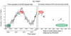 |
Fig. 8. Temporal variation of particle-induced background rate of ACIS-S3, FAINT mode. The transparent crosses are based on the rate of S3 events rejected onboard for exceeding the upper-level PHA threshold; they are scaled by ≈2% to be compared to the particle-induced background rate. The red and green ellipses enclose the observations at especially high and low particle-induced background rates. MJD stands for modified Julian date. |
Comparing the spectral shapes of the data to the average models which were obtained by summing the 32 sets of the base models (corresponding to the 32 ΔCHIPY regions), we found that the continuum shape varies and thus the hardness ratio also varies, as noted by Bartalucci et al. (2014). Figure 9 exhibits the variation of the spectral shapes by comparing the data to our average models for two extreme observations, OBSIDs 62850 and 62810. OBSID 62850 had one of the lowest overall background rates and OBSID 62810 had one of the highest. Discrepancies between the spectral normalizations of the data and average models for ∼1.0–7.0 keV can be seen in Fig. 9. Figs. 10 and 11 show the temporal variation of the hardness ratio (7.0–9.0 keV/1.0–7.0 keV) for the ACIS-stowed observations in VFAINT and FAINT modes, respectively. The average models obtained above are plotted in Figs. 10 and 11 for comparison. The two BI CCDs show significant variation of the hardness ratio of ≲ ± 10%. The FI CCDs show no significant variations in spectral shape. The tendency of the hardness-ratio variation of the BI CCDs with time is similar to that of the total particle-induced background rate (see Fig. 8), implying that the cause of these shape variations is also related to the cosmic-ray flux.
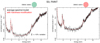 |
Fig. 9. Example of temporal variation of the particle-induced background spectral shapes. The black crosses represent the data. The black and red solid lines show the average spectral models and the models with the optimized hardness modification. We note that the OBSID 62850 and 62810 show the lowest and highest count rates in the ACIS-stowed observations, respectively. |
 |
Fig. 10. Hardness ratio (7.0–9.0 keV/1.0–7.0 keV) versus observation date. The black crosses and blue and red lines represent the data, average models, and models with the optimized hardness modification, respectively. The data and models are the ACIS-stowed observations processed in VFAINT mode. CCD 0, 2, 3, and 5–7 correspond to I0, I2, I3, and S1–S3, respectively. |
Here, we modeled the hardness-ratio variations only for the BI CCDs. As a simple model of this temporal variation of the spectral shapes, we let the continuum level in ≈1.0–7.0 keV (N1.0–7.0 keV) vary with respect to the other spectral components (let this be  ) depending on the count rate in 9.0–11.5 keV (R9.0–11.5 keV) as
where R0 and α are free parameters. Such a spectral variation is assumed to be due to the cosmic-ray spectral modulation in accordance with solar activity (e.g., Mizuno et al. 2004; Fiandrini et al. 2021), so this is assumed to depend on a total particle-induced background rate. The spectrum becomes harder in higher solar-activity periods, and this tendency is consistent with the cosmic-ray spectral modulation (e.g., Mizuno et al. 2004; Fiandrini et al. 2021). Applying this model, we fit all the ACIS-stowed observation spectra simultaneously to determine the best-fit R0 and α values for each CCD and each observation mode. The resultant parameter values are presented in Table 2. By applying this modification to the spectral models, we were able to better describe the observed hardness ratios (see Figs. 10 and 11) and actual spectral shapes (see Fig. 9), although this modeling was still not sufficient to fully explain the data.
The best-fit hardness-modification parameters α and β.
3. Design of the particle-induced background spectral-model generation tool, mkacispback
Based on the spectral model configurations and their spatial and temporal variation parameters obtained in Sect. 2, a tool named mkacispback was developed to generate the particle-induced background spectral model for an arbitrary observation10. We used the 32 spectral models for each CCD and each data mode as “template models” for the mkacispback tool. In addition, the temporal variation parameters R0 and α for each CCD and each observation mode were used.
A brief description of the steps executed by the tool is presented in Fig. 12. The input data are the (level 2) events file and the spectral extraction regions. First, in order to extract a particle-background count rate from the input region, it makes an image of the 9.0–11.5 keV energy band. Second, it makes a “weight map” by dividing the image into 32 × 32 regions per CCD. This weight map is converted to a vector that contains 32 values corresponding to the 32 template models by taking sums over CHIPX. Third, the total spectral model for one CCD is generated by taking a weighted-sum of the 32 template models based on this vector. After obtaining the spectral model for each CCD, in the fourth step, it modifies the spectral hardness based on the count rate in the 9.0–11.5 keV energy range. Fifth, the resultant spectral models for the CCDs covered by the region of interest are added together to obtain one spectral model. Finally, this spectral model is scaled to fit the data in the 9.0–11.5 keV energy range to produce the final output. The software is composed of shell scripts, Python (with the astropy library), C++, CIAO tools, and FTOOLS.
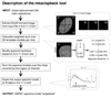 |
Fig. 12. Description of the process to generate the particle-induced background spectral model for arbitrary observation data, which are taken using the mkacispback tool. |
4. Verification of the mkacispback tool
4.1. Comparison to the ACIS-stowed and blank-sky observations
In order to check the validity of our tool, we first applied this tool to the gain-corrected-and-merged ACIS-stowed and CDF-S blank-sky data. For the S1 and S3 CCDs, because no data are available in the CDF-S blank-sky data set generated from the Chandra Deep Field South observations (Table A.2), we made use of the blank-sky data sets from CXC’s CALDB11. We combined the CALDB blank-sky observations that satisfy the conditions, focal plane temperature lower than −119°C, with CTI correction, and with TGAIN correction. Then we extracted the spectra in VFAINT and FAINT modes. The CALDB blank-sky data used in this work are summarized in Table 3.
CALDB blank-sky data list used in this work.
Figures 13 and 14 present the comparisons of the data and output spectral models of mkacispback for individual CCDs. To examine the modeling accuracy of mkacispback, we calculated the data-to-model ratio for the continuum regions (0.25–1.30 keV and 3.0–7.0 keV) and for the energies around strong lines (1.6–1.7 keV, 2.3–2.5 keV, 7.2–7.4 keV, and 9.2–9.6 keV). The modeling accuracy for the continuum and line regions was found to be within 5% and 8%, respectively. Judging from this, we conclude that the accuracy of the mkacispback tool is sufficient for most applications.
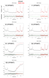 |
Fig. 13. Merged observational spectra obtained in VFAINT mode and the output spectral models of mkacispback. The spectra were extracted from the entire CCD regions. The S1 and S3 data were taken from the CALDB blank-sky data instead of the CDF-S blank-sky data set. For each CCD, the upper and lower panels represent the count rate and data-to-model ratio, respectively. We note that the background was higher in the period covered by the CALDB blank-sky observations, so offsets between the ACIS-stowed and CALDB blank-sky data are present. |
We note several things about Figs. 13 and 14. For the I1 CCD, although its spatial and temporal variations are parametrized with the same parameters as those for I0, the models represent the data rather well. At the energies below 0.7 keV, the S1 and S3 spectra in FAINT mode are higher than the models with discrepancies of ≲10%. This will be either due to insufficient spectral modeling in Sect. 2 or due to potential temporal or spatial variations, which have not been considered in this work. For several cases, such as the S3 FAINT at ≈1.8 keV and the I2 VFAINT around 9 keV, larger residuals of ≲10% can be seen around the line components, which are probably due to the insufficient gain corrections in Sect. 2. These residuals can be addressed in a future update of mkacispback. It is worth noting that the differences in count rates seen in Figs. 13 and 14 between the ACIS-stowed, and CDF-S blank-sky data are due to different particle background levels during the different time intervals of the data sets. The model does a reasonable job of estimating this difference, as seen in Figs. 13 and 14.
Figures C.1–C.10 present the comparison between individual ACIS-stowed observations and output models of mkacispback, to verify the model in more detail. The spectra were extracted from the entire CCD regions. As can be seen, for most cases, the models describe the data well without remarkable residual structures. For some cases, such as OBSIDs 62831, 62848, and 62850, relatively large residuals of ≲10% may be present even for their continuum regions. These may be due to our insufficient modeling of the temporal variations of the spectral shapes, which can be inferred from Figs. 10 and 11 as well. Future works may require detector simulations to understand the physical processes that are responsible for these variations.
4.2. Application to a celestial observation
As a demonstration of the application of mkacispback to actual celestial observations, we applied this tool to the X-ray emission of the supernova remnant G359.1−0.5, which is relatively old among supernova remnants and thus is a faint and diffuse source, where the particle-induced background is relatively important (e.g., Suzuki et al. 2020). An image of G359.1−0.5 is shown in the left panel of Fig. 15 with the spectral extraction region indicated by the green ellipse. The source spectrum with the background spectrum produced by mkacispback is shown in the right panel of Fig. 15. As well as the high-energy range of the 7.0–11.5 keV, the very low-energy part of ≲0.5 keV also shows a reasonable match between the data and model. We show an example application for an observation of a supernova remnant but the tool should work well for observations of other extended sources, such as clusters of galaxies.
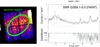 |
Fig. 15. An application of the mkacispback tool for the supernova remnant G359.1−0.5. Left panel: 0.7–5.0 keV image of the G359.1−0.5 region. The source region, which covers all the four ACIS-I CCDs, is shown with the green ellipse. Right panel: extracted spectrum and the output spectral model of mkacispback, as well as their residuals, are shown. The residuals below ∼7 keV are large because a model for the source emission has not been included here. |
4.3. Estimation of the unresolved intensity of the cosmic X-ray background
As a validation and application of mkacispback, here we evaluated the unresolved intensity of the cosmic X-ray background (CXB). Overall, we followed the analysis method adopted in Sects. 4 and 5 of Bartalucci et al. (2014) with an updated point source catalog in the CDF-S region by Luo et al. (2017). The data reduction was done as follows: cataloged point sources identified by Luo et al. (2017) were removed from individual CDF-S observations. The exclusion regions consist of circles with radii (r) depending on off-axis angle (θ) and source fluxes (f: photon flux in the 0.5–8.0 keV energy range). The r is defined as
![$$ \begin{aligned} r \,({\prime \prime }) = C_{\rm f} \,\left[ 1 + 10 \left( \frac{\theta \,({\prime \prime })}{600} \right) \right], \end{aligned} $$](/articles/aa/full_html/2021/11/aa41458-21/aa41458-21-eq5.gif)
where Cf is a scaling factor. The Cf is set to be 2, 4.5, 6, and 9 for f of f < 0.02 × 10⁻³ cnt s−1, 0.02 × 10⁻³ < f < 0.2 × 10⁻³ cnt s−1, 0.2 × 10⁻³ < f < 2 × 10⁻³ cnt s−1, and f > 2 × 10⁻³ cnt s−1, respectively. This exclusion was applied to the individual CDF-S observations listed in Table A.2. The analysis region is defined as a  square centered on RA(2000) =
  ,
,  . The spectrum was extracted from the analysis region for the entire CDF-S data set after the point-source exclusion.
To get the particle-induced background model suited for the analysis region, we ran mkacispback for each CDF-S observation and took an exposure-and-area-weighted sum of the model spectra. Following Bartalucci et al. (2014), the total spectral model to be compared to the observations was assumed to be

where Abs. is the Galactic absorption fixed to 8.8 × 1019 cm−2 (Stark et al. 1992) modeled with tbabs in XSPEC, and LP, HP, and CXBUR represent lower temperature (0.14 keV) and higher temperature (0.248 keV) thermal plasmas modeled with apec in XSPEC with solar abundances and the unresolved CXB modeled with powerlaw in XSPEC, respectively. The temperatures of the LP and HP models were fixed to the values obtained in Bartalucci et al. (2014), and only their normalizations were treated as free parameters. For the CXBUR model, the spectral index of 1.42 and a free normalization were assumed.
The analysis region is shown on the image, after point sources were removed, in the left panel of Fig. 16. We extracted spectra from the individual ACIS-I CCDs and performed a simultaneous spectral fit for them. In the spectral fit, we excluded two energy ranges near the line emission around 2.2 and 7.5 keV as there were significant residuals in these regions (see Sect. 4.1). Excluding these regions resulted in a better constraint on the normalization of the CXBUR component, which is the parameter of interest in this fit. The spectral fit is shown in the right panel of Fig. 16. The estimated unresolved CXB intensities (in erg s−1 cm−2 deg−2) are 3.10 (2.98–3.21)×10−12 in the 2–8 keV band, and 8.35 (8.00–8.70)×10−12 in the 1–2 keV band. These values are consistent with or lower than Hickox & Markevitch (2006), Bartalucci et al. (2014), and Luo et al. (2017)12.
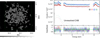 |
Fig. 16. Left panel: entire CDF-S image after point-source removal. Green square is the spectral extraction region. Right panel: represents the spectral fitting result. Data (crosses) and best-fit models (thick solid lines) are shown for four ACIS-I CCDs. Upper and lower panels: indicate the count rate and data-to-model ratio, respectively. The particle-induced background models are shown with thin solid lines. The unresolved CXB models are indicated with dashed lines. The 0.7–9.0 keV range was used for the spectral fit. Two energy ranges, 2.0–2.4 keV and 7.2–7.8 keV, were excluded from analysis. |
5. Conclusion
In this work, we investigated the particle-induced background properties of the Chandra ACIS-I and S1, S2, and S3 CCDs, and for both of the two data modes, FAINT and VFAINT. We used the ACIS-stowed and CDF-S blank-sky data sets to obtain spectral models to describe the background. We found and modeled the temporal variation of the spectral normalizations and shapes for the first time, as well as the spatial variations along the CHIPY axis by dividing each CCD into 32 regions in the CHIPY direction. The spectral hardness was found to vary in accordance with the total flux for the BI CCDs. Combining these temporal and spatial parameterizations, we developed a tool, mkacispback, to generate the particle-induced background spectrum for an arbitrary observation13. This tool was verified using the ACIS-stowed and CDF-S/CALDB blank-sky observations and was found to be reliable within 5% in the continuum and 8% around the lines. As a verification and application of our models, we also evaluated the unresolved CXB intensities as 3.10 (2.98–3.21)×10−12 erg s−1 cm−2 deg−2 in the 2–8 keV band, and 8.35 (8.00–8.70)×10−12 erg s−1 cm−2 deg−2 in the 1–2 keV band using mkacispback and the CDF-S observations. These estimates are consistent with or lower than previous ones.
Since cosmic-ray particles are decelerated by solar wind in the Solar System, the incoming cosmic-ray flux anti-correlates with solar activity (e.g. Mizuno et al. 2004).
This software is available at https://github.com/hiromasasuzuki/mkacispback.
For example, our estimates are lower than those of Bartalucci et al. (2014) by 10–20%. Such differences are probably due to the updated point-source catalog and slight difference in particle-induced background models.
Available at https://github.com/hiromasasuzuki/mkacispback.
All the base models including all the CCDs and data modes can be found on https://github.com/hiromasasuzuki/mkacispback.
Acknowledgments
We are grateful to the Chandra operation team and the IACHEC team for their patient operation, maintenance, and calibration of Chandra. We acknowledge the help by Catharine Grant in understanding the CHIPY-ΔE plots. H.S. appreciate the supports of the people at the Center for Astrophysics, Harvard-Smithsonian during my stay, which enabled this work. H.S. is supported by JSPS Research Fellowship for Young Scientists (Nos. 19J11069 and 21J00031) and Overseas Challenge Program for Young Researchers (No. 201980289). T.J.G. and P.P.P. acknowledge support under NASA contract NAS8-03060 with the Chandra X-ray Center.
References
- Arnaud, K. A. 1996, in Astronomical Data Analysis Software and Systems V, eds. G. H. Jacoby, & J. Barnes, ASP Conf. Ser., 101, 17 [NASA ADS] [Google Scholar]
- Bartalucci, I., Mazzotta, P., Bourdin, H., & Vikhlinin, A. 2014, A&A, 566, A25 [NASA ADS] [CrossRef] [EDP Sciences] [Google Scholar]
- Bearden, J. A., Burr, A. F., & States, U. 1967, in X-ray Wavelengths and X-ray Atomic Energy Levels [Electronic Resource], ed. J. A. Bearden (U.S. G.P.O Washington, D.C: U.S. Dept. of Commerce, National Bureau of Standards : For sale by the Supt. of Docs.), 66 [Google Scholar]
- Cash, W. 1979, ApJ, 228, 939 [Google Scholar]
- Fiandrini, E., Tomassetti, N., Bertucci, B., et al. 2021, Phys. Rev. D, 104, 023012 [NASA ADS] [CrossRef] [Google Scholar]
- Fruscione, A., McDowell, J. C., Allen, G. E., et al. 2006, in Observatory Operations: Strategies, Processes, and Systems, eds. D. R. Silva, & R. E. Doxsey, SPIE, 6270, 586 [Google Scholar]
- Gastaldello, F., Ghizzardi, S., Marelli, M., et al. 2017, Exp. Astron., 44, 321 [NASA ADS] [CrossRef] [Google Scholar]
- Grant, C. E., Miller, E. D., Bautz, M. W., et al. 2020. SPIE Conf. Ser., 11444, 1144442 [NASA ADS] [Google Scholar]
- Hagino, K., Odaka, H., Sato, G., et al. 2020, J. Astron. Telescopes Instrum. Syst., 6, 046003 [NASA ADS] [Google Scholar]
- Hickox, R. C., & Markevitch, M. 2006, ApJ, 645, 95 [NASA ADS] [CrossRef] [Google Scholar]
- Kaastra, J. S. 2017, A&A, 605, A51 [NASA ADS] [CrossRef] [EDP Sciences] [Google Scholar]
- Kuntz, K. D., & Snowden, S. L. 2008, A&A, 478, 575 [NASA ADS] [CrossRef] [EDP Sciences] [Google Scholar]
- Lotti, S., Mineo, T., Jacquey, C., et al. 2017, Exp. Astron., 44, 371 [NASA ADS] [CrossRef] [Google Scholar]
- Luo, B., Brandt, W. N., Xue, Y. Q., et al. 2017, ApJS, 228, 2 [Google Scholar]
- Marelli, M., Molendi, S., Rossetti, M., et al. 2021, ApJ, 908, 37 [CrossRef] [Google Scholar]
- Markevitch, M., Bautz, M. W., Biller, B., et al. 2003, ApJ, 583, 70 [Google Scholar]
- Mizuno, T., Kamae, T., Godfrey, G., et al. 2004, ApJ, 614, 1113 [NASA ADS] [CrossRef] [Google Scholar]
- NASA High Energy Astrophysics Science Archive Research Center (HEASARC) 2014, Astrophysics Source Code Library [record ascl:1408.004] [Google Scholar]
- Salvetti, D., Marelli, M., Gastaldello, F., et al. 2017, Exp. Astron., 44, 309 [Google Scholar]
- Stark, A. A., Gammie, C. F., Wilson, R. W., et al. 1992, ApJS, 79, 77 [Google Scholar]
- Suzuki, H., Bamba, A., Enokiya, R., et al. 2020, ApJ, 893, 147 [NASA ADS] [CrossRef] [Google Scholar]
- Tawa, N., Hayashida, K., Nagai, M., et al. 2008, PASJ, 60, S11 [NASA ADS] [Google Scholar]
- Wik, D. R., Hornstrup, A., Molendi, S., et al. 2014, ApJ, 792, 48 [NASA ADS] [CrossRef] [Google Scholar]
Appendix A: Logs of the ACIS-stowed and CDF-S blank-sky observations
ACIS-stowed observation logsa.
CDF-S blank-sky observation logs.a
Appendix B: Example of the base spectral models
An explicit spectral model for CHIPY = 993:1024 of I0 in VFAINT mode is presented here as an example.14 The entire XSPEC model is described as
gaussian + gaussian + gaussian + gaussian + gaussian + gaussian + gaussian + gaussian + gaussian + gaussian + gaussian + gaussian + gaussian + gaussian + gaussian + fsline + fsline + fsline + fsline + gabs*powerlaw + gabs*constant*expdec + gaussian.
The fsline is a user-defined model for the frame-store lines, which is described by Eq. 1. The model parameters are summarized in Table B.1. See Table 1 for the line identifications and Gaussian line energies in Table B.1. We note that the models to describe continuum are purely phenomenological and most of the parameters are physically meaningless.
Parameters of the analytical spectral model for CHIPY = 993:1024, I0, VFAINT mode.
Appendix C: Comparison between the individual ACIS-stowed observation spectra and output spectra of mkacispback
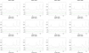 |
Fig. C.1. Comparison between the individual ACIS-stowed observation spectra and output spectra of mkacispback for ACIS-I0, VFAINT mode. In each case, the spectrum is extracted from the entire CCD. In each panel, the upper and lower panels show the data and model count rates (s−1 keV−1) and their ratios (data/model), respectively. One observation per year from the observation list (Table A.1) is presented. Observations with exposure time of less than 40 ksec are omitted. |
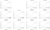 |
Fig. C.3. Same as Fig. C.1, but for ACIS-S1, VFAINT mode. No S1 data are available for OBSID 62678; for that observation, ACIS-I1 was on instead of ACIS-S1. |
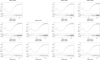 |
Fig. C.8. Same as Fig. C.1, but for ACIS-S1, FAINT mode. No S1 data are available for OBSID 62678; for that observation, ACIS-I1 was on instead of ACIS-S1. |
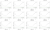 |
Fig. C.10. Same as Fig. C.1, but for ACIS-S3, FAINT mode. |
All Tables
Parameters of the analytical spectral model for CHIPY = 993:1024, I0, VFAINT mode.
All Figures
|
Fig. 1. Description of our analysis flow. The “stowed” and “blank-sky”, “merged” and “each obs.”, and “whole chip” and “32 slice regions” stand for the observation types, data types, and detector regions for which the analysis processes are applied, respectively. After the gain correction part, the “merged” and “each obs.” mean the gain-corrected-and-merged data and each of the gain-corrected observation data, respectively. A schematic drawing of a CCD chip with the 32 slice regions along CHIPY, readout direction, and frame-store region is also shown. |
| In the text | |
|
Fig. 2. Example spectrum of the observational particle-induced background extracted from a small region (CHIPX, CHIPY) = (1: 1024, 961: 992) of the I2 CCD. The data are extracted from the merged ACIS-stowed (black) and CDF-S blank-sky (red) observations. Upper and lower panels: present the fluxes and residuals, respectively. The data and the best-fit models are shown with the crosses and solid lines. The model components are presented with the dotted lines. We note that the spectral extraction region is far from the frame-store region so that the CTI effects are important. |
| In the text | |
|
Fig. 3. Gain slopes for individual ACIS-stowed observation data. The S1 data obtained in FAINT mode are excluded because the gain slopes are not determined well in this case due to less prominent line emissions. |
| In the text | |
|
Fig. 4. Gain slopes for individual CDF-S blank-sky observation data. |
| In the text | |
|
Fig. 5. Scatter plot of the particle-induced background events on the CHIPY-energy plane extracted from the merged ACIS-stowed data. This is the sum of the I0, I2, and I3 events. Darker regions include larger numbers of events. |
| In the text | |
|
Fig. 6. Scatter plots of events on the CHIPY-ΔE plane for I0 (CCD0), I2 (CCD2), and I3 (CCD3). The events were extracted from the gain-corrected-and-merged ACIS-stowed data in VFAINT mode. The extraction energy range is 9.628 ± 0.2 keV. The red solid lines represent the best-fit linear functions. |
| In the text | |
|
Fig. 7. Example of the spatial variation of the particle-induced background spectra. Two spectra extracted from the low- and high-CHIPY regions of the merged ACIS-stowed data (I0, VFAINT) are presented. Left panel: 32 slice regions along CHIPY. In each of the two right panels, the upper panel presents the data and model fluxes, whereas the lower panel presents their residuals. The black and red crosses represent the ACIS-stowed and CDF-S blank-sky observations, respectively. The solid and dotted lines are the total models and their components, respectively. |
| In the text | |
|
Fig. 8. Temporal variation of particle-induced background rate of ACIS-S3, FAINT mode. The transparent crosses are based on the rate of S3 events rejected onboard for exceeding the upper-level PHA threshold; they are scaled by ≈2% to be compared to the particle-induced background rate. The red and green ellipses enclose the observations at especially high and low particle-induced background rates. MJD stands for modified Julian date. |
| In the text | |
|
Fig. 9. Example of temporal variation of the particle-induced background spectral shapes. The black crosses represent the data. The black and red solid lines show the average spectral models and the models with the optimized hardness modification. We note that the OBSID 62850 and 62810 show the lowest and highest count rates in the ACIS-stowed observations, respectively. |
| In the text | |
|
Fig. 10. Hardness ratio (7.0–9.0 keV/1.0–7.0 keV) versus observation date. The black crosses and blue and red lines represent the data, average models, and models with the optimized hardness modification, respectively. The data and models are the ACIS-stowed observations processed in VFAINT mode. CCD 0, 2, 3, and 5–7 correspond to I0, I2, I3, and S1–S3, respectively. |
| In the text | |
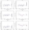 |
Fig. 11. Same as Fig. 10, but for the data processed in FAINT mode. |
| In the text | |
|
Fig. 12. Description of the process to generate the particle-induced background spectral model for arbitrary observation data, which are taken using the mkacispback tool. |
| In the text | |
|
Fig. 13. Merged observational spectra obtained in VFAINT mode and the output spectral models of mkacispback. The spectra were extracted from the entire CCD regions. The S1 and S3 data were taken from the CALDB blank-sky data instead of the CDF-S blank-sky data set. For each CCD, the upper and lower panels represent the count rate and data-to-model ratio, respectively. We note that the background was higher in the period covered by the CALDB blank-sky observations, so offsets between the ACIS-stowed and CALDB blank-sky data are present. |
| In the text | |
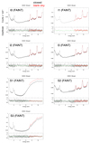 |
Fig. 14. Same as Fig. 13, but for the data processed in FAINT mode. |
| In the text | |
|
Fig. 15. An application of the mkacispback tool for the supernova remnant G359.1−0.5. Left panel: 0.7–5.0 keV image of the G359.1−0.5 region. The source region, which covers all the four ACIS-I CCDs, is shown with the green ellipse. Right panel: extracted spectrum and the output spectral model of mkacispback, as well as their residuals, are shown. The residuals below ∼7 keV are large because a model for the source emission has not been included here. |
| In the text | |
|
Fig. 16. Left panel: entire CDF-S image after point-source removal. Green square is the spectral extraction region. Right panel: represents the spectral fitting result. Data (crosses) and best-fit models (thick solid lines) are shown for four ACIS-I CCDs. Upper and lower panels: indicate the count rate and data-to-model ratio, respectively. The particle-induced background models are shown with thin solid lines. The unresolved CXB models are indicated with dashed lines. The 0.7–9.0 keV range was used for the spectral fit. Two energy ranges, 2.0–2.4 keV and 7.2–7.8 keV, were excluded from analysis. |
| In the text | |
|
Fig. C.1. Comparison between the individual ACIS-stowed observation spectra and output spectra of mkacispback for ACIS-I0, VFAINT mode. In each case, the spectrum is extracted from the entire CCD. In each panel, the upper and lower panels show the data and model count rates (s−1 keV−1) and their ratios (data/model), respectively. One observation per year from the observation list (Table A.1) is presented. Observations with exposure time of less than 40 ksec are omitted. |
| In the text | |
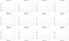 |
Fig. C.2. Same as Fig. C.1, but for ACIS-I3, VFAINT mode. |
| In the text | |
|
Fig. C.3. Same as Fig. C.1, but for ACIS-S1, VFAINT mode. No S1 data are available for OBSID 62678; for that observation, ACIS-I1 was on instead of ACIS-S1. |
| In the text | |
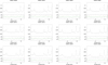 |
Fig. C.4. Same as Fig. C.1, but for ACIS-S2, VFAINT mode. |
| In the text | |
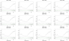 |
Fig. C.5. Same as Fig. C.1, but for ACIS-S3, VFAINT mode. |
| In the text | |
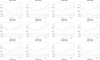 |
Fig. C.6. Same as Fig. C.1, but for ACIS-I0, FAINT mode. |
| In the text | |
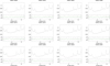 |
Fig. C.7. Same as Fig. C.1, but for ACIS-I3, FAINT mode. |
| In the text | |
|
Fig. C.8. Same as Fig. C.1, but for ACIS-S1, FAINT mode. No S1 data are available for OBSID 62678; for that observation, ACIS-I1 was on instead of ACIS-S1. |
| In the text | |
 |
Fig. C.9. Same as Fig. C.1, but for ACIS-S2, FAINT mode. |
| In the text | |
|
Fig. C.10. Same as Fig. C.1, but for ACIS-S3, FAINT mode. |
| In the text | |
Current usage metrics show cumulative count of Article Views (full-text article views including HTML views, PDF and ePub downloads, according to the available data) and Abstracts Views on Vision4Press platform.
Data correspond to usage on the plateform after 2015. The current usage metrics is available 48-96 hours after online publication and is updated daily on week days.
Initial download of the metrics may take a while.