| Issue |
A&A
Volume 655, November 2021
|
|
|---|---|---|
| Article Number | A90 | |
| Number of page(s) | 19 | |
| Section | Extragalactic astronomy | |
| DOI | https://doi.org/10.1051/0004-6361/202141244 | |
| Published online | 25 November 2021 | |
A low-energy explosion yields the underluminous Type IIP SN 2020cxd⋆
1
Department of Astronomy, The Oskar Klein Center, Stockholm University, AlbaNova, 10691 Stockholm, Sweden
e-mail: This email address is being protected from spambots. You need JavaScript enabled to view it.
2
Department of Particle Physics and Astrophysics, Weizmann Institute of Science, 234 Herzl St, 76100 Rehovot, Israel
3
Department of Physics, The Oskar Klein Center, Stockholm University, AlbaNova, 10691 Stockholm, Sweden
4
Division of Physics, Mathematics, and Astronomy, California Institute of Technology, Pasadena, CA 91125, USA
5
Astrophysics Research Institute, Liverpool John Moores University, IC2, Liverpool Science Park, 146 Brownlow Hill, Liverpool L3 5RF, UK
6
DIRAC Institute, Department of Astronomy, University of Washington, 3910 15th Avenue NE, Seattle, WA 98195, USA
7
IPAC, California Institute of Technology, 1200 E. California, Blvd, Pasadena, CA 91125, USA
8
Univ Lyon, Univ Claude Bernard Lyon 1, CNRS, IP2I Lyon / IN2P3, IMR 5822, 69622 Villeurbanne, France
9
Department of Astronomy, University of California, Berkeley, CA 94720-3411, USA
Received:
4
May
2021
Accepted:
17
August
2021
Abstract
Context. We present our observations and analysis of SN 2020cxd, a low-luminosity (LL), long-lived Type IIP supernova (SN). This object is a clear outlier in the magnitude-limited SN sample recently presented by the Zwicky Transient Facility’s (ZTF) Bright Transient Survey.
Aims. We demonstrate that SN 2020cxd is an additional member of the group of LL SNe and we discuss the rarity of LL SNe in the context of the ZTF survey. We consider how further studies of these faintest members of the core-collapse (CC) SN family might help improve the general understanding of the underlying initial mass function for stars that explode.
Methods. We used optical light curves (LCs) from the ZTF in the gri bands and several epochs of ultraviolet data from the Neil Gehrels Swift observatory as well as a sequence of optical spectra. We constructed the colour curves and a bolometric LC. Then we compared the evolution of the ejecta velocity and black-body temperature for LL SNe as well as for typical Type II SNe. Furthermore, we adopted a Monte Carlo code that fits semi-analytic models to the LC of SN 2020cxd, which allows for the estimation of the physical parameters. Using our late-time nebular spectra, we also make a comparison against SN II spectral synthesis models from the literature to constrain the progenitor properties of SN 2020cxd.
Results. The LCs of SN 2020cxd show a great similarity with those of LL SNe IIP in terms of luminosity, timescale, and colours. Also, the spectral evolution of SN 2020cxd is that of a Type IIP SN. The spectra show prominent and narrow P-Cygni lines, indicating low expansion velocities. This is one of the faintest LL SNe observed, with an absolute plateau magnitude of Mr = −14.5 mag and also one with the longest plateau lengths, with a duration of 118 days. Finally, the velocities measured from the nebular emission lines are among the lowest ever seen in a SN, with an intrinsic full width at half maximum value of 478 km s−1. The underluminous late-time exponential LC tail indicates that the mass of 56Ni ejected during the explosion is much smaller than the average of normal SNe IIP, we estimate M56Ni = 0.003 M⊙. The Monte Carlo fitting of the bolometric LC suggests that the progenitor of SN 2020cxd had a radius of R0 = 1.3 × 1013 cm, kinetic energy of Ekin = 4.3 × 1050 erg, and ejecta mass of Mej = 9.5 M⊙. From the bolometric LC, we estimated the total radiated energy Erad = 1.52 × 1048 erg. Using our late-time nebular spectra, we compared these results against SN II spectral synthesis models to constrain the progenitor zero-age main sequence mass and found that it is likely to be ≲15 M⊙.
Conclusions. SN 2020cxd is a LL Type IIP SN. The inferred progenitor parameters and the features observed in the nebular spectrum favour a low-energy, Ni-poor, iron CC SN from a low-mass (∼12 M⊙) red supergiant.
Key words: supernovae: general / galaxies: individual: NGC 6395
Photometry is only available at the CDS via anonymous ftp to cdsarc.u-strasbg.fr (130.79.128.5) or via http://cdsarc.u-strasbg.fr/viz-bin/cat/J/A+A/655/A90
© ESO 2021
1. Introduction
Stars that are more massive than about 8 M⊙ end their lives with the collapse of their iron core. Type II supernovae (SNe) are the most common among these core-collapse (CC) explosions and they are characterised by the presence of hydrogen in their spectra. Type II SNe constitute a diverse class, with light curves (LCs) showing different decline rates across a continuum and a broad range of luminosities, with V-band maximum absolute magnitudes ranging from about −13.5 to −19 mag (Anderson et al. 2014).
Low-luminosity SNe II (LL SNe II) make up a small part on the faint tail of the detected Type II SN distribution. There are only a dozen such objects presented in the literature (see Table 1), including three recently published examples (Jäger et al. 2020; Müller-Bravo et al. 2020; Reguitti et al. 2021). These are SNe with a faint plateau (SNe IIP) and a late LC tail signalling radioactive powering by a small amount of ejected 56Ni, typically ∼0.005 M⊙ (Spiro et al. 2014, their Fig. 13). LL SNe II often also display slow expansion velocities, suggesting low explosion energies.
Properties of the sample of LL SNe IIP.
It has now been well established that the progenitors of many SNe II are red supergiant (RSG) stars (Smartt et al. 2009) and it is suspected that the LL SNe IIP originate from stars with relatively low zero-age main sequence (ZAMS) masses (∼8–10 M⊙, Pumo et al. 2016; O’Neill et al. 2021). However, other studies have suggested the possibility that the progenitors are more massive RSGs with large amounts of fallback material (Zampieri et al. 2003) or electron capture supernova (ECSN) explosions of super-asymptotic giant branch (SAGB) stars (Hiramatsu et al. 2021). There are several methods available for deriving information about the exploded star, including the identification of SN progenitors in archive images (e.g., Smartt et al. 2009), light curve modelling (e.g., Arnett & Fu 1989), and late-time nebular spectral modelling (e.g., Jerkstrand et al. 2012, 2018; Dessart et al. 2013; Lisakov et al. 2016).
For a typical initial mass function (IMF), over 40% of the potential CC SN progenitors reside in the 8 − 12 M⊙ range and 25% in the 8 − 10 M⊙ range (Sukhbold et al. 2016). The fact that the LL SNe are rarely detected and underexplored is, of course, due to the many observational biases challenging the discovery and follow-up of such faint transients. Most of them have been discovered in targeted searches of relatively nearby galaxies. However, with the ongoing revolution in transient science, with systematic non-targeted surveys uncovering thousands of transients, this is beginning to change. In this paper, we use data from one of the ongoing surveys, the Zwicky Transient Facility (ZTF; Bellm et al. 2019; Graham et al. 2019). In particular, Fremling et al. (2020) introduced the ZTF Bright Transient Survey (BTS), which provides a large and purely magnitude-limited sample of extragalactic transients in the northern sky that is suitable for a detailed statistical and demographic analysis. Perley et al. (2020a) presented early results of the BTS, which is almost spectroscopically complete down to a target magnitude of 18.5. In particular, they presented a CC SN luminosity function, in which a significant fraction of the CC SNe is very dim. They state that this is in agreement with works arguing that the ‘SN rate problem’ (Horiuchi et al. 2011) can be resolved using galaxy-untargeted surveys and including the faint end of the SN luminosity function.
Similar efforts to construct an unbiased view of the Type II SN luminosity function comes from the parallel ZTF volume-limited survey, the ZTF Census of the Local Universe (CLU) experiment, which extends the classification threshold to m ≲ 20 mag for transients occurring in known galaxies within D < 200 Mpc (De et al. 2020). These results also suggest that the lowest luminosity events are more common than previously appreciated (Tzanidakis et al., in prep.). The ultimate aim of such extensive efforts is to be able to connect SN rates with star-formation rates and to couple the stellar evolution IMF to the known SN populations.
Out of the 171 Type II SNe presented by Perley et al. (2020a), one object clearly stands out as being both longer in duration and considerably fainter than the rest of the population, SN 2020cxd (a.k.a. ZTF20aapchqy, Perley et al. 2020a, their Fig. 7). The authors have asserted that this is ‘almost certainly the explosion of a massive star’. In this paper, we take the opportunity to present SN 2020cxd in greater detail. We argue that this transient is not only interesting in its aspect as a single object, given the rarity of LL SNe in the literature, but that this event is important in the context of the overall population of SNe II provided by the strict and clear criteria of the highly complete BTS sample.
This paper is structured as follows. In Sect. 2, we outline the observations and corresponding data reductions; in particular, Sect. 2.1 presents the discovery and classification of SN 2020cxd. The ground-based optical SN imaging observations and data reductions are presented in Sects. 2.2 and 2.3, we describe the Swift observations. We present our search for pre-explosion outbursts in Sect. 2.4, with the optical spectroscopic follow-up campaign described in Sect. 2.5 and a discussion of the host galaxy provided in Sect. 2.6. Our analysis and a discussion of the results is given in Sect. 3 and we provide a summary in Sect. 4. Some of the more technical aspects of the analysis are presented in the appendix.
2. Observations and data reduction
2.1. Discovery and classification
SN 2020cxd was first discovered with the Palomar Schmidt 48-inch (P48) Samuel Oschin telescope on 19 February 2020 (JDdiscovery = 2458899.0306), as part of the ZTF survey. The first ZTF detection was made in the r band, with a host-subtracted magnitude of 17.69 ± 0.05 mag, at the J2000 coordinates α = 17h26m29.26s, δ = +71 ° 05′38.6″. The first g-band detection came in 31 min later, at 17.63 ± 0.04. An on-duty astronomer (JS) immediately triggered follow-up observations and several telescopes started observing shortly thereafter. The discovery was reported to the Transient Name Server (TNS1) by Nordin et al. (2020), with a note that the last non-detection was three days earlier on February 16, with a global limit of 20.4 in the g band. We can therefore constrain the epoch of explosion for this SN with a good level of precision. In this paper, we adopt an explosion date of JDexplosion = 2 458 897.5301, with an uncertainty of ±1.5 days, as given by the epoch halfway between discovery and last non-detection2.
SN 2020cxd is positioned in the nearby spiral galaxy NGC 6395, which has a measured redshift of z = 0.003883. According to the NASA/IPAC Extragalactic Database (NED)3 catalog, the peculiar motion corrected distance for a standard cosmology (ΩM = 0.3, ΩΛ = 0.7, and h = 0.7) is 23 Mpc, whereas the most recent Tully–Fisher measurement reported on the same site is 20 Mpc. In this paper, we adopt a distance modulus of 31.7 ± 0.3 mag (22 ± 3 Mpc). We also obtain the amount of Galactic extinction along the line of sight using the NED extinction tool4 (based on the dust map of Schlafly & Finkbeiner 2011) and adopt E(B − V) = 0.035 mag. The SN together with the host galaxy and the field of view is shown in Fig. 1.
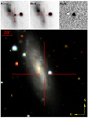 |
Fig. 1. SN 2020cxd in the nearby galaxy NGC 6395. The g-band image subtraction is shown in the top panels (subtraction to the right), with the SN image observed on 24 April 2020 – 64.9 days after the first ZTF detection (to the left). Bottom panel: a gri-colour composite image of the host galaxy and its environment. It was composed of ZTF g-, r- and i-band pre-explosion images of the field. |
SN 2020cxd was classified as a Type II SN (Perley et al. 2020b; Perley 2020) based on a spectrum obtained on 20 February 2020, at 17 h past discovery, with the Liverpool telescope (LT) equipped with the SPectrograph for the Rapid Acquisition of Transients (SPRAT). That spectrum revealed a blue continuum with hydrogen P-Cygni features (broad Hα and Hβ). The classification was consolidated with a spectrum taken four hours thereafter, with the Palomar 60-inch telescope (P60; Cenko et al. 2006) equipped with the Spectral Energy Distribution Machine (SEDM; Blagorodnova et al. 2018).
2.2. Optical photometry
Following the discovery, we obtained regular follow-up photometry during the 100+ day plateau phase in the g, r, and i bands with the ZTF camera (Dekany et al. 2020) on the P48. Early LT photometry in ugriz was also obtained at one epoch to measure the colours and a campaign with the Swift observatory was launched (Sect. 2.3). Later on, after the drop from the plateau, we also obtained a few epochs of photometry in gri with the SEDM on the P60, with the LT telescope and with the Nordic Optical telescope (NOT), using the Alhambra Faint Object Spectrograph (ALFOSC). The photometric magnitudes of SN 2020cxd are listed in Table 2.
Summary of ground-based photometry for SN 2020cxd.
The LCs from the P48 come from the ZTF pipeline (Masci et al. 2019). Photometry from the P60 were produced with the image-subtraction pipeline described in Fremling et al. (2016), with template images from the Sloan Digital Sky Survey (SDSS; Ahn et al. 2014). This pipeline produces point spread function (PSF) magnitudes, calibrated against SDSS stars in the field. For the late NOT images, template subtraction was performed with hotpants5, using archival SDSS images. The magnitudes of the transient were then measured using SNOoPY6 and calibrated against SDSS stars in the field. All magnitudes are reported in the AB system. The reddening corrections are applied using the Cardelli et al. (1989) extinction law with RV = 3.1. We do not correct for host galaxy extinction, since there is no sign of narrow NaI D absorption lines in our spectra. This is basically an assumption and we discuss some of the implications of this towards the end of the paper. The gri LCs are shown in Fig. 2.
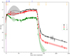 |
Fig. 2. Light curves of SN 2020cxd in the g (green symbols), r (red), and i (black) bands. These are host-subtracted magnitudes from the P48, P60, and LT, as well as two epochs from the NOT on the late tail. Forced photometry obtained using SNOoPY is plotted as open circles. All are observed (AB) magnitudes in the observer frame in days since the explosion. Relevant upper limits are displayed as inverted triangles, and constrain the explosion epoch of the SN (the purple vertical dashed line), as well as the g-band tail. The dashed lines with error regions are Gaussian process estimates of the interpolated and extrapolated LC. After 150 days, we show the linear fits instead. The yellow downward pointing arrows on top indicate the epochs of spectroscopy, the blue vertical bars display the epochs with Swift observations. |
We used a Gaussian process (GP) algorithm7 to interpolate the photometric measurements and found8 that the peak happened at  after
after  rest frame days past explosion. In the i band, the photometric behavior followed the same trend and reached a maximum at
  after
after  rest frame days. The g-band light curve actually peaks at the first detection epoch. It slowly declines before it flattens out on a plateau, which reaches a maximum at mg = 18.08 after 115.26 days. Thereafter, the SN declined fast and soon became too faint for detection with the P48. We then activated the LT and NOT telescopes. The r- and i-band observations on the tail suggest a linear decline. We performed a linear fit after ∼150 days, and found that the best fit slopes for the r and i band are (8.86 ± 1.33)×10−3 and (9.99 ± 0.79)×10−3 mag days−1, which are consistent with the radioactive cobalt decay slope (λCo = 1/111.3 × 2.5/ln(10)∼9.76 × 10−3 mag days−1). For the g-band images on the tail, we found no apparent flux in the LT and NOT residual images down to 2.5 sigma (upper limits are also presented in Table 2).
2.3. Swift-observations: UVOT photometry
A series of ultraviolet (UV) and optical photometry observations were obtained with the UV/Optical Telescope onboard the Neil GehrelsSwift observatory (UVOT; Gehrels et al. 2004; Roming et al. 2005) between 20 February and 2 June 2020. Our first Swift/UVOT observation was performed on 20 February 2020 (JD = 2 458 899.8624), at 0.83 days past discovery (2.3 days past estimated explosion). The SN was detected in all bands. The brightness in the UVOT filters was measured with UVOT-specific tools in HEAsoft9.
Source counts were extracted from the images using a circular region with a radius of 3″. The background was estimated using a circular region with a radius of 39″. The count rates were obtained from the images using the Swift tool uvotsource and converted to magnitudes using the UVOT photometric zero points (Breeveld et al. 2011) and the new calibration data from September 202010. We obtained a final UVOT epoch in August 2020, after the SN had faded, to remove the host contribution from the transient light curve. A log of the Swift observations is provided in Table 3. This includes six epochs in total, and these epochs are also indicated in Fig. 2. Such a dense and early UV coverage is very rare for LL SNe, and is important for constructing the bolometric light curve needed to model the SN in Sect. 3.3; see also Appendix A.
Summary of Swift observations for SN 2020cxd.
2.4. Pre-discovery imaging
Since the SN occurred in a very nearby galaxy, we decided to search for pre-explosion activity of the progenitor star. For this purpose, we downloaded IPAC difference images11, performed forced photometry at the SN position (Yao et al. 2019), applied quality cuts, and searched for pre-explosion detections, as described by Strotjohann et al. (2021).
The ZTF started to monitor the position of SN 2020cxd 2.5 years before the discovery and we searched for pre-explosion outbursts in 999 observations collected on 307 different nights that were obtained in the g, r, and i bands. No outbursts are detected above the 5σ threshold when searching unbinned or binned (1–90-day long bins) LCs. Figure 3 shows the absolute magnitude LC in seven-day bins, where filled data points are significant at the 5σ level while arrows indicate 5σ upper limits. The g-band (r-band) observations are available in 69 (68) out of 132 weeks before the SN discovery and we can exclude flares brighter than an absolute magnitude of −10 in 46 weeks (41 weeks), that is, 34% (31%) of the time.
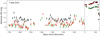 |
Fig. 3. ZTF P48 pre-explosion images for SN 2020cxd reveal no precursors in g (green symbols), r (red), or i (black) bands. Filled data points are ≳ 5σ detections, whereas arrows show 5σ upper limits. The data are binned in seven-day bins. |
2.5. Optical spectroscopy
A spectroscopic follow-up was conducted with SEDM mounted on the P60 and with the LT SPRAT spectrograph on La Palma. Further spectra were obtained with the NOT using ALFOSC as well as one epoch with Gemini North and GMOS and a final spectrum with Keck and LRIS. A log of the nine obtained spectra is provided in Table 4. The SEDM spectra were reduced using the pipeline described by Rigault et al. (2019), and the LT and NOT spectra were reduced using standard pipelines. The spectra were finally absolute-calibrated against the r-band photometry using the GP interpolated magnitudes and then corrected for Milky Way (MW) extinction. All spectral data and corresponding information is made available via WISeREP12 (Yaron & Gal-Yam 2012). We present the sequence of spectra in Fig. 4, while the epochs of spectroscopy are also highlighted in Fig. 2. Overall, we managed to acquire spectra over the full relevant range of the SN evolution, but it should also be noted that the photospheric part of the evolution is mainly covered by robotic telescopes providing limited resolution and signal.
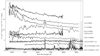 |
Fig. 4. Sequence of optical spectra for SN 2020cxd, corrected for redshift and reddening. The complete log of spectra is provided in Table 4. The epoch (rest frame days since explosion) of the spectra is provided to the right. The spectra are shifted in flux by a constant for clarity. Late time spectra are scaled for comparison. The scaling factors are also listed to the right. Some spectra are also binned (shown as black lines), with a window size of 5 Å for LT, and 10 Å for NOT/Gemini/Keck, and their original spectra are shown in shaded grey. |
Summary of spectroscopic observations for SN 2020cxd.
2.6. Host galaxy
NGC 6395 is a nearby grand Scd spiral galaxy in the Draco constellation, which has not been reported to host any SN before. Simbad reports an AB magnitude of 13 in the r band, but there is no SDSS spectrum of this galaxy and we have not been able to find any estimates of the metallicity of NGC 6395. We therefore made use of some of the spectroscopic observations of the SN to also measure some of the stronger emission lines from the nearby regions as a way to probe the metallicity of the gas close to the site of the explosion. The late Keck spectrum was taken with the slit oriented through the galaxy, and we extract the spectrum of an H II region located 8″ north of the SN to probe the gas-phase metallicity there. We discuss our results in Sect. 3.4.
3. Analysis and discussion
3.1. Light curves
The g-, r-, and i-band LCs of our SN are displayed in Fig. 2. In the figure, we have also included the most restrictive upper limits as triangles (2.5σ), while the arrows on top of the figure illustrate epochs of spectroscopy. The GP interpolation (at early phases) and linear fits (during nebular phases) are also shown.
It is clear that SN 2020cxd must have risen very swiftly in the first few days. The rise is 2.57 magnitudes (r band) in three days or less, with the slope thus larger than 0.85 mag per day. This fast rise of SN 2020cxd is comparable to that of the LL SN 2005cs (0.90 mag day−1 in the R band, see Fig. 5 and Pastorello et al. 2009, their Fig. 4).
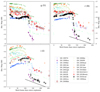 |
Fig. 5. Absolute magnitudes of SN 2020cxd (black stars) together with the LCs of other LL SNe IIP, as well as for the normal Type II SN 1999em (green circles). We highlight SN 2013am (orange circles) which is the brightest within the LL SN II sample, and SNe 1999eu (purple circles) and 1999br (blue circles) which are the faintest. We also use a larger marker for SN 2018hwm (red hexagons), which was also monitored by ZTF in gri photometry. The other SNe are displayed with smaller and fainter markers. The LCs are plotted versus rest frame days past explosion. The radioactive cobalt decay rate is shown as a black line in the r- and i-band panels for comparison. The photometric data were obtained via the Open Supernova Catalog. Data reference for SN 1999em is Leonard et al. (2002), and for the LL SNe II these are listed in Table 1. |
After that initial rise follows a plateau phase of 100+ days, which firmly establishes SN 2020cxd as a Type IIP SN. The plateau is, however, not completely flat. In the g band, there is an initial decline, which levels off and then very slightly rises until the end of this phase. The r-band LC shows an initial undulation, but is then slowly rising by about 0.5 mag in 100 days, and the i band is following in that rise. The LC is well sampled with 58 observations (r band) over the plateau that allow us to discern such unusual LC structures.
The drop from the plateau is sharp and fast. The g-band LC declines by 4.98 mag in only 28 days. The drop in the r and i bands are slightly shallower, making SN 2020cxd redder at the very late-time phases, but the more optimally sampled r-band LC also sharply plummets by 1.9 mag in only six days.
When making a comparison with the large compilation of Type II LCs from Anderson et al. (2014) and using their nomenclature13, we find that the optically thick phase duration (OPTd) of SN 2020cxd is 118.3 ± 3.0 d14, which is one of the longest plateau lengths compared to the Anderson sample, and the decline rate during plateau phase (s2) is −0.73 mag per 100 days, which is also very rare15. Most of the SNe IIP have instead a clearly positive s2 slope, that is, the plateau is slowly declining in luminosity, and SN 2020cxd is thus an unusually well-sampled example of a brightening plateau.
In Fig. 5, we show the r/R-, g/V- and i/I-band LCs in absolute magnitudes together with the LCs of several other LL SNe II (see Table 1 for detailed information). Since most of the LL SNe II in the literature were observed in the Johnson photometric system, we compare LCs between r/R, g/V, and i/I, correspondingly. They show similarity with the canonical Type II plateau SN 1999em (green circles). The magnitudes in Fig. 5 are in the AB system16 and have been corrected for distance modulus, MW extinction, and host extinction if any, and are plotted versus rest frame days past estimated explosion epoch (see Table 1).
The figure demonstrates that SN 2020cxd is a clear member of this population of LL SNe and in many respects it represents a rather typical representative example for this class. The improved photometric sampling compared to most other objects allows us to clearly see the on-plateau evolution. The well-determined explosion epoch and the sharp drop from the plateau also allows for a more precise measure of the plateau duration (OPTd).
The colour evolution of SN 2020cxd and the other LL SNe is shown in Fig. 6. We plot (g − r)/(V − R) in the upper panel and (r − i)/(R − I) in the lower panel, both corrected for MW extinction. In doing so, no interpolation was used. Given the excellent LC sampling we used only data where the pass-band magnitudes were closer in time than 0.1 days. A comparison is made with the colour evolution for other LL SNe, which are known to typically be redder than ordinary SNe II. Compared to this sample, our SN is similar, which implies that the amount of additional host extinction is indeed likely small compared to the rest of this population, in accordance with our assumption of negligible host extinction. Our SN shows normal g − r colours at early phases, and evolves towards the redder part of the sample population after about a month. The r − i stays in the lower part of the LL SN II colour space over the entire plateau phase.
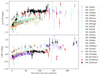 |
Fig. 6. Colour evolution of SN 2020cxd (black stars) shown in g − r (upper panel) and r − i (lower panel). The colours have been corrected for MW extinction. For comparison, we have also plotted colours for several other LL SNe II. Most of these are V − R and R − I. For references see Table 1. |
3.2. Spectra
The log of the spectroscopic observations is provided in Table 4 and the sequence of spectra is shown in Fig. 4. Overall, the spectra of SN 2020cxd are typical for a Type II SN. In this section, we compare the spectra of SN 2020cxd with spectra from other LL Type IIP SNe at different phases.
Spectral comparisons between SN 2020cxd and other LL SNe IIP at photospheric phases are provided in Fig. 7. All spectra have been corrected for redshift and galactic reddening. Within ∼10 days after explosion, all of the comparison SNe show very blue continuum, with dominant line features of Balmer lines and Na I D17.
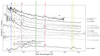 |
Fig. 7. Sequence of early photospheric spectra for SN 2020cxd, compared with spectra of other LL Type IIP SNe in grey. The epoch of the spectrum is provided to the right. Some identified lines (H, Na I D and Ca NIR triplet) are marked as vertical dashed lines. We also mark several metal lines as short vertical lines, which might be present in the last P60 spectrum. |
As SN 2020cxd enters the plateau phase, the spectrum becomes redder as the photospheric temperature decreases. At +93 days, the Ca II near-infrared (NIR) triplet of SN 2020cxd is well developed, and we can also discern several metal lines, for instance: Fe II, Sc II, and Ba II (Fig. 7).
From ∼120 days onwards, SN 2020cxd enters the optically thin phase and the luminosity decreases rapidly. The spectra displayed in Fig. 4 are all absolute calibrated against r-band photometry as interpolated from the LC, and the last three nebular spectra have been scaled by factors of 2, 10, and 15, respectively, for an easier comparison. Figure 8 shows the scaled late-time spectra compared to other LL SNe II at similar phases. From 160 days, the spectra are dominated by Hα, [Ca II] λλ7291, 7323, and the Ca II NIR triplet.
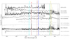 |
Fig. 8. Sequence of nebular spectra for SN 2020cxd, compared with spectra of other LL Type IIP SNe in grey. The epoch of the spectrum is provided to the right. Some identified lines, e.g., Hα, [Ca II] λλ7291, 7323, Ca II NIR triplet, [O I] λλ6300, 6364, and λ8446, are marked as vertical dashed lines. |
During the photospheric phase, we measured the velocities for SN 2020cxd using iraf18 to make a Gaussian fit to the minimum of the absorption lines of the corresponding P-Cygni profiles. Velocities and their uncertainties were estimated by a random sampling on the Gaussian fits to the minimum, by shifting the anchor continuum points a 1000 times within a region of ±5 Å, using astropy.modeling.Gaussian1D for the iteration. Fits with bad chi-squared values were excluded.
The difference between the minimum of the best-fit Gaussian and the line location was translated to an expansion velocity. In the late nebular phase, we instead estimated the velocities from the emission line full width at half maximum (FWHM), which is the width measured at half level between the continuum and the peak of the line, and corrected for the instrumental resolutions obtained from the sky lines. These velocities are displayed in Fig. 9, where we also make a comparison with other LL Type IIP SNe. The velocities for the comparison sample are taken from Pastorello et al. (2004) to Spiro et al. (2014). The time evolution of the velocities measured for Hα matches well with those of other LL Type IIP SNe at similar epochs, but also extend to earlier phases. The velocities of all these LL SNe, including SN 2020cxd, are very low, clearly lower than for the normal Type IIP SN 1999em. We notice that the Hα velocity of SN 2020cxd became very low around 250 days after the explosion, that is, we measured an intrinsic FWHM of 478 km s−1, in the last Keck spectrum (Fig. 8). This is among the narrowest lines ever measured for a SN IIP.
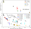 |
Fig. 9. Velocity evolution of SN 2020cxd. Upper panel shows the expansion velocities estimated from Hα P-Cygni minima (black stars) and FWHM (red stars), Hβ P-Cygni minima (yellow squares), [Ca II] λ7291 line FWHM (blue cross), FWHM of Ca II NIR triplet middle line (green diamonds), and [O I] λ6300 line FWHM (orange pentagons). Hα velocities for SN 2020cxd compared to other LL SNe discussed throughout the paper. A comparison with the normal Type II SN 1999em is shown in the lower panel. The x-axis shows the phase with respect to explosion. Line velocities of the other LL SNe II are taken from Pastorello et al. (2004) to Spiro et al. (2014). |
An important method for diagnosing the progenitor mass is through late-time spectral modelling. At the optically thin phase we are observing deeper into the progenitor structure (Jerkstrand et al. 2012). Figure 10 shows our last Keck spectrum taken during the optically thin phase, compared to the modelling. The Keck spectrum is absolute calibrated against r-band interpolated photometry. In order to estimate the progenitor mass of SN 2020cxd, we collected spectral synthesis models of SNe II (with 12, 15, and 19 M⊙ ZAMS masses) from the literature (Lisakov et al. 2016; Jerkstrand et al. 2012, 2014; Dessart et al. 2013). The models were selected based on their having similar phases to the SN observation they are are shifted to the distance of SN 2020cxd, as well as scaled by the nickel mass. As discussed, for instance, in Jerkstrand et al. (2014) and Müller-Bravo et al. (2020), the luminosity of some lines, like [O I] λ6300, 6364, scales relatively linearly with the ejected nickel mass, thus, it is reasonable to scale the model fluxes by nickel mass for the comparison. To fit the models to the data, we implement a simple Monte Carlo approach that randomly scales the models, while the χ2 values were calculated to quantify the comparisons19. In Fig. 10, the five theoretical models with best fit scaling factors are compared to the Keck spectrum of SN 2020cxd at ∼240 d. As shown, the 19 M⊙ model at this phase is dominated by Hα and under-predict the observed fluxes of the other elements. For the four less massive progenitor models, we see that the models partially reproduce the [O I] λ6300 line. The Jerkstrand 12 and 15 M⊙ models under-predict the [O I] λ6364 by 40%. The Dessart 15 M⊙ model reproduces the [Fe II] λ7155 of SN 2020cxd well, while for the rest of the spectrum, the differences are relatively larger (by ∼30–40%). The Jerkstrand models do not reproduce the Ca II NIR triplet, while the Lisakov 12 M⊙ model does a good job reproducing it, better than in the Dessart 15 M⊙ model. The Lisakov model over-predict the [Ca II] λλ7291, 7323 by a factor of 2, whereas the other models agree better. In terms of χ2 values, the scaled Dessart 15 M⊙ model gives the best match, slightly better than the other three models. Overall, we conclude that the progenitor of SN 2020cxd had a ZAMS mass less than 19 M⊙. However, to properly distinguish between 12 M⊙ and 15 M⊙ models, a more detailed comparison is needed. We note that for lower-mass progenitors, a smaller line ratio of [O I]/[Ca II] is also expected due to the lower O-core mass (Maeda et al. 2007; Jerkstrand et al. 2012; Fang & Maeda 2018). Using our absolute calibrated Keck spectrum, we measured the fluxes for [O I] λλ6300, 6364, and [Ca II] λλ7291, 7323, and estimated a ratio of 0.82, which favours a lower mass progenitor.
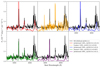 |
Fig. 10. Comparison between the last Keck spectrum of SN 2020cxd at nebular phases and scaled synthetic spectra. The black curves are the observed spectra, binned with a window size of 10 Å, and corrected for redshift and extinction. The models are displayed with coloured lines, and originate from Jerkstrand et al. (2012, 2014), Dessart et al. (2013), Lisakov et al. (2016). These were obtained via WISeREP. The models are scaled by nickel mass ratio. All model spectra are shifted to the SN distance by the inverse square of the distance. Their rest frame phases and scaling factors are shown in the legend. |
3.3. Bolometric light curve
In order to estimate the total radiative output, we attempted to construct a bolometric LC. We performed a blackbody (BB) fitting every two days with the GP interpolated gri data of SN 2020cxd during its photospheric phase, that is, up to ∼120 rest frame days. More details about the diluted BB fitting and the UV/IR contributions to the bolometric LC are discussed in Appendix A.
At nebular phases, the BB fits are not applicable and we use the bolometric correction (BC) approach to estimate the bolometric magnitudes of SN 2020cxd. In this work, we use the BC of SN 2018hwm to estimate the bolometric LC of SN 2020cxd. More information on this approach is provided in Appendix B.
The best-fit bolometric luminosity LC of SN 2020cxd is thus composed of the early part from BB fitting and the tail, inferred using the BC, and is shown as red stars in Fig. 11, compared to other LL Type IIP SNe discussed throughout the paper. As shown, SN 2020cxd is similar to the other LL SNe II, which are fainter than the famous SN 1987A. The slope of the LC tail matches well with the Cobalt decay rate.
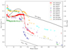 |
Fig. 11. Bolometric luminosities of several LL SNe IIP and the famous SN 1987A. The luminosity of SN 2020cxd (shown as the red stars) was calculated after accounting for MW extinction and distance. The slope of the luminosity tail matches well with the radioactive decay of 56Co. |
We can now calculate the bolometric peak luminosity of SN 2020cxd, which is  erg s−1 at 103 rest frame days and a total radiated energy over the first 200 rest frame days of Erad = 1.52 × 1048 erg.
From the BB approximation, we also obtained the temperature and the evolution of the BB radius. The obtained temperatures and radii are compared to those of other LL SNe in Fig. 12. SN 2020cxd follows a similar evolution in these parameters as the other LL SNe II in this sample, with both temperature and radius at the lower bound of the distribution. This is sensitive to the amount of host extinction and allowing for additional extinction would increase the temperature.
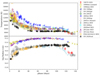 |
Fig. 12. Temperature and radius of several LL SNe IIP, including SN 2020cxd (shown as black stars). Upper panel: evolution of their photospheric temperature estimated by fitting a blackbody to the SED in the optically thick phase. Bottom panel: evolution of their photospheric radius based on the same fits. We followed Jäger et al. (2020) in the methodology and the included SNe are also from that paper. |
The ejected 56Ni mass can be inferred by measuring the luminosity tail, which is powered by the decay of radioactive elements, namely, 56Co, synthesised in the explosion. Using, L = 1.45 × 1043 exp erg s−1 from Nadyozhin (2003) implies that we would require 0.002 ± 0.001 M⊙ of 56Ni to account for the tail luminosity (> 140 days). We note that the uncertainty in distance modulus affects this estimate with a systematic uncertainty of ≲30%, but an additional host extinction of E(B − V)host = 0.25 mag would increase this by a factor of two.
In order to estimate progenitor and explosion parameters from the photometry, we make use of a Markov chain Monte Carlo (MCMC) code recently presented by Jäger et al. (2020), which fits semi-analytic models to quasi-bolometric LCs (see Appendix C for more details). We employed the MCMC to fit the semi-analytic models to SN 2020cxd, the acceptable fits are displayed as light solid black lines in Fig. C.1. After marginalisation, we obtained estimates with confidence intervals (1σ) for each of these parameters, namely: SN 2020cxd has  cm (∼187 R⊙),
  M⊙,
M⊙,  erg,
erg,  km s−1,
  erg, for its progenitor radius, ejecta mass, kinetic energy, expansion velocity, and thermal energy, respectively. The nickel mass was simultaneously estimated as 0.003 ± 0.002 M⊙.
Reguitti et al. (2021) estimated the ejected mass of SN 2018hwm to 8 M⊙. By assuming the mass of the compact remnant and a typical mass loss during the pre-SN stage, they estimated that the initial progenitor mass (ZAMS mass) of SN 2018hwm was in the range of 9.4 − 10.9 M⊙. For SN 2020cxd, the ejected mass is estimated to be ∼9.5 M⊙. With the same assumptions, its ZAMS mass was then between 10 and 14 M⊙.
The initial bolometric decline (first 20 days) somewhat mimics those suggested to be powered by CSM in some hydrodynamical models (Morozova et al. 2017), but no evidence was found for flash spectroscopy features (e.g., Bruch et al. 2021) in our very early spectra (< 3 days past explosion). Overall, there is no evidence for CSM interaction from narrow spectral lines, UV brightness or from the shape of the LC. These consideration could disfavour a SAGB star as a potential progenitor star, since these are thought to have high mass-loss rates (compared to those of RSG stars of a similar initial mass, Hiramatsu et al. 2021).
There have been extensive studies carried out on the duration of the LC plateau for Type II SNe in the literature, exploring, for example, the effect of radioactivity on this phase. Although it has been well established that the luminosity in this period derives from the diffusion as the photosphere recedes, it has also been suggested that the duration of the plateau is affected by radioactive input (Popov 1993; Kasen & Woosley 2009; Nakar et al. 2016). The most important parameter for the plateau duration in the investigation of Pumo et al. (2016) was the amount of stripping of the ejecta, where extensive stripping led to shorter plateau lengths. In this context, the very long duration in SN 2020cxd might suggest that the ejecta must have remained relatively intact. Kasen & Woosley (2009) derived scaling relations for the properties of SNe IIP and concluded that the plateau duration is correlated with the explosion energy and the progenitor mass (where nickel in the ejecta tends to extend the plateau). However, given the low plateau luminosities of SN 2020cxd and SN 2018hwm, these scaling relations would suggest a too low initial mass; for SN 2018hwn, this discrepancy was explained by the extremely low explosion energy (Reguitti et al. 2021)20.
In Fig. 13, we compare the estimated radioactive 56Ni mass of SN 2020cxd to the estimates for LL SNe II in the literature. As shown, the 56Ni mass of SN 2020cxd is significantly lower than for normal CC SNe and resides in the range of the LL SN class. We also examine the correlation between the V band (g band for our case) absolute magnitude and the ejected nickel mass. As shown, the linear relation of Hamuy (2003) can be confirmed also for the LL Type II SNe, extending the relation to the lower nickel mass region. There is evidence both from the photospheric velocities (Fig. 9), the very narrow nebular emission lines (Fig. 8), and the LC modelling that the explosion has very low energy. A priori, there need not be any correlation between the explosion energy, the luminosity at the plateau (Fig. 13) and the ejected mass of radioactive nickel, but this SN adds to the evidence that such correlations exist. Explosion models of neutrino-driven Fe CC indeed predict that in this ZAMS mass regime, where the iron core mass scales with ZAMS mass, lower explosion energies, and, thus, ejecta velocities are expected from lower ZAMS mass stars, which also eject less mass (Barker et al. 2021).
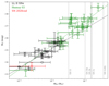 |
Fig. 13. Absolute V-band plateau magnitudes (computed at day 50) versus ejected nickel mass. Black circles represent the LL SN IIP sample (from Table 1), green squares are the SNe IIP from Hamuy (2003). SN 2020cxd is shown as a red data point. The grey dashed vertical lines represent the average nickel mass for different types of CC SNe from Anderson (2019). We perform linear fits on MV and log MNi for the Hamuy 2003 sample and for the LL SN IIP sample. The best fits are shown as the green and black dashed lines and give consistent relations. |
3.4. Host galaxy properties
The host galaxy of SN 2020cxd, NGC 6395, is classified as a Scd galaxy in NED and reported to have a stellar mass log M* = 9.29 ± 0.10 M⊙ by Leroy et al. (2019). This is close to the centre of the distribution of galaxy masses for SNe II hosts measured by Schulze et al. (2020) for the Palomar Transient Factory (PTF) sample (median log M* = 9.65 M⊙). Also, many of the other LL SNe have been discovered in large spirals (Spiro et al. 2014).
No metallicity measurement for NGC 6495 is reported in the literature. As described in Sect. 2.6, we therefore extracted the spectrum of a nearby H II region from the day 242 Keck spectrum in order to obtain a metallicity estimate. We measured the fluxes of a range of emission lines (Table 5) and used the flux ratios to calculate several common strong-line metallicity indicators using the pyMCZ code (Bianco et al. 2016). The Balmer decrement indicates a moderate extinction, E(B − V) = 0.36 ± 0.02 mag towards this H II region. We measured a slightly sub-solar metallicity in most indicators, for example we can adopt the N2 scale of the Pettini & Pagel (2004) calibration using the flux ratio between [N II] λ6583 and Hα. We found that 12 + log(O/H) = 8.50 ± 0.15. We also employed another metallicity diagnostic of Dopita et al. (2016) using [N II], Hα and [S II] lines, in which 12 + log(O/H) = 8.40 ± 0.10. Assuming a solar abundance of 8.69 (Asplund et al. 2009), the oxygen abundance of the host galaxy is  Z⊙. Compared to the stellar mass estimate of ∼109.29 M⊙ from Leroy et al. (2019), our metallicity is consistent with the galaxy mass-metallicity relation (e.g., Andrews & Martini 2013).
Measured relative galaxy emission line fluxes.
4. Summary and conclusions
In this work, we present SN 2020cxd, a LL SN IIP discovered by the ZTF that has one of the longest plateaus, the slowest ejecta, and the coolest photospheres among such known objects. The LC is well-sampled with a well determined explosion epoch and shows an initial sharp rise, and then a negative slope (s2) during the plateau phase, which peaks after about 100 days. The long-duration (118 days, OPTd) plateau ends with a very sharp drop to a low-luminosity radioactive tail, implying 0.003 M⊙ of 56Ni being ejected in the explosion. We find no evidence for a precursor at the site of the explosion, which is measured to have a slightly sub-solar metallicity.
We compare the nebular spectra to spectral synthesis models to constrain the progenitor mass through the [O I] λ6300, 6364 lines, and find relatively good agreements with progenitors of 12 and 15 M⊙, excluding more massive progenitor scenarios. This is an argument against a high mass (25 − 40 M⊙) RSG (as a Fe CC SN) with large amounts of material from the Ni-rich region falling back onto the newly formed degenerate core (Zampieri et al. 2003).
We constructed the bolometric LC of SN 2020cxd, and estimated a total radiated energy of Erad = 1.52 × 1048 erg over the first 200 days. The semi-analytic modelling suggests that SN 2020cxd originates from a progenitor which ejected about 9.5 M⊙ of ejecta. Although we cannot conclusively determine the explosion mechanism (electron capture or Fe CC) or the nature of the progenitor, all evidence are consistent with a Fe CC of a progenitor with a ZAMS mass on the order of 12 M⊙.
This presentation provides an observational account of SN 2020cxd, which warrants a detailed investigation given its unique position in the larger systematic BTS survey. We have argued that this SN is most likely the result of a CC in a low-ZAMS-mass star. This is in accordance with the notion that the low-luminosity tail of the SN luminosity function is underexplored and that improving the general understanding of the SN progenitor IMF requires further studies of large, well-controlled samples in tandem with detailed studies of individual examples to connect them to the stellar progenitors.
Following the methods of Bruch et al. (2021), we found there were not enough early phase data in either band to perform a power-law fit, and we thus set the explosion epoch as the mean of the first detection and the last non-detection.
SNOoPy is a package for SN photometry using PSF fitting and template subtraction developed by E. Cappellaro. A package description can be found at http://sngroup.oapd.inaf.it/snoopy.html.
Via scipy.find_peaks.
https://heasarc.gsfc.nasa.gov/docs/software/heasoft/ version 6.26.1.
With SN 2020cxd in the g band, whereas their sample was in V band.
As done by Anderson et al. (2014), we fit g-band data using a χ2 minimising procedure with a composed function of Gaussian, Fermi Dirac and straight line, following Olivares et al. (2010), from the estimated time of explosion.
As shown in Anderson et al. (2014, their Fig. 2), the mean of the s2 distribution is 1.27 mag per 100 days with a variance of 0.93 mag. The s2 slope of SN 2020cxd is 2.2σ off the distribution. However, there are a few SNe in their sample with similarly negative s2. We have been made aware, however, that such a negative plateau slope might be more common among the LL SNe II; see e.g., SN 1999br (Pastorello et al. 2004), SN 2009N (Takáts et al. 2014) and SNe 2013K and 2013am (Tomasella et al. 2018).
The Vega/AB magnitude conversion follows Blanton & Roweis (2007).
Could also be blended with He I λ5876, (see e.g., Pastorello et al. 2006, their Fig. 5).
IRAF is distributed by the National Optical Astronomy Observatories, which are operated by the Association of Universities for Research in Astronomy, Inc., under a cooperative agreement with the National Science Foundation.
For a specific line, we fit it with a Gaussian and integrated the flux using the trapezoidal rule over the Gaussian range above the continuum.
Note, however, that their original value for the explosion energy of SN 2018hwm is too low due to a numerical error (private communication, see also their errata from April 2021); their errata suggests 0.075 foe; our MCMC estimate is instead 0.23 foe for SN 2018hwn.
Acknowledgments
Based on observations obtained with the Samuel Oschin Telescope 48-inch and the 60-inch Telescope at the Palomar Observatory as part of the Zwicky Transient Facility project. ZTF is supported by the National Science Foundation under Grant No. AST-1440341 and a collaboration including Caltech, IPAC, the Weizmann Institute for Science, the Oskar Klein Center at Stockholm University, the University of Maryland, the University of Washington, Deutsches Elektronen–Synchrotron and Humboldt University, Los Alamos National Laboratories, the TANGO Consortium of Taiwan, the University of Wisconsin at Milwaukee, and Lawrence Berkeley National Laboratories. Operations are conducted by COO, IPAC, and UW. The SED Machine is based upon work supported by the National Science Foundation under Grant No. 1106171. This work was supported by the GROWTH (Kasliwal et al. 2019) project funded by the National Science Foundation under Grant No. 1545949. Partially based on observations made with the Nordic Optical Telescope, operated at the Observatorio del Roque de los Muchachos, La Palma, Spain, of the Instituto de Astrofisica de Canarias. Some of the data presented here were obtained with ALFOSC, which is provided by the Instituto de Astrofisica de Andalucia (IAA) under a joint agreement with the University of Copenhagen and NOTSA. This research has made use of the SIMBAD database, operated at CDS, Strasbourg, France, and of the NASA/IPAC Extragalactic Database (NED), which is operated by the Jet Propulsion Laboratory, California Institute of Technology, under contract with the National Aeronautics and Space Administration. MMK acknowledges generous support from the David and Lucille Packard Foundation. SY acknowledges support from the G.R.E.A.T research environment, funded by Vetenskapsrådet, the Swedish Research Council, project number 2016-06012. MR has received funding from the European Research Council (ERC) under the European Union’s Horizon 2020 research and innovation programme (grant agreement no. 759194 – USNAC). We thank Peter Nugent for comments on the manuscript. We thank the referee for a thorough read, and a reminder about the negative plateau slope seen in many LL SNe II.
References
- Ahn, C. P., Alexandroff, R., Allende Prieto, C., et al. 2014, ApJS, 211, 17 [NASA ADS] [CrossRef] [Google Scholar]
- Anderson, J. P. 2019, A&A, 628, A7 [NASA ADS] [CrossRef] [EDP Sciences] [Google Scholar]
- Anderson, J. P., González-Gaitán, S., Hamuy, M., et al. 2014, ApJ, 786, 67 [Google Scholar]
- Andrews, B. H., & Martini, P. 2013, ApJ, 765, 140 [NASA ADS] [CrossRef] [Google Scholar]
- Arnett, W. D., & Fu, A. 1989, ApJ, 340, 396 [NASA ADS] [CrossRef] [Google Scholar]
- Asplund, M., Grevesse, N., Sauval, A. J., & Scott, P. 2009, ARA&A, 47, 481 [NASA ADS] [CrossRef] [Google Scholar]
- Barker, B. L., Harris, C. E., Warren, M. L., O’Connor, E. P., & Couch, S. M. 2021, ApJ, submitted [arXiv:2102.01118] [Google Scholar]
- Bellm, E. C., Kulkarni, S. R., Graham, M. J., et al. 2019, PASP, 131, 018002 [Google Scholar]
- Benetti, S., Turatto, M., Balberg, S., et al. 2001, MNRAS, 322, 361 [NASA ADS] [CrossRef] [Google Scholar]
- Bianco, F. B., Modjaz, M., Oh, S. M., et al. 2016, Astron. Comput., 16, 54 [NASA ADS] [CrossRef] [Google Scholar]
- Blagorodnova, N., Neill, J. D., Walters, R., et al. 2018, PASP, 130, 5003 [Google Scholar]
- Blanton, M. R., & Roweis, S. 2007, AJ, 133, 734 [NASA ADS] [CrossRef] [Google Scholar]
- Blinnikov, S. I., & Popov, D. V. 1993, A&A, 274, 775 [NASA ADS] [Google Scholar]
- Breeveld, A. A., Landsman, W., & Holland, S. T. 2011, in American Institute of Physics Conference Series, eds. J. E. McEnery J. L. Racusin, & N. Gehrels, AIP Conf. Ser., 1358, 373 [NASA ADS] [Google Scholar]
- Bruch, R. J., Gal-Yam, A., Schulze, S., et al. 2021, ApJ, 912, 46 [NASA ADS] [CrossRef] [Google Scholar]
- Cardelli, J. A., Clayton, G. C., & Mathis, J. S. 1989, ApJ, 345, 245 [Google Scholar]
- Cenko, S. B., Fox, D. B., Moon, D.-S., et al. 2006, PASP, 118, 1396 [Google Scholar]
- De, K., Kasliwal, M. M., Tzanidakis, A., et al. 2020, ApJ, 905, 58 [NASA ADS] [CrossRef] [Google Scholar]
- Dekany, R., Smith, R. M., Riddle, R., et al. 2020, PASP, 132, 038001 [NASA ADS] [CrossRef] [Google Scholar]
- Dessart, L., & Hillier, D. J. 2005, A&A, 439, 671 [NASA ADS] [CrossRef] [EDP Sciences] [Google Scholar]
- Dessart, L., Hillier, D. J., Waldman, R., & Livne, E. 2013, MNRAS, 433, 1745 [NASA ADS] [CrossRef] [Google Scholar]
- Dopita, M. A., Kewley, L. J., Sutherland, R. S., & Nicholls, D. C. 2016, Ap&SS, 361, 61 [NASA ADS] [CrossRef] [Google Scholar]
- Eastman, R. G., Schmidt, B. P., & Kirshner, R. 1996, ApJ, 466, 911 [NASA ADS] [CrossRef] [Google Scholar]
- Fang, Q., & Maeda, K. 2018, ApJ, 864, 47 [NASA ADS] [CrossRef] [Google Scholar]
- Fraser, M., Ergon, M., Eldridge, J. J., et al. 2011, MNRAS, 417, 1417 [NASA ADS] [CrossRef] [Google Scholar]
- Fremling, C., Sollerman, J., Taddia, F., et al. 2016, A&A, 593, A68 [NASA ADS] [CrossRef] [EDP Sciences] [Google Scholar]
- Fremling, C., Miller, A. A., Sharma, Y., et al. 2020, ApJ, 895, 32 [NASA ADS] [CrossRef] [Google Scholar]
- Galbany, L., Hamuy, M., Phillips, M. M., et al. 2016, AJ, 151, 33 [NASA ADS] [CrossRef] [Google Scholar]
- Gal-Yam, A., Kasliwal, M. M., Arcavi, I., et al. 2011, ApJ, 736, 159 [NASA ADS] [CrossRef] [Google Scholar]
- Gehrels, N., Chincarini, G., Giommi, P., et al. 2004, ApJ, 611, 1005 [Google Scholar]
- Graham, M. J., Kulkarni, S. R., Bellm, E. C., et al. 2019, PASP, 131, 1001 [Google Scholar]
- Gutiérrez, C. P., Anderson, J. P., Hamuy, M., et al. 2017, ApJ, 850, 89 [CrossRef] [Google Scholar]
- Hamuy, M. 2003, ApJ, 582, 905 [NASA ADS] [CrossRef] [Google Scholar]
- Hamuy, M., Pinto, P. A., Maza, J., et al. 2001, ApJ, 558, 615 [NASA ADS] [CrossRef] [Google Scholar]
- Hiramatsu, D., Howell, D. A., & Van Dyk, S. D. 2021, Nat. Astron., 5, 903 [NASA ADS] [CrossRef] [Google Scholar]
- Horiuchi, S., Beacom, J. F., Kochanek, C. S., et al. 2011, ApJ, 738, 154 [NASA ADS] [CrossRef] [Google Scholar]
- Jäger, Z., Jr., Vinkó, J., & Bíró, B. I. 2020, MNRAS, 496, 3725 [CrossRef] [Google Scholar]
- Jerkstrand, A., Fransson, C., Maguire, K., et al. 2012, A&A, 546, A28 [NASA ADS] [CrossRef] [EDP Sciences] [Google Scholar]
- Jerkstrand, A., Smartt, S. J., Fraser, M., et al. 2014, MNRAS, 439, 3694 [Google Scholar]
- Jerkstrand, A., Ertl, T., Janka, H. T., et al. 2018, MNRAS, 475, 277 [Google Scholar]
- Kasen, D., & Woosley, S. E. 2009, ApJ, 703, 2205 [NASA ADS] [CrossRef] [Google Scholar]
- Kasliwal, M. M., Cannella, C., Bagdasaryan, A., et al. 2019, PASP, 131, 038003 [NASA ADS] [CrossRef] [Google Scholar]
- Leonard, D. C., Filippenko, A. V., Gates, E. L., et al. 2002, PASP, 114, 35 [Google Scholar]
- Leroy, A. K., Sandstrom, K. M., Lang, D., et al. 2019, ApJS, 244, 24 [Google Scholar]
- Lisakov, S. M., Dessart, L., Hillier, D. J., Waldman, R., & Livne, E. 2016, MNRAS, 466, 34 [Google Scholar]
- Lyman, J. D., Bersier, D., & James, P. A. 2013, MNRAS, 437, 3848 [Google Scholar]
- Maeda, K., Kawabata, K., Tanaka, M., et al. 2007, ApJ, 658, L5 [NASA ADS] [CrossRef] [Google Scholar]
- Martinez, L., Bersten, M. C., Anderson, J. P., et al. 2020, A&A, 642, A143 [NASA ADS] [CrossRef] [EDP Sciences] [Google Scholar]
- Masci, F. J., Laher, R. R., Rusholme, B., et al. 2019, PASP, 131, 018003 [Google Scholar]
- Mattila, S., Smartt, S. J., Eldridge, J. J., et al. 2008, ApJ, 688, L91 [NASA ADS] [CrossRef] [Google Scholar]
- Morozova, V., Piro, A. L., & Valenti, S. 2017, ApJ, 838, 28 [NASA ADS] [CrossRef] [Google Scholar]
- Müller-Bravo, T. E., Gutiérrez, C. P., Sullivan, M., et al. 2020, MNRAS, 497, 361 [Google Scholar]
- Nadyozhin, D. K. 2003, MNRAS, 346, 97 [NASA ADS] [CrossRef] [Google Scholar]
- Nagy, A. P., & Vinkó, J. 2016, A&A, 589, A53 [NASA ADS] [CrossRef] [EDP Sciences] [Google Scholar]
- Nagy, A. P., Ordasi, A., Vinkó, J., & Wheeler, J. C. 2014, A&A, 571, A77 [NASA ADS] [CrossRef] [EDP Sciences] [Google Scholar]
- Nakaoka, T., Kawabata, K. S., Maeda, K., et al. 2018, ApJ, 859, 78 [NASA ADS] [CrossRef] [Google Scholar]
- Nakar, E., Poznanski, D., & Katz, B. 2016, ApJ, 823, 127 [CrossRef] [Google Scholar]
- Nordin, J., Brinnel, V., Giomi, M., et al. 2020, Transient Name Server Discovery Report, 2020–555, 1 [Google Scholar]
- Olivares, E. F., Hamuy, M., & Giuliano, P. 2010, ApJ, 715, 833 [NASA ADS] [CrossRef] [Google Scholar]
- O’Neill, D., Kotak, R., Fraser, M., et al. 2021, A&A, 645, L7 [NASA ADS] [CrossRef] [EDP Sciences] [Google Scholar]
- Pastorello, A., Zampieri, L., Turatto, M., et al. 2004, MNRAS, 347, 74 [Google Scholar]
- Pastorello, A., Sauer, D., Taubenberger, S., et al. 2006, MNRAS, 370, 1752 [NASA ADS] [CrossRef] [Google Scholar]
- Pastorello, A., Valenti, S., Zampieri, L., et al. 2009, MNRAS, 394, 2266 [Google Scholar]
- Perley, D. 2020, Transient Name Server Classification Report, 2020–576, 1 [Google Scholar]
- Perley, D. A., Fremling, C., Sollerman, J., et al. 2020a, ApJ, 904, 35 [NASA ADS] [CrossRef] [Google Scholar]
- Perley, D. A., Taggart, K., Dahiwale, A., & Fremling, C. 2020b, Transient Name Server Classification Report, 2020–1503, 1 [Google Scholar]
- Pettini, M., & Pagel, B. E. J. 2004, MNRAS, 348, L59 [NASA ADS] [CrossRef] [Google Scholar]
- Popov, D. V. 1993, ApJ, 414, 712 [NASA ADS] [CrossRef] [Google Scholar]
- Pumo, M. L., Zampieri, L., Spiro, S., et al. 2016, MNRAS, 464, 3013 [Google Scholar]
- Reguitti, A., Pumo, M. L., Mazzali, P. A., et al. 2021, MNRAS, 501, 1059 [Google Scholar]
- Rigault, M., Neill, J. D., Blagorodnova, N., et al. 2019, A&A, 627, A115 [NASA ADS] [CrossRef] [EDP Sciences] [Google Scholar]
- Roming, P. W. A., Kennedy, T. E., Mason, K. O., et al. 2005, Space Sci. Rev., 120, 95 [Google Scholar]
- Roy, R., Kumar, B., Benetti, S., et al. 2011, ApJ, 736, 76 [NASA ADS] [CrossRef] [Google Scholar]
- Schlafly, E. F., & Finkbeiner, D. P. 2011, ApJ, 737, 103 [Google Scholar]
- Schulze, S., Yaron, O., Sollerman, J., et al. 2021, ApJS, 255, 29 [NASA ADS] [CrossRef] [Google Scholar]
- Smartt, S. J., Eldridge, J. J., Crockett, R. M., & Maund, J. R. 2009, MNRAS, 395, 1409 [CrossRef] [Google Scholar]
- Spiro, S., Pastorello, A., Pumo, M. L., et al. 2014, MNRAS, 439, 2873 [Google Scholar]
- Strotjohann, N. L., Ofek, E. O., Gal-Yam, A., et al. 2021, ApJ, 907, 99 [NASA ADS] [CrossRef] [Google Scholar]
- Sukhbold, T., Ertl, T., Woosley, S. E., Brown, J. M., & Janka, H. T. 2016, ApJ, 821, 38 [NASA ADS] [CrossRef] [Google Scholar]
- Takáts, K., Pumo, M. L., Elias-Rosa, N., et al. 2014, MNRAS, 438, 368 [CrossRef] [Google Scholar]
- Tomasella, L., Cappellaro, E., Pumo, M. L., et al. 2018, MNRAS, 475, 1937 [NASA ADS] [CrossRef] [Google Scholar]
- Turatto, M., Mazzali, P. A., Young, T. R., et al. 1998, ApJ, 498, L129 [NASA ADS] [CrossRef] [Google Scholar]
- Van Dyk, S. D., Davidge, T. J., Elias-Rosa, N., et al. 2012, AJ, 143, 19 [NASA ADS] [CrossRef] [Google Scholar]
- Yao, Y., Miller, A. A., Kulkarni, S. R., et al. 2019, ApJ, 886, 152 [NASA ADS] [CrossRef] [Google Scholar]
- Yaron, O., & Gal-Yam, A. 2012, PASP, 124, 668 [Google Scholar]
- Zampieri, L., Pastorello, A., Turatto, M., et al. 2003, MNRAS, 338, 711 [NASA ADS] [CrossRef] [Google Scholar]
- Zhang, J., Wang, X., Mazzali, P. A., et al. 2014, ApJ, 797, 5 [NASA ADS] [CrossRef] [Google Scholar]
Appendix A: Diluted blackbody fit
We fit a diluted blackbody (BB) function with multiple bands using the following formula:
 (A.1)
(A.1)
where Fλ is the flux at wavelength λ, B is the Planck function, Aλ is the extinction, T is the temperature, R is the radius, d is the distance, and ϵ is the dilution factor (Eastman et al. 1996; Hamuy et al. 2001; Dessart & Hillier 2005) that represents a general correction between the fitted BB distribution to the observed fluxes. We use the values from Dessart & Hillier (2005).
We also compare the absolute calibrated spectra of SN 2020cxd to the gri constructed BB functions. We integrated the de-reddened fluxes over the spectral bands using the trapezoidal rule, and calculated the ratio with the gri inferred fluxes. This method gives consistent results at early phases (ratio variance is small), but it does not work well in the nebular phase when the spectra become dominated by emission lines rather than the continuum.
Jäger et al. (2020) compared fluxes inferred from diluted BB functions (from VRI) to those directly integrated including infrared (IR) data (JHK) for a sample of LL SNe II. As shown in Jäger et al. (2020, their Fig. 4) BB fitting with optical bands agrees well with the results from direct integration of the full dataset. We also checked this with SN 2018hwm. As shown in Reguitti et al. (2021, their Fig. 2), SN 2018hwm was routinely followed by ZTF in g and r until ∼ 60 rest frame days, and was thereafter observed in multiple bands up to 200 days. We fit diluted BBs to the GP interpolated optical and IR photometry of SN 2018hwm every 2 days during this period. For each epoch, we calculated the ratio between the gri inferred BB fluxes to those obtained by directly integrating the optical and JHK spectral energy distributions (SED), and found the differences are always less than 10%, which supports the validity of the Jäger et al. (2020) approach.
In the UV region, Jäger et al. (2020) extrapolate to 2000 Å from the B and V bands, assuming zero flux for even shorter wavelengths (Lyman et al. 2013). For SN 2020cxd, we have six epochs of Swift UVOT data, and can thus integrate the luminosity directly with the UV bands. As shown in the six subplots of Fig. B.1, we compare the gri constructed BB to those inferred from using the full dataset including the Swift UV data. The gri inferred BB luminosities are similar to those obtained from the full dataset as well.
We adopt the BB fitting method to estimate the bolometric LC of SN 2020cxd during its photospheric phase, and this is shown as a black dashed line in Fig. C.1. The dark orange shaded region in that figure represents the errors from the distance uncertainty, while the light orange area stands for the errors from the uncertainty of temperature of the fitted BB. For comparison, we also show the spectra integrated luminosity (green crosses) and gri+UV inferred luminosity (red crosses) in Fig. C.1.
Appendix B: Bolometric correction method
The BC is defined as:
 (B.1)
(B.1)
where Mbol is the bolometric magnitudes, and Mx is the absolute magnitude of SN 2020cxd in filter x. Jäger et al. (2020, their Fig. 5) compare the BCB of the LL SN sample to show their similarity, which supports the validity of the empirical correlation found by Lyman et al. (2013). We show the BCg evolution of SN 2020cxd (as derived from our BB fits for the first 140 days) and of SN 2018hwm in Fig. B.2. Lyman et al. (2013) fitted BCg as a function of (g − r)/(g − i) colors for a sample of Type II SNe, which is also shown as the red (for early phase) and green (for the nebular phase) dashed lines for comparison. The BCg evolution of SN 2020cxd is similar to that of SN 2018hwm, and also to that from the Lyman model during the optically thick phase. Since the color of LL Type IIP SNe in the nebular phase is outside the fitting range of the Lyman model (the green dashed line), we use the BCg of SN 2018hwm to estimate the bolometric LC of SN 2020cxd in the nebular phase, shown as the blue dashed line in Fig. C.1. In fact, it is the BCr for SN 2018hwm that we use for SN 2020cxd, since we do not have g-band data on the tail. The dark blue shaded region corresponds to the errors from the distance uncertainty of SN 2020cxd, while the light blue shaded area marks the errors from the BB fitting and validity.
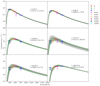 |
Fig. B.1. Blackbody fitting comparisons for SN 2020cxd. The six subplots compare the gri+UV constructed BB at the six epochs when Swift UVOT data are available to the gri inferred ones. Best fits of the full dataset are shown as the black dashed lines and the 3σ uncertainties are overplotted as the grey shaded regions. Best fits and errors of the gri dataset are instead shown as green dashed lines and shaded areas. The rest frame phase, as well as the ratio between the integrated luminosities of the full and gri datasets, are provided to the right in each subplot. |
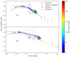 |
Fig. B.2. Bolometric correction of SN 2020cxd in the g band versus g − r (upper panel) and g − i (lower panel) colors. We have also included the corrections for SN 2018hvm as well as the comparison to the BC from Lyman et al. (2013). Overall, these are all similar which makes us confident in the applied corrections for SN 2020cxd. |
Appendix C: Monto carlo fitting code with semi-analytic models
This code was first developed by Nagy & Vinkó (2016), which generate modelled LCs of CC SNe for a variety of parameters e.g. the ejected mass, the initial progenitor radius, the total explosion energy, and the synthesized nickel mass (following early work of Arnett & Fu 1989; Popov 1993; Blinnikov & Popov 1993; Nagy et al. 2014), and was further developed by Jäger et al. (2020) who added a markov chain monte carlo (MCMC) method. The model is based on a two-component configuration consisting of a uniform dense stellar core and an extended low-mass envelope where the density decreases as an exponential function. After comparison, Nagy & Vinkó (2016) conclude that the results from the two-component semi-analytic LC model are consistent with current state-of-the-art calculations for Type II SNe, so the estimated fitting parameters can be used for preliminary studies awaiting more sophisticated hydrodynamic modelling.
We also compared the semi-analytic fitting results from Jäger et al. (2020) to hydrodynamical modelling results from Martinez et al. (2020), and found that the estimated ejecta masses are similar. For SN 2005cs, the best-fit ejecta mass with the analytic model is 8.84 M⊙, which is similar to the hydrodynamical result of 8 M⊙. For SN 2004et, the estimated ejecta masses of the semi-analytic and hydrodynamical models are both 13 M⊙. As an additional test, we fit SN 2018hwm with the semi-analytic LC fitting code, and obtain 7.6 ± 1.3 M⊙ for the ejecta mass, which is consistent with the hydrodynamic modelling result of Reguitti et al. (2021) of 8 M⊙. These comparisons provide some confidence in the derived ejecta masses from the simple analytical fits provided here. The fits to the LC of SN 2020cxd are shown in Fig. C.1.
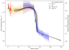 |
Fig. C.1. SN 2020cxd LC comparison between observations and sampled MCMC fits (solid black lines). The black dashed line represents the observed LC of SN 2020cxd at early phases from BB fitting, with the orange shaded region as errors from the distance uncertainty (dark) and from the fitted BB (light). The blue dashed line is the observed LC of SN 2020cxd at later epochs from the BC approach, with the blue shaded region as errors from the distance uncertainty (dark) and the fitted BB (light). The green crosses stands for the epochs with fluxes from direct spectral integration, while the red crosses is from BB fits with gri+UV photometry. |
All Tables
All Figures
|
Fig. 1. SN 2020cxd in the nearby galaxy NGC 6395. The g-band image subtraction is shown in the top panels (subtraction to the right), with the SN image observed on 24 April 2020 – 64.9 days after the first ZTF detection (to the left). Bottom panel: a gri-colour composite image of the host galaxy and its environment. It was composed of ZTF g-, r- and i-band pre-explosion images of the field. |
| In the text | |
|
Fig. 2. Light curves of SN 2020cxd in the g (green symbols), r (red), and i (black) bands. These are host-subtracted magnitudes from the P48, P60, and LT, as well as two epochs from the NOT on the late tail. Forced photometry obtained using SNOoPY is plotted as open circles. All are observed (AB) magnitudes in the observer frame in days since the explosion. Relevant upper limits are displayed as inverted triangles, and constrain the explosion epoch of the SN (the purple vertical dashed line), as well as the g-band tail. The dashed lines with error regions are Gaussian process estimates of the interpolated and extrapolated LC. After 150 days, we show the linear fits instead. The yellow downward pointing arrows on top indicate the epochs of spectroscopy, the blue vertical bars display the epochs with Swift observations. |
| In the text | |
|
Fig. 3. ZTF P48 pre-explosion images for SN 2020cxd reveal no precursors in g (green symbols), r (red), or i (black) bands. Filled data points are ≳ 5σ detections, whereas arrows show 5σ upper limits. The data are binned in seven-day bins. |
| In the text | |
|
Fig. 4. Sequence of optical spectra for SN 2020cxd, corrected for redshift and reddening. The complete log of spectra is provided in Table 4. The epoch (rest frame days since explosion) of the spectra is provided to the right. The spectra are shifted in flux by a constant for clarity. Late time spectra are scaled for comparison. The scaling factors are also listed to the right. Some spectra are also binned (shown as black lines), with a window size of 5 Å for LT, and 10 Å for NOT/Gemini/Keck, and their original spectra are shown in shaded grey. |
| In the text | |
|
Fig. 5. Absolute magnitudes of SN 2020cxd (black stars) together with the LCs of other LL SNe IIP, as well as for the normal Type II SN 1999em (green circles). We highlight SN 2013am (orange circles) which is the brightest within the LL SN II sample, and SNe 1999eu (purple circles) and 1999br (blue circles) which are the faintest. We also use a larger marker for SN 2018hwm (red hexagons), which was also monitored by ZTF in gri photometry. The other SNe are displayed with smaller and fainter markers. The LCs are plotted versus rest frame days past explosion. The radioactive cobalt decay rate is shown as a black line in the r- and i-band panels for comparison. The photometric data were obtained via the Open Supernova Catalog. Data reference for SN 1999em is Leonard et al. (2002), and for the LL SNe II these are listed in Table 1. |
| In the text | |
|
Fig. 6. Colour evolution of SN 2020cxd (black stars) shown in g − r (upper panel) and r − i (lower panel). The colours have been corrected for MW extinction. For comparison, we have also plotted colours for several other LL SNe II. Most of these are V − R and R − I. For references see Table 1. |
| In the text | |
|
Fig. 7. Sequence of early photospheric spectra for SN 2020cxd, compared with spectra of other LL Type IIP SNe in grey. The epoch of the spectrum is provided to the right. Some identified lines (H, Na I D and Ca NIR triplet) are marked as vertical dashed lines. We also mark several metal lines as short vertical lines, which might be present in the last P60 spectrum. |
| In the text | |
|
Fig. 8. Sequence of nebular spectra for SN 2020cxd, compared with spectra of other LL Type IIP SNe in grey. The epoch of the spectrum is provided to the right. Some identified lines, e.g., Hα, [Ca II] λλ7291, 7323, Ca II NIR triplet, [O I] λλ6300, 6364, and λ8446, are marked as vertical dashed lines. |
| In the text | |
|
Fig. 9. Velocity evolution of SN 2020cxd. Upper panel shows the expansion velocities estimated from Hα P-Cygni minima (black stars) and FWHM (red stars), Hβ P-Cygni minima (yellow squares), [Ca II] λ7291 line FWHM (blue cross), FWHM of Ca II NIR triplet middle line (green diamonds), and [O I] λ6300 line FWHM (orange pentagons). Hα velocities for SN 2020cxd compared to other LL SNe discussed throughout the paper. A comparison with the normal Type II SN 1999em is shown in the lower panel. The x-axis shows the phase with respect to explosion. Line velocities of the other LL SNe II are taken from Pastorello et al. (2004) to Spiro et al. (2014). |
| In the text | |
|
Fig. 10. Comparison between the last Keck spectrum of SN 2020cxd at nebular phases and scaled synthetic spectra. The black curves are the observed spectra, binned with a window size of 10 Å, and corrected for redshift and extinction. The models are displayed with coloured lines, and originate from Jerkstrand et al. (2012, 2014), Dessart et al. (2013), Lisakov et al. (2016). These were obtained via WISeREP. The models are scaled by nickel mass ratio. All model spectra are shifted to the SN distance by the inverse square of the distance. Their rest frame phases and scaling factors are shown in the legend. |
| In the text | |
|
Fig. 11. Bolometric luminosities of several LL SNe IIP and the famous SN 1987A. The luminosity of SN 2020cxd (shown as the red stars) was calculated after accounting for MW extinction and distance. The slope of the luminosity tail matches well with the radioactive decay of 56Co. |
| In the text | |
|
Fig. 12. Temperature and radius of several LL SNe IIP, including SN 2020cxd (shown as black stars). Upper panel: evolution of their photospheric temperature estimated by fitting a blackbody to the SED in the optically thick phase. Bottom panel: evolution of their photospheric radius based on the same fits. We followed Jäger et al. (2020) in the methodology and the included SNe are also from that paper. |
| In the text | |
|
Fig. 13. Absolute V-band plateau magnitudes (computed at day 50) versus ejected nickel mass. Black circles represent the LL SN IIP sample (from Table 1), green squares are the SNe IIP from Hamuy (2003). SN 2020cxd is shown as a red data point. The grey dashed vertical lines represent the average nickel mass for different types of CC SNe from Anderson (2019). We perform linear fits on MV and log MNi for the Hamuy 2003 sample and for the LL SN IIP sample. The best fits are shown as the green and black dashed lines and give consistent relations. |
| In the text | |
|
Fig. B.1. Blackbody fitting comparisons for SN 2020cxd. The six subplots compare the gri+UV constructed BB at the six epochs when Swift UVOT data are available to the gri inferred ones. Best fits of the full dataset are shown as the black dashed lines and the 3σ uncertainties are overplotted as the grey shaded regions. Best fits and errors of the gri dataset are instead shown as green dashed lines and shaded areas. The rest frame phase, as well as the ratio between the integrated luminosities of the full and gri datasets, are provided to the right in each subplot. |
| In the text | |
|
Fig. B.2. Bolometric correction of SN 2020cxd in the g band versus g − r (upper panel) and g − i (lower panel) colors. We have also included the corrections for SN 2018hvm as well as the comparison to the BC from Lyman et al. (2013). Overall, these are all similar which makes us confident in the applied corrections for SN 2020cxd. |
| In the text | |
|
Fig. C.1. SN 2020cxd LC comparison between observations and sampled MCMC fits (solid black lines). The black dashed line represents the observed LC of SN 2020cxd at early phases from BB fitting, with the orange shaded region as errors from the distance uncertainty (dark) and from the fitted BB (light). The blue dashed line is the observed LC of SN 2020cxd at later epochs from the BC approach, with the blue shaded region as errors from the distance uncertainty (dark) and the fitted BB (light). The green crosses stands for the epochs with fluxes from direct spectral integration, while the red crosses is from BB fits with gri+UV photometry. |
| In the text | |
Current usage metrics show cumulative count of Article Views (full-text article views including HTML views, PDF and ePub downloads, according to the available data) and Abstracts Views on Vision4Press platform.
Data correspond to usage on the plateform after 2015. The current usage metrics is available 48-96 hours after online publication and is updated daily on week days.
Initial download of the metrics may take a while.