The GUAPOS project

L. Colzi; V. M. Rivilla; M. T. Beltrán; I. Jiménez-Serra; C. Mininni; M. Melosso; R. Cesaroni; F. Fontani; A. Lorenzani; A. Sánchez-Monge; S. Viti; P. Schilke; L. Testi; E. R. Alonso; L. Kolesniková

doi:10.1051/0004-6361/202141573

Home

All issues

Volume 653 (September 2021)

A&A, 653 (2021) A129

Full HTML

Free Access

Issue		A&A Volume 653, September 2021


Article Number		A129
Number of page(s)		45
Section		Interstellar and circumstellar matter
DOI		https://doi.org/10.1051/0004-6361/202141573
Published online		22 September 2021

A&A 653, A129 (2021)

II. A comprehensive study of peptide-like bond molecules^★

L. Colzi¹^,2, V. M. Rivilla¹^,2, M. T. Beltrán², I. Jiménez-Serra¹, C. Mininni²^,3^,4, M. Melosso⁵, R. Cesaroni², F. Fontani², A. Lorenzani², A. Sánchez-Monge⁶, S. Viti⁷, P. Schilke⁶, L. Testi²^,8, E. R. Alonso⁹ and L. Kolesniková⁹^,10

¹ Centro de Astrobiología (CSIC-INTA), Ctra. de Ajalvir Km. 4, 28850, Torrejón de Ardoz, Madrid, Spain
e-mail: lcolzi@cab.inta-csic.es
² INAF-Osservatorio Astrofisico di Arcetri, Largo E. Fermi 5, 50125, Florence, Italy
³ Università degli studi di Firenze, Dipartimento di fisica e Astronomia, Via Sansone 1, 50019 Sesto Fiorentino, Italy
⁴ INAF-IAPS, via del Fosso del Cavaliere 100, 00133 Roma, Italy
⁵ Dipartimento di Chimica “Giacomo Ciamician”, Università di Bologna, Via F. Selmi 2, 40126 Bologna, Italy
⁶ I. Physikalisches Institut, Universität zu Köln, Zülpicher Str. 77, 50937 Köln, Germany
⁷ University of Leiden, Niels Bohrweg 2, 2333 CA Leiden, The Netherlands
⁸ European Southern Observatory, Karl-Schwarzschild-Strasse 2, 85748 Garching bei München, Germany
⁹ Grupo de Espectroscopia Molecular (GEM), Edificio Quifima, Área de Química-Física, Laboratorios de Espectroscopia y Bioespectroscopia, Parque Científico UVa, Unidad Asociada CSIC, Universidad de Valladolid, 47011 Valladolid, Spain
¹⁰ Department of Analytical Chemistry, University of Chemistry and Technology, Technická 5, 166 28 Prague 6, Czech Republic

Received: 16 June 2021
Accepted: 23 July 2021

Abstract

Context. Peptide-like bond molecules, which can take part in the formation of proteins in a primitive Earth environment, have been detected only towards a few hot cores and hot corinos up to now.

Aims. We present a study of HNCO, HC(O)NH₂, CH₃NCO, CH₃C(O)NH₂, CH₃NHCHO, CH₃CH₂NCO, NH₂C(O)NH₂, NH₂C(O)CN, and HOCH₂C(O)NH₂ towards the hot core G31.41+0.31. The aim of this work is to study these species together to allow a consistent study among them.

Methods. We have used the spectrum obtained from the ALMA 3 mm spectral survey GUAPOS, with a spectral resolution of ~0.488 MHz (~1.3–1.7 km s⁻¹) and an angular resolution of 1.′′2 × 1.′′2 (~4500 au), to derive column densities of all the molecular species presented in this work, together with 0.′′2 × 0.′′2 (~750 au) ALMA observations from another project to study the morphology of HNCO, HC(O)NH₂, and CH₃C(O)NH₂.

Results. We have detected HNCO, HC(O)NH₂, CH₃NCO, CH₃C(O)NH₂, and CH₃NHCHO, but no CH₃CH₂NCO, NH₂C(O)NH₂, NH₂C(O)CN, or HOCH₂C(O)NH₂. This is the first time that these molecules have been detected all together outside the Galactic centre. We have obtained molecular fractional abundances with respect to H₂ from 10⁻⁷ down to a few 10⁻⁹ and abundances with respect to CH₃OH from 10⁻³ to ~4 × 10⁻², and their emission is found to be compact (~2′′, i.e. ~7500 au). From the comparison with other sources, we find that regions in an earlier stage of evolution, such as pre-stellar cores, show abundances at least two orders of magnitude lower than those in hot cores, hot corinos, or shocked regions. Moreover, molecular abundance ratios towards different sources are found to be consistent between them within ~1 order of magnitude, regardless of the physical properties (e.g. different masses and luminosities), or the source position throughout the Galaxy. Correlations have also been found between HNCO and HC(O)NH₂ as well as CH₃NCO and HNCO abundances, and for the first time between CH₃NCO and HC(O)NH₂, CH₃C(O)NH₂ and HNCO, and CH₃C(O)NH₂ and HC(O)NH₂ abundances. These results suggest that all these species are formed on grain surfaces in early evolutionary stages of molecular clouds, and that they are subsequently released back to the gas phase through thermal desorption or shock-triggered desorption.

Key words: astrochemistry / line: identification / ISM: molecules / ISM: individual objects: G31.41+0.31 / stars: formation

^★

Table C.1 is only available at the CDS via anonymous ftp to cdsarc.u-strasbg.fr (130.79.128.5) or via http://cdsarc.u-strasbg.fr/viz-bin/cat/J/A+A/653/A129

© ESO 2021

1 Introduction

The study of the origin of life on Earth is one of the main challenges among biologists, chemists, geologists, and, in recent years, also astrophysicists. In fact, the advent of more sensitive and higher spatial and spectral resolution astronomical instruments, such as the Atacama Large Millimeter Array (ALMA), allowed the detection of ~240 molecular species in the interstellar medium (ISM), about 100 of which are complex organic molecules (COMs), that is molecules containing carbon with six or more atoms (McGuire 2018). In particular, COMs have been detected ubiquitously in the ISM towards high-mass and low-mass star-forming regions (e.g. Hollis et al. 2004; Beltrán et al. 2009; Belloche et al. 2013; Jørgensen et al. 2012), protostellar molecular outflows (e.g. Arce et al. 2008; Codella et al. 2020), photon-dominated regions (e.g. Guzmán et al. 2013; Cuadrado et al. 2017), dark clouds cores and pre-stellar cores (e.g. Marcelino et al. 2007; Bacmann et al. 2012; Jiménez-Serra et al. 2016), and Galactic Centre (GC) molecular clouds (e.g. Requena-Torres et al. 2006; Zeng et al. 2018; Rivilla et al. 2019, 2021; Jiménez-Serra et al. 2020).

Among prebiotic COMs, those containing peptide-like bonds (NCO backbone) are of great interest because they can participate in the link of amino acids forming proteins (e.g. Pascal et al. 2005). Peptide-like bond molecules detected to date in the ISM are isocyanic acid (HNCO), formamide (HC(O)NH₂), methyl isocyanate (CH₃NCO), acetamide (CH₃C(O)NH₂) and its isomer N-methylformamide (CH₃NHCHO), and urea (NH₂C(O)NH₂). Unlike these species, ethyl isocyanate (CH₃CH₂NCO), cyanoformamide (NH₂C(O)CN), and glycolamide (HOCH₂C(O)NH₂), which also contain the peptide-like bond, have never been detected in the ISM. Kolesniková et al. (2018) report the rotational spectrum of CH₃CH₂NCO from 80 to 340 GHz, and they searched for it towards the Orion KL and Sgr B2 hot molecular cores (HMCs) without success. Sanz-Novo et al. (2020) provided experimental frequencies of the rotational lines in the ground vibrational state of HOCH₂C(O)NH₂ and searched for it towards SgrB2(N) also without success. Finally, NH₂C(O)CN searches in the ISM have never been reported. Isocyanic acid, HNCO, was detected towards HMCs, low-mass protostars, translucent molecular clouds, molecular outflows, and extragalactic regions (e.g. Snyder & Buhl 1972; Turner et al. 1999; Helmich & van Dishoeck 1997; Bisschop et al. 2007; Zeng et al. 2018; Rodríguez-Fernández et al. 2010; Nguyen-Q-Rieu et al. 1991; Nazari et al. 2021; Canelo et al. 2021). Formamide, HC(O)NH₂, has been also detected towards many different high- and low-mass star-forming regions (e.g. López-Sepulcre et al. 2019). Methyl isocyanate, CH₃NCO was detected towards Sgr B2(N), Orion KL, the low-mass protostars IRAS 16293-2422 A and B, the high-mass protostellar object G328.2551-0.5321, the G10.47+0.03 and G31.41+0.31 HMCs, and the Serpens SMM1 hot corino (Halfen et al. 2015; Cernicharo et al. 2016; Martín-Doménech et al. 2017; Ligterink et al. 2017, 2018, 2021; Manigand et al. 2020; Csengeri et al. 2019; Gorai et al. 2020, 2021). Acetamide, CH₃C(O)NH₂, was detected towards different high-mass star-forming regions (Hollis et al. 2006; Halfen et al. 2011; Cernicharo et al. 2016; Belloche et al. 2017; Ligterink et al. 2020) and tentatively detected towards IRAS 16293-2422 B (Ligterink et al. 2018). Moreover, the second most stable C₂H₅NO isomer after CH₃C(O)NH₂, N-methylformamide, CH₃NHCHO (Lattelais et al. 2010), was detected towards Sgr B2(N1S) and NGC 6334I and tentatively detected towards SgrB2(N2) (Belloche et al. 2017, 2019; Ligterink et al. 2020). Recently, urea, NH₂C(O)NH₂, has been detected towards Sgr B2(N1) and the GC molecular cloud G+0.693-0.027 (Belloche et al. 2019; Jiménez-Serra et al. 2020), and tentatively detected towards NGC 7538 IRS9, Sgr B2(N-LMH), and NGC 6334I (Raunier et al. 2004; Remijan et al. 2014; Ligterink et al. 2020).

These peptide-like bond species have preferentially been detected so far in massive and clustered star-forming regions. In this sense, it is worth noting that our Sun is thought to have been formed in a clustered environment in the presence of massive stars (e.g Adams 2010; Lichtenberg et al. 2019; Wallner et al. 2020; Korschinek et al. 2020). Therefore, the study of the chemical reservoir of the birth environment of massive stars, known as HMCs, can give us important hints about the chemical heritage that our own Solar System received from its natal environment.

For all of these species, different chemical formation and destruction pathways, both on grain surfaces and in gas phase, have been proposed (e.g. Agarwal et al. 1985; Grim et al. 1989; Garrod et al. 2008; Jones et al. 2011; Noble et al. 2015; Fedoseev et al. 2016; Belloche et al. 2017; Quénard et al. 2018). However, chemical networks still need important new inputs from observationsin different astronomical environments to be properly constrained.

In this paper, we study molecules with one or more peptide-like bonds (see Fig. 1) towards the HMC G31.41+0.31 (hereafter G31) in the context of the G31 Unbiased ALMA sPectral Observational Survey (GUAPOS, Mininni et al. 2020). All these molecules are reported for the first time in this paper towards G31, with the exceptions of HC(O)NH₂, recently detected by Coletta et al. (2020) using single-dish data, and CH₃NCO, recently reported by Gorai et al. (2021). G31 is a HMC located at a distance of 3.75 kpc (Immer et al. 2019), with a luminosity of ~4.5 × 10⁴ L_⊙ (from Osorio et al. 2009) and a mass of ~70 M_⊙ (Cesaroni 2019). The core harbours two free-free continuum sources separated by ~0.′′2 (Cesaroni et al. 2010), and new VLA and ALMA observations show that there are at least four massive star-forming regions in the core (Beltrán et al. 2021). Moreover, few molecular lines present an inverse P-Cygni profile, indicating that the core is collapsing and rotating with respect to the direction of a magnetic field, revealed by polarisation measurements (Girart et al. 2009; Beltrán et al. 2019). G31 is an excellent source to search for complex molecules since it presents a very rich chemistry, as already shown by previous works (e.g. Beltrán et al. 2005, 2009, 2018; Rivilla et al. 2017; Mininni et al. 2020; Gorai et al. 2021). This is the second paper from this survey, after the first one which presented the GUAPOS project and the analysis of the three energetically most stable C₂H₄O₂ isomers (Mininni et al. 2020).

In Sects. 2 and 3, we present the observations and the results, respectively. In Sect. 4, we provide a detailed comparison with previous observations towards other sources and a discussion of the main formation and destruction reactions proposed for these species, giving new inputs for future chemical models. Finally, the conclusions are summarised in Sect. 5.

2 Observations and data analysis

2.1 ALMA data

Observations towards the HMC G31 were taken with ALMA during Cycle 5 (project 2017.1.00501.S, P.I.: M. T. Beltrán) obtaining an unbiased spectral survey in Band 3, from 84.05 GHz up to 115.91 GHz. The frequency resolution is 0.49 MHz, corresponding to a velocity resolution of ~1.6 km s⁻¹ at 90 GHz. The final angular resolution is ~1.′′2 (~4500 au). The root mean square (rms) noise of the maps varies between 0.5 mJy beam⁻¹ and 1.9 mJy beam⁻¹. The pointing centre of the observations is α_J2000 = 18^h47^m34^s and δ_J2000 = −0.1°12′45′′. The uncertainty on the flux calibration is of ~5%. For more details see Mininni et al. (2020).

In this work, as in Mininni et al. (2020), we have analysed a spectrum extracted inside an area equal to the beam size towards the continuum peak position (α_J2000 = 18^h 47^m34^s.321 and δ_J2000 = −0.1°12′45.′′977). The rms noise of the spectrum varies from 7 mK to 27 mK. The spectrum of G31 is very line rich, which prevents to subtract the continuum by simply using line-free channels. Thus, we have applied the corrected sigma clipping method (c-SMC) approach of the Python-based tool STATCONT¹ (Sánchez-Monge et al. 2018) to subtract the continuum. A detailed discussion of the results of this method is presented in Appendix A. The error associated with the final Band 3 spectrum is of ±1.2 K, which corresponds to the 11% of the continuum level at a reference frequency of 84.579 GHz. This error is included as an additional error on the parameters derived from the fit to the spectrum.

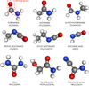Fig. 1

Chemical structure of the peptide-like bond molecules studied in this paper. White, grey, red, and blue spheres correspond to H, C, O, and N atoms, respectively.

2.2 Additional high-angular resolution data

Interferometric observations of G31 at higher angular resolution were carried out with ALMA in Cycle 2 in July and September 2015 as part of project 2013.1.00489.S. (P.I.: R. Cesaroni). The observations were carried out in Band 6 with the array in an extended configuration. The digital correlator was configured in thirteen spectral windows (SPW), one broad window for the continuum and twelve narrow ones for the lines, covering different bandwidths from ~217 GHz to ~236.5 GHz. The phase reference centre of the observations is α_J2000 = 18^h 47^m34^s.315, δ_J2000 = −01° 12′ 45.′′90. The resulting synthesised cleaned beam of the maps is 0.′′ 2 × 0.′′2 (~750 au) for the lines analysed in this work. The rms noise of the maps is ~1.3 mJy beam⁻¹ at ~217 GHz and 218 GHz, ~1.5 mJy beam⁻¹ at ~219 GHz, and ~2 mJy beam⁻¹ at ~220 GHz. We refer to Cesaroni et al. (2017) and Beltrán et al. (2018) for detailed information on the observations.

2.3 Spectral analysis

The line identification of the molecular species present in the GUAPOS spectrum has been done using the version 01/12/2020 of the SLIM (Spectral Line Identification and Modelling) tool within the MADCUBA package² (Martín et al. 2019). SLIM uses the spectroscopic entries from the Cologne Database for Molecular Spectroscopy³ (CDMS, Müller et al. 2001, 2005; Endres et al. 2016), the Jet Propulsion Laboratory⁴ (JPL, Pickett et al. 1998), and for species whose spectroscopy was not present in the catalogues we have added entries using available spectroscopic works. Then, SLIM generates a synthetic spectrum, assuming local thermodynamic equilibrium (LTE) conditions and taking into account the line opacity. In this study, we focused the analysis on the molecules containing one or more peptide-like bonds (NCO backbone) HNCO, HC(O)NH₂, CH₃NCO, CH₃C(O)NH₂, CH₃NHCHO, CH₃CH₂NCO, NH₂C(O)NH₂, NH₂C(O)CN, and HOCH₂C(O)NH₂ (Fig. 1). Details on the spectroscopic entries used for these species can be found in Appendix B. Beside the analysis of the peptide-like bond molecules, a preliminary identification of other molecular species has been done to evaluate theeffect of possible line contaminations (e.g. thin red line of Fig. 2). For each molecular species we used the MADCUBA-AUTOFIT tool to compare the observed spectrum with the LTE synthetic one. This fitting tool provides the best non-linear least-squared fit to all the transitions taken into account by using the Levenberg-Marquardt algorithm. The free parameters of the fitting are the column density of the molecule, N, the excitation temperature, T_ex, the peak velocity, v_LSR, and the full-width-half-maximum (FWHM), Δv. As described by Mininni et al. (2020), the LTE assumption is well justified because of the high volume density n(H₂) ~ 10⁸ cm⁻³. Since the emission of the HMC fills the beam (i.e. the region from which we have extracted the spectrum, see Sect. 3.2 and Mininni et al. 2020), we did not consider beam-dilution in the fitting procedure. Moreover, since we have also considered the possible contamination from other molecular species, we have limited the fit to non-contaminated or slightly contaminated transitions. In particular, we have considered (i) non-contamination from a line of another species if its peak is at a distance larger than FWHM from the peak of the considered line, and ii) in case of blending with peak separation <FWHM, the contamination of the line of the other species should be <15%. Thus, the parameters above are left free to obtain the best-LTE fit whenever the algorithm reaches the convergence. If convergence cannot be reached, FWHM, v_LSR, and/or T_ex have been fixed as explained in Sect. 3.1. When the algorithm converges, it also provides the errors on the parameters. The transitions used for the fit of each molecule are listed in Table C.1. When the spectroscopic information of vibrationally excited states is present, the total partition function used for the fit (Q_vibrot) has been derived taking into account the contribution of both the rotational partition function, Q_rot, and the vibrational one, Q_vib, Q_vibrot = Q_rot × Q_vib (see Appendix B). The final relative error on the total column densities has been derived as the square root of the quadratic sum of the relative error given by the fit algorithm and the error on the continuum level (11%, see Sect. 2.1). Finally, the molecular abundances (X) were derived using the column density of H₂, obtained from the continuum emission inside the area from which we extracted the spectrum, $N_{H_{2}}$ $N_{\textrm{H}_{2}}$ = (1.0 ± 0.2) × 10²⁵ cm⁻² (see Mininni et al. 2020).

The analysis of the different vibrational states has been done separately for HNCO, HC(O)NH₂, and CH₃NCO, because of the difficulty to fit all of the transitions of a molecule with a single T_ex. In fact, it is well know that the HMC G31 has a temperature gradient, with temperatures of ~100 K towards the outer part (at ~0.03 pc from the centre), and of ~450 K towards its centre (Beltrán et al. 2018). Moreover, as we discuss in Sects. 3.1.1, 3.1.2, and 3.1.3, the ground vibrational states of these molecules are optically thicker than the vibrationally excited ones. Thus, we only discuss the results obtained from the ¹³C-isotopologues, or from the vibrationally excited states if the ¹³C-isotopologues have not been detected. Conversely, the resulting fit for CH₃C(O)NH₂ was obtained taking into account the v = 0, and v_t = 1, 2 transitions all together, because we find that they all are optically thin. For CH₃NHCHO, only the ground vibrational state transitions have been detected and analysed, and upper limits will be provided for its excited states transitions. Finally, CH₃CH₂NCO, NH₂C(O)NH₂, NH₂C(O)CN, and HOCH₂C(O)NH₂ have not been detected, and only upper limits of the ground vibrational state will be provided.

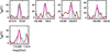Fig. 2

Transitions listed in Table C.1 and used to fit the v = 0 state of isocyanic acid (HNCO) and its ¹³C-isotopologue (HN¹³ CO). The magenta and green curves represent the best LTE fits obtained with MADCUBA for HNCO and HN¹³ CO, respectively (Table 1). The red curve shows the simulated spectrum taking into account all the species identified so far in the region.

3 Results

In this section, we show the results obtained from the line fitting procedure performed with MADCUBA-SLIM for the nine species (Sects. 3.1.1–3.1.6 and Appendix D). The non-contaminated transitions used to fit the molecular lines are listed in Table C.1. Moreover, we present the integrated emission maps of the molecular species obtained from the GUAPOS survey (~1.′′2), and higher angular resolution observations (~0.′′2) for HNCO, HC(O)NH₂, and CH₃NCO (Sect. 3.2). The results from the fitting procedure are listed in Table 1, and the total spectrum with the fit to all of the molecules studied in this paper is given in Appendix E. This is the first time that HNCO, HC(O)NH₂, CH₃NCO, CH₃C(O)NH₂, and CH₃NHCHO have been detected together towards G31 and outside the GC, after the detections in Sgr B2(N2) (Belloche et al. 2017).

Table 1

Line parameters obtained from the best LTE fit and abundance for HNCO, HC(O)NH₂, CH₃NCO (and their ¹³C-isotopologues), CH₃C(O)NH₂, CH₃NHCHO, CH₃CH₂NCO, NH₂C(O)NH₂, NH₂C(O)CN, and HOCH₂C(O)NH₂.

3.1 LTE fits

3.1.1 Isocyanic acid (HNCO)

The HNCO and HN¹³CO molecules have a similar centre of mass and for this reason the frequencies of their rotational transitions are very close (~1.8 MHz of difference). Thus, since the typical line width towards G31 is of ~6–8 km s⁻¹ (~2.0–2.6 MHz at 100 GHz, see e.g. Mininni et al. 2020) the lines of the two species appear blended. We have performed the fit of both species simultaneously (magenta and green curves in Fig. 2) using MADCUBA, considering also the contribution from other species already identified in the GUAPOS survey (thin red line in Fig. 2).

To perform the final fit of HNCO and HN¹³CO, we fixed the FWHM to 8 km s⁻¹, which best reproduce the observed line profiles (Fig. 2). The best fit of HNCO provided T_ex = 217 ± 22 K, N = (1.15 ± 0.18) × 10¹⁷ cm⁻², and molecular abundance with respect to H₂, X = (1.1 ± 0.3) × 10⁻⁸. To derive the best fit for HN¹³CO we fixed T_ex to the same estimated value for HNCO because the fit did not converge leaving it free, and we have obtained N = (3.8 ± 0.5) × 10¹⁶ cm⁻², and X = (3.8 ± 0.9) × 10⁻⁹.

Moreover, we have also tentatively detected the vibrationally excited states v₄ = 1 and v₅ = 1, while an upper limit to the v₆ = 1 state is given. MADCUBA derives the upper limits to the integrated intensity using the formula 3 × rms × Δv/ $\sqrt{n_{chan}}$ $\sqrt{n_{\textrm{chan}}}$ , where rms is the root-mean-square measured over a line-free spectral range, and n_chan is the number of channels covered by the FWHM, Δv. As shown in Figs. D.1 and D.2, only five and three rotational transitions of the v₄ = 1 and v₅ = 1 states, respectively,have been tentatively detected, since they are partially contaminated with other molecules. The main contaminants of the v₄ = 1 transitions are HNCO, v₅ = 1 at 110.086 GHz, CH₃COCH₃ at 110.089 GHz, HCOOC₂H₅ at 110.417 GHz and 110.103 GHz, CH₂DOH at 110.105 GHz, and CH₃CHO at 106.792 GHz. The main contaminant of the v₅ = 1 transitions is ethylene glycol at 87.739 GHz. To perform the final fit we have fixed FWHM, T_ex, and v_LSR as those of the ground state of HNCO (Table 1). The best fit gave as output N = (6.3 ± 0.8) × 10¹⁷ cm⁻², and X = (6.3 ± 1.5) × 10⁻⁸ for v₄ = 1, and N = (7.9 ± 1.7) × 10¹⁷ cm⁻², and X = (7.9 ± 2.3) × 10⁻⁸ for v₅ = 1. Moreover, for v₆ = 1 we have derived a rough estimate of the upper limit of the column density using MADCUBA-SLIM given the difficulty of obtaining a precise result due to the blending with lines of other species. Thus, we have assumed T_ex, v_LSR, and FWHM derived for HNCO v_b = 0, and have increased N to the maximum value compatible with the observed spectrum. We have obtained N ≤ 9.5 × 10¹⁷ cm⁻² and an abundance X ≤ 9.5 × 10⁻⁸. We have also found hints of possible emission of three transitions of H¹⁵ NCO, at 106.224, 106.578, and 106.614 GHz, respectively (Fig. D.3). The transition at 106.224 GHz is partially contaminated by n-C₃H₇CN, v = 0 (20% of contamination). Moreover, the transition at 106.614 GHz seems to be contaminated by a non-identified line. Taking into account these transitions, and fixing all the parameters as those estimated for HNCO, we have derived a tentative N = (4.9 ± 0.9) × 10¹⁵ cm⁻², and X = (4.9 ± 1.3) × 10⁻¹⁰.

From the results of the fit we have derived a ¹²C/¹³C ratio of 3.0 ± 0.6 and a ¹⁴N/¹⁵N ratio of 23 ± 6 using HNCO, v = 0. The low ¹² C/¹³C is probably due to the line opacity, τ, of the optically thick main isotopologue. In fact, from the fit of HN¹³CO we obtain values of τ as high as 0.04, while the τ obtained for HNCO, v = 0 are one order of magnitude higher (see Table C.1). Moreover, this is also confirmed by the low ¹⁴N/¹⁵N ratio (23) measured. This is by far the lowest ratio ever estimated towards massive star-forming regions, for which typical values range between 200and 1000 (e.g. Colzi et al. 2018), and it is even lower that the values measured in the pristine material of meteorites (see e.g. Bonal et al. 2009).

Since HNCO is optically thick, we have derived the column density using the optically thinner ¹³C-isotopologue (see Table C.1), correcting it by the ¹²C/¹³C ratio derived following the galactocentric trend recently obtained by Yan et al. (2019). At the galactocentric distance of G31, D_GC = 5.02 kpc, the ¹²C/¹³C ratio is 37 ± 12. Thus, the corrected column density is N = (1.4 ± 0.5) × 10¹⁸ cm⁻², and the corrected abundance is X = (1.4 ± 0.6) × 10⁻⁷. If we simulate the spectrum of the transitions in Fig. 2 of HNCO, v = 0 with this corrected column density, the derived line opacities are in the range 1.3–3.4 confirming that HNCO, v = 0 is optically thick. This column density and abundance will be used for the discussion presented in Sect. 4 and are consistent with those derived from the tentatively detected vibrationally excited state v₅ = 1. Moreover, the [HN¹³CO/H¹⁵NCO] × 37 value derived, 287 ± 66, is consistent with the Galactic ¹⁴N/¹⁵N value of 340 ± 90 derived from the linear relation found by Colzi et al. (2018), which suggests that both isotopologues are reasonably optically thin.

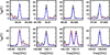Fig. 3

Transitions listed in Table C.1 and used to fit the v = 0 state of formamide (HC(O)NH₂). The blue curve represents the best LTE fit obtained with MADCUBA (Table 1). The red curve shows the simulated spectrum taking into account all the species identified so far in the region.

3.1.2 Formamide (HC(O)NH₂)

Figures 3 and 4 show the non-contaminated transitions used to fit HC(O)NH₂ and H¹³C(O)NH₂, while Fig. 5 shows the non-contaminated transitions of the vibrationally excited state v₁₂ = 1. The best-fitparameters obtained with MADCUBA for the ground state are T_ex = 150 ± 26 K, FWHM = 8.6 ± 0.2 km s⁻¹, N = (5.4 ± 1.1) ×10¹⁶ cm⁻², and X = (5.4 ± 1.5) × 10⁻⁹ (Table 1). For its ¹³C-isotopologue, H¹³C(O)NH₂, we have fixed the FWHM, the T_ex, and the v_LSR as those estimated for HC(O)NH₂ and found N = (4.7 ± 0.7) × 10¹⁵ cm⁻² and X = (4.7 ± 1.1) × 10⁻¹⁰.

From the fit results we have derived a ¹²C/¹³C ratio of 12 ± 3. As in the case of HNCO, this low ¹²C/¹³C ratio is probably affected by opacity effects. As already done for HNCO, we discuss the column density and abundance of HC(O)NH₂ assuming the ¹²C/¹³C ratio from the galactocentric distance dependence and deriving the values from those of the ¹³C-isotopologue. Thus, the corrected column density is N = (1.7 ± 0.6) × 10¹⁷ cm⁻², and the corrected abundance is X = (1.7 ± 0.7) × 10⁻⁸. These values will be used for the discussion presented in Sect. 4.

The best-fit parameters obtained with MADCUBA for the v₁₂ = 1 state are T_ex = 245 ± 88 K (consistent within the error with that obtained for v = 0), FWHM = 8.4 ± 0.2 km s⁻¹, N = (1.5 ± 0.2) × 10¹⁷ cm⁻², and X = (1.5 ± 0.4) × 10⁻⁸. Note that the column density and the abundance derived from the ¹³C-isotopologue multiplied by the ¹²C/¹³C ratio, are consistent, within the errors, with those derived separately from the HC(O)NH₂ v₁₂ = 1 state (see Table 1). This result is also consistent with what was found for HNCO, HN¹³CO, and the tentatively detected vibrationally excited states. It should be noted that if we fix T_ex of H¹³C(O)NH₂ to that obtained for the HC(O)NH₂ v₁₂ = 1 state (245 K), we obtain N = (9.1 ± 1.4) × 10¹⁵ cm⁻². Thus, the N corrected for the ¹²C/¹³C ratio would be N = (3.4 ± 1.2) × 10¹⁷ cm⁻², a factor of two higher with respect to the result obtained for the v₁₂ = 1 state of the main species, but consistent within the errors.

Since we have found that rotational transitions of the vibrationally excited state are optically thin, this could be an indication that the v = 0 state is affected by opacity effects, and that the assumed ¹²C/¹³C ratio to obtain the final results is a good approximation. In fact, if we simulate the spectrum of the transitions in Fig. 3 of HC(O)NH₂, v = 0 with the column density derived from the ¹³C-isotopologue (N = 1.7 × 10¹⁷ cm⁻²), the derived line opacities are in the range 0.3–1.1.

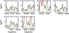Fig. 4

Transitions listed in Table C.1 and used to fit the v = 0 state of the ¹³C-isotopologue of formamide (H¹³C(O)NH₂). The dark green curve represents the best LTE fit obtained with MADCUBA (Table 1). The red curve shows the simulated spectrum taking into account all the species identified so far in the region.

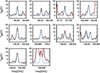Fig. 5

Transitions listed in Table C.1 and used to fit the v₁₂ = 1 state of formamide (HC(O)NH₂). The steel blue curve represents the best LTE fits obtained with MADCUBA (Table 1). The red curve shows the simulated spectrum taking into account all the species identified so far in the region.

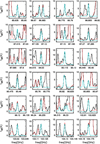Fig. 6

Transitions listed in Table C.1 and used to fit the v_b = 0 state of methyl isocyanate (CH₃NCO). The dark turquoise curve represents the best LTE fit obtained with MADCUBA (Table 1). The red curve shows the simulated spectrum taking into account all the species identified so far in the region.

3.1.3 Methyl isocyanate (CH₃NCO)

Figure 6 shows the non-contaminated transitions used to fit the ground vibrational state of CH₃NCO. The best-fit parameters obtained with MADCUBA are T_ex = 122 ± 7 K, FWHM = 7.15 ± 0.15 km s⁻¹, N = (4.3 ± 0.6) × 10¹⁶ cm⁻², and X = (4.3 ± 1.0) × 10⁻⁹.

Figure 7 shows the non-contaminated transitions for the vibrationally excited state v_b = 1. The best fithas been obtained fixing the same FWHM as the ground state, and resulted in T_ex = 91 ± 37 K, N = (1.2 ± 0.3) × 10¹⁷ cm⁻², and X = (1.2 ± 0.4) × 10⁻⁸.

One ¹³C-isotopologue, ¹³CH₃NCO, is tentatively detected because most of the transitions are contaminated or partially blended with those of other molecular species. Figure D.4 shows the less contaminated transitions of ¹³CH₃NCO, v_b = 0. In particular, the main contaminants are ³³SO₂ at 93.070 GHz, 93.071 GHz, and 93.073 GHz, CH₃NHCHO at 93.406 GHz, CH₃C(O)NH₂ at 93.459 GHz, CH₃OCHO at 93.457 GHz, CH₃COOH at 100.203 GHz, and 100.942 GHz, CH₃CHO at 101.892 GHz, and CH₃O¹³CHO at 108.576 GHz. Moreover, at 108.406 GHz the baseline derived from STATCONT is slightly high, and the simulated spectra do not match exactly the observed one. However, the peak of the simulated transition is of ~1 K and it is consistent with the error on the derived baseline (see Appendix A). To perform the final fit we have fixed the FWHM, the T_ex, and the v_LSR as those of the ground state of CH₃NCO (Sect. 3.1.3). The best fit gave as N = (4.9 ± 0.9) × 10¹⁵ cm⁻² and X = (4.9 ± 1.3) × 10⁻¹⁰. Conversely, CH₃N¹³CO was not detected and only an upper limit, consistent with what is obtained for ¹³CH₃NCO, can be provided for the column density and abundance (Table 1). As with HNCO, v₆ = 1, it was not possible to directly derive the upper limit of the CH₃N¹³CO column density due to the blending with other species, and we roughly estimated the column density by assuming the same T_ex, v_LSR, and FWHM of the ground state of CH₃NCO.

For this molecular species, the ground vibrational state has τ up to 0.12, while the v_b = 1 is optically thin (τ ≤ 0.05). Moreover, from the tentative detection of ¹³CH₃NCO, and correcting for the same ¹²C/¹³C used above, we obtain N = (1.8 ± 0.7) × 10¹⁷ cm⁻², and X = (1.8 ± 0.8) × 10⁻⁸, consistent with the results obtained for the v_b = 1 state, as already found for HNCO and HC(O)NH₂. If we simulate the spectrum of the transitions in Fig. 6 of CH₃NCO, v_b = 0 with the column density obtained from the v_b = 1 states, the derived line opacities are up to 0.4confirming that CH₃NCO, v_b = 0 is partially optically thick. Thus, we discuss the results obtained for CH₃NCO taking into accountthe best fit of the vibrationally excited state (Sect. 4).

The molecule that presents the lowest T_ex with respect to the other species studied in this work is CH₃NCO (Table 1). First of all, the T_ex found for the ground vibrational state could be affected by the opacity of these rotational transitions. Secondly, the transitions of the v_b = 1 state, from which we take the final result, present a very small range of E_up (from 285 K up 350 K). This means that the T_ex could not be well constrained. However, even considering a higher T_ex of 300 K, the derived N varies only by a factor of 1.2, consistent within the errors with the N derived leaving T_ex free.

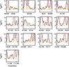Fig. 7

Transitions listed in Table C.1 and used to fit the v_b = 1 state of methyl isocyanate (CH₃NCO). The light orange curve represents the best LTE fits obtained with MADCUBA (Table 1). The red curve shows the simulated spectrum taking into account all the species identified so far in the region.

3.1.4 Acetamide (CH₃C(O)NH₂)

Figure 8 shows the non-contaminated or slightly contaminated transitions used to fit CH₃C(O)NH₂. This is the first time that CH₃C(O)NH₂ is detected towards this source. In this case, both the ground vibrational state and the excited ones (v_t = 1, 2) are optically thin (τ < 0.01), and the range of upper energies of the levels is similar for the three vibrational states (E_up from ~50 up to 250 K, see Table C.1). Moreover, since all the vibrational levels are optically thin, we have been able to fit them simultaneously with a single LTE fit. The best-fit parameters obtained with MADCUBA are T_ex = 285 ± 50 K, FWHM = 6.2 ± 0.4 km s⁻¹, N = (8 ± 4) × 10¹⁶ cm⁻², and X = (8 ± 4) × 10⁻⁹.

3.1.5 N-methylformamide (CH₃NHCHO)

Figure 9 shows the non-contaminated and slightly contaminated transitions used to fit the ground vibrational state of CH₃NHCHO. Only the transition at 102.434 GHzis slightly contaminated (~50% of contamination) with ethylene glycol at the same frequency. This is the first time that CH₃NHCHO is detected towards this source.

To fit this molecule we have fixed T_ex to 285 K (same value as for its isomer CH₃C(O)NH₂), v_LSR to 96.5 km s⁻¹, and FWHM to 7 km s⁻¹, because the fit did not converge leaving them free. The best fit of the column density obtained with MADCUBA gives N = (3.7 ± 1.6) × 10¹⁶ cm⁻², and X = (3.7 ± 1.7) × 10⁻⁹. In this case, the vibrationally excited states were not detected and upper limits to their column densities and abundances are provided (Table 1). In particular, the column density upper limits have been derived like for HNCO v₆ = 1, assuming the same T_ex, v_LSR, and FWHM of CH₃C(O)NH₂, and increasing N until the observed spectrum could be reproduced. The derived upper limits are consistent with the column density found for the ground state, within the errors.

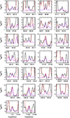Fig. 8

Transitions listed in Table C.1 and used to fit the v = 0, and v_t = 1, 2 states of acetamide (CH₃C(O)NH₂). The purple curve represents the best LTE fit obtained with MADCUBA (Table 1). The red curve shows the simulated spectrum taking into account all the species identified so far in the region.

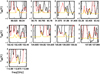Fig. 9

Transitions listed in Table C.1 and used to fit the v = 0 state of N-methylformamide (CH₃NHCHO). The gold curve represents the best LTE fit obtained with MADCUBA (Table 1). The red curve shows the simulated spectrum taking into account all the species identified so far in the region.

3.1.6 Non detections

Unlike for the other species, no unblended transitions of CH₃CH₂NCO, NH₂C(O)NH₂, NH₂C(O)CN, and HOCH₂C(O)NH₂ were found. Thus, we have derived upper limits for the column densities of the ground vibrational state. All of the transitions of these molecules are contaminated with those of other species, making it difficult to derive upper limits for the column densities. Thus, for CH₃CH₂NCO we have assumed T_ex, v_LSR, and FWHM derived for CH₃NCO v_b = 1 (since the ground state is optically thick, see Sect. 3.1.3), and have increased N to the maximum value compatible with the observed spectrum. We have obtained N ≤ 5 × 10¹⁵ cm⁻², and a molecular abundance X ≤ 5 × 10⁻¹⁰. This gives a CH₃NCO/CH₃CH₂NCO ratio >24, which is consistent with the CH₃NCO/CH₃CH₂NCO ratio >10 found towards the HMCs Orion KL and Sgr B2 by Kolesniková et al. (2018). Moreover, for NH₂C(O)NH₂, NH₂C(O)CN, and HOCH₂C(O)NH₂ we have assumed T_ex = 150 K, v_LSR = 96.5 km s⁻¹, and FWHM = 7 km s⁻¹. Also in this case we have increased N to the maximum value compatible with the observed spectrum, and found N ≤ 1.6 × 10¹⁴ cm⁻² for NH₂C(O)NH₂, N ≤ 3 × 10¹⁵ cm⁻² for NH₂C(O)CN, and N ≤ 7 × 10¹⁴ cm⁻² for HOCH₂C(O)NH₂.

3.2 Integrated intensity maps

Figure 10 shows the 1.′′2 resolution integrated intensity maps of the 3mm GUAPOS survey of the most unblended transitions of HNCO, HC(O)NH₂, CH₃NCO, CH₃C(O)NH₂, and CH₃NHCHO, with different values of theupper energy level (E_up). The velocity range used for the integrated intensity maps goes from 93 to 100 km s⁻¹. CH₃CH₂NCO, NH₂C(O)NH₂, NH₂C(O)CN, and HOCH₂C(O)NH₂ are not includedin the figure because they were not detected, as explained in Sect. 3.1.6. The transitions of HNCO overlap with those of HN¹³CO, and therefore both species contribute to the integrated emission maps.

These integrated intensity maps have been obtained from the final cubes after the calibration carried out with the CASA⁵ (Common Astronomy Software Applications) package (McMullin et al. 2007). In particular, for each transitions we have cropped the cube to frequencies ± 20 MHz around the rest frequency. Then, in the GUAPOS spectrum we have identified the channels in which the line intensity is zero and we have used these spectral windows to subtract the continuum pixel by pixel. Finally, we obtained the integrated intensity maps from the four channels around the rest frequencies. In fact, taking into account the spectral resolution of ~0.48 MHz, the width of four channels at ~90 GHz corresponds to 6.5 km s⁻¹, comparable to the FWHM of the molecular lines in this source. All these operations were made with the MADCUBA software.

The emission of the molecular species studied here arises entirely from the HMC, and comes from a region of ~2′′ (~7500 au, see Fig. 10). Moreover, the derivation of column densities from transitions at different energies is reasonable when their emission comes from the same region. Thus, we have compared the emission of the different molecules and of different range of energies for the transitions studied in this work. Figure 11 shows the comparison between the emitting region of different upper energy levels of the same molecule taken from maps of Fig. 10. Moreover, Fig. 12 shows the comparison among transitions with similar upper energy levels of different molecular species. From these figures it is clear that the emission of different transitions arises from the same region regardless of the molecule and of the upper energy level. Furthermore, we found a similar result when comparing different molecules. Only N-methylformamide (CH₃NHCHO) presents some shifts that are not significant since they are smaller than the beam size of 1.′′ 2. Thus, we can conclude that the column densities derived from transitions at different upper energy levels and the ratios derived between molecules are not affected by a different spatial distribution of different transitions or molecules.

Note, however, that this similar spatial distribution could be in part due to the fact that the emission is only partially resolved at an angular resolution of1.′′2. Therefore, to test this and eventually unveil spatial differences unresolved at 1.′′ 2 resolution, we have also analysed higher angular resolution (0.′′2) data at 1.4 mm obtained with ALMA. Figure 13 shows the integrated emission maps of the ground vibrational state $J_{K_{a}, K_{c}}$ $J_{K_{\textrm{a}},K_{\textrm{c}}}$ = 10_1,9–9_1,8 rotational transition of HC(O)NH₂, of the ground vibrational state $J_{K_{a}, K_{c}}$ $J_{K_{\textrm{a}},K_{\textrm{c}}}$ = 10_3,8–9_3,7, 10_3,7–9_3,6⁶, and 10_1,9–9_1,8 rotational transitions of HNCO, and of the ground vibrational state $J_{K_{a}, K_{c}, m}$ $J_{K_{\textrm{a}},K_{\textrm{c}},m}$ = 25_2,23,0–24_2,22,0 and the J_K,m = 25_−3,1–24_−3,1 rotational transitions of CH₃NCO. The map of the latter molecule was obtained by combining two transitions because they emit at similar frequencies and have a similar upper energy level of about 160–200 K. Note that the E_up chosen for each of these transitions was comparable to that used for the analysis and the results of the 1.′′ 2 resolution data. Moreover, we have also selected a higher E_up transition of HNCO (432 K) to show possible spatial differences. In this case, despite the different E_up of the two HNCO levels (101 K and 432 K), both transitions fill the beam of the GUAPOS observations (bottom panels of Fig. 13).

We did not find strong and unblended transitions of CH₃C(O)NH₂ and CH₃NHCHO in the narrow spectral bands of the high-angular resolution observations at 1.4 mm. Thus, these two molecules will not be discussed in the following of this section.

The 0.′′2 resolution integrated intensity maps show that the overall behaviour at 1.4 mm of these molecules (HNCO, HC(O)NH₂, and CH₃NCO) is quite similar. One of the main differences is that the maps at higher E_up (159–201 K, and 432 K, of CH₃NCO and HNCO, respectively) present a more compact structure than the lower energy ones (61 and 101 K, of HC(O)NH₂ and HNCO, respectively). This is expected because of the temperature gradient present towards the HMC, with higher temperatures to the centre with respect to the outer part as already discussed in Sect. 2.3. A striking feature of the integrated emission at high angular resolution is its ring-like morphology. This spatial distribution is similar to that traced by other COMs, such as CH₃CN and CH₃OCHO, observed with the same angular resolution of 0.′′2 (Beltrán et al. 2018). The explanation for this morphology is that most of the emission comes from a rotating and infalling toroid surrounding a small protocluster of 4 massive protostars (indicated as black squares and named A, B, C, and D in Fig. 13, see also Beltrán et al. 2021). Since the material is flowing inwards and locally the continuum temperature is higher than the T_ex of the molecules, the gas is seen in red-shifted absorption towards the centre (see Beltrán et al. 2018 for more details), and the integrated emission shows this characteristic ring structure.

The high-angular resolution maps at 1.4 mm show that the molecular emission arise from the whole HMC, filling the 1.′′ 2 beam of GUAPOS (black dashed line in Fig. 13). The column densities obtained from a region of 1.′′ 2 in the high-angular resolution maps are consistent to those derived from the GUAPOS data. In fact, if we fix T_ex, v_LSR and FWHM to the values derived at 3 mm (Table 1), the column densities of the three molecules obtained at 1.4 mm are consistent within a factor of 2 with those obtained at 3 mm. In particular, from 1.4 mm observations, N(HC(O)NH₂) = (2.5 ± 1.9) × 10¹⁶ cm⁻², N(HNCO) = (1.12 ± 0.04) × 10¹⁷ cm⁻², N(HNCO) = (9.1 ± 1.8) × 10¹⁶ cm⁻², from the transitions at 219.656 and 219.656 GHz, respectively, and N(CH₃NCO) = (6.9 ± 1.8) × 10¹⁶ cm⁻². This mean that both observations (at 1.4 and 3 mm), despite of the different angular resolution, are sensitive to approximately the same gas.

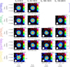Fig. 10

ALMA 1.′′2 resolution integrated emission maps at 3 mm of transitions with different E_up (from 0 up to 200 K, different columns) of HC(O)NH₂, HNCO, CH₃NCO, CH₃C(O)NH₂, and CH₃NHCHO (different rows) obtained with the GUAPOS survey. In each panel, the white contours show the continuum emission levels at 5, 10, 20, 40, 60, 100, and 200 times the rms value of 0.8 mJy beam⁻¹. The white ellipse in the lower left corner represents the synthesised beam.

Fig. 11

Maps of the integrated emission for the molecules studied in this paper. Different colours within the same panel represent the range of upper energy levels of the transitions taken into account. The contours represents 0.5 times the integrated emission peak level of the corresponding map. The beam is indicated in the left-bottom corner of the maps.

Fig. 12

Maps of the integrated emission for the molecules studied in this paper. Different colours within the same panel represent different molecules. The contours represents 0.5 times the integrated emission peak level of the corresponding map. The beam is indicated in the left-bottom corner of the maps.

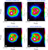Fig. 13

ALMA 0.′′2 resolution integrated emission maps at 1.4 mm of HC(O)NH₂ (10_1,9–9_1,8) (top-left panel), CH₃NCO (25_2,23,0–24_2,22,0 and 25_−3,−,1–24_−3,−,1) (top-right panel), HNCO (10_3,8–9_3,7 and 10_3,7–9_3,6) (bottom-left panel), and HNCO (10_1,9–9_1,8) (bottom-right panel) in a velocity range between 93 and 100 km s⁻¹ for each transition. The contour levels are 0.3, 0.4, 0.5, 0.6, 0.7, 0.8, and 0.9 the maximum value of the maps. The maximum values of the maps are 1.625 Jy beam⁻¹ km s⁻¹ for HC(O)NH₂, 0.877 Jy beam⁻¹ km s⁻¹for CH₃NCO, 1.082 Jy beam⁻¹ km s⁻¹ for HNCO at219.656 GHz, and 1.396 Jy beam⁻¹ km s⁻¹ for HNCO at 220.585 GHz. The black dashed circle indicates in all the panels the area in which the spectrum analysed in this work was extracted, which matches the GUAPOS beam of 1.′′ 2 centered at the 3mm continuum peak. The frequency and E_up energies of the transitions are shown in blue above each panel, and in red in the top-right corner of each panel, respectively.The synthesised beam is represented by the grey ellipse in the lower left corner. The black squares indicates the position of the continuum sources A, B, C, and D resolved with 7 mm VLA observations by Beltrán et al. (2021).

4 Discussion

To obtain a complete overview of the chemical processes that lead to the formation of peptide-like bond molecules in the ISM, we have compared the results obtained in G31 with those in other interstellar sources. Comparisons have been made with works containing at least the detection of HC(O)NH₂ together with that of CH₃NCO and/or CH₃C(O)NH₂. These sources are the HMCs in the GC Sgr B2(N) (Belloche et al. 2013), Sgr B2(N2) (Belloche et al. 2017), Sgr B2(N1S) (Belloche et al. 2019), Sgr B2(N3) and Sgr B2(N5) (Bonfand et al. 2019), the HMCs in the Galactic disk G10.47+0.03 (hereafter G10.47), Orion BN/KL A and B, and NGC 6334I (Gorai et al. 2020; Cernicharo et al. 2016; Ligterink et al. 2020, respectively), the hot core precursor G328.2551-0.5321 (hereafter G328.2551) A, B (related to accretion shock positions), and envelope (hereafter env) positions (Csengeri et al. 2019), the hot corinos IRAS 16293-2422 (hereafter IRAS 16293) A and B (Martín-Doménech et al. 2017; Ligterink et al. 2017, 2018; Manigand et al. 2020), and the GC molecular cloud G+0.693-0.027 (hereafter G+0.693, Zeng et al. 2018). The Sgr B2(N) and G+0.693 observations were taken with different single-dish telescope (IRAM 30m and Green Bank Telescope) while the rest were observed using ALMA. Moreover, we have also compared the column densities with those of HNCO and HC(O)NH₂ and the upper limits of CH₃NCO and CH₃C(O)NH₂ estimated in the comet 67P/Churyumov-Gerasimenko (hereafter 67P) by the ROSINA experiment on ESA’s Rosetta mission reported by Altwegg et al. (2017).

4.1 Molecular abundances

Six of the works listed above provide an estimate of N(H₂) and make it possible to compare with the molecular abundances obtained in this work. Figure 14 shows the molecular abundances derived in G31 and in the other regions. For abundances whose errors were not provided we assumed a value of 25%. We note however that the N(H₂) used for IRAS 16293 B should be considered as a lower limit since dust might be optically thick (e.g. Jørgensen et al. 2016, and thus the abundances for this source should be taken as upper limits. At a glance, we can see that G31, in addition to Sgr B2(N2), is the only other source in which all of the five molecules (HNCO, HC(O)NH₂, CH₃NCO, CH₃C(O)NH₂, and CH₃NHCHO) have been detected. The behaviour of these two HMCs looks similar, except for HC(O)NH₂, which showsan over-abundance towards Sgr B2(N2). In most of the sources HNCO is the most abundant species, followed by HC(O)NH₂, CH₃NCO, CH₃C(O)NH₂, and CH₃NHCHO. The only exceptions are IRAS 16293 B and Sgr B2(N2), whose HNCO and HC(O)NH₂ abundances are similar between them, and G10.47, for which CH₃NCO is more abundant than HC(O)NH₂. Moreover, both HNCO and HC(O)NH₂ abundances towards G31 are comparable with those of the GC molecular cloud G+0.693 (Zeng et al. 2018). HC(O)NH₂ and CH₃NCO abundances together are similar to those derived towards the HMCs G10.47 and Sgr B2(N5), and the HMC precursor G328.2551 (Gorai et al. 2020; Bonfand et al. 2019; Csengeri et al. 2019), while only the HC(O)NH₂ abundance is similar tothat of the low-mass protostar IRAS 16293 B (Martín-Doménech et al. 2017). All these similarities are within a factor of 4, and should be taken with caution since possible opacity effects of HNCO and HC(O)NH₂ might have affected the derived abundances towards some of these sources (see Sect. 3). For G31 this is not the case since column densities, and thus abundances, have been derived from the ¹³C-isotopologues or the vibrationally excited states, which are optically thin (see Table C.1).

The high molecular abundances found in HMCs, hot corinos, and G+0.693 (10⁻¹⁰–10⁻⁶) are consistent with their formation through pathways on the surface of dust grains at earlier phases, and subsequent desorption, induced by thermal heating (for HMCs and hot corinos) or by grain sputtering produced by shocks (for G+0.693 and the accretion shocks G328.2551 A and B, Zeng et al. 2020; Csengeri et al. 2019). In fact, in absence of efficient desorption mechanisms, the gas-phase abundances are expected to be lower, as occurs in low-mass pre-stellar cores such as L1544 where the upper limits for the abundances of HC(O)NH₂ and CH₃NCO that have been reported are very low (X(HC(O)NH₂) < 8.7 × 10⁻¹³ and X(CH₃NCO) < 4.2 × 10⁻¹¹, Jiménez-Serra et al. 2016).

Figure 15 shows the comparison between pairs of molecular abundances, HC(O)NH₂ and HNCO, CH₃NCO and HNCO, and CH₃NCO and HC(O)NH₂. It is already known from previous observations that there is a correlation between HNCO and HC(O)NH₂ (López-Sepulcre et al. 2015, 2019; Allen et al. 2020). In the top-left panel of Fig. 15 the best power-law fits derived by López-Sepulcre et al. (2015), X[HC(O)NH₂] = 0.04 × X[HNCO]^0.93, and by Quénard et al. (2018), X[HC(O)NH₂] = 32.14 × X[HNCO]^1.29, are compared with the one derived here, X[HC(O)NH₂] = 0.006 × X[HNCO]^0.73 (with a Pearson coefficient of 0.99 and a P-value <0.05, indicating a strong positive correlation). Thus, the sample of sources discussed in this work, which also includes HMCs and a shock-dominated molecular cloud, is in agreement with the correlation found previously for low- and intermediate-mass pre-stellar and protostellar objects, which holds across several orders of magnitude in abundance. Based on this tight correlation, it has been proposed that the two species are chemically related and that the formation of HC(O)NH₂ might occur through H-addition to solid-phase HNCO (e.g. Tielens & Hagen 1982; Charnley et al. 2004). Experimental works first suggested that this process is not efficient (Noble et al. 2015; Fedoseev et al. 2015), while recent works revised this possibility and found that a correlation between these two molecular species can be understood by H-abstraction and addition reactions (e.g. Nguyen et al. 2011; Haupa et al. 2019; Suhasaria & Mennella 2020). Moreover, hydrogenation of NO combined with UV-photon exposure and radical-radical reactions on grains has been suggested as the main formation pathways for both HNCO and HC(O)NH₂ (e.g. Jones et al. 2011; Fedoseev et al. 2016; Ligterink et al. 2018; Dulieu et al. 2019). Coutens et al. (2016) found that the deuteration (D/H ratio) of HC(O)NH₂ in IRAS 16293 B is similar to that of HNCO, in agreement with the hypothesis that both species are chemically related via grain-surface reactions. Gas-phase formation routes have also been proposed (see e.g. NH₂ + H₂CO, Barone et al. 2015; Skouteris et al. 2017). Laboratory experiments by Martín-Doménech et al. (2020) show that both HNCO and HC(O)NH₂ could form upon UV photoprocessing or electron irradiation of ice samples, indicating that energetic processing (like UV photons and cosmic rays) of ISM CO-rich ices could form both species, without the need of a chemical link and/or a similar precursor between the two. This was predicted by the chemical modelling of Quénard et al. (2018), who showed that the formation of HC(O)NH₂ at different temperature regimes is governed by different chemical processes. While at low temperatures the formation of HC(O)NH₂ is driven by gas-phase formation via the reaction NH₂ + H₂CO → HC(O)NH₂ + H, at high temperature its formation occurs on the surface of dust grains via radical-radical addition reactions. Moreover, they showed that for HNCO grain-surface and gas-phase reactions are equally efficient at low temperature, while at high temperatures the gas-phase formation predominates and the small fraction formed on grains is released into the gas phase via thermal desorption. Rimola et al. (2018) also showed via theoretical quantum chemical computations that HC(O)NH₂ can form on grain surfaces starting from CN, which can quickly react with water-rich amorphous ices. Thus, the correlation between HNCO and HC(O)NH₂ is mainly due to a similar response to the temperature of the two molecules, and not to a direct chemical link. In fact, the increase of the temperaturetriggers processes on the ice-mantle of grains, such as thermal evaporation. Moreover, as discussed above, other processes, like UV photons, cosmic rays, and shocks, could help both on the formation of these molecules on grain surfaces and on their desorption in the gas.

Similar to the HNCO vs. HC(O)NH₂ relation, we have found similar correlations (Fig. 15) between CH₃NCO and HNCO, X[CH₃NCO] = 0.0015 × X[HNCO]^0.73, and betweenCH₃NCO and HC(O)NH₂, X[CH₃NCO] = 0.02 × X[HC(O)NH₂]^0.84 (both with a Pearson coefficient of 0.99 and a P-value <0.05, indicating strong positive correlations), suggesting links also between CH₃NCO and HNCO, and HC(O)NH₂. A correlation between CH₃NCO and HNCO was already suggested by Ligterink et al. (2021), who found that the CH₃NCO and HNCO column density ratio is almost constant in different regions. It was proposed by Halfen et al. (2015) that CH₃NCO could form in gas phase through HNCO from the reaction: $HNCO + {CH}_{3} \to {CH}_{3} NCO + H,$ $\begin{equation*}\textrm{HNCO} + \textrm{CH}_{3} \rightarrow \textrm{CH}_{3}\textrm{NCO} + \textrm{H}, \end{equation*}$ (1)

or from $\begin{array}{l} HNCO + {CH}_{5}^{+} \to {CH}_{3} {NCOH}^{+} + H_{2} \\ {CH}_{3} {NCOH}^{+} + e^{-} \to {CH}_{3} NCO + H . \end{array}$ $\begin{align*} &\textrm{HNCO} + \textrm{CH}_{5}^{+} \rightarrow {\textrm{CH}}_{3}\textrm{NCOH}^{+} + \textrm{H}_{2} \\ &\textrm{CH}_{3}\textrm{NCOH}^{+} + \textrm{e}^{-} \rightarrow \textrm{CH}_{3}\textrm{NCO} + \textrm{H}. \end{align*}$

Cernicharo et al. (2016) found a similar spatial distribution for HNCO, HC(O)NH₂ and CH₃NCO towards Orion BN/KL, as observed for G31 in this work (Fig. 13), and suggested reaction (1) as a possible grain-surface reaction to form CH₃NCO. Moreover, the HNCO/CH₃NCO abundance ratio found for G31 of 12 ± 6 is consistent with the range of values predicted by the HMC model of Belloche et al. (2017), who proposed CH₃NCO grain-surface formation and ice sublimation during the warm-up phase (e.g. through thermal desorption as suggested for HNCO and HC(O)NH₂). Formation of CH₃NCO through HNCO and methane has also been considered on ices, where favourable thermodynamic conditions could be created (e.g. reduction of the energy barrier, Cassone et al. 2021). More recently Majumdar et al. (2018) found that reaction (1) is endothermic, and they proposed alternative routes for the formation of methyl-isocyanate on grains: $\begin{array}{l} {CH}_{3} + OCN \to {CH}_{3} NCO, \\ N + {CH}_{3} CO \to {CH}_{3} C (N) O \to {CH}_{3} NCO, \end{array}$ $\begin{align*} \label{} &\textrm{CH}_{3} + \textrm{OCN} \rightarrow \textrm{CH}_{3}\textrm{NCO},\\ &\textrm{N} + \textrm{CH}_{3}\textrm{CO} \rightarrow {\textrm{CH}}_{3}\textrm{C(N)O} \rightarrow \textrm{CH}_{3}\textrm{NCO}, \end{align*}$

or through the HCN⋯ CO van der Waals complex $\begin{array}{l} H + HCN \dots CO \to H_{2} CN \dots CO \to H_{2} CNCO \\ H + H_{2} CNCO \to {CH}_{3} NCO . \end{array}$ $\begin{align*} \label{} &\textrm{H} + \textrm{HCN} \cdots {\textrm{CO}} \rightarrow {\textrm{H}}_{2}\textrm{CN} \cdots {\textrm{CO}} \rightarrow {\textrm{H}}_{2}\textrm{CNCO} \\ &\textrm{H} + \textrm{H}_{2}\textrm{CNCO} \rightarrow \textrm{CH}_{3}\textrm{NCO}. \end{align*}$

Interestingly a similar process has also been found to be important for the formation of HNCO: $N \dots CO + H \to HNCO,$ $\begin{equation*} \label{} \textrm{N} \cdots {\textrm{CO}} + \textrm{H} \rightarrow {\textrm{HNCO}}, \end{equation*}$ (8)

indicating that a possible link between the two species could be the van der Waals complexes involving CO. Finally, the correlation between CH₃NCO and HC(O)NH₂ (bottom panel of Fig. 15) is probably due to the fact that both molecules form on grains and are desorbed on gas phase because of similar physical effects. For example, both molecules are expected to be already efficiently thermally desorbed at the high temperatures of HMCs (>100 K). In fact, temperature-programmed desorption experiments show that the HC(O)NH₂ peak desorption temperature is around 200 K (Ligterink et al. 2018), while that of CH₃NCO is around 150 K (Ligterink et al. 2017). Thus, we expect most of both molecules to have been already released back to the gas phase in hot cores.

Thus, a strong correlation between two molecules in a sample of sources does not directly imply that these molecules are chemically related (e.g. Belloche et al. 2020). Whether these results are a consequence of a direct chemical link or an effect caused by similar chemical responses to physical conditions cannot be firmly concluded yet, and more dedicated physico-chemical models are needed to disentangle all of the possible effects.

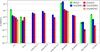Fig. 14

Molecular abundances (X) with respect to H₂ towards G31, G10.47, G328.2551 A, B, and env, Sgr B2(N2), Sgr B2(N5), IRAS 16293 B (upper limits), and G+0.693. Different colours represent the different molecules for which the abundances are shown, as indicated in the legend in the upper-right corner. Data are taken from: G31 (this work), G10.47 (Gorai et al. 2020), G328.2551 (Csengeri et al. 2019), Sgr B2(N2) (Belloche et al. 2017), Sgr B2(N5) (Bonfand et al. 2019), IRAS 16293 B (Martín-Doménech et al. 2017), and G+0.693 (Zeng et al. 2018) (from the left to the right).

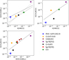Fig. 15

Upper-left panel: X[HC(O)NH₂] as a functionof X[HNCO]. The solid line is the power-law fit obtained in this work, while the dashed and pointed lines are those obtained by López-Sepulcre et al. (2015) and Quénard et al. (2018), respectively. Upper-right panel: X[CH₃NCO] as a functionof X[HNCO]. The solid line is the power-law fit obtained in this work. Lower panel: X[CH₃NCO] as a functionof X[HC(O)NH₂]. The solid line is the power-law fit obtained in this work. In all the panels, the different colours represent the different sources, as indicated in the bottom-right legend. Data are taken from the same works indicated in Fig. 14.

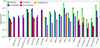Fig. 16

Molecular abundances with respect to CH₃OH towards G31, G328.2551 A, B, and env, Sgr B2(N), Sgr B2(N2), Sgr B2(N3), Sgr B2(N5), NGC 6334I MM1-i–v and MM2-i–ii, Orion BN/KL A and B, IRAS 16293 A and B, and G+0.693. Different colours represent the different molecules for which the abundances are shown, as indicated in the legend in the upper-left corner. Data are taken from: G31 (this work, Mininni et al. in prep.), G328.2551 (Csengeri et al. 2019), Sgr B2(N) (Belloche et al. 2013), Sgr B2(N2) (Belloche et al. 2016, 2017), Sgr B2(N3) and Sgr B2(N5) (Bonfand et al. 2019), NGC 6334I (Bøgelund et al. 2018; Ligterink et al. 2020), Orion BN/KL A and B (Cernicharo et al. 2016), IRAS 16293 A (Ligterink et al. 2017; Manigand et al. 2020), IRAS 16293 B (Ligterink et al. 2017, 2018; Jørgensen et al. 2018), and G+0.693 (Zeng et al. 2018; Rodríguez-Almeida et al. 2021) (from the left to the right).

4.2 Abundances with respect to CH₃OH

In this section, we have performed an analysis similar to that shown in Sect. 4.1 comparing the abundances derived with respect to methanol, CH₃OH. All the sources are included, except Sgr B2 (N1S) for which the CH₃OH column density is not found in the literature, and G10.47 for which whose CH₃OH column density has been derived from Submillimeter Array observations (Rolffs et al. 2011) and not from ALMA observations as for the rest of the sources. Thus, these two sources are excluded from the discussion in this section. Moreover, for G31, G+0.693, Sgr B2(N), NGC 6334I, and IRAS 16293 A and B, N(CH₃OH) has been derived from the optically thin isotopologues ¹³CH₃OH (for G31, Mininni et al., in prep.) and CH $_{3}^{18}$ $_{3}^{18}$ OH (for the other sources, Rodríguez-Almeida et al. 2021; Belloche et al. 2013; Bøgelund et al. 2018; Manigand et al. 2020; Jørgensen et al. 2018), after taking into account the ¹²C/¹³C and ¹⁶O/¹⁸O ratios corrections as a function of the galactocentric distance (Yan et al. 2019 for G31; Wilson & Rood 1994 for G+0.693, Sgr B2(N), and IRAS 16293 B; Wilson 1999 for NGC 6334I and IRAS 16293 A). Conversely, N(CH₃OH) for Sgr B2(N2), Sgr B2(N3), Sgr B2(N5), Orion BN/KL and G328.2551 has been obtained from the main isotopologue and could be affected by line opacity effects (Belloche et al. 2016; Bonfand et al. 2019; Cernicharo et al. 2016; Csengeri et al. 2019).

Figure 16 shows the abundances with respect to CH₃OH (N/N(CH₃OH)). First of all, G328.2551 and Sgr B2(N3) present similar N/N(CH₃OH) for HC(O)NH₂ and CH₃NCO with respect to G31, and Sgr B2(N2) presents similar N/N(CH₃OH) for all the molecules except for HC(O)NH₂. Except for HNCO, Sgr B2(N) and Sgr B2(N5) present higher column density ratios than G31 with respect to CH₃OH. Moreover, NGC 6334I has similar N/N(CH₃OH) with respect to G31 towards all the positions, except for MM1-v for which higher ratios have been found for HNCO, HC(O)NH₂, and CH₃NHCHO. Orion BN/KL A and B have ratios similar to those of G31 for all the peptide-like bond molecular species, while IRAS 16293 A and B have lower N/N(CH₃OH) ratios. Finally, with respect to G31, G+0.693 presents higher ratios for HNCO and HC(O)NH₂, and a similar one for CH₃NCO. It should be noted that all the similarities are within a factor of 4.

The general trend is that most of the sources show similar N/N(CH₃OH) ratios, except for IRAS 16293 A and B, which present lower values, and Sgr B2(N), Sgr B2(N5), and G+0.693 that show higher values with respect to G31 and the other sources. Moreover, on average the N/N(CH₃OH) of HNCO is the highest, followed by that of HC(O)NH₂, CH₃NCO, CH₃C(O)NH₂, and CH₃NHCHO, similar to what was found for the abundances derived with respect to N(H₂).

In Fig. 17 we show the comparison between pairs of N/N(CH₃OH) ( $X_{{CH}_{3} OH}$ $X_{\textrm{CH}_{3}\textrm{OH}}$ ). In particular, the best power-law fits are: $\begin{array}{l} X_{{CH}_{3} OH} (HC (O) {NH}_{2}) = 0.18 \times X_{{CH}_{3} OH} {(HNCO)}^{0.92}, \\ X_{{CH}_{3} OH} ({CH}_{3} NCO) = 0.032 \times X_{{CH}_{3} OH} {(HNCO)}^{0.69}, \\ X_{{CH}_{3} OH} ({CH}_{3} NCO) = 0.05 \times X_{{CH}_{3} OH} {(HC (O) {NH}_{2})}^{0.48}, \\ X_{{CH}_{3} OH} ({CH}_{3} C (O) {NH}_{2}) = 0.022 \times X_{{CH}_{3} OH} {(HNCO)}^{0.74}, \\ X_{{CH}_{3} OH} ({CH}_{3} C (O) {NH}_{2}) = 0.042 \times X_{{CH}_{3} OH} {(HC (O) {NH}_{2})}^{0.69} . \end{array}$ $\begin{align*} \label{} & X_{\textrm{CH}_{3}\textrm{OH}}(\textrm{HC(O)NH}_{2})\,{=}\,0.18\,{\times}\, X_{\textrm{CH}_{3}\textrm{OH}}(\textrm{HNCO})^{0.92}, \\ & X_{\textrm{CH}_{3}\textrm{OH}}(\textrm{CH}_{3}\textrm{NCO})\,{=}\,0.032\,{\times}\, X_{\textrm{CH}_{3}\textrm{OH}}(\textrm{HNCO})^{0.69}, \\ & X_{\textrm{CH}_{3}\textrm{OH}}(\textrm{CH}_{3}\textrm{NCO})\,{=}\,0.05\,{\times}\, X_{\textrm{CH}_{3}\textrm{OH}}(\textrm{HC(O)NH}_{2})^{0.48}, \\ & X_{\textrm{CH}_{3}\textrm{OH}}(\textrm{CH}_{3}\textrm{C(O)NH}_{2})\,{=}\,0.022\,{\times}\, X_{\textrm{CH}_{3}\textrm{OH}}(\textrm{HNCO})^{0.74}, \\ & X_{\textrm{CH}_{3}\textrm{OH}}(\textrm{CH}_{3}\textrm{C(O)NH}_{2})\,{=}\, 0.042\,{\times}\, X_{\textrm{CH}_{3}\textrm{OH}}(\textrm{HC(O)NH}_{2})^{0.69}. \end{align*}$

Thus, also in this case we have found positive correlations between HC(O)NH₂ and HNCO, CH₃NCO and HNCO, and CH₃NCO and HNCO, as already discussed in Sect. 4.1. Moreover, thanks to the available data we have also found for the first time correlations between CH₃C(O)NH₂ and HNCO, and CH₃C(O)NH₂ and HC(O)NH₂.

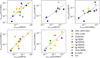Fig. 17

Upper-left panel: $X_{{CH}_{3} OH}$ $X_{\textrm{CH}_{3}\textrm{OH}}$ (HC(O)NH₂) as a functionof $X_{{CH}_{3} OH}$ $X_{\textrm{CH}_{3}\textrm{OH}}$ (HNCO). Upper-central panel: $X_{{CH}_{3} OH}$ $X_{\textrm{CH}_{3}\textrm{OH}}$ (CH₃NCO) as a functionof $X_{{CH}_{3} OH}$ $X_{\textrm{CH}_{3}\textrm{OH}}$ (HNCO). Upper-right panel: $X_{{CH}_{3} OH}$ $X_{\textrm{CH}_{3}\textrm{OH}}$ (CH₃NCO) as a functionof $X_{{CH}_{3} OH}$ $X_{\textrm{CH}_{3}\textrm{OH}}$ (HC(O)NH₂). Bottom-left panel: $X_{{CH}_{3} OH}$ $X_{\textrm{CH}_{3}\textrm{OH}}$ (CH₃C(O)NH₂) as a functionof $X_{{CH}_{3} OH}$ $X_{\textrm{CH}_{3}\textrm{OH}}$ (HNCO). Bottom-central panel: $X_{{CH}_{3} OH}$ $X_{\textrm{CH}_{3}\textrm{OH}}$ (CH₃C(O)NH₂) as a functionof $X_{{CH}_{3} OH}$ $X_{\textrm{CH}_{3}\textrm{OH}}$ (HC(O)NH₂). In all the panels, the solid lines are the power-law fit obtained in this work, and the different colours represent the different sources, as indicated in the bottom-right legend. Data are taken from the same works indicated in Fig. 16.

4.3 Column density ratios

Figure 18 shows the column density ratios of HNCO, CH₃NCO, CH₃C(O)NH₂, and CH₃NHCHO with respect to HC(O)NH₂ in the differentastronomical sources. For column densities whose errors were not provided we assumed a value of 25%. For IRAS 16293 B two values are shown, corresponding to those derived by Martín-Doménech et al. (2017), and Ligterink et al. (2017, 2018). From the left to the right, Fig. 18 shows massive and low-mass star-forming regions, the GC G+0.693 molecular cloud, and the comet 67P values.

We note that overall there are similarities between molecular abundance ratios towards different regions, typically within ~1 order of magnitude in the 80% of the sources. TheHNCO/HC(O)NH₂ ratio found in G31 is similar, within the errors, to those derived towards Orion BN/KL-A, NGC 6334I MM1-v, MM2-i, and MM2-ii, G10.47, IRAS 16293 B, and G+0.693 (top-left panel of Fig. 18). The CH₃NCO/HC(O)NH₂ ratio is consistent, within the errors, to those of Sgr B2(N), Sgr B2(N1S), IRAS 16293 B, G328.2551 B and env, and G+0.693 (top-right panel of Fig. 18). The CH₃C(O)NH₂/HC(O)NH₂ ratio is consistent, within the errors, to those of Sgr B2(N1S), Orion BN/KL-A, NGC 6334I MM1-iv, MM2-i, andMM2-ii, and IRAS 16293 B (bottom-left panel of Fig. 18). The CH₃NHCHO/HC(O)NH₂ ratio is similar, within the errors, to those of Sgr B2(N1S), NGC 6334I MM1-v, MM1-vi, MM1-vii, MM1-viii, and MM1-nmf, which are all the sources in which CH₃NHCHO has been detected, except Sgr B2(N2) (bottom-right panel of Fig. 18). The CH₃NHCHO/CH₃C(O)NH₂ ratio is overall similar in all the sources, as observed in the bottom panels of Fig. 18 where their column density ratios with respect to HC(O)NH₂ are shown.

The similarities of the different molecular ratios in interstellar regions with very different physical properties (e.g. masses from ~0.5 M_⊙ up to ~100 M_⊙ and luminosities from ~1 L_⊙ up to ~10⁷ L_⊙) and location in the Galaxy, such as high-mass and low-mass star-forming regions (HMCs and hot corinos, respectively) in the GC and in the galactic disk, and a GC molecular cloud with no signs of star formation yet (Zeng et al. 2020), suggest that these molecules were formed during very early phases of evolution. In fact, as discussed in Sect. 4.1, these species could have been formed mostly on grains, and, in a later stage, released back to gas phase through thermal desorption, in HMCs and hot corinos, or through shock-induced grain sputtering, in the case of G+0.693 and G328.2551 accretion shock positions. This has also been suggested by Coletta et al. (2020), who found constant abundance ratios for H₃OCHO, CH₃OCH₃, C₂H₅CN, and HC(O)NH₂ towards low- and high-mass star-forming regions in different evolutionary stages. For the GC, a similar conclusion was proposed by Requena-Torres et al. (2006) who compared the abundances of O-bearing COMs derived towards giant molecular clouds in the GC with those measured in hot corinos and hot cores. They found that all of these abundances are consistent within a factor of 10 and suggested that COMs are ejected from grain mantles by shocks.

Regarding the formation of CH₃C(O)NH₂, Quan & Herbst (2007) have proposed that it could be formed in gas phase via radiative association reaction, like: $\begin{array}{l} HC (O) {NH}_{2} + {CH}_{3}^{+} \to {CH}_{3} {CHONH}_{2}^{+} + h ν \\ {CH}_{3} {CHONH}_{2}^{+} + e^{-} \to {CH}_{3} C (O) {NH}_{2} + H, \end{array}$ $\begin{align} \label{} &\textrm{HC(O)NH}_{2} + \textrm{CH}_{3}^{+} \rightarrow {\textrm{CH}}_{3}\textrm{CHONH}_{2}^{+} + h\nu\\ &\textrm{CH}_{3}\textrm{CHONH}_{2}^{+} + \textrm{e}^{-} \rightarrow {\textrm{CH}}_{3}\textrm{C(O)NH}_{2} + \textrm{H},\end{align}$

Halfen et al. (2011) have suggested that ion-molecule processes might lead to the formation of both CH₃C(O)NH₂ and CH₃NHCHO, and more recently Redondo et al. (2014) have studied the viability of ion-molecule gas-phase reactions, such as CH $_{5}^{+}$ $_{5}^{+}$ + HC(O)NH₂, to form CH₃C(O)NH₂. However, only gas-phase reactions are not enough to reproduce the observed abundances and the CH₃C(O)NH₂/HC(O)NH₂ ratios in the ISM. Frigge et al. (2018) show that CH₃NHCHO could form in a mixture of methylamine (CH₃NH₂) and CO ices, upon irradiation with energetic electrons. In particular, they proposed the following reactions on grain surfaces: ${CH}_{3} {NH}_{2} + CR \to {CH}_{3} NH + H$ $\begin{align*} &\textrm{CH}_{3}\textrm{NH}_{2} + \textrm{CR} \rightarrow {\textrm{CH}}_{3}\textrm{NH} + \textrm{H} \end{align*}$ (16) ${CH}_{3} NH + HCO \to {CH}_{3} NHCHO,$ $\begin{align*} &\textrm{CH}_{3}\textrm{NH} + \textrm{HCO} \rightarrow {\textrm{CH}}_{3}\textrm{NHCHO}, \end{align*}$ (17)

where CR are the cosmic rays simulated by energetic electrons. Moreover, Garrod et al. (2008) have proposed CH₃ + HNCO as a possible formation route on grains, while Belloche et al. (2017) suggest that CH₃C(O)NH₂ is predominantly formed by H-abstraction from HC(O)NH₂, followed by methyl-group (CH₃) addition, and by the reaction NH₂ + CH₃CO. Moreover, these authors found that CH₃NHCHO could be formed on grains either through the direct addition of functional-group radicals (e.g. CH₃ + HNCHO) or through the hydrogenation of CH₃NCO. CH₃C(O)NH₂ has also been identified in carbonaceous chondrites (Cooper & Cronin 1995), and was found to form in experiments with irradiated ices (e.g. Berger 1961; Ligterink et al. 2018), favouring also the grain-surface formation.

The lower left panel of Fig. 18 shows that CH₃C(O)NH₂ is well correlated with HC(O)NH₂, as we already found from the correlation of their abundances with respect to CH₃OH (see Sect. 4.2). The CH₃C(O)NH₂/HC(O)NH₂ ratios are all within ~1 order of magnitude. This might indicate a direct chemical link, as suggested by reactions (14) and (15), or that both molecules are mainly formed on grain surface and desorb under similar physical conditions, as proposed by Quénard et al. (2018) for HNCO and HC(O)NH₂. Indeed, thishypothesis is supported by the temperature programmed desorption experiment of Ligterink et al. (2018), who have showed that the peak desorption temperatures of CH₃C(O)NH₂ and HC(O)NH₂ are very similar (219 and 210 K, respectively, see also Corazzi et al. 2020).

Finally, a comparison with the values found in the comet 67P shows that the CH₃C(O)NH₂/HC(O)NH₂ and CH₃NHCHO/HC(O)NH₂ upper limits (bottom-right panel of Fig. 18) are consistent with the values observed in the ISM, while the HNCO/HC(O)NH₂ ratio is smaller than the ISM values. This could be due to an over-abundance of HC(O)NH₂ in the 67P comet with respect to the ISM that could indicate a chemical reprocessing during later stages, such as the protoplanetary disk phase. However, the measurements with Rosina (Rosetta Orbiter Spectrometer for Ion and Neutral Analysis) cannot distinguish between the different structural isomers, so, if the other isomers were also formed, the abundance of HC(O)NH₂ would be lower.

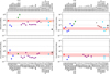Fig. 18

HNCO, CH₃NCO, CH₃C(O)NH₂, and CH₃NHCHO column density ratios with respect to HC(O)NH₂ (upper-left, upper-right, bottom-left, and bottom-right panels, respectively) towards G31 (red points and shaded areas) and high- and low-mass star-forming regions, a GC molecular cloud, and the 67P comet (from the left to the right in all panels). Different colours represent: G31 in red, Sgr B2 in blue, Orion BN/KL in green, NGC 6334I in purple, G10.47 in grey, G328.2551 in brown, IRAS 16293 in light blue, G+0.693 in orange, and the comet 67P in black. Data are taken from: G31 (this work), Sgr B2(N) (Belloche et al. 2013), Sgr B2(N2) (Belloche et al. 2017), Sgr B2(N1S) (Belloche et al. 2019), Sgr B2(N3) and Sgr B2(N5) (Bonfand et al. 2019), Orion BN/KL - A and B (Cernicharo et al. 2016), NGC 6334I MM1-i–MM2ii (Ligterink et al. 2020), G10.47 (Gorai et al. 2020), G328.2551 A, B and env (Csengeri et al. 2019), IRAS 16293 A and B (Ligterink et al. 2017; Manigand et al. 2020; Ligterink et al. 2018; Martín-Doménech et al. 2017); G+0.693 (Zeng et al. 2018), and comet 67P (Altwegg et al. 2017) (from the left to the right).

5 Conclusions

In this work we have studied the peptide-like bond molecules HNCO, HC(O)NH₂, CH₃NCO, CH₃C(O)NH₂, CH₃NHCHO, CH₃CH₂NCO, NH₂C(O)NH₂, NH₂C(O)CN, and HOCH₂C(O)NH₂ in the context of the GUAPOS spectral survey, obtained with the ALMA interferometer towards the HMC G31. This is the first time that all of these molecules have been studied together towards G31 and outside the Galactic centre. The main results and conclusions of our study are summarised below:

1.
The column densities of HNCO, HC(O)NH₂, and CH₃NCO have been derived from their optically thin ¹³C-isotopologues, or from vibrationally excited states in case the ¹³C-species were only tentatively detected. CH₃C(O)NH₂ is found to be optically thin in all the vibrational states allowing the derivation of the column density taking into account all the states together, while for CH₃NHCHO only transitions from the optical thin ground vibrational state have been detected. CH₃CH₂NCO has not been detected and the upper limit derived provides a CH₃NCO/CH₃CH₂NCO ratio >24, consistent with what previously measured towards Orion KL and Sgr B2. On the other hand, also NH₂C(O)NH₂, NH₂C(O)CN, and HOCH₂C(O)NH₂ have not been detected and we have derived their upper limits. Our findings in G31 show that the molecules follow the subsequent order of abundances compared to H₂ (from 10⁻⁷ down to a few 10⁻⁹): X(HNCO) > X(HC(O)NH₂) ≥ X(CH₃NCO) ≥ X(CH₃C(O)NH₂) ≥ X(CH₃NHCHO). Moreover, we have found abundances with respect to CH₃OH that range from 10⁻³ to ~4 × 10⁻²;
2.
The emission of all the species towards the HMC is compact (~2′′, i.e. ~7500 au), and this has also been confirmed with higher angular resolution observations for HNCO, HC(O)NH₂, and CH₃NCO. The five molecular species trace hot molecular gas (temperature higher than 100 K), without significant spatial emissiondifferences among them;
3.
The comparison with other sources in the ISM (HMCs in the GC and in the Galactic disk, hot corinos, and a shock-dominated GC molecular cloud) shows tight correlations between the abundances of HNCO and HC(O)NH₂, CH₃NCO and HNCO, and for the first time between CH₃NCO and HC(O)NH₂, CH₃C(O)NH₂ and HNCO, and CH₃C(O)NH₂ and HC(O)NH₂ abundances. This suggests either a possible chemical link between these species, a common precursor, or a similar response to the physical conditions of the molecular clouds;
4.
The column density abundance ratios are quite similar in all the sources investigated, regardless of their physical conditions (e.g. mass and luminosity) and Galactic environment (GC or Galactic disk). Moreover, HMC, hot corinos, and the shock-induced G+0.693 molecular cloud show abundances several orders of magnitude higher than low-mass pre-stellar cores.

These results suggest that most of the observed molecular abundances come from surface chemistry formation at early evolutionary stages. These molecules are subsequently released back to the gas phase, either by thermal (HMCs, hot corinos) or shock-induced desorption (G+0.693 and G328.2551 A and B).

Acknowledgements

We thank the anonymous referee for the careful reading of the article and the useful comments. L.C. acknowledges financial support from the Spanish State Research Agency (AEI) through the project no. ESP2017-86582-C4-1-R. L.C. and V.M.R. acknowledge support from the Comunidad de Madrid through the Atracción de Talento Investigador Senior Grant (COOL: Cosmic Origins Of Life; 2019-T1/TIC-15379). I.J.-S. has received partial support from the Spanish State Research Agency (AEI; project number PID2019-105552RB-C41). C.M. acknowledges support from the Italian Ministero dell’Istruzione, Università e Ricerca through the grant Progetti Premiali 2012 – iALMA (CUP C52I13000140001). C.M. also acknowledges funding from the European Research Council (ERC) under the European Union’s Horizon 2020 program, through the ECOGAL Synergy grant (grant ID 855130). A.S.-M. carried out this research within the Collaborative Research Centre 956 (subproject A6), funded by the Deutsche Forschungsgemeinschaft (DFG) – project ID 184018867. This paper makes use of the following ALMA data: ADS/JAO.ALMA#2013.1.00489.S and ADS/JAO.ALMA#2017.1.00501.S. ALMA is a partnership of ESO (representing its member states), NSF (USA) and NINS (Japan), together with NRC (Canada), MOST and ASIAA (Taiwan), and KASI (Republic of Korea), in cooperation with the Republic of Chile. The Joint ALMA Observatory is operated by ESO, AUI/NRAO and NAOJ. We thank Arnaud Belloche for providing us the CH₃C(O)NH₂, v = 0, v_t = 1, 2 spectroscopic entries. Most of the figures were generated with the PYTHON-based package MATPLOTLIB (Hunter 2007).

Appendix A Continuum determination

In this appendix we present the results from the continuum determination and subtraction procedure. First, we have divided the final spectrum obtained by Mininni et al. (2020) in 32 spectral windows of 1 GHz each. Then, we have applied the corrected sigma clipping method (c-SMC) of STATCONT (Sánchez-Monge et al. 2018) to each of them, which produces continuum-subtracted spectra. Secondly, we have averaged them together with the MADCUBA software. The final spectrum is shown in Fig. E.1.

STATCONT also gives the continuum emission levels, with its uncertainty, for each of the 32 spectral windows, which are shown in Fig. A.1 as black dots. The synthesised beam brightness temperature can be described with the function: $T_{SB} (ν) = T_{SB} (ν_{0}) {(\frac{ν}{ν_{0}})}^{β},$ $\begin{equation*}T_{\textrm{SB}}(\nu)=T_{\textrm{SB}}(\nu_{0}) \biggl(\frac{\nu}{\nu_{0}}\biggr)^{\beta}, \end{equation*}$ (A.1)

where ν₀=84.579 GHz, and β is the spectral index of the dust opacity κ_ν (κ_ν ∝ ν^β), which is related to the slope α of the spectral energy distribution (S_ν ∝ ν^α), by $α = 2 + β,$ $\begin{equation*} \alpha = 2 + \beta, \end{equation*}$ (A.2)

for optically thin dust emission (e.g. Miyake & Nakagawa 1993). Equation A.1 can be written as: $\log (T_{SB}) = \log (T_{SB} (ν_{0})) + β \log (\frac{ν}{ν_{0}}),$ $\begin{equation*} \log(T_{\textrm{SB}}) = \log (T_{\textrm{SB}}(\nu_{0})) + \beta \log\biggl(\frac{\nu}{\nu_{0}}\biggr), \end{equation*}$ (A.3)

where log indicates the logarithm to base 10. We applied the linear regression fit to the latter equation, obtaining β=0.71±0.06 and log(T_SB(ν₀))=1.048±0.005, which corresponds to T_SB(ν₀)=11±1.

The millimetre dust opacity slope for small ISM dust grains is β ~1.7 (Li & Draine 2001). The β of 0.7 obtained towards G31 is lower, and could indicate a larger sized grain (centimetre-sized) distribution (e.g. Pérez et al. 2012). This value is also consistent with what found by Beltrán et al. (2013) (β=0.8) from the SED fitting towards the G29.96-0.02 hot molecular core.

The red solid line of Fig. A.1 represents Eq. (A.1), with β=0.71. The orange solid lines correspond to the error of ±1 found from the fit to T_SB(ν₀). The error of 1 K obtained with this procedure is consistent with the uncertainty of 1.2 K obtained from the combination of the spectra to derive the final spectra performed by Mininni et al. (2020). Thus, being conservative, we adopted an uncertainty value of ±1.2 K for the continuum determination, which corresponds to the 11% of T_SB(ν₀), as an additional error in the derivation of the molecular parameters from the fit procedure (see Sects. 2.3 and 3).

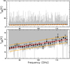Fig. A.1

Top panel: Continuum level derived with STATCONT overimposed to the GUAPOS spectrum. Bottom panel: y-axis zoom of the top panel. The red solid line represents the result from the linear regression fit, as explained in Appendix A, and the orange lines represent the erorr of ±1 K on the fit.

Appendix B Spectroscopy

The transitions of the molecules studied in this work (HNCO, HC(O)NH₂, CH₃NCO, CH₃C(O)NH₂, CH₃NHCHO, and CH₃CH₂NCO) were taken from the catalogues and spectroscopic works listed in Table B.1. We have taken the entries from the Cologne Database for Molecular Spectroscopy⁷(CDMS, Müller et al. 2001, 2005; Endres et al. 2016) and the Jet Propulsion Laboratory⁸ (JPL, Pickett et al. 1998) catalogues. Moreover, for species whose spectroscopy was not present in the catalogues, we have added to MADCUBA-SLIM entries using available spectroscopic works. A detailed explanation about how we evaluate the partition function of HNCO and CH₃CH₂NCO is given in Sects. B.1 and B.2, respectively.

B.1 HNCO data and partition function evaluation

The spectral predictions of HNCO in the three lowest vibrationally excited states (Brown et al. 1997), namely v₄ = 1 (E= 776.6 cm⁻¹), v₅ = 1 (E = 577.4 cm⁻¹), and v₆ = 1 (E = 656.3 cm⁻¹), have been obtained using the spectroscopic data reported in Yamada (1977); Yamada & Winnewisser (1977); Niedenhoff et al. (1996). The dipole moment components (μ_a = 1.58 D and μ_b = 1.35 D) were assumed to be identical to those determined for the ground vibrational state (Hocking et al. 1975).

The ro-vibrational partition function of HNCO has been computed at temperatures, T, between 2.725 and 300 K using the rotational partition function values from CDMS (see Col. 2 of Table B.2) and calculating the vibrational correction (Gordy et al. 1984) as: $Q_{vib} = {[\prod_{k = 1}^{3 N - 6} (1 - e^{- \frac{h ω_{k}}{k_{B} T}})]}^{- 1},$ $\begin{equation*}Q_{\mathrm{vib}} = \left[ \prod_{k=1}^{3N-6} \left(1 - e^{-\frac{h \omega_{\textrm{k}}}{k_{\textrm{B}} T}} \right) \right]^{-1} \,, \end{equation*}$ (B.1)

where ω_k is the vibrational harmonic frequency of the k-th vibrational mode, h is the Planck constant, and k_B is the Boltzmann constant. The sum runs over the k = 6 normal modes of HNCO, with the harmonic frequencies (ω_k) taken from Brown et al. (1997). The values of Q_vibrot are listed in Table B.2.

B.2 CH₃CH₂NCO data and partition function evaluation

The spectral predictions of C₂H₅NCO in the ground and the first three torsional excited states have been obtained using the recent spectroscopic data of Kolesniková et al. (2018), which also contain transitions from Heineking et al. (1994). The values of the dipole moment components, μ_a = 2.81(2) D and μ_b = 0.03 D, were derived in Sakaizumi et al. (1976).

In order to evaluate the ro-vibrational partition function of C₂H₅NCO, an approachsimilar to that used in Cernicharo et al. (2016) has been adopted. First, the rotational partition function was computed analytically using the following equation: $Q_{rot} (T) = 5.3311 \times 10^{6} \times \sqrt{\frac{T^{3}}{(A \times B \times C)}},$ $\begin{equation*}Q_{\mathrm{rot}}(T) = 5.3311 \times 10^6 \times\sqrt{\frac{T^3}{(A \times B \times C)}}, \end{equation*}$ (B.2)

where the factor 5.3311×10⁶ is derived from the units used for the temperature (T), K, and for the rotational constants A, B, and C, MHz. The values thus obtained were used to check whether the numerical computation of SPCAT (Pickett 1991) was close to convergence or not. The two methods gave comparable results, with differences smaller than 1%. Therefore, we decided to use the values computed numerically.

As far as the vibrational partition function is concerned, we decided to account for only the vibrational states below 400 cm⁻¹, as done by Cernicharo et al. (2016). This choice allowed a fair determination of the [CH₃NCO]/[C₂H₅NCO] abundance ratio.

CH₃CH₂NCO possesses three vibrational modes below 400 cm⁻¹ (~600 K), namely the C-N torsion (E = 40 cm⁻¹ Kolesniková et al. 2018), the CNC bending (E = 122 cm⁻¹ Durig et al. 2010), and the CH₃ torsion (E = 265 cm⁻¹ Durig et al. 2010). We considered all the multiple and combined excitations of these three modes within our threshold energy of 400 cm⁻¹ and computed the value of Q_vib at different temperatures using the following equation (Gordy et al. 1984): $Q_{vib} = \sum_{E_{i} = 0 {cm}^{- 1}}^{E_{i} \leq 400 {cm}^{- 1}} e^{- \frac{E_{i}}{k_{B} T}},$ $\begin{equation*}Q_{\mathrm{vib}} = \sum_{E_{\textrm{i}}=0~\mathrm{cm}^{-1}}^{E_i \le 400~\mathrm{cm}^{-1}} e^{-\frac{E_{\textrm{i}}}{k_{\textrm{B}} T}} \,, \end{equation*}$ (B.3)

where E_i is the vibrational energy of the i-th level. Finally, Q_vibrot was obtained as the product of Q_rot and Q_vib. All these values, computed at temperatures between 2.725 and 300 K, are listed in Table B.3.

Table B.1

Spectroscopy references for the molecules studied in this work.

Table B.2

Partition function values of HNCO computed at different temperatures.

Table B.3

Partition function values of C₂H₅NCO computed at different temperatures.

Appendix C Identified Spectral Lines

In this appendix we list the unblended or slightly blended transitions of the molecules studied in this work. These transitions are also shown in Figs. 2–9, D.1, D.2, D.3, and D.4. Table C1 is only available at the CDS.

Appendix D Tentative detections

In this appendix we show the transitions used for the fit of the v₄ =1 and v₅ =1 states of HNCO, of H¹⁵NCO, and of ¹³CH₃NCO.

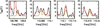Fig. D.1

Transitions listed in Table C.1 and used to fit the v₄=1 state of isocyanic acid (HNCO). The olive curve represents the best LTE fit obtained with MADCUBA (Table 1). The red curve shows the simulated spectrum taking into account all the species identified so far in the region.

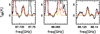Fig. D.2

Transitions listed in Table C.1 and used to fit the v₅=1 state of isocyanic acid (HNCO). The dark golden curve represents the best LTE fit obtained with MADCUBA (Table 1). The red curve shows the simulated spectrum taking into account all the species identified so far in the region.

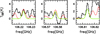Fig. D.3

Transitions listed in Table C.1 and used to fit H¹⁵NCO. The light green curve represents the best LTE fit obtained with MADCUBA (Table 1). The red curve shows the simulated spectrum taking into account all the species identified so far in the region.

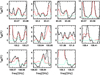Fig. D.4

Transitions listed in Table C.1 and used to fit ¹³CH₃NCO. The turquoise curve represents the best LTE fit obtained with MADCUBA (Table 1). The red curve shows the simulated spectrum taking into account all the species identified so far in the region. Note that at 108.406 GHz the baselinederived from STATCONT is slightly high, and the simulated spectra do not match exactly the observed one.

Appendix E Full GUAPOS spectrum

In this appendix we show the total observed spectra with the best LTE fit of the molecular species studied in this work. Moreover, the synthesised spectrum taking into account the contribution of all the possible molecular species is also shown.

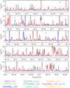Fig. E.1

Total spectrum of the GUAPOS project in black. The red curve shows the simulated spectrum taking into account all the species identified so far in the region. The best LTE fit of the molecules studied in this work is shown in different colours. The colour corresponding to each molecule is shown in the bottom panel. The coloured triangles indicate the transitions used to constrain the fitting procedure. Closer views of those transitions are given in Figs. 2–9.

References

Adams, F. C. 2010, ARA&A, 48, 47 [NASA ADS] [CrossRef] [Google Scholar]
Agarwal, V. K., Schutte, W., Greenberg, J. M., et al. 1985, Origins Life, 16, 21 [NASA ADS] [CrossRef] [Google Scholar]
Allen, V., van der Tak, F. F. S., López-Sepulcre, A., et al. 2020, A&A, 636, A67 [NASA ADS] [CrossRef] [EDP Sciences] [Google Scholar]
Altwegg, K., Balsiger, H., Berthelier, J. J., et al. 2017, MNRAS, 469, S130 [Google Scholar]
Arce, H. G., Santiago-García, J., Jørgensen, J. K., Tafalla, M., & Bachiller, R. 2008, ApJ, 681, L21 [NASA ADS] [CrossRef] [Google Scholar]
Bacmann, A., Taquet, V., Faure, A., Kahane, C., & Ceccarelli, C. 2012, A&A, 541, A12 [NASA ADS] [CrossRef] [EDP Sciences] [Google Scholar]
Barone, V., Latouche, C., Skouteris, D., et al. 2015, MNRAS, 453, L31 [Google Scholar]
Belloche, A., Müller, H. S. P., Menten, K. M., Schilke, P., & Comito, C. 2013, A&A, 559, A47 [NASA ADS] [CrossRef] [EDP Sciences] [Google Scholar]
Belloche, A., Müller, H. S. P., Garrod, R. T., & Menten, K. M. 2016, A&A, 587, A91 [NASA ADS] [CrossRef] [EDP Sciences] [Google Scholar]
Belloche, A., Meshcheryakov, A. A., Garrod, R. T., et al. 2017, A&A, 601, A49 [NASA ADS] [CrossRef] [EDP Sciences] [Google Scholar]
Belloche, A., Garrod, R. T., Müller, H. S. P., et al. 2019, A&A, 628, A10 [NASA ADS] [CrossRef] [EDP Sciences] [Google Scholar]
Belloche, A., Maury, A. J., Maret, S., et al. 2020, A&A, 635, A198 [CrossRef] [EDP Sciences] [Google Scholar]
Beltrán, M. T., Cesaroni, R., Neri, R., et al. 2005, A&A, 435, 901 [NASA ADS] [CrossRef] [EDP Sciences] [Google Scholar]
Beltrán, M. T., Codella, C., Viti, S., Neri, R., & Cesaroni, R. 2009, ApJ, 690, L93 [Google Scholar]
Beltrán, M. T., Olmi, L., Cesaroni, R., et al. 2013, A&A, 552, A123 [NASA ADS] [CrossRef] [EDP Sciences] [Google Scholar]
Beltrán, M. T., Cesaroni, R., Rivilla, V. M., et al. 2018, A&A, 615, A141 [NASA ADS] [CrossRef] [EDP Sciences] [Google Scholar]
Beltrán, M. T., Padovani, M., Girart, J. M., et al. 2019, A&A, 630, A54 [CrossRef] [EDP Sciences] [Google Scholar]
Beltrán, M. T., Rivilla, V. M., Cesaroni, R., et al. 2021, A&A, 648, A100 [Google Scholar]
Berger, R. 1961, Proc. Natl. Acad. Sci. U.S.A., 47, 1434 [NASA ADS] [CrossRef] [Google Scholar]
Bisschop, S. E., Jørgensen, J. K., van Dishoeck, E. F., & de Wachter, E. B. M. 2007, A&A, 465, 913 [NASA ADS] [CrossRef] [EDP Sciences] [Google Scholar]
Blanco, S., López, J. C., Lesarri, A., & Alonso, J. L. 2006, J. Am. Chem. Soc., 128, 12111 [CrossRef] [Google Scholar]
Bøgelund, E. G., McGuire, B. A., Ligterink, N. F. W., et al. 2018, A&A, 615, A88 [NASA ADS] [CrossRef] [EDP Sciences] [Google Scholar]
Bonal, L., Huss, G. R., Nagashima, K., & Krot, A. N. 2009, Meteoritics Planet. Sci. Suppl., 72, 5178 [Google Scholar]
Bonfand, M., Belloche, A., Garrod, R. T., et al. 2019, A&A, 628, A27 [NASA ADS] [CrossRef] [EDP Sciences] [Google Scholar]
Brown, R. D., Godfrey, P. D., & Storey, J. 1975, J. Mol. Spectrosc., 58, 445 [CrossRef] [Google Scholar]
Brown, S. S., Berghout, H. L., & Crim, F. F. 1997, J. Chem. Phys., 107, 9764 [CrossRef] [Google Scholar]
Canelo, C. M., Bronfman, L., Mendoza, E., et al. 2021, MNRAS, 504, 4428 [NASA ADS] [CrossRef] [Google Scholar]
Cassone, G., Saija, F., Sponer, J., et al. 2021, MNRAS, 504, 1565 [NASA ADS] [CrossRef] [Google Scholar]
Cernicharo, J., Kisiel, Z., Tercero, B., et al. 2016, A&A, 587, L4 [NASA ADS] [CrossRef] [EDP Sciences] [Google Scholar]
Cesaroni, R. 2019, A&A, 631, A65 [CrossRef] [EDP Sciences] [Google Scholar]
Cesaroni, R., Hofner, P., Araya, E., & Kurtz, S. 2010, A&A, 509, A50 [NASA ADS] [CrossRef] [EDP Sciences] [Google Scholar]
Cesaroni, R., Sánchez-Monge, Á., Beltrán, M. T., et al. 2017, A&A, 602, A59 [NASA ADS] [CrossRef] [EDP Sciences] [Google Scholar]
Charnley, S. B., Ehrenfreund, P., Millar, T. J., et al. 2004, MNRAS, 347, 157 [NASA ADS] [CrossRef] [Google Scholar]
Christiansen, J. J. 2005, J. Mol. Spectr., 231, 131 [NASA ADS] [CrossRef] [Google Scholar]
Codella, C., Ceccarelli, C., Bianchi, E., et al. 2020, A&A, 635, A17 [NASA ADS] [CrossRef] [EDP Sciences] [Google Scholar]
Coletta, A., Fontani, F., Rivilla, V. M., et al. 2020, A&A, 641, A54 [CrossRef] [EDP Sciences] [Google Scholar]
Colzi, L., Fontani, F., Rivilla, V. M., et al. 2018, MNRAS, 478, 3693 [NASA ADS] [CrossRef] [Google Scholar]
Cooper, G. W., & Cronin, J. R. 1995, Geochim. Cosmochim. Acta, 59, 1003 [CrossRef] [PubMed] [Google Scholar]
Corazzi, M. A., Fedele, D., Poggiali, G., & Brucato, J. R. 2020, A&A, 636, A63 [CrossRef] [EDP Sciences] [Google Scholar]
Coutens, A., Jørgensen, J. K., van der Wiel, M. H. D., et al. 2016, A&A, 590, A6 [NASA ADS] [CrossRef] [EDP Sciences] [Google Scholar]
Csengeri, T., Belloche, A., Bontemps, S., et al. 2019, A&A, 632, A57 [NASA ADS] [CrossRef] [EDP Sciences] [Google Scholar]
Cuadrado, S., Goicoechea, J. R., Cernicharo, J., et al. 2017, A&A, 603, A124 [NASA ADS] [CrossRef] [EDP Sciences] [Google Scholar]
Dulieu, F., Nguyen, T., Congiu, E., Baouche, S., & Taquet, V. 2019, MNRAS, 484, L119 [NASA ADS] [CrossRef] [Google Scholar]
Durig, J. R., Zhou, S. X., Zheng, C., & Durig, D. T. 2010, J. Mol. Struct., 971, 23 [NASA ADS] [CrossRef] [Google Scholar]
Endres, C. P., Schlemmer, S., Schilke, P., Stutzki, J., & Müller, H. S. P. 2016, J. Mol. Spectr., 327, 95 [NASA ADS] [CrossRef] [Google Scholar]
Fedoseev, G., Ioppolo, S., Zhao, D., Lamberts, T., & Linnartz, H. 2015, MNRAS, 446, 439 [NASA ADS] [CrossRef] [Google Scholar]
Fedoseev, G., Chuang, K. J., van Dishoeck, E. F., Ioppolo, S., & Linnartz, H. 2016, MNRAS, 460, 4297 [NASA ADS] [CrossRef] [Google Scholar]
Frigge, R., Zhu, C., Turner, A. M., et al. 2018, ApJ, 862, 84 [NASA ADS] [CrossRef] [Google Scholar]
Gardner, F. F., Godfrey, P. D., & Williams, D. R. 1980, MNRAS, 193, 713 [NASA ADS] [CrossRef] [Google Scholar]
Garrod, R. T., Widicus Weaver, S. L., & Herbst, E. 2008, ApJ, 682, 283 [NASA ADS] [CrossRef] [Google Scholar]
Girart, J. M., Beltrán, M. T., Zhang, Q., Rao, R., & Estalella, R. 2009, Science, 324, 1408 [NASA ADS] [CrossRef] [PubMed] [Google Scholar]
Gorai, P., Bhat, B., Sil, M., et al. 2020, ApJ, 895, 86 [Google Scholar]
Gorai, P., Das, A., Shimonishi, T., et al. 2021, ApJ, 907, 108 [NASA ADS] [CrossRef] [Google Scholar]
Gordy, W., Cook, R. L., & Weissberger, A. 1984, Microwave Molecular Spectra, (New York: Wiley) 18 [Google Scholar]
Grim, R. J. A., Greenberg, J. M., de Groot, M. S., et al. 1989, A&AS, 78, 161 [NASA ADS] [Google Scholar]
Guzmán, V. V., Goicoechea, J. R., Pety, J., et al. 2013, A&A, 560, A73 [NASA ADS] [CrossRef] [EDP Sciences] [Google Scholar]
Halfen, D. T., Ilyushin, V., & Ziurys, L. M. 2011, ApJ, 743, 60 [NASA ADS] [CrossRef] [Google Scholar]
Halfen, D. T., Ilyushin, V. V., & Ziurys, L. M. 2015, ApJ, 812, A5 [Google Scholar]
Haupa, K. A., Tarczay, G., & Lee, Y.-P. 2019, in 74th International Symposium on Molecular Spectroscopy [Google Scholar]
Heineking, N., Grabow, J.-U., & Stahl, W. 1994, Mol. Phys., 81, 1177 [NASA ADS] [CrossRef] [Google Scholar]
Helmich, F. P., & van Dishoeck, E. F. 1997, A&AS, 124, 205 [NASA ADS] [CrossRef] [EDP Sciences] [Google Scholar]
Hirota, E., Sugisaki, R., Nielsen, C. J., & Sørensen, G. O. 1974, J. Mol. Spectr., 49, 251 [NASA ADS] [CrossRef] [Google Scholar]
Hocking, W. H., Gerry, M. C. L., & Winnewisser, G. 1975, Can. J. Phys., 53, 1869 [NASA ADS] [CrossRef] [Google Scholar]
Hollis, J. M., Jewell, P. R., Lovas, F. J., Remijan, A., & Møllendal, H. 2004, ApJ, 610, L21 [Google Scholar]
Hollis, J. M., Lovas, F. J., Remijan, A. J., et al. 2006, ApJ, 643, L25 [Google Scholar]
Hunter, J. D. 2007, Comput. Sci. Eng., 9, 90 [NASA ADS] [CrossRef] [Google Scholar]
Ilyushin, V. V., Alekseev, E. A., Dyubko, S. F., Kleiner, I., & Hougen, J. T. 2004, J. Mol. Spectr., 227, 115 [NASA ADS] [CrossRef] [Google Scholar]
Immer, K., Li, J., Quiroga-Nuñez, L. H., et al. 2019, A&A, 632, A123 [CrossRef] [EDP Sciences] [Google Scholar]
Jiménez-Serra, I., Vasyunin, A. I., Caselli, P., et al. 2016, ApJ, 830, L6 [Google Scholar]
Jiménez-Serra, I., Martín-Pintado, J., Rivilla, V. M., et al. 2020, Astrobiology, 20, 1048 [Google Scholar]
Jones, B. M., Bennett, C. J., & Kaiser, R. I. 2011, ApJ, 734, 78 [NASA ADS] [CrossRef] [Google Scholar]
Jørgensen, J. K., Favre, C., Bisschop, S. E., et al. 2012, ApJ, 757, L4 [NASA ADS] [CrossRef] [Google Scholar]
Jørgensen, J. K., van der Wiel, M. H. D., Coutens, A., et al. 2016, A&A, 595, A117 [NASA ADS] [CrossRef] [EDP Sciences] [Google Scholar]
Jørgensen, J. K., Müller, H. S. P., Calcutt, H., et al. 2018, A&A, 620, A170 [NASA ADS] [CrossRef] [EDP Sciences] [Google Scholar]
Kasten, W., & Dreizler, H. 1986a, Z. Natur. Teil A, 41, 637 [NASA ADS] [CrossRef] [Google Scholar]
Kasten, W., & Dreizler, H. 1986b, Z. Natur. Teil A, 41, 1173 [NASA ADS] [CrossRef] [Google Scholar]
Kolesniková, L., Alonso, E. R., Tercero, B., Cernicharo, J., & Alonso, J. L. 2018, A&A, 616, A173 [Google Scholar]
Kolesniková, L., Kisiel, Z., Alonso, E. R., et al. 2019, ApJS, 245, 31 [Google Scholar]
Koput, J. 1986, J. Mol. Spectr., 115, 131 [NASA ADS] [CrossRef] [Google Scholar]
Korschinek, G., Faestermann, T., Poutivtsev, M., et al. 2020, Phys. Rev. Lett., 125, 031101 [NASA ADS] [CrossRef] [Google Scholar]
Kretschmer, U., Consalvo, D., Knaack, A., et al. 1996, Mol. Phys., 87, 1159 [NASA ADS] [CrossRef] [Google Scholar]
Kryvda, A. V., Gerasimov, V. G., Dyubko, S. F., Alekseev, E. A., & Motiyenko, R. A. 2009, J. Mol. Spectr., 254, 28 [NASA ADS] [CrossRef] [Google Scholar]
Kukolich, S. G., & Nelson, A. C. 1971, Chem. Phys. Lett., 11, 383 [NASA ADS] [CrossRef] [Google Scholar]
Kukolich, S. G., Nelson, A. C., & Yamanashi, B. S. 1971, J. Am. Chem. Soc., 93, 6769 [CrossRef] [Google Scholar]
Kurland, R. J., & Bright Wilson E., J. 1957, J. Chem. Phys., 27, 585 [NASA ADS] [CrossRef] [Google Scholar]
Lapinov, A. V., Golubiatnikov, G. Y., Markov, V. N., & Guarnieri, A. 2007, Astron. Lett., 33, 121 [NASA ADS] [CrossRef] [Google Scholar]
Lattelais, M., Pauzat, F., Ellinger, Y., & Ceccarelli, C. 2010, A&A, 519, A30 [NASA ADS] [CrossRef] [EDP Sciences] [Google Scholar]
Li, A., & Draine, B. T. 2001, ApJ, 554, 778 [Google Scholar]
Lichtenberg, T., Golabek, G. J., Burn, R., et al. 2019, Nat. Astron., 3, 307 [Google Scholar]
Ligterink, N. F. W., Coutens, A., Kofman, V., et al. 2017, MNRAS, 469, 2219 [NASA ADS] [CrossRef] [Google Scholar]
Ligterink, N. F. W., Terwisscha van Scheltinga, J., Taquet, V., et al. 2018, MNRAS, 480, 3628 [NASA ADS] [CrossRef] [Google Scholar]
Ligterink, N. F. W., El-Abd, S. J., Brogan, C. L., et al. 2020, ApJ, 901, 37 [Google Scholar]
Ligterink, N. F. W., Ahmadi, A., Coutens, A., et al. 2021, A&A, 647, A87 [NASA ADS] [CrossRef] [EDP Sciences] [Google Scholar]
López-Sepulcre, A., Jaber, A. A., Mendoza, E., et al. 2015, MNRAS, 449, 2438 [NASA ADS] [CrossRef] [Google Scholar]
López-Sepulcre, A., Balucani, N., Ceccarelli, C., et al. 2019, ACS Earth Space Chem., 3, 2122 [CrossRef] [Google Scholar]
Majumdar, L., Loison, J. C., Ruaud, M., et al. 2018, MNRAS, 473, L59 [CrossRef] [Google Scholar]
Manigand, S., Jørgensen, J. K., Calcutt, H., et al. 2020, A&A, 635, A48 [NASA ADS] [CrossRef] [EDP Sciences] [Google Scholar]
Marcelino, N., Cernicharo, J., Agúndez, M., et al. 2007, ApJ, 665, L127 [Google Scholar]
Maris, A. 2004, Physical Chemistry Chemical Physics (Incorporating Faraday Trans.), 6, 2611 [NASA ADS] [CrossRef] [Google Scholar]
Martín-Doménech, R., Rivilla, V. M., Jiménez-Serra, I., et al. 2017, MNRAS, 469, 2230 [NASA ADS] [CrossRef] [Google Scholar]
Martín-Doménech, R., Öberg, K. I., & Rajappan, M. 2020, ApJ, 894, 98 [Google Scholar]
Martín, S., Martín-Pintado, J., Blanco-Sánchez, C., et al. 2019, A&A, 631, A159 [NASA ADS] [CrossRef] [EDP Sciences] [Google Scholar]
McGuire, B. A. 2018, ApJS, 239, 17 [Google Scholar]
McMullin, J. P., Waters, B., Schiebel, D., Young, W., & Golap, K. 2007, in ASP Conf. Ser., 376, Astronomical Data Analysis Software and Systems XVI, eds. R. A. Shaw, F. Hill, & D. J. Bell, 127 [Google Scholar]
Mininni, C., Beltrán, M. T., Rivilla, V. M., et al. 2020, A&A, 644, A84 [EDP Sciences] [Google Scholar]
Miyake, K., & Nakagawa, Y. 1993, Icarus, 106, 20 [NASA ADS] [CrossRef] [Google Scholar]
Moskienko, E. M., & Dyubko, S. F. 1991, Radiophys. Quant. Electron., 34, 181 [NASA ADS] [CrossRef] [Google Scholar]
Motiyenko, R. A., Tercero, B., Cernicharo, J., & Margulès, L. 2012, A&A, 548, A71 [NASA ADS] [CrossRef] [EDP Sciences] [Google Scholar]
Müller, H. S. P., Thorwirth, S., Roth, D. A., & Winnewisser, G. 2001, A&A, 370, L49 [NASA ADS] [CrossRef] [EDP Sciences] [Google Scholar]
Müller, H. S. P., Schlöder, F., Stutzki, J., & Winnewisser, G. 2005, J. Mol. Struct., 742, 215 [Google Scholar]
Nazari, P., van Gelder, M. L., van Dishoeck, E. F., et al. 2021, A&A, 650, A150 [EDP Sciences] [Google Scholar]
Nguyen-Q-Rieu, Henkel, C., Jackson, J. M., & Mauersberger, R. 1991, A&A, 241, L33 [NASA ADS] [Google Scholar]
Nguyen, V. S., Abbott, H. L., Dawley, M. M., et al. 2011, J. Phys. Chem. A, 115, 841 [CrossRef] [Google Scholar]
Niedenhoff, M., Yamada, K. M. T., Belov, S. P., & Winnewisser, G. 1995, J. Mol. Spectr., 174, 151 [NASA ADS] [CrossRef] [Google Scholar]
Niedenhoff, M., Yamada, K., & Winnewisser, G. 1996, J. Mol. Spectrosc., 176, 342 [CrossRef] [Google Scholar]
Noble, J. A., Theule, P., Congiu, E., et al. 2015, A&A, 576, A91 [NASA ADS] [CrossRef] [EDP Sciences] [Google Scholar]
Osorio, M., Anglada, G., Lizano, S., & D’Alessio, P. 2009, ApJ, 694, 29 [Google Scholar]
Pascal, R., Boiteau, L., & Commeyras, A. 2005, From the Prebiotic Synthesis of α-Amino Acids Towards a PrimitiveTranslation Apparatus for the Synthesis of Peptides, ed. P. Walde (Berlin, Heidelberg: Springer Berlin Heidelberg), 69 [Google Scholar]
Pérez, L. M., Carpenter, J. M., Chand ler, C. J., et al. 2012, ApJ, 760, L17 [NASA ADS] [CrossRef] [Google Scholar]
Pickett, H. M. 1991, J. Mol. Spectrosc., 148, 371 [Google Scholar]
Pickett, H. M., Poynter, R. L., Cohen, E. A., et al. 1998, J. Quant. Spec. Radiat. Transf., 60, 883 [Google Scholar]
Quan, D., & Herbst, E. 2007, A&A, 474, 521 [NASA ADS] [CrossRef] [EDP Sciences] [Google Scholar]
Quénard, D., Jiménez-Serra, I., Viti, S., Holdship, J., & Coutens, A. 2018, MNRAS, 474, 2796 [NASA ADS] [CrossRef] [Google Scholar]
Raunier, S., Chiavassa, T., Duvernay, F., et al. 2004, A&A, 416, 165 [NASA ADS] [CrossRef] [EDP Sciences] [Google Scholar]
Redondo, P., Barrientos, C., & Largo, A. 2014, ApJ, 793, 32 [NASA ADS] [CrossRef] [Google Scholar]
Remijan, A. J., Snyder, L. E., McGuire, B. A., et al. 2014, ApJ, 783, 77 [Google Scholar]
Requena-Torres, M. A., Martín-Pintado, J., Rodríguez-Franco, A., et al. 2006, A&A, 455, 971 [NASA ADS] [CrossRef] [EDP Sciences] [Google Scholar]
Rimola, A., Skouteris, D., Balucani, N., et al. 2018, ACS Earth Space Chem., 2, 720 [Google Scholar]
Rivilla, V. M., Beltrán, M. T., Cesaroni, R., et al. 2017, A&A, 598, A59 [NASA ADS] [CrossRef] [EDP Sciences] [Google Scholar]
Rivilla, V. M., Martín-Pintado, J., Jiménez-Serra, I., et al. 2019, MNRAS, 483, L114 [NASA ADS] [CrossRef] [Google Scholar]
Rivilla, V. M., Jiménez-Serra, I., Martín-Pintado, J., et al. 2021, Proc. Natl. Acad. Sci. U.S.A., 118, https://www.pnas.org/content/118/22/e2101314118.full.pdf [Google Scholar]
Rodríguez-Almeida, L. F., Jiménez-Serra, I., Rivilla, V. M., et al. 2021, ApJ, 912, L11 [Google Scholar]
Rodríguez-Fernández, N. J., Tafalla, M., Gueth, F., & Bachiller, R. 2010, A&A, 516, A98 [NASA ADS] [CrossRef] [EDP Sciences] [Google Scholar]
Rolffs, R., Schilke, P., Zhang, Q., & Zapata, L. 2011, A&A, 536, A33 [NASA ADS] [CrossRef] [EDP Sciences] [Google Scholar]
Sakaizumi, T., Yamada, O., Ushida, K., Ohashi, O., & Yamaguchi, I. 1976, Bull. Chem. Soc. Jpn., 49, 2908 [Google Scholar]
Sánchez-Monge, Á., Schilke, P., Ginsburg, A., Cesaroni, R., & Schmiedeke, A. 2018, A&A, 609, A101 [NASA ADS] [CrossRef] [EDP Sciences] [Google Scholar]
Sanz-Novo, M., Belloche, A., Alonso, J. L., et al. 2020, A&A, 639, A135 [CrossRef] [EDP Sciences] [Google Scholar]
Skouteris, D., Vazart, F., Ceccarelli, C., et al. 2017, MNRAS, 468, L1 [NASA ADS] [Google Scholar]
Snyder, L. E.,& Buhl, D. 1972, ApJ, 177, 619 [NASA ADS] [CrossRef] [Google Scholar]
Stubgaard, M. 1978, PhD Thesis, Københavns Universitet, Denmark [Google Scholar]
Suhasaria, T., & Mennella, V. 2020, A&A, 641, A88 [NASA ADS] [CrossRef] [EDP Sciences] [Google Scholar]
Tielens, A. G. G. M., & Hagen, W. 1982, A&A, 114, 245 [Google Scholar]
Turner, B. E., Terzieva, R., & Herbst, E. 1999, ApJ, 518, 699 [NASA ADS] [CrossRef] [Google Scholar]
Vorob’eva, E. M., & Dyubko, S. F. 1994, Radiophys. Quant. Electron., 37, 155 [Google Scholar]
Wallner, A., Feige, J., Fifield, L. K., et al. 2020, Proc. Natl. Acad. Sci. U.S.A., 117, 21873 [CrossRef] [Google Scholar]
Wilson, T. L. 1999, Rep. Prog. Phys., 62, 143 [Google Scholar]
Wilson, T. L.,& Rood, R. 1994, ARA&A, 32, 191 [Google Scholar]
Winnewisser, M., Medvedev, I. R., De Lucia, F. C., et al. 2005, ApJS, 159, 189 [NASA ADS] [CrossRef] [Google Scholar]
Yamada, K. 1977, J. Mol. Spectrosc., 68, 423 [NASA ADS] [CrossRef] [Google Scholar]
Yamada, K., & Winnewisser, M. 1977, J. Mol. Spectrosc., 68, 307 [NASA ADS] [CrossRef] [Google Scholar]
Yan, Y. T., Zhang, J. S., Henkel, C., et al. 2019, ApJ, 877, 154 [Google Scholar]
Zeng, S., Jiménez-Serra, I., Rivilla, V. M., et al. 2018, MNRAS, 478, 2962 [NASA ADS] [CrossRef] [Google Scholar]
Zeng, S., Zhang, Q., Jiménez-Serra, I., et al. 2020, MNRAS, 497, 4896 [NASA ADS] [CrossRef] [Google Scholar]

¹

STATCONT is freely accessible here: https://hera.ph1.uni-koeln.de/~sanchez/statcont

²

Madrid Data Cube Analysis on ImageJ is a software developed at the Center for Astrobiology (CAB) in Madrid; https://cab.inta-csic.es/madcuba/index.html

³

http://cdms.astro.uni-koeln.de/classic/

⁴

https://spec.jpl.nasa.gov/ftp/pub/catalog/catdir.html

⁵

https://casa.nrao.edu

⁶

It is a doublet transition that is not resolved in frequency because the line width (~8 km s⁻¹) is higher than the spectral separation between the two lines (1.8 × 10⁻³ km s⁻¹ at 219.656 GHz).

⁷

http://cdms.astro.uni-koeln.de/classic/.

⁸

https://spec.jpl.nasa.gov/ftp/pub/catalog/catdir.html.

All Tables

Table 1

Line parameters obtained from the best LTE fit and abundance for HNCO, HC(O)NH₂, CH₃NCO (and their ¹³C-isotopologues), CH₃C(O)NH₂, CH₃NHCHO, CH₃CH₂NCO, NH₂C(O)NH₂, NH₂C(O)CN, and HOCH₂C(O)NH₂.

In the text

Table B.1

Spectroscopy references for the molecules studied in this work.

In the text

Table B.2

Partition function values of HNCO computed at different temperatures.

In the text

Table B.3

Partition function values of C₂H₅NCO computed at different temperatures.

In the text

All Figures

	Fig. 1 Chemical structure of the peptide-like bond molecules studied in this paper. White, grey, red, and blue spheres correspond to H, C, O, and N atoms, respectively.
In the text

	Fig. 2 Transitions listed in Table C.1 and used to fit the v = 0 state of isocyanic acid (HNCO) and its ¹³C-isotopologue (HN¹³ CO). The magenta and green curves represent the best LTE fits obtained with MADCUBA for HNCO and HN¹³ CO, respectively (Table 1). The red curve shows the simulated spectrum taking into account all the species identified so far in the region.
In the text

	Fig. 3 Transitions listed in Table C.1 and used to fit the v = 0 state of formamide (HC(O)NH₂). The blue curve represents the best LTE fit obtained with MADCUBA (Table 1). The red curve shows the simulated spectrum taking into account all the species identified so far in the region.
In the text

	Fig. 4 Transitions listed in Table C.1 and used to fit the v = 0 state of the ¹³C-isotopologue of formamide (H¹³C(O)NH₂). The dark green curve represents the best LTE fit obtained with MADCUBA (Table 1). The red curve shows the simulated spectrum taking into account all the species identified so far in the region.
In the text

	Fig. 5 Transitions listed in Table C.1 and used to fit the v₁₂ = 1 state of formamide (HC(O)NH₂). The steel blue curve represents the best LTE fits obtained with MADCUBA (Table 1). The red curve shows the simulated spectrum taking into account all the species identified so far in the region.
In the text

	Fig. 6 Transitions listed in Table C.1 and used to fit the v_b = 0 state of methyl isocyanate (CH₃NCO). The dark turquoise curve represents the best LTE fit obtained with MADCUBA (Table 1). The red curve shows the simulated spectrum taking into account all the species identified so far in the region.
In the text

	Fig. 7 Transitions listed in Table C.1 and used to fit the v_b = 1 state of methyl isocyanate (CH₃NCO). The light orange curve represents the best LTE fits obtained with MADCUBA (Table 1). The red curve shows the simulated spectrum taking into account all the species identified so far in the region.
In the text

	Fig. 8 Transitions listed in Table C.1 and used to fit the v = 0, and v_t = 1, 2 states of acetamide (CH₃C(O)NH₂). The purple curve represents the best LTE fit obtained with MADCUBA (Table 1). The red curve shows the simulated spectrum taking into account all the species identified so far in the region.
In the text

	Fig. 9 Transitions listed in Table C.1 and used to fit the v = 0 state of N-methylformamide (CH₃NHCHO). The gold curve represents the best LTE fit obtained with MADCUBA (Table 1). The red curve shows the simulated spectrum taking into account all the species identified so far in the region.
In the text

Fig. 10

ALMA 1.′′2 resolution integrated emission maps at 3 mm of transitions with different E_up (from 0 up to 200 K, different columns) of HC(O)NH₂, HNCO, CH₃NCO, CH₃C(O)NH₂, and CH₃NHCHO (different rows) obtained with the GUAPOS survey. In each panel, the white contours show the continuum emission levels at 5, 10, 20, 40, 60, 100, and 200 times the rms value of 0.8 mJy beam⁻¹. The white ellipse in the lower left corner represents the synthesised beam.

In the text

	Fig. 11 Maps of the integrated emission for the molecules studied in this paper. Different colours within the same panel represent the range of upper energy levels of the transitions taken into account. The contours represents 0.5 times the integrated emission peak level of the corresponding map. The beam is indicated in the left-bottom corner of the maps.
In the text

	Fig. 12 Maps of the integrated emission for the molecules studied in this paper. Different colours within the same panel represent different molecules. The contours represents 0.5 times the integrated emission peak level of the corresponding map. The beam is indicated in the left-bottom corner of the maps.
In the text

Fig. 13

ALMA 0.′′2 resolution integrated emission maps at 1.4 mm of HC(O)NH₂ (10_1,9–9_1,8) (top-left panel), CH₃NCO (25_2,23,0–24_2,22,0 and 25_−3,−,1–24_−3,−,1) (top-right panel), HNCO (10_3,8–9_3,7 and 10_3,7–9_3,6) (bottom-left panel), and HNCO (10_1,9–9_1,8) (bottom-right panel) in a velocity range between 93 and 100 km s⁻¹ for each transition. The contour levels are 0.3, 0.4, 0.5, 0.6, 0.7, 0.8, and 0.9 the maximum value of the maps. The maximum values of the maps are 1.625 Jy beam⁻¹ km s⁻¹ for HC(O)NH₂, 0.877 Jy beam⁻¹ km s⁻¹for CH₃NCO, 1.082 Jy beam⁻¹ km s⁻¹ for HNCO at219.656 GHz, and 1.396 Jy beam⁻¹ km s⁻¹ for HNCO at 220.585 GHz. The black dashed circle indicates in all the panels the area in which the spectrum analysed in this work was extracted, which matches the GUAPOS beam of 1.′′ 2 centered at the 3mm continuum peak. The frequency and E_up energies of the transitions are shown in blue above each panel, and in red in the top-right corner of each panel, respectively.The synthesised beam is represented by the grey ellipse in the lower left corner. The black squares indicates the position of the continuum sources A, B, C, and D resolved with 7 mm VLA observations by Beltrán et al. (2021).

In the text

Fig. 14

Molecular abundances (X) with respect to H₂ towards G31, G10.47, G328.2551 A, B, and env, Sgr B2(N2), Sgr B2(N5), IRAS 16293 B (upper limits), and G+0.693. Different colours represent the different molecules for which the abundances are shown, as indicated in the legend in the upper-right corner. Data are taken from: G31 (this work), G10.47 (Gorai et al. 2020), G328.2551 (Csengeri et al. 2019), Sgr B2(N2) (Belloche et al. 2017), Sgr B2(N5) (Bonfand et al. 2019), IRAS 16293 B (Martín-Doménech et al. 2017), and G+0.693 (Zeng et al. 2018) (from the left to the right).

In the text

Fig. 15

Upper-left panel: X[HC(O)NH₂] as a functionof X[HNCO]. The solid line is the power-law fit obtained in this work, while the dashed and pointed lines are those obtained by López-Sepulcre et al. (2015) and Quénard et al. (2018), respectively. Upper-right panel: X[CH₃NCO] as a functionof X[HNCO]. The solid line is the power-law fit obtained in this work. Lower panel: X[CH₃NCO] as a functionof X[HC(O)NH₂]. The solid line is the power-law fit obtained in this work. In all the panels, the different colours represent the different sources, as indicated in the bottom-right legend. Data are taken from the same works indicated in Fig. 14.

In the text

Fig. 16

Molecular abundances with respect to CH₃OH towards G31, G328.2551 A, B, and env, Sgr B2(N), Sgr B2(N2), Sgr B2(N3), Sgr B2(N5), NGC 6334I MM1-i–v and MM2-i–ii, Orion BN/KL A and B, IRAS 16293 A and B, and G+0.693. Different colours represent the different molecules for which the abundances are shown, as indicated in the legend in the upper-left corner. Data are taken from: G31 (this work, Mininni et al. in prep.), G328.2551 (Csengeri et al. 2019), Sgr B2(N) (Belloche et al. 2013), Sgr B2(N2) (Belloche et al. 2016, 2017), Sgr B2(N3) and Sgr B2(N5) (Bonfand et al. 2019), NGC 6334I (Bøgelund et al. 2018; Ligterink et al. 2020), Orion BN/KL A and B (Cernicharo et al. 2016), IRAS 16293 A (Ligterink et al. 2017; Manigand et al. 2020), IRAS 16293 B (Ligterink et al. 2017, 2018; Jørgensen et al. 2018), and G+0.693 (Zeng et al. 2018; Rodríguez-Almeida et al. 2021) (from the left to the right).

In the text

Fig. 17

Upper-left panel: $X_{{CH}_{3} OH}$ $X_{\textrm{CH}_{3}\textrm{OH}}$ (HC(O)NH₂) as a functionof $X_{{CH}_{3} OH}$ $X_{\textrm{CH}_{3}\textrm{OH}}$ (HNCO). Upper-central panel: $X_{{CH}_{3} OH}$ $X_{\textrm{CH}_{3}\textrm{OH}}$ (CH₃NCO) as a functionof $X_{{CH}_{3} OH}$ $X_{\textrm{CH}_{3}\textrm{OH}}$ (HNCO). Upper-right panel: $X_{{CH}_{3} OH}$ $X_{\textrm{CH}_{3}\textrm{OH}}$ (CH₃NCO) as a functionof $X_{{CH}_{3} OH}$ $X_{\textrm{CH}_{3}\textrm{OH}}$ (HC(O)NH₂). Bottom-left panel: $X_{{CH}_{3} OH}$ $X_{\textrm{CH}_{3}\textrm{OH}}$ (CH₃C(O)NH₂) as a functionof $X_{{CH}_{3} OH}$ $X_{\textrm{CH}_{3}\textrm{OH}}$ (HNCO). Bottom-central panel: $X_{{CH}_{3} OH}$ $X_{\textrm{CH}_{3}\textrm{OH}}$ (CH₃C(O)NH₂) as a functionof $X_{{CH}_{3} OH}$ $X_{\textrm{CH}_{3}\textrm{OH}}$ (HC(O)NH₂). In all the panels, the solid lines are the power-law fit obtained in this work, and the different colours represent the different sources, as indicated in the bottom-right legend. Data are taken from the same works indicated in Fig. 16.

In the text

Fig. 18

HNCO, CH₃NCO, CH₃C(O)NH₂, and CH₃NHCHO column density ratios with respect to HC(O)NH₂ (upper-left, upper-right, bottom-left, and bottom-right panels, respectively) towards G31 (red points and shaded areas) and high- and low-mass star-forming regions, a GC molecular cloud, and the 67P comet (from the left to the right in all panels). Different colours represent: G31 in red, Sgr B2 in blue, Orion BN/KL in green, NGC 6334I in purple, G10.47 in grey, G328.2551 in brown, IRAS 16293 in light blue, G+0.693 in orange, and the comet 67P in black. Data are taken from: G31 (this work), Sgr B2(N) (Belloche et al. 2013), Sgr B2(N2) (Belloche et al. 2017), Sgr B2(N1S) (Belloche et al. 2019), Sgr B2(N3) and Sgr B2(N5) (Bonfand et al. 2019), Orion BN/KL - A and B (Cernicharo et al. 2016), NGC 6334I MM1-i–MM2ii (Ligterink et al. 2020), G10.47 (Gorai et al. 2020), G328.2551 A, B and env (Csengeri et al. 2019), IRAS 16293 A and B (Ligterink et al. 2017; Manigand et al. 2020; Ligterink et al. 2018; Martín-Doménech et al. 2017); G+0.693 (Zeng et al. 2018), and comet 67P (Altwegg et al. 2017) (from the left to the right).

In the text

	Fig. A.1 Top panel: Continuum level derived with STATCONT overimposed to the GUAPOS spectrum. Bottom panel: y-axis zoom of the top panel. The red solid line represents the result from the linear regression fit, as explained in Appendix A, and the orange lines represent the erorr of ±1 K on the fit.
In the text

	Fig. D.1 Transitions listed in Table C.1 and used to fit the v₄=1 state of isocyanic acid (HNCO). The olive curve represents the best LTE fit obtained with MADCUBA (Table 1). The red curve shows the simulated spectrum taking into account all the species identified so far in the region.
In the text

	Fig. D.2 Transitions listed in Table C.1 and used to fit the v₅=1 state of isocyanic acid (HNCO). The dark golden curve represents the best LTE fit obtained with MADCUBA (Table 1). The red curve shows the simulated spectrum taking into account all the species identified so far in the region.
In the text

	Fig. D.3 Transitions listed in Table C.1 and used to fit H¹⁵NCO. The light green curve represents the best LTE fit obtained with MADCUBA (Table 1). The red curve shows the simulated spectrum taking into account all the species identified so far in the region.
In the text

Fig. D.4

Transitions listed in Table C.1 and used to fit ¹³CH₃NCO. The turquoise curve represents the best LTE fit obtained with MADCUBA (Table 1). The red curve shows the simulated spectrum taking into account all the species identified so far in the region. Note that at 108.406 GHz the baselinederived from STATCONT is slightly high, and the simulated spectra do not match exactly the observed one.

In the text

Fig. E.1

Total spectrum of the GUAPOS project in black. The red curve shows the simulated spectrum taking into account all the species identified so far in the region. The best LTE fit of the molecules studied in this work is shown in different colours. The colour corresponding to each molecule is shown in the bottom panel. The coloured triangles indicate the transitions used to constrain the fitting procedure. Closer views of those transitions are given in Figs. 2–9.

In the text

Current usage metrics show cumulative count of Article Views (full-text article views including HTML views, PDF and ePub downloads, according to the available data) and Abstracts Views on Vision4Press platform.

Data correspond to usage on the plateform after 2015. The current usage metrics is available 48-96 hours after online publication and is updated daily on week days.

Initial download of the metrics may take a while.

[1] Adams, F. C. 2010, ARA&A, 48, 47 [NASA ADS] [CrossRef] [Google Scholar]

[2] Agarwal, V. K., Schutte, W., Greenberg, J. M., et al. 1985, Origins Life, 16, 21 [NASA ADS] [CrossRef] [Google Scholar]

[3] Allen, V., van der Tak, F. F. S., López-Sepulcre, A., et al. 2020, A&A, 636, A67 [NASA ADS] [CrossRef] [EDP Sciences] [Google Scholar]

[4] Altwegg, K., Balsiger, H., Berthelier, J. J., et al. 2017, MNRAS, 469, S130 [Google Scholar]

[5] Arce, H. G., Santiago-García, J., Jørgensen, J. K., Tafalla, M., & Bachiller, R. 2008, ApJ, 681, L21 [NASA ADS] [CrossRef] [Google Scholar]

[6] Bacmann, A., Taquet, V., Faure, A., Kahane, C., & Ceccarelli, C. 2012, A&A, 541, A12 [NASA ADS] [CrossRef] [EDP Sciences] [Google Scholar]

[7] Barone, V., Latouche, C., Skouteris, D., et al. 2015, MNRAS, 453, L31 [Google Scholar]

[8] Belloche, A., Müller, H. S. P., Menten, K. M., Schilke, P., & Comito, C. 2013, A&A, 559, A47 [NASA ADS] [CrossRef] [EDP Sciences] [Google Scholar]

[9] Belloche, A., Müller, H. S. P., Garrod, R. T., & Menten, K. M. 2016, A&A, 587, A91 [NASA ADS] [CrossRef] [EDP Sciences] [Google Scholar]

[10] Belloche, A., Meshcheryakov, A. A., Garrod, R. T., et al. 2017, A&A, 601, A49 [NASA ADS] [CrossRef] [EDP Sciences] [Google Scholar]

[11] Belloche, A., Garrod, R. T., Müller, H. S. P., et al. 2019, A&A, 628, A10 [NASA ADS] [CrossRef] [EDP Sciences] [Google Scholar]

[12] Belloche, A., Maury, A. J., Maret, S., et al. 2020, A&A, 635, A198 [CrossRef] [EDP Sciences] [Google Scholar]

[13] Beltrán, M. T., Cesaroni, R., Neri, R., et al. 2005, A&A, 435, 901 [NASA ADS] [CrossRef] [EDP Sciences] [Google Scholar]

[14] Beltrán, M. T., Codella, C., Viti, S., Neri, R., & Cesaroni, R. 2009, ApJ, 690, L93 [Google Scholar]

[15] Beltrán, M. T., Olmi, L., Cesaroni, R., et al. 2013, A&A, 552, A123 [NASA ADS] [CrossRef] [EDP Sciences] [Google Scholar]

[16] Beltrán, M. T., Cesaroni, R., Rivilla, V. M., et al. 2018, A&A, 615, A141 [NASA ADS] [CrossRef] [EDP Sciences] [Google Scholar]

[17] Beltrán, M. T., Padovani, M., Girart, J. M., et al. 2019, A&A, 630, A54 [CrossRef] [EDP Sciences] [Google Scholar]

[18] Beltrán, M. T., Rivilla, V. M., Cesaroni, R., et al. 2021, A&A, 648, A100 [Google Scholar]

[19] Berger, R. 1961, Proc. Natl. Acad. Sci. U.S.A., 47, 1434 [NASA ADS] [CrossRef] [Google Scholar]

[20] Bisschop, S. E., Jørgensen, J. K., van Dishoeck, E. F., & de Wachter, E. B. M. 2007, A&A, 465, 913 [NASA ADS] [CrossRef] [EDP Sciences] [Google Scholar]

[21] Blanco, S., López, J. C., Lesarri, A., & Alonso, J. L. 2006, J. Am. Chem. Soc., 128, 12111 [CrossRef] [Google Scholar]

[22] Bøgelund, E. G., McGuire, B. A., Ligterink, N. F. W., et al. 2018, A&A, 615, A88 [NASA ADS] [CrossRef] [EDP Sciences] [Google Scholar]

[23] Bonal, L., Huss, G. R., Nagashima, K., & Krot, A. N. 2009, Meteoritics Planet. Sci. Suppl., 72, 5178 [Google Scholar]

[24] Bonfand, M., Belloche, A., Garrod, R. T., et al. 2019, A&A, 628, A27 [NASA ADS] [CrossRef] [EDP Sciences] [Google Scholar]

[25] Brown, R. D., Godfrey, P. D., & Storey, J. 1975, J. Mol. Spectrosc., 58, 445 [CrossRef] [Google Scholar]

[26] Brown, S. S., Berghout, H. L., & Crim, F. F. 1997, J. Chem. Phys., 107, 9764 [CrossRef] [Google Scholar]

[27] Canelo, C. M., Bronfman, L., Mendoza, E., et al. 2021, MNRAS, 504, 4428 [NASA ADS] [CrossRef] [Google Scholar]

[28] Cassone, G., Saija, F., Sponer, J., et al. 2021, MNRAS, 504, 1565 [NASA ADS] [CrossRef] [Google Scholar]

[29] Cernicharo, J., Kisiel, Z., Tercero, B., et al. 2016, A&A, 587, L4 [NASA ADS] [CrossRef] [EDP Sciences] [Google Scholar]

[30] Cesaroni, R. 2019, A&A, 631, A65 [CrossRef] [EDP Sciences] [Google Scholar]

[31] Cesaroni, R., Hofner, P., Araya, E., & Kurtz, S. 2010, A&A, 509, A50 [NASA ADS] [CrossRef] [EDP Sciences] [Google Scholar]

[32] Cesaroni, R., Sánchez-Monge, Á., Beltrán, M. T., et al. 2017, A&A, 602, A59 [NASA ADS] [CrossRef] [EDP Sciences] [Google Scholar]

[33] Charnley, S. B., Ehrenfreund, P., Millar, T. J., et al. 2004, MNRAS, 347, 157 [NASA ADS] [CrossRef] [Google Scholar]

[34] Christiansen, J. J. 2005, J. Mol. Spectr., 231, 131 [NASA ADS] [CrossRef] [Google Scholar]

[35] Codella, C., Ceccarelli, C., Bianchi, E., et al. 2020, A&A, 635, A17 [NASA ADS] [CrossRef] [EDP Sciences] [Google Scholar]

[36] Coletta, A., Fontani, F., Rivilla, V. M., et al. 2020, A&A, 641, A54 [CrossRef] [EDP Sciences] [Google Scholar]

[37] Colzi, L., Fontani, F., Rivilla, V. M., et al. 2018, MNRAS, 478, 3693 [NASA ADS] [CrossRef] [Google Scholar]

[38] Cooper, G. W., & Cronin, J. R. 1995, Geochim. Cosmochim. Acta, 59, 1003 [CrossRef] [PubMed] [Google Scholar]

[39] Corazzi, M. A., Fedele, D., Poggiali, G., & Brucato, J. R. 2020, A&A, 636, A63 [CrossRef] [EDP Sciences] [Google Scholar]

[40] Coutens, A., Jørgensen, J. K., van der Wiel, M. H. D., et al. 2016, A&A, 590, A6 [NASA ADS] [CrossRef] [EDP Sciences] [Google Scholar]

[41] Csengeri, T., Belloche, A., Bontemps, S., et al. 2019, A&A, 632, A57 [NASA ADS] [CrossRef] [EDP Sciences] [Google Scholar]

[42] Cuadrado, S., Goicoechea, J. R., Cernicharo, J., et al. 2017, A&A, 603, A124 [NASA ADS] [CrossRef] [EDP Sciences] [Google Scholar]

[43] Dulieu, F., Nguyen, T., Congiu, E., Baouche, S., & Taquet, V. 2019, MNRAS, 484, L119 [NASA ADS] [CrossRef] [Google Scholar]

[44] Durig, J. R., Zhou, S. X., Zheng, C., & Durig, D. T. 2010, J. Mol. Struct., 971, 23 [NASA ADS] [CrossRef] [Google Scholar]

[45] Endres, C. P., Schlemmer, S., Schilke, P., Stutzki, J., & Müller, H. S. P. 2016, J. Mol. Spectr., 327, 95 [NASA ADS] [CrossRef] [Google Scholar]

[46] Fedoseev, G., Ioppolo, S., Zhao, D., Lamberts, T., & Linnartz, H. 2015, MNRAS, 446, 439 [NASA ADS] [CrossRef] [Google Scholar]

[47] Fedoseev, G., Chuang, K. J., van Dishoeck, E. F., Ioppolo, S., & Linnartz, H. 2016, MNRAS, 460, 4297 [NASA ADS] [CrossRef] [Google Scholar]

[48] Frigge, R., Zhu, C., Turner, A. M., et al. 2018, ApJ, 862, 84 [NASA ADS] [CrossRef] [Google Scholar]

[49] Gardner, F. F., Godfrey, P. D., & Williams, D. R. 1980, MNRAS, 193, 713 [NASA ADS] [CrossRef] [Google Scholar]

[50] Garrod, R. T., Widicus Weaver, S. L., & Herbst, E. 2008, ApJ, 682, 283 [NASA ADS] [CrossRef] [Google Scholar]

[51] Girart, J. M., Beltrán, M. T., Zhang, Q., Rao, R., & Estalella, R. 2009, Science, 324, 1408 [NASA ADS] [CrossRef] [PubMed] [Google Scholar]

[52] Gorai, P., Bhat, B., Sil, M., et al. 2020, ApJ, 895, 86 [Google Scholar]

[53] Gorai, P., Das, A., Shimonishi, T., et al. 2021, ApJ, 907, 108 [NASA ADS] [CrossRef] [Google Scholar]

[54] Gordy, W., Cook, R. L., & Weissberger, A. 1984, Microwave Molecular Spectra, (New York: Wiley) 18 [Google Scholar]

[55] Grim, R. J. A., Greenberg, J. M., de Groot, M. S., et al. 1989, A&AS, 78, 161 [NASA ADS] [Google Scholar]

[56] Guzmán, V. V., Goicoechea, J. R., Pety, J., et al. 2013, A&A, 560, A73 [NASA ADS] [CrossRef] [EDP Sciences] [Google Scholar]

[57] Halfen, D. T., Ilyushin, V., & Ziurys, L. M. 2011, ApJ, 743, 60 [NASA ADS] [CrossRef] [Google Scholar]

[58] Halfen, D. T., Ilyushin, V. V., & Ziurys, L. M. 2015, ApJ, 812, A5 [Google Scholar]

[59] Haupa, K. A., Tarczay, G., & Lee, Y.-P. 2019, in 74th International Symposium on Molecular Spectroscopy [Google Scholar]

[60] Heineking, N., Grabow, J.-U., & Stahl, W. 1994, Mol. Phys., 81, 1177 [NASA ADS] [CrossRef] [Google Scholar]

[61] Helmich, F. P., & van Dishoeck, E. F. 1997, A&AS, 124, 205 [NASA ADS] [CrossRef] [EDP Sciences] [Google Scholar]

[62] Hirota, E., Sugisaki, R., Nielsen, C. J., & Sørensen, G. O. 1974, J. Mol. Spectr., 49, 251 [NASA ADS] [CrossRef] [Google Scholar]

[63] Hocking, W. H., Gerry, M. C. L., & Winnewisser, G. 1975, Can. J. Phys., 53, 1869 [NASA ADS] [CrossRef] [Google Scholar]

[64] Hollis, J. M., Jewell, P. R., Lovas, F. J., Remijan, A., & Møllendal, H. 2004, ApJ, 610, L21 [Google Scholar]

[65] Hollis, J. M., Lovas, F. J., Remijan, A. J., et al. 2006, ApJ, 643, L25 [Google Scholar]

[66] Hunter, J. D. 2007, Comput. Sci. Eng., 9, 90 [NASA ADS] [CrossRef] [Google Scholar]

[67] Ilyushin, V. V., Alekseev, E. A., Dyubko, S. F., Kleiner, I., & Hougen, J. T. 2004, J. Mol. Spectr., 227, 115 [NASA ADS] [CrossRef] [Google Scholar]

[68] Immer, K., Li, J., Quiroga-Nuñez, L. H., et al. 2019, A&A, 632, A123 [CrossRef] [EDP Sciences] [Google Scholar]

[69] Jiménez-Serra, I., Vasyunin, A. I., Caselli, P., et al. 2016, ApJ, 830, L6 [Google Scholar]

[70] Jiménez-Serra, I., Martín-Pintado, J., Rivilla, V. M., et al. 2020, Astrobiology, 20, 1048 [Google Scholar]

[71] Jones, B. M., Bennett, C. J., & Kaiser, R. I. 2011, ApJ, 734, 78 [NASA ADS] [CrossRef] [Google Scholar]

[72] Jørgensen, J. K., Favre, C., Bisschop, S. E., et al. 2012, ApJ, 757, L4 [NASA ADS] [CrossRef] [Google Scholar]

[73] Jørgensen, J. K., van der Wiel, M. H. D., Coutens, A., et al. 2016, A&A, 595, A117 [NASA ADS] [CrossRef] [EDP Sciences] [Google Scholar]

[74] Jørgensen, J. K., Müller, H. S. P., Calcutt, H., et al. 2018, A&A, 620, A170 [NASA ADS] [CrossRef] [EDP Sciences] [Google Scholar]

[75] Kasten, W., & Dreizler, H. 1986a, Z. Natur. Teil A, 41, 637 [NASA ADS] [CrossRef] [Google Scholar]

[76] Kasten, W., & Dreizler, H. 1986b, Z. Natur. Teil A, 41, 1173 [NASA ADS] [CrossRef] [Google Scholar]

[77] Kolesniková, L., Alonso, E. R., Tercero, B., Cernicharo, J., & Alonso, J. L. 2018, A&A, 616, A173 [Google Scholar]

[78] Kolesniková, L., Kisiel, Z., Alonso, E. R., et al. 2019, ApJS, 245, 31 [Google Scholar]

[79] Koput, J. 1986, J. Mol. Spectr., 115, 131 [NASA ADS] [CrossRef] [Google Scholar]

[80] Korschinek, G., Faestermann, T., Poutivtsev, M., et al. 2020, Phys. Rev. Lett., 125, 031101 [NASA ADS] [CrossRef] [Google Scholar]

[81] Kretschmer, U., Consalvo, D., Knaack, A., et al. 1996, Mol. Phys., 87, 1159 [NASA ADS] [CrossRef] [Google Scholar]

[82] Kryvda, A. V., Gerasimov, V. G., Dyubko, S. F., Alekseev, E. A., & Motiyenko, R. A. 2009, J. Mol. Spectr., 254, 28 [NASA ADS] [CrossRef] [Google Scholar]

[83] Kukolich, S. G., & Nelson, A. C. 1971, Chem. Phys. Lett., 11, 383 [NASA ADS] [CrossRef] [Google Scholar]

[84] Kukolich, S. G., Nelson, A. C., & Yamanashi, B. S. 1971, J. Am. Chem. Soc., 93, 6769 [CrossRef] [Google Scholar]

[85] Kurland, R. J., & Bright Wilson E., J. 1957, J. Chem. Phys., 27, 585 [NASA ADS] [CrossRef] [Google Scholar]

[86] Lapinov, A. V., Golubiatnikov, G. Y., Markov, V. N., & Guarnieri, A. 2007, Astron. Lett., 33, 121 [NASA ADS] [CrossRef] [Google Scholar]

[87] Lattelais, M., Pauzat, F., Ellinger, Y., & Ceccarelli, C. 2010, A&A, 519, A30 [NASA ADS] [CrossRef] [EDP Sciences] [Google Scholar]

[88] Li, A., & Draine, B. T. 2001, ApJ, 554, 778 [Google Scholar]

[89] Lichtenberg, T., Golabek, G. J., Burn, R., et al. 2019, Nat. Astron., 3, 307 [Google Scholar]

[90] Ligterink, N. F. W., Coutens, A., Kofman, V., et al. 2017, MNRAS, 469, 2219 [NASA ADS] [CrossRef] [Google Scholar]

[91] Ligterink, N. F. W., Terwisscha van Scheltinga, J., Taquet, V., et al. 2018, MNRAS, 480, 3628 [NASA ADS] [CrossRef] [Google Scholar]

[92] Ligterink, N. F. W., El-Abd, S. J., Brogan, C. L., et al. 2020, ApJ, 901, 37 [Google Scholar]

[93] Ligterink, N. F. W., Ahmadi, A., Coutens, A., et al. 2021, A&A, 647, A87 [NASA ADS] [CrossRef] [EDP Sciences] [Google Scholar]

[94] López-Sepulcre, A., Jaber, A. A., Mendoza, E., et al. 2015, MNRAS, 449, 2438 [NASA ADS] [CrossRef] [Google Scholar]

[95] López-Sepulcre, A., Balucani, N., Ceccarelli, C., et al. 2019, ACS Earth Space Chem., 3, 2122 [CrossRef] [Google Scholar]

[96] Majumdar, L., Loison, J. C., Ruaud, M., et al. 2018, MNRAS, 473, L59 [CrossRef] [Google Scholar]

[97] Manigand, S., Jørgensen, J. K., Calcutt, H., et al. 2020, A&A, 635, A48 [NASA ADS] [CrossRef] [EDP Sciences] [Google Scholar]

[98] Marcelino, N., Cernicharo, J., Agúndez, M., et al. 2007, ApJ, 665, L127 [Google Scholar]

[99] Maris, A. 2004, Physical Chemistry Chemical Physics (Incorporating Faraday Trans.), 6, 2611 [NASA ADS] [CrossRef] [Google Scholar]

[100] Martín-Doménech, R., Rivilla, V. M., Jiménez-Serra, I., et al. 2017, MNRAS, 469, 2230 [NASA ADS] [CrossRef] [Google Scholar]

[101] Martín-Doménech, R., Öberg, K. I., & Rajappan, M. 2020, ApJ, 894, 98 [Google Scholar]

[102] Martín, S., Martín-Pintado, J., Blanco-Sánchez, C., et al. 2019, A&A, 631, A159 [NASA ADS] [CrossRef] [EDP Sciences] [Google Scholar]

[103] McGuire, B. A. 2018, ApJS, 239, 17 [Google Scholar]

[104] McMullin, J. P., Waters, B., Schiebel, D., Young, W., & Golap, K. 2007, in ASP Conf. Ser., 376, Astronomical Data Analysis Software and Systems XVI, eds. R. A. Shaw, F. Hill, & D. J. Bell, 127 [Google Scholar]

[105] Mininni, C., Beltrán, M. T., Rivilla, V. M., et al. 2020, A&A, 644, A84 [EDP Sciences] [Google Scholar]

[106] Miyake, K., & Nakagawa, Y. 1993, Icarus, 106, 20 [NASA ADS] [CrossRef] [Google Scholar]

[107] Moskienko, E. M., & Dyubko, S. F. 1991, Radiophys. Quant. Electron., 34, 181 [NASA ADS] [CrossRef] [Google Scholar]

[108] Motiyenko, R. A., Tercero, B., Cernicharo, J., & Margulès, L. 2012, A&A, 548, A71 [NASA ADS] [CrossRef] [EDP Sciences] [Google Scholar]

[109] Müller, H. S. P., Thorwirth, S., Roth, D. A., & Winnewisser, G. 2001, A&A, 370, L49 [NASA ADS] [CrossRef] [EDP Sciences] [Google Scholar]

[110] Müller, H. S. P., Schlöder, F., Stutzki, J., & Winnewisser, G. 2005, J. Mol. Struct., 742, 215 [Google Scholar]

[111] Nazari, P., van Gelder, M. L., van Dishoeck, E. F., et al. 2021, A&A, 650, A150 [EDP Sciences] [Google Scholar]

[112] Nguyen-Q-Rieu, Henkel, C., Jackson, J. M., & Mauersberger, R. 1991, A&A, 241, L33 [NASA ADS] [Google Scholar]

[113] Nguyen, V. S., Abbott, H. L., Dawley, M. M., et al. 2011, J. Phys. Chem. A, 115, 841 [CrossRef] [Google Scholar]

[114] Niedenhoff, M., Yamada, K. M. T., Belov, S. P., & Winnewisser, G. 1995, J. Mol. Spectr., 174, 151 [NASA ADS] [CrossRef] [Google Scholar]

[115] Niedenhoff, M., Yamada, K., & Winnewisser, G. 1996, J. Mol. Spectrosc., 176, 342 [CrossRef] [Google Scholar]

[116] Noble, J. A., Theule, P., Congiu, E., et al. 2015, A&A, 576, A91 [NASA ADS] [CrossRef] [EDP Sciences] [Google Scholar]

[117] Osorio, M., Anglada, G., Lizano, S., & D’Alessio, P. 2009, ApJ, 694, 29 [Google Scholar]

[118] Pascal, R., Boiteau, L., & Commeyras, A. 2005, From the Prebiotic Synthesis of α-Amino Acids Towards a PrimitiveTranslation Apparatus for the Synthesis of Peptides, ed. P. Walde (Berlin, Heidelberg: Springer Berlin Heidelberg), 69 [Google Scholar]

[119] Pérez, L. M., Carpenter, J. M., Chand ler, C. J., et al. 2012, ApJ, 760, L17 [NASA ADS] [CrossRef] [Google Scholar]

[120] Pickett, H. M. 1991, J. Mol. Spectrosc., 148, 371 [Google Scholar]

[121] Pickett, H. M., Poynter, R. L., Cohen, E. A., et al. 1998, J. Quant. Spec. Radiat. Transf., 60, 883 [Google Scholar]

[122] Quan, D., & Herbst, E. 2007, A&A, 474, 521 [NASA ADS] [CrossRef] [EDP Sciences] [Google Scholar]

[123] Quénard, D., Jiménez-Serra, I., Viti, S., Holdship, J., & Coutens, A. 2018, MNRAS, 474, 2796 [NASA ADS] [CrossRef] [Google Scholar]

[124] Raunier, S., Chiavassa, T., Duvernay, F., et al. 2004, A&A, 416, 165 [NASA ADS] [CrossRef] [EDP Sciences] [Google Scholar]

[125] Redondo, P., Barrientos, C., & Largo, A. 2014, ApJ, 793, 32 [NASA ADS] [CrossRef] [Google Scholar]

[126] Remijan, A. J., Snyder, L. E., McGuire, B. A., et al. 2014, ApJ, 783, 77 [Google Scholar]

[127] Requena-Torres, M. A., Martín-Pintado, J., Rodríguez-Franco, A., et al. 2006, A&A, 455, 971 [NASA ADS] [CrossRef] [EDP Sciences] [Google Scholar]

[128] Rimola, A., Skouteris, D., Balucani, N., et al. 2018, ACS Earth Space Chem., 2, 720 [Google Scholar]

[129] Rivilla, V. M., Beltrán, M. T., Cesaroni, R., et al. 2017, A&A, 598, A59 [NASA ADS] [CrossRef] [EDP Sciences] [Google Scholar]

[130] Rivilla, V. M., Martín-Pintado, J., Jiménez-Serra, I., et al. 2019, MNRAS, 483, L114 [NASA ADS] [CrossRef] [Google Scholar]

[131] Rivilla, V. M., Jiménez-Serra, I., Martín-Pintado, J., et al. 2021, Proc. Natl. Acad. Sci. U.S.A., 118, https://www.pnas.org/content/118/22/e2101314118.full.pdf [Google Scholar]

[132] Rodríguez-Almeida, L. F., Jiménez-Serra, I., Rivilla, V. M., et al. 2021, ApJ, 912, L11 [Google Scholar]

[133] Rodríguez-Fernández, N. J., Tafalla, M., Gueth, F., & Bachiller, R. 2010, A&A, 516, A98 [NASA ADS] [CrossRef] [EDP Sciences] [Google Scholar]

[134] Rolffs, R., Schilke, P., Zhang, Q., & Zapata, L. 2011, A&A, 536, A33 [NASA ADS] [CrossRef] [EDP Sciences] [Google Scholar]

[135] Sakaizumi, T., Yamada, O., Ushida, K., Ohashi, O., & Yamaguchi, I. 1976, Bull. Chem. Soc. Jpn., 49, 2908 [Google Scholar]

[136] Sánchez-Monge, Á., Schilke, P., Ginsburg, A., Cesaroni, R., & Schmiedeke, A. 2018, A&A, 609, A101 [NASA ADS] [CrossRef] [EDP Sciences] [Google Scholar]

[137] Sanz-Novo, M., Belloche, A., Alonso, J. L., et al. 2020, A&A, 639, A135 [CrossRef] [EDP Sciences] [Google Scholar]

[138] Skouteris, D., Vazart, F., Ceccarelli, C., et al. 2017, MNRAS, 468, L1 [NASA ADS] [Google Scholar]

[139] Snyder, L. E.,& Buhl, D. 1972, ApJ, 177, 619 [NASA ADS] [CrossRef] [Google Scholar]

[140] Stubgaard, M. 1978, PhD Thesis, Københavns Universitet, Denmark [Google Scholar]

[141] Suhasaria, T., & Mennella, V. 2020, A&A, 641, A88 [NASA ADS] [CrossRef] [EDP Sciences] [Google Scholar]

[142] Tielens, A. G. G. M., & Hagen, W. 1982, A&A, 114, 245 [Google Scholar]

[143] Turner, B. E., Terzieva, R., & Herbst, E. 1999, ApJ, 518, 699 [NASA ADS] [CrossRef] [Google Scholar]

[144] Vorob’eva, E. M., & Dyubko, S. F. 1994, Radiophys. Quant. Electron., 37, 155 [Google Scholar]

[145] Wallner, A., Feige, J., Fifield, L. K., et al. 2020, Proc. Natl. Acad. Sci. U.S.A., 117, 21873 [CrossRef] [Google Scholar]

[146] Wilson, T. L. 1999, Rep. Prog. Phys., 62, 143 [Google Scholar]

[147] Wilson, T. L.,& Rood, R. 1994, ARA&A, 32, 191 [Google Scholar]

[148] Winnewisser, M., Medvedev, I. R., De Lucia, F. C., et al. 2005, ApJS, 159, 189 [NASA ADS] [CrossRef] [Google Scholar]

[149] Yamada, K. 1977, J. Mol. Spectrosc., 68, 423 [NASA ADS] [CrossRef] [Google Scholar]