| Issue |
A&A
Volume 653, September 2021
|
|
|---|---|---|
| Article Number | A78 | |
| Number of page(s) | 23 | |
| Section | Planets and planetary systems | |
| DOI | https://doi.org/10.1051/0004-6361/202141079 | |
| Published online | 10 September 2021 | |
The SOPHIE search for northern extrasolar planets
XVIII. Six new cold Jupiters, including one of the most eccentric exoplanet orbits★
1
Instituto de Astrofísica e Ciências do Espaço, CAUP, Universidade do Porto,
Rua das Estrelas,
4150-762
Porto,
Portugal
e-mail: This email address is being protected from spambots. You need JavaScript enabled to view it.
2
Departamento de Física e Astronomia, Faculdade de Ciências, Universidade do Porto,
Rua do Campo Alegre,
4169-007 Porto,
Portugal
3
Institut d’Astrophysique de Paris,
98 bis, boulevard Arago,
75014
Paris,
France
4
Observatoire de Haute-Provence, CNRS, Université d’Aix-Marseille,
04870
Saint-Michel-l’Observatoire,
France
5
LESIA, Observatoire de Paris, Université PSL, CNRS, Sorbonne Université, Université de Paris,
5 place Jules Janssen,
92195
Meudon,
France
6
Univ. Grenoble Alpes, CNRS, IPAG,
38000
Grenoble,
France
7
Aix-Marseille Univ, CNRS, CNES, LAM,
Marseille,
France
8
Univ. de Toulouse, CNRS, IRAP,
14 Avenue Belin,
31400
Toulouse,
France
9
Laboratoire J.-L. Lagrange, Observatoire de la Côte d’Azur (OCA), Universite de Nice-Sophia Antipolis (UNS), CNRS, Campus Valrose,
06108
Nice Cedex 2,
France
10
Observatoire de Genève, Université de Genève,
Chemin Pegasi, 51,
1290
Sauverny,
Switzerland
11
RHEA Group for the European Space Agency (ESA), European Space Astronomy Centre (ESAC), Camino Bajo del Castillo s/n,
28692
Villanueva de la Cañada,
Madrid,
Spain
12
Departamento de Matemática y Física Aplicadas, Universidad Católica de la Santísima Concepción,
Alonso de Rivera
2850,
Concepción,
Chile
13
Instituto de Astrofísica, Pontificia Universidad Católica de Chile,
Av. Vicuña Mackenna 4860,
Macul,
Santiago,
Chile
14
Millennium Institute of Astrophysics,
Av. Vicuña Mackenna 4860,
7820436
Macul, Santiago,
Chile
15
Las Campanas Observatory, Carnegie Institution of Washington, Colina el Pino,
Casilla
601 La Serena,
Chile
16
International Center for Advanced Studies (ICAS) and ICIFI (CONICET), ECyT-UNSAM, Campus Miguelete, 25 de Mayo y Francia,
(1650)
Buenos Aires,
Argentina
17
Department of Physics, University of Warwick,
Coventry,
CV4 7AL,
UK
18
Max-Planck-Institut für Astrophysik,
Karl-Schwarzschild-Str. 1,
85748
Garching,
Germany
19
INAF – Osservatorio Astrofisico di Arcetri,
Largo E. Fermi 5,
50125
Firenze,
Italy
20
Department of Physics, Shahid Beheshti University,
Tehran,
Iran
21
Mbarara University of Science and Technology,
PO Box 1410,
Mbarara,
Uganda
Received:
14
April
2021
Accepted:
14
June
2021
Abstract
Context. Due to their low transit probability, the long-period planets are, as a population, only partially probed by transit surveys. Radial velocity surveys thus have a key role to play, in particular for giant planets. Cold Jupiters induce a typical radial velocity semi-amplitude of 10 m s−1, which is well within the reach of multiple instruments that have now been in operation for more than a decade.
Aims. We take advantage of the ongoing radial velocity survey with the SOPHIE high-resolution spectrograph, which continues the search started by its predecessor ELODIE to further characterize the cold Jupiter population.
Methods. Analyzing the radial velocity data from six bright solar-like stars taken over a period of up to 15 yr, we attempt the detection and confirmation of Keplerian signals.
Results. We announce the discovery of six planets, one per system, with minimum masses in the range 4.8–8.3 Mjup and orbital periods between 200 days and 10 yr. The data do not provide enough evidence to support the presence of additional planets in any of these systems. The analysis of stellar activity indicators confirms the planetary nature of the detected signals.
Conclusions. These six planets belong to the cold and massive Jupiter population, and four of them populate its eccentric tail. In this respect, HD 80869 b stands out as having one of the most eccentric orbits, with an eccentricity of 0.862−0.018+0.028. These planets can thus help to better constrain the migration and evolution processes at play in the gas giant population. Furthermore, recent works presenting the correlation between small planets and cold Jupiters indicate that these systems are good candidates to search for small inner planets.
Key words: techniques: radial velocities / planets and satellites: detection
Full Tables D.1–D.6 are only available at the CDS via anonymous ftp to cdsarc.u-strasbg.fr (130.79.128.5) or via http://cdsarc.u-strasbg.fr/viz-bin/cat/J/A+A/653/A78
© ESO 2021
1 Introduction
Transit photometry surveys, and in particular Kepler (Borucki et al. 2010), have revolutionized our understanding of planetary systems. With the discovery of more than 4500 transiting planet candidates1, Kepler offered a statistically complete view of the radius distribution of the exoplanet population out to orbital periods of about 100 days (Thompson et al. 2018). However, due to the low transit probability and the limited duration of the survey (4 yr), Kepler provides only a partial view of the exoplanet population with orbital periods between 100 days and 4 yr (Foreman-Mackey et al. 2016; Hsu et al. 2019) and is nearly blind for longer periods. Radial velocity (RV) surveys thus play a pivotal role in assessing the properties of the exoplanet population in this period range (Dalba et al. 2021).
Combining the detections provided by Kepler with the ones from the HARPS and CORALIE RV surveys (Mayor et al. 2011), Fernandes et al. (2019) inferred the frequency of giant planets at long orbital periods2, hereafter cold Jupiters, to be  . More precisely, their frequency rises out to the snow line, ~2–3 au (~1000–2000 days of orbital period), as previously reported by other RV surveys (Cumming et al. 2008) but then decreases as the orbital period increases. After the snow line, the frequency of giant planets is only a few percent (Wittenmyer et al. 2016). Extrapolating these results to even larger separations, 10 au and above, provides a good agreement with the findings of direct imaging surveys, which estimate the frequency of giant planets at large separation to be
  (Bowler 2016). Fernandes et al. (2019) also compared the observed frequency distribution with several population synthesis models (Ida et al. 2018; Mordasini 2018; Jennings et al. 2018) and concluded that the core-accretion formation scenario coupled with Type-II migration produces the observed turnover around the snow line. Furthermore, models that simulate the formation ofmultiple giant planets and the interaction between them produce the best agreement with the observed distributions.
Besides providing valuable observational constraints on the formation of giant planets, the study of the cold Jupiter population is also essential for understanding the properties of the inner planetary systems. Giant planets are thought to be the first planets to form (within the first 10 Myr; Pascucci et al. 2006), when gas is still present in the protoplanetary disk. The time at which terrestrial planets start to appear is still debated in the literature (e.g., Raymond et al. 2005; Lammer et al. 2021), but it is thought to be either contemporaneous to or later than the apparition of giant planets, which can thus be heavily influenced by their lighter siblings (e.g., Morbidelli et al. 2012; Levison & Agnor 2003).
The SOPHIE spectrograph, mounted at the 1.93-meter telescope of the Observatoire de Haute-Provence (France), and its predecessor ELODIE have been used for surveys dedicated to the search for exoplanets in RV since this search began. ELODIE was the instrument used for the discovery of the first exoplanet around a solar-type star in 1995 (Mayor & Queloz 1995). We present here new results from the RV survey of giant planets that we are conducting with the SOPHIE spectrograph in a volume-limited sample of solar-type stars (e.g., Moutou et al. 2014; Díaz et al. 2016; Hébrard et al. 2016). Some of the targets presented in this work were already observed with ELODIE, and here we provide time baselines of up to 15 yr. Such data sets are gold mines for detecting new cold Jupiters and refining our understanding of this population. In Sect. 2 we present the RV data sets. In Sects. 3 and 4 we explain our derivation of the host star and planet properties. Finally, in Sect. 5 we put the newly detected cold Jupiters in perspective and emphasize their contribution to our understanding of planetary systems.
2 The data sets: high-resolution spectra and radial velocities
In this section, we present the high-resolution spectra of six stars in our sample obtained with SOPHIE and ELODIE. ELODIE has a resolution of 42 000 (Baranne et al. 1996). SOPHIE is a cross-dispersed, stabilized échelle spectrograph on sky since 2006, dedicated to high-precision RV measurements (Perruchot et al. 2008; Bouchy et al. 2009). Observations were taken in the fast-readout mode of the detector and in the high-resolution (λ∕Δλ = 75 000) configuration of the spectrograph. To evaluate the sky or moonlight pollution, one of the optical fibers was placed on the sky while the other was used for the starlight. Depending on the star, data were recorded over time spans of 2–15 yr. Most of the spectra have a typical signal-to-noise ratio (S/N) per pixel of 50 at a wavelength of 550 nm. Wavelength calibrations were performed at the beginning and end of each observing night, and approximately every two hours during the night. We observed the stars using ELODIE and SOPHIE. However, for the analysis, we considered the data as coming from three different instruments: ELODIE, SOPHIE, and SOPHIE+. SOPHIE+ is the result of an upgrade made in June 2011 consisting mainly in the addition of octagonal fibers to guide the light to the dispersive elements (Sect. 1 of Bouchy et al. 2013). Three of the stars were observed with ELODIE, SOPHIE, and SOPHIE+, while the three remaining stars were only observed with SOPHIE+.
The SOPHIE pipeline (Bouchy et al. 2009) was used for extracting the spectra and cross-correlating them with a numerical stellar mask. We first considered a G2 mask and incorporated all the spectral orders to produce cross-correlation functions (CCF s). The CCF s were fitted with Gaussians to derive the RVs (Baranne et al. 1996; Pepe et al. 2002). We then tested the effects of changing the spectral type of the numerical mask and/or removing some of the blue orders due to their low S/N. No significant changes were found, except for HD 211403 and HD 115954. For HD 211403,when we used a K5 instead of a G2 mask, we observed a significant decrease in the dispersion of the residuals of the fitted model (presented in Sect. 4). This is surprising given the spectral type of the star (F7V). The analyses of the RV s obtained with a K5, a G2, and a F0 mask provide consistent estimates of the system parameters, but with slightly smaller error bars when the K5 mask RV s are used. However, as we do not have a convincing explanation for these slightly improved results, we use the RV s obtained with the G2 mask for the rest of this paper. For HD 115954, the minimum of the dispersion of the residuals is obtained when we removed the four bluest and noisiest orders (thus keeping only orders 5–38). The target S/N at 550 nm for our observations is 50, but for some observations the observing conditions (in particular bad seeing or cloud coverage) did not allow us to reach this S/N. When the S/N obtained is less than 25, it implies that the observing conditions were particularly bad, and, in addition to a loss of precision, the extracted RV often suffer a loss of accuracy. We thus reject the eight observations for which the S/N obtained is less than 25. There are also 39 spectra with significant sky background pollution (moonlight contamination). We corrected for this using the spectrum of the sky background observed in the second optical fiber (fiber B) located 2 arcmin away from the first optical fiber (fiber A) observing the star. The correction procedure is described in details in Hébrard et al. (2008) and Bonomo et al. (2010). The amplitude of this correction for the 39 spectra affected varies in between 0.2 and 34.5 m s−1. Finally, to eliminate outliers, we removed anypoints lying beyond 9σ of the RV residuals distribution.
The bisector span (BIS) was obtained following the approach of Queloz et al. (2001). In the case of the fast rotator HD 211403, we implemented the method of Boisse et al. (2011). Both methods track the asymmetry in the line profile, but the approach by Boisse et al. (2011) is less sensitive to noise in the stellar line profile. The typical uncertainties in RVs are between 3 and 10 m s−1 for SOPHIE and ~30 m s−1 for ELODIE. We also quadratically added an uncertainty of 5 m s−1 to account for the poor scrambling properties to the exposures taken with SOPHIE before the June 2011 upgrade (Hébrard et al. 2016). In addition, we also derived two activity indicators: the depth of the Hα line (Boisse et al. 2011), and of the Ca H&K line through the logR’HK obtained directly from the SOPHIE DRS following the approach in Boisse et al. (2010). The measurements of the RV, the full width at half maximum (FWHM) of the CCF, the BIS, the  , and the Hα indicators are provided in Appendix D.
3 Stellar characterization
The number of individual spectra for each star varies from 23 (HD 95544) to 59 (HD 80869). The S/N of the combined spectra for these stars is ~300 at 550 nm.
3.1 Spectroscopic log g, Teff, and [Fe/H]
The spectroscopic parameters were derived using our standard “ARES+MOOG” method (for more details, see Sousa 2014). The spectral analysis is based on the excitation and ionization balance of iron abundance. The strengths of the absorption lines are consistently measured with the ARES v2 code (Sousa et al. 2007, 2015) and the abundances are derived in local thermodynamic equilibrium with the MOOG v2014 code (Sneden 1973). For this step we used a grid of Kurucz ATLAS9 plane-parallel model atmospheres (Kurucz 1993). The list of iron lines is the one taken from Sousa et al. (2008), except for the stars with effective temperature below 5200 K where we used instead a more adequate line list for cooler stars (Tsantaki et al. 2013). This method has been applied in our previous spectroscopic studies of planet-hosts stars, which are all compiled in the Sweet-CAT catalog (Santos et al. 2013; Sousa et al. 2018). The effective temperature (Teff), surface gravity (logg) and iron metallicity ([Fe/H]) values and errors bars obtained are provided in Table E.1.
The standard ARES+MOOG method described above is limited by stellar rotation (> 10−15 km s−1), because in this case the equivalent widths of the iron lines cannot be measured as precisely. Of our targets, only HD 211403 shows such high stellar rotation. For this star, we applied the spectral synthesis technique based on the spectral package SME (Valenti & Piskunov 1996) and the methodology described in Tsantaki et al. (2014). In particular, synthetic spectra are created for small regions around the iron lines and are compared with the observations under a χ2 minimization process, yielding Teff, log g, [Fe/H], and v sin i*. This method is tested to preserve homogeneity with the equivalent width method, meaning that the parameters derived with both methods areon the same scale (Tsantaki et al. 2014).
3.2 Stellar modeling: mass and radius
We modeled the planet-host stars using stellar evolutionary models generated from a 1D stellar evolution code – Modules for Experiments in Stellar Astrophysics (MESA; Paxton et al. 2013, 2015, 2018). The physics used when constructing the stellar grid is similar to that in the GS98sta grid described in Sect. 3.1 of Nsamba et al. (2018). We note that the stellar mass interval was extended to cover a mass range of M ∈ [0.7–1.6] M⊙. In addition, for stars above 1.1 M⊙, core overshoot is also included. We used the optimization code AIMS (Asteroseismic Inference on a Massive Scale; Rendle et al. 2019) to determine fundamental stellar properties, having adopted a number of observational constraints, namely, effective temperature, metallicity, and parallax-based luminosity.
We included systematic uncertainties of 59 K in effective temperature and 0.062 dex in metallicity that arise from variation in the spectroscopic methods, as described by Torres et al. (2012). The stellar luminosities (L) were calculated using the relation expressed as (Pijpers 2003)
![Mathematical equation: \begin{equation*} \log(L/L_{\odot}) = 4 + 0.4\,M_{\textrm{bol},\odot} - 2 \log\pi[\textrm{mas}] - 0.4\,(V- A_{\textrm{v}} +\textrm{BC}_{\textrm{v}}),\end{equation*}](/articles/aa/full_html/2021/09/aa41079-21/aa41079-21-eq5.png) (1)
(1)
where π is the parallax obtained from the Gaia DR2 data (Gaia Collaboration 2018a), Av is the extinction in the V band determined using Eqs. (19) and (20) of Bailer-Jones (2011), V is the visual magnitude extracted from the Extended HIPPARCOS Compilation (XHIP; Anderson & Francis 2011), and BCv is the bolometric correction determined using the Flower (1996) polynomials expressed in terms of the effective temperature, later corrected by Torres (2010). A value of 4.73 mag for Mbol,⊙ is adopted in Eq. (1) since the Flower (1996) polynomials are used to determine BCv. This is because the bolometric magnitude of the Sun must be consistent with the zero point of BCv so that the apparent brightness of the Sun is reproduced (see Torres 2010). We note that Av was obtained based on multiband photometry (Bailer-Jones 2011) since two of the stars in our sample (namely, HD 27969 and HD 211403) have low galactic latitudes and have a much lower true Av than the full extinction of the Galaxy along their line of sight, as provided by commonly used dust maps such as MWDUST33 code (Bovy et al. 2016).
We note that AIMS combines a Markov chain Monte Carlo (MCMC) approach and Bayesian technique to explore the model parameter space and find models that have parameters comparable to the specified sets of observables. The total χ2 combining the different observables in the optimization process takes the form
![Mathematical equation: \begin{equation*} \chi_{\rm{total}} ^2 = \chi_{T_{\rm{eff}}} ^2 + \chi_{\rm{[Fe/H]}} ^2 + \chi_{\rm{L}} ^2,\end{equation*}](/articles/aa/full_html/2021/09/aa41079-21/aa41079-21-eq6.png) (2)
(2)
where  ,
, ![Mathematical equation: $\chi_{\rm{[Fe/H]}} ^2 = \left(\frac{{\rm{[Fe/H]}}^{\rm(obs)} - {\rm{[Fe/H]}}^{\rm(mod)}}{\sigma {(\rm{[Fe/H]})}} \right)^2$](/articles/aa/full_html/2021/09/aa41079-21/aa41079-21-eq8.png) , and
, and  .
.
The inferred stellar parameters and their corresponding uncertainties are obtained as the statistical mean and standard deviation of the posterior distributions.
The masses and radii of our six stars obtained through this method are presented in the stellar parameter section of Table E.1. Our six stars are consistent with main sequence stars with spectral types from F7 to G4. The stellar masses span from 0.98 to 1.20 M⊙ with relative precision from 4.5 to 6%. The stellar radii span from 1.06 to 1.27 R⊙ with relative precision from 4 to 8%.
4 Planet characterization
The generalized Lomb-Scargle periodograms (GLSP s; Zechmeister & Kürster 2009) of the RV data sets of our 6 stars each exhibit at least one highly significant periodic signal (see Figs. B.1–B.4). In Sects. 4.1 through 4.7, we explore the planetary hypothesis for the origin of these signals. In Sect. 4.8, we investigate other hypotheses and validate the planetary nature of the detected signals.
4.1 The planetary model
Since our RV survey aims at discovering exoplanets, we first analyzed our six data sets under the planetary hypothesis. As we see in Sect. 4.8, this hypothesis is indeed the one favored by the data for all data sets.
We used part of the radvel.kepler.rv_drive function of the Python package radvel4 (Fulton et al. 2018) to model the RV signal induced by the presence of a planet. To ease the exploration of the parameter space, we used a parametrization of the model that minimizes the correlation between parameters (modified from Eastman et al. 2013): P the orbital period, tic the planet’s time of inferior conjunction, e cos ω* and e sin ω*, where e is the orbital eccentricity and ω* is the stellar orbital argument of periastron, K the RV semi-amplitude, and v0 the systemic RV. To this set of parameters we added an additive jitter term (σinst) for each instrument to account for underestimated uncertainties (see Baluev 2009). Finally, we added a parameter for the shift of the RV zero point between the instruments (ΔRV). The final list of modelparameters is P, tic, e cos ω*, e sin ω*, K, v0, σinst and ΔRV (with as many σinst parameters as instruments and one fewer ΔRV parameter than the number of instruments).
To infer the best set of parameter values, we sampled the posterior probability density function (PDF) from the Bayesian inference framework (e.g., Gregory 2005). The prior PDFs assumed for the parameters are given in Table A.1 and described in Appendix A. We chose physically motivated priors, not restricted by the indication provided by the GLSP, as is customary to do. This approach allows a blind search of the data to be performed. In all cases exceptfor HD 80869 (see Sect. 4.3), it allows us to confirm the most significant peak of the GLSP as the planetary orbital period. For HD 80869, the highest peak is actually an alias of the orbital period.
For the likelihood functions, we used multidimensional Gaussians, including the additive jitter terms (σinst) as described by Baluev (2009). To locate the maximum of the posterior PDF (MAP) and infer reliable error bars for the parameters, we explored the parameter space using an affine-invariant ensemble sampler for MCMC thanks to the Python package emcee4 (see Foreman-Mackey et al. 2013). We adapted the number of walkers to the number of free parameters in our model. As a compromise between the speed and the efficiency of the exploration, we chose to use five times the number of free parameters for the number of walkers.
In each case, we performed an exploration with 50 000 iterations per walker with the initial values of the parameters drawn from the priors. Due to the wide prior on the orbital period, this exploration often (see Sects. 4.2–4.7) identifies several local maxima of the posterior PDF. The traces of the walkers (plot of the values taken by each walker versus iterations for each parameter) show that not all walkers converged toward the same region of the parameter space. To identify the global maximum of the posterior PDF from this exploration, we plotted the histogram of the highest posterior values identified by each walker. When several maxima are identified by the exploration, we can clearly see well separated peaks in this histogram. We then selected the walkers that belong to the peak with the highest posterior values5. For these walkers, we then identified and removed the burn-in phase with the Geweke algorithm (see Geweke 1992) and obtained the converged sample of iterations. From this sample, we used the median as estimator of the best value of each parameter. We used the 68% confidence level interval estimated via the 16th and 84th percentiles of the converged chains as an estimator of the uncertainties.
In most cases, this exploration with 50 000 iterations per walker allowed more than 100 000 iterations to be obtained in the converged sample6 and we used these values and uncertainties as final results. When this is not the case, we performed a second exploration with 50 000 iterations per walker for which we drew the initial positions of the walkers from Gaussian distributions using the values and uncertainties derived from the first exploration as mean and standard deviation. We repeated the same treatment of the resulting chains to obtain the final parameter estimates.
The final estimates for our six systems are reported in Table E.1. The time series and GLSP of the RV data, the best-fit models and their residuals are displayed in Appendix B (Figs. B.1–B.4). The phase-folded RV curves are displayed in Fig. 1.
Besides the model parameters, we also computed the values and uncertainties of secondary parameters. These parameters were computed from the model parameters and the stellar parameters (see Sect. 3), but provide additional insights on the detected planets. The list of secondary parameters is: the time of periastron passage (tp), the orbital eccentricity (e), the stellar orbital argument of periastron (ω*), the minimum planetary mass (Mp sin ip), the semimajor axis of the planetary orbit (a), the ratio of the semimajor axis to the stellar radius ( ), the planetary equilibrium temperature (Teq) assuming a geometric albedo of 0 and full energy redistribution over the planetary surface, and the incident flux on the planetary atmosphere (Fi). We computed the value of these parameters for each iteration of the converged iterations sample. This gave us chains of values for these secondary parameters and allowed us to compute the best values and uncertainties with the exact same procedure as for the model parameters. Some of these parameters rely on the stellar parameters (M*, R*, Teff). For these cases, we simulated chains for these parameters by randomly drawing values from normal distributions whose mean and standard deviations are set to the estimates provided by our stellar characterization analyzes (Sect. 3).
4.2 HD 27969
For this system, we have 25 measurements from SOPHIE+. The GLSP of the data (Fig. B.1) shows two peaks with a false alarm probability7 (FAP) lower than 0.1% around 1 and 600 days. We performed one exploration with 50 000 iterations per walkers. It identified six local maxima. The difference of the logarithm of the posterior PDF values (Δ ln (post)) of the five lowest local maxima compared tothe highest one are Δln(post) > 21. In order to interpret these values of Δln(post), it is convenient to see each local maxima as a separate model. We wanted to understand if one of these models is significantly better to explain the data. To do that, we used Δln(post) values as a proxy for the Bayes factor (the ratio of the likelihood of the two models being compared). This allowed us to interpret the values of Δln(post) following Kass & Raftery (1995) or Jeffreys (1998). We thus considered that Δ ln (post) > 5 implies that there is strong evidence that the model with the highest posterior PDF is indeed the favored model. We acknowledge that Δln(post) is not an accurate estimator of the Bayes factor. We would need to integrate over the support of each maximum to provide a more accurate estimator. However, with values above 21 for a threshold of 5 on a logarithmic scale, Δ ln (post) appears to be sufficient in this case. After selecting the global maximum and removing the burn-in phase, we obtained 280 000 converged iterations.
The best-fit Keplerian points toward a giant planet with a minimum mass of  Mjup, an orbital period of
  days and a significant eccentricity of
  . We note that the time span of the data just covers one orbital period. An RV trend of instrumental or astrophysical origin would thus be difficult to differentiate from the Keplerian model if it is smaller than the semi-amplitude. As a consequence, even if no trend is observed in the residuals of the model (see Fig. B.1), a small trend could be absorbed by the Keplerian model and lead to a slight over-estimation of the semi-amplitude and eccentricity. The dispersion of the residuals of the best-fit model is 5.8 m s−1, which represents 1.5 times the average error bar of the SOPHIE+ RV s, indicating that there are probably no other significant signals in the data. Furthermore, there is no significant peak in the GLSP of the residuals (see Fig. B.1). The weighted average of the
  time series is −5.3, confirming that the star is quiet.
4.3 HD 80869
For this system, we have 59 measurements: 22 from ELODIE, 4 from SOPHIE, and 33 from SOPHIE+. The GLSP of the data (Fig. B.2) shows nine peaks with an FAP lower than 0.1% around 0.3, 0.5, 1, 140, 330, 430, 600, 900, and 2000 days. We performed a first exploration with 50 000 iterations per walkers, which identified five local maxima. The difference of the logarithm of the posterior PDF values of the four lowest local maxima compared to the highest one are Δ ln (post) > 185. After selecting the global maximum and removing the burn-in phase, we obtained 70 000 converged iterations. We thus performed a second exploration with 50 000 iterations per walker to better explore the global maximum and obtain 2 520 000 converged iterations.
The best-fit Keplerian points to a giant planet with a minimum mass of  Mjup, an orbital period of
  days, and a significant eccentricity of
  . The time span of the observations covers slightly more than three orbital periods and no trend is observed in the residuals of the model (see Fig. B.2). The dispersion of the residuals of the best-fit model is 6.3, 6.3, and 31.1 m s−1, which represents 2.5, 1, and 1.8 times the average error bar for SOPHIE+, SOPHIE, and ELODIE, respectively. The dispersion of the residuals compared to the average error bar of SOPHIE+ RV s might indicate that there are other signals in the data. The GLSP of the residuals shows a peak at around 11 days (see Fig. B.2), but its low significance (~ 10% FAP) does not allow us to further investigate its origin. The weighted average of the
  time series is −5.1, indicating a relatively quiet star.
HD 80869 is the only case (within our six systems), for which the highest peak in the GLSP of the RV s is does not correspond to the estimated orbital period of the planet (see Fig. B.2). The highest peak is actually the fourth harmonic of orbital period. This is due to a combination of harmonics and aliases. As shown in the middle-left panel of Fig. B.2, the high eccentricity of the orbit implies that a relatively high fraction of the power spectral density is distributed in the harmonics. This, coupled with the fact that the fourth harmonic also coincides with an alias of the orbital period and its three first harmonics (see the lower-left panel of Fig. B.2) explains why the highest peak corresponds to a fifth of the orbital period instead of to the orbital period itself.
4.4 HD 95544
For this system, we have 23 measurements from SOPHIE+. The GLSP of the data (see Fig. B.3a) shows two peaks with an FAP lower than 0.1% around 1 and 2000 days. We performed a first exploration with 50 000 iterations per walker, which identified eight local maxima. The difference of the logarithm of the posterior PDF values of the seven lowest local maxima compared to the highest one are Δln(post) > 85. After selecting the global maximum and removing the burn-in phase, we obtained 80 000 converged iterations. We thus performed a second exploration with 50 000 iterations per walker to better explore the global maximum and obtained 2 520 000 converged iterations.
The best-fit Keplerian points to a giant planet with a minimum mass of  Mjup, an orbital period of
  days, and a low-significance eccentricity of
  . As for HD 27969, the time span of the data just covers one orbital period. No trend is observed in the residuals of the model (see Fig. B.3a), but a relatively small trend could thus be absorbed by the Keplerian model and lead to a slight over-estimation of the derived semi-amplitude and eccentricity. The dispersion of the residuals of the best-fit model is 4.4 m s−1, which represents 1.3 times the average error bar of the SOPHIE+ RV s, indicating that there is probably no other significant signal in the data. The GLSP of the residuals (see Fig. B.3a) does not show any significant peak. The weighted average of the
  time series is −5.2, confirming that the star is quiet.
4.5 HD 109286
For this system, we have 45 measurements from SOPHIE+. The GLSP of the data (see Fig. B.3b) shows five peaks with an FAP lower than 0.1% around 0.23, 0.33, 0.5, 1 and 500 days. We performed one exploration with 50 000 iterations per walker. It identified five local maxima. The difference of the logarithm of the posterior PDF values of the five lowest local maxima compared to the highest one are Δ ln (post) > 100. After selecting the global maximum and removing the burn-in phase, we obtained 1 240 000 converged iterations.
The best-fit Keplerian points toward a giant planet with a minimum mass of  Mjup, an orbital period of
  days and a significant eccentricity of
  . The time span of the observations covers around four orbital periods. A trend was initially observed in the residuals of the best-fit model, which led us to fit a linear trend to the data (see Table E.1 and Fig. B.3b). The significant slope detected (see Table E.1) does not display any correlation with the other parameters of the model. It could be a sign of an additional longer period body in the system (see Sect. 4.8.2), or a long-period activity signal like a magnetic activity cycle (see Sect. 4.8.3). The dispersion of the residuals of the best-fit model (which includes the RV trend) is 12.5 m s−1, which represents 2.7 times the average error bar of SOPHIE+ data. This could indicate the presence of other signals in the data, like stellar activity. However, the GLSP of the residuals (see Fig. B.3b) does not show any significant peak. The weighted average of the
  time series is −4.45, confirming that the star is active and that the extra dispersion observed in the residuals could be due to stellar activity.
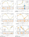 |
Fig. 1 Phase-folded RV curves for our six planets with the best-fit models. The color and filling of the points indicate the instrument used to acquire the data: empty blue for ELODIE, filled orange for SOPHIE, and empty orange for SOPHIE+. The error bars provided with the RV data are displayed with the same opacity and color as the points. The extended error bars computed with the fitted jitter parameters are displayed with a higher transparency. The best-fit model is represented with a greenline. The RV time series (not phase folded) are also displayed in Fig. B.1–B.4. |
4.6 HD 115954
For this system, we have 49 measurements: 4 from ELODIE, 6 from SOPHIE, 39 from SOPHIE+. The GLSP of the data (see Fig. B.4a) shows three peaks with an FAP lower than 0.1% around 0.5, 1 and 3000 days. We performed one exploration with 50 000 iterations per walker. It identified three local maxima. The difference of the logarithm of the posterior PDF values of the two lowest local maxima compared to the highest one are Δ ln (post) > 50. After selecting the global maximum and removing the burn-in phase, we obtained 1 175 000 converged iterations.
The best-fit Keplerian points toward a giant planet with a minimum mass of  Mjup, an orbital period of
  days and a significant eccentricity of
  . As for HD 27969 and HD 95544, the time span of the data covers just one orbital period, but this time a trend was initially observed in the residuals of the model, which led us to fit a linear trend to the data (see Table E.1 and Fig. B.4a). The fitted slope coefficient is not significant (see Table E.1), but displays a clear correlation with the orbital eccentricity and the RV offset between SOPHIE and SOPHIE+, and a slight correlation with the RV semi-amplitude. The dispersion of the residuals of the best-fit model is 7.5, 5.3, and 22.7 m s−1, which represents 1.6, 0.8, and 1.5 times the average error bar for SOPHIE+, SOPHIE and ELODIE, respectively. This indicates that there is probably no other significant signal in the data. The GLSP of the residuals (see Fig. B.4a) does not show any significant peak. The weighted average of the
  time series is −5.1 confirming that the star is quiet.
4.7 HD 211403
For this system, we have 52 measurements: 10 from ELODIE, 13 from SOPHIE, 29 from SOPHIE+. The GLSP of the data (see Fig. B.4b) shows three peaks with an FAP lower than 0.1% around 0.5, 1 and 220 days. We performed one exploration with 50 000 iterations per walker. It identified five local maxima. The difference of the logarithm of the posterior PDF values of the four lowest local maxima compared to the highest one are Δ ln (post) > 25. After selecting the global maximum and removing the burn-in phase, we obtained 375 000 converged iterations.
The best-fit Keplerian points toward a giant planet with a minimum mass of  Mjup, an orbital period of
  days and a low-significance eccentricity of
  . The time span of the observations covers around 23 orbital periods. No trend is observed in the residuals of the best-fit model (see Fig. B.4b). The dispersion of the residuals of the best-fit model is 35.9, 37.9 and 76.6 m s−1, which represents 1.9, 2.0, and 1.3 times the average error bar for SOPHIE+, SOPHIE, and ELODIE, respectively. This indicates that there is probably no other clearly significant signal in the data. The GLSP of the residuals (see Fig. B.4b) does not show any significant peak. The weighted average of the
  time series is −4.6, which indicates a relatively active star.
The estimated RV offset of − 219 m s−1 between the ELODIE and SOPHIE+ instruments is relatively large compared to the value obtained for HD 80869 and HD 115954 (see Table E.1). An abnormally high RV offset could be the sign of an RV drift and of an additional companion. We thus looked at the RV offset measurements published by Boisse et al. (2012) and Kiefer et al. (2019)8 to provide a broader context. In particular, Fig A.1 of Boisse et al. (2012) shows the RV offset between ELODIE and SOPHIE for a sample of stable stars. The authors showed that when using a G2 mask, as we do for HD 211403, the measured RV offset is typically in the range 0 to −120 m s−1. This RV offset could thus be the sign of an RV drift and of the presence of a companion at a larger orbital period.
4.8 Validation of the planetary nature
Periodic signals similar to the one produced by a planet orbiting the target star can be produced by spectroscopic binaries (SBs), contaminating spectroscopic binaries (CSBs), hierarchical triple systems (HTSs), and stellar activity (see for example Santerne et al. 2015; Queloz et al. 2001).
The first hypothesis to explore is the SB, where the system observed is composed of two stellar and gravitationally bound objects. As far as the identification of such systems is concerned, two cases need to be considered. The first case is the SB2. The magnitudes of both stars are sufficiently close to be able to observe two sets of lines in the observed spectra. A visual inspection of the spectrum also enables the detection of some cases of HTS and CSB, where the apparent magnitude of the target star is similar to that of one of the other stars involved in these scenarios. The inspection of our spectra enables us to reject these scenarios.
The second case is the SB1. In this scenario, the second star is too faint compared to the target star to enable the identification of two sets of lines. However, the gravitational pull of the stellar companion induces a large RV amplitude. The analysis of such systems under the planetary hypothesis, as performed in Sect. 4.1, leads to mass estimates that indicate a stellar companion. Assuming that the orbital inclination is not too low (the system is not face-on), the mass estimates provided in Table E.1 enable us to reject this hypothesis for most orbital inclinations.
99.7% confidence interval for the correlation coefficients between RV and BS, FWHM, and  .
.
4.8.1 False positive indicators
For the two remaining false positive cases, which imply a gravitationally bound system (i.e., HTS and CSB), the target star is not the one receiving the gravitational pull that we would detect. As shown by Santerne et al. (2015), the CCF of the star receiving the pull is blended with the one of the target star and deforms it. These deformations induce an RV signal when the CCF is fitted with a Gaussian profile. Such a scenario thus implies a deformation of the CCF profile, which can be captured by the BIS and FWHM of the CCF. If the detected RV variations originate from these deformations the RV will correlate with the BIS and/or the FWHM.
In Table 1, we present estimates of the correlation coefficient between the RV, BIS and FWHM for our six systems obtained with the method described in Figueira et al. (2016). All cases are compatible with no correlation (0) according to the 99.7% confidence interval, but two of them are not according to the 95% confidence interval (see the asterisks in Table 1). This analysis put some constraints on the CSB and HTS scenarios, but does not completely exclude them. It is indeed possible that the precision of the RV, BIS and FWHM measurements does not allow a significant detection of an existing correlation. Marginal detections (like the two that we mentioned) can be triggered due to the relatively small sample size (~ 25–60 measurements in these cases).
To address this point, we performed a simple dispersion analysis as described in Demangeon et al. (2018). It consists of computing the ratio of the dispersion over the average measurement error for the BIS and FWHM measurements (see results in Table 2). In short, in the CSB and HTS scenarios, because the RV signal is produced by the deformation of the CCF, both BIS and FWHM have to exhibit a dispersion whose amplitude is larger than their average error bar ( ). The values of
  for our data sets are provided in Table 2. If produced by a CSB or an HTS, this extra dispersion is equal to a fraction of the RV dispersion and should correlate with it. As described by Santerne et al. (2015), the value of this fraction depends on the characteristics of the CBS and HTS systems: magnitude ratio, mean RV separation, FWHM of the stellar components and spectral types. In Table 2, we also provide the maximum fraction of the RV dispersion that the FWHM or BIS can have without triggering a 3 sigma detection of an extra dispersion. This number allows us to understand how constraining this analysis is for each case. The dispersion analysis also complements the correlation analysis, since it accounts for measurement uncertainties. It indicates whether the dispersion of the measurements requires more than pure measurement uncertainty to be explained. If it is not the case, the correlation analysis cannot provide a reliable correlation detection. Marginal detections, like the two presented in Table 1, can then safely be ignored. If extra dispersion is detected, then the correlation analysis should be able to tell if it is correlated to the RV dispersion and thus if we can reject the planetary hypothesis in favor of the CSB or HTS hypothesis. Table 2 displays only one case, the FWHM of HD 109286,where the dispersion of the measurements cannot be explained solely by the measurement uncertainties:
  which is thus different from 1 at 4.3 sigma. As this extra dispersion does not correlate with the RV, we can still exclude the hypothesis that the source of this dispersion is also the source of the Keplerian-like signal observed in the RV and thus reject the CSB or HTS hypothesis. As we discuss in more detail in Sect. 4.8.3, the origin of this dispersion is probably stellar activity.
Analysis of the dispersion of the BIS and FWHM.
4.8.2 Astrometry
To investigate the CSB or HTS hypothesis even further, we inspected the Gaia Archive database9 (Gaia Collaboration 2016, 2018b) to find possible astrometric motions for these systems. The presence of an astrometric motion could show either an inclination different from edge-on or the presence of an unseen long-period companion (Kiefer et al. 2019; Kiefer 2019).
The six sources presented in this paper were all observed by the Gaia space telescope with data published in Data Release (DR) 1 and 2. Somewhat significant excess noise (>0.5 mas; Kiefer et al. 2019) was found in the DR1 for only two systems, HD 27969 (ϵDR1 = 0.62 mas) and HD 109286 (ϵDR1 = 0.88 mas). Nevertheless, these excess noises hardly stand out compared to the distribution of astrometric excess noise published in the DR1 for all primary sources monitored with Gaia, of which a majority are single stars, with a median at 0.45 mas and a 90th percentile at 0.85 mas. The excess noise measured for HD 109286 is slightly larger than this limit, and could therefore be real. Moreover, the instrumental and photon noise are minimized about the Gaia magnitude of this star G ~ 8.6 (Lindegren et al. 2018).
On the other hand, inspecting the DR2 archive, we did not find large deviations from a good astrometric fit with 5 parameters, with χ2 = 282 for 158 degrees of freedom. This is a reduced χ2 of 1.78, or a unit weight error UWE = 1.33. According to Lindegren et al. (2018), this is close to the median UWE at this magnitude of about 1.4. Therefore, no significant excess astrometric noise seems to be detected in DR2. If a (likely small) part of the DR1 excess noise measured for HD 109286 is real, then the fact it is not observed in DR2 implies that it could be due to an unseen long-period companion. The astrometric reflex motion of the star due to this companion may be partly fitted in DR2, which would not be the case in DR1. Indeed, the Tycho-2 and HIPPARCOS-2 positioning from 24 yr ago was taken into account in DR1 but not in DR2 (Lindegren et al. 2016, 2018). This hypothesis of an unseen long-period companion is reinforced by our detection of a linear RV trend (see Sect. 4.5).
We also examined the HIPPARCOS Intermediate Astrometry Data using the methods described in Sahlmann et al. (2016) to investigate whether they can put constraints on the systems’ parameters, and in particular on the masses of the companions. Table 3 lists the target names and the basic parameters of the HIPPARCOS observations relevant for the astrometric analysis. The solution type (Sol. Type) indicates the astrometric model adopted by the new reduction. For the standard five-parameter solution it is “5”. The parameter Norb represents the number of orbital periods covered by the HIPPARCOS observation time span. NHip is the number of astrometric measurements with a median precision of σλ. The last column in Table 3 shows the maximum companion mass (M2,max) that would be compatible with a non-detection in the HIPPARCOS astrometry. We do not detect significant orbital motion in the astrometry for any of these sources, but we determine upper mass limits of 0.14, 12.02, and 0.6 M⊙ for the companions of HD 27969, HD 109286, and HD 211403, respectively.
For our six targets, the Gaia and HIPPARCOS data thus agree with the planetary origin of the signal observed. They do not provide any indication that it could instead be produced by an SB, a CSB, or an HTS. Even if we cannot exclude all configurations of SB, CSB, or HTS, the simplest explanation is the planetary one. One false positive scenario, however, remains to be explored:stellar activity.
Parameters of the HIPPARCOS astrometric observations.
4.8.3 Investigating the stellar activity hypothesis
Stellar activity, in particular spots and plages, produces deformations of the CCF profile and intensity variations in stellar lines that are particularly sensitive to activity, like the flux variation at the core of the Ca II H&K lines measured by the  indicator (e.g., Duncan et al. 1991). It can thus produce quasi-periodic BIS, FWHM,
  and RV variations due to the intrinsic periodicity of the activity cycles or stellar rotation (e.g., Queloz et al. 2001). In such a case, we expect an extra dispersion in the FWHM and/or BIS and/or
  measurements, as observed for HD 109286 (see Table 2). If the signal observed in the RV data of HD 109286 was due to stellar activity, we would also expect a correlation between the FWHM and the RV measurements (e.g., Dumusque et al. 2014). This was not observed (see Table 1) for HD 109286 or any of other targets. This indicates that stellar activity is unlikely to be the source of the six RV signals that we detect. However, it could explain the extra dispersion of the FWHM detected in the data of HD 109286. This explanation is supported by the measurements of the
  , a well-known activity indicator (e.g., Wright et al. 2004). HD 109286 exhibits the highest
  with an average value of −4.45.
As the periods of the RV signals detected are quite large (from 224 to 3700 days), we must mention stellar magnetic cycles as another potential source of false positives. However, observations of RV signals associated with magnetic cycles have so far constrained their amplitude to a few tens of m s−1 (e.g., Gomes da Silva et al. 2012; Lovis et al. 2011), one order of magnitude smaller than any of the signals that we detect.
To confirm the rejection of the stellar activity hypothesis (whether coming from a magnetic cycle or not), in Appendix C, we show the GLSP of the BIS, FWHM and  time series (Fig. C.1–C.6). If the observed signals were due to stellar activity, we would expect to observe a peak at the same period in these GLSP s. This is not the case for any of our six planets. These GLSP could also show peaks at the stellar rotation period, but no significant peak (with FAP level below 10%) is observed in the any of BIS, FWHM or
  GLSP s for any of our six systems.
To conclude, the six periodic signals discovered in the RV observations of HD 27969, HD 80869, HD 95544, HD 109286, HD 115954 and HD 211403 are all of planetary origin to the best of our knowledge.
4.8.4 Search for additional planetary signals
Kima10 is a Python/C++ open-source package developed for the detection of exoplanets with RV data (Faria et al. 2018). It makes use of the diffusive nested sampling algorithm (Brewer et al. 2011) to infer the number of planets present in a set of RV measurements. To do this, kima calculates the evidence for a model with a given number of planets (Np). In our work Np is set as a free parameter between 0 and 2, and we evaluate the posterior distribution for Np to determine the number of planets detected. This means that to claim the detection of Np planets, the probability of Np planets needs to be at least 150 times greater than the probability of Np-1 planets (Kass & Raftery 1995).
The analyses of the RV series of our six targets conclude that in all cases the best model is a model with only one planet. Such a confirmation is particularly important for planets with high orbital eccentricity. A highly eccentric orbit can indeed mimic the signal from two planets on close to circular orbits (Wittenmyer et al. 2019a, 2013).
Furthermore, for HD 109286 and HD 115954, our model also included an RV trend that could be due to an additional body with an even longer orbital period (e.g., Wittenmyer et al. 2019b) in the system, or to stellar activity (like the signature of a magnetic cycle). Finally, Kima also provides the parameters of the detected planets. All parameters are compatible within 1 sigma with the ones obtained by the analysis described in Sect. 4.1.
5 Discussion
In this paper we have presented the detection of six giant planets with minimum masses ranging from 2.99 to 8.29 Mjup and long orbital periods ranging from 223.7 to 3700 days (~10 yr). We now discuss the importance of these planets in the context of the known exoplanet population.
5.1 The importance of the cold and eccentric giant planet population
Figure 2 presents our six planets in the mass-period-eccentricity diagram along with the known exoplanet population. Our six planets belong to a relatively populated part of the distribution: the cold giant planets. According to NASA Exoplanet Archive (Akeson et al. 2013), we currently know of 354 planets with a mass larger than 0.2 Mjup and an orbital period above 100 days11. Within this population, HD 80869 b stands out as the planet with the seventh most eccentric orbit12, and HD 115954 b and HD 109286 b also have eccentricities above the median eccentricity (0.198) of the known exoplanet population13.
Reaching a statistical understanding of the eccentricity distribution of the exoplanet population, and in particular its high tail, is essential for constraining planetary formation and migration models (e.g., Chatterjee et al. 2008; Jurić & Tremaine 2008; Bowler et al. 2020). Eccentric planets are not a direct output of planet formation from core-accretion in a protoplanetary disk (see for example Lin & Ida 1997). The interaction between the planet and the disk usually damps the eccentricity. Eccentric orbits thus require an additional process. Three such processes are discussed in the literature: disk cavity migration, planet-planet scattering, and Kozai-Lidov perturbations. Disk cavity migration (e.g., Goldreich & Sari 2003; Debras et al. 2021) is a special case of giant planet-disk tidal interaction that promotes eccentricity growth instead of damping it. Eccentricity damping relies on the balance between waves produced by two kinds of resonances: the Lindblad resonances, which excite the eccentricity, and the corotation resonances, which damp it (e.g., Papaloizou et al. 2001). When a planet is more massive than ~ 10Mjup, it opens a cavity in the disk. If this cavity is wide enough to encompass the principal Lindblad resonances and the first-order corotation resonances, the planet’s eccentricity is controlled by the next most important resonances: the first-order Lindblad resonances. This process can explain eccentricities of up to ~ 0.4. The planet-planet scattering scenario (Rasio & Ford 1996; Weidenschilling & Marzari 1996; Lin & Ida 1997) relies on close encounters between two planets. The gravitational interaction between the two bodies can send them into eccentric orbits. If such an event arises after the dissipation of the protoplanetary disk, and the eccentric orbit does not trigger other close encounters with other planets or efficient tidal dissipation with the parent star, the planet can remain on its eccentric orbit. The Kozai-Lidov perturbation (Kozai 1962; Lidov 1962) also requires the presence of another massive body, a star or a massive substellar companion, but this time not located in the plane of the protoplanetary disk. In such a case, the difference of orbital inclination between the planet and this third body can excite both the orbital inclination and the eccentricity of the planet. These last two scenarios are often used to explain the existence of hot Jupiters (see for example Winter et al. 2020; Teyssandier et al. 2019). Hot Jupiters would represent the fraction of eccentric giant planets whose eccentricity led to strong tidal interactions with the parent star, a dissipation of the angular momentum, and a circularization of the planet’s orbit (e.g., Ogilvie 2014). The process or processes that explain the presence and characteristics of hot Jupiters must also explain the properties of the eccentric cold Jupiter population to which several of our newly discovered planets belong.
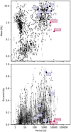 |
Fig. 2 Mass versus orbital period distribution (top) and orbital eccentricity versus orbital period distribution (bottom) of the known exoplanet population according to NASA Exoplanet Archive. We only display exoplanets with a relative mass and orbital period precision better than 50%. The six exoplanets announced in this paper are marked in blue with a thick circle, and the last three digits of their host star names are displayed (for example “869” for HD 80869 b). The red stars indicate Solar System planets for reference. |
5.2 The small planet-cold Jupiter relation
A large fraction of the known planets belong to multiple systems14, and it is not rare for an apparently single-planet system to actually harbor other undetected planets (Sandford et al. 2019). We have seen that our data sets do not support the presence of additional planets in any of our six systems (Sect. 4.8.4). However, the observational strategy of our RV program is not favorable to multi-planetary system discoveries. The low cadence and relatively low RV precision of our data sets are well adapted for the detection of cold Jupiters, but not for the detection of super-Earths or sub-Neptunes on shorter orbits.
From the analysis of planets detected with both RV and transit photometry surveys, Zhu & Wu (2018) showed that there is a correlation between the presence of small short-period planets (planets with mass and radius between those of Earth and Neptune) and the presence of giant long-period15 planets within the same system. More specifically, they conclude that cold Jupiters are almost certainly (~ 90%) accompanied by small planets. These results are in agreement with other independent studies (Bryan et al. 2016, 2019) and indicate that our six stars are likely to host small planets that are undetected in our data sets. Three out of the six cold Jupiters discussed in this paper have an orbital eccentricity higher than 0.3. We can expect a cold Jupiter with a high orbital eccentricity to compromise the stability of the inner planetary system and impact the probability of finding a small inner planet (Pu & Lai 2018; Mustill et al. 2017). It is relevant at this point to mention that there is currently only one system known to host at least one small inner planet and a cold Jupiter with an orbital eccentricity above 0.8 (Santos et al. 2016). It is thus not common, but also not impossible, for a system hosting a cold Jupiter with such a highly eccentric orbit to host a small inner planet. Zhu & Wu (2018) did not directly study this question, but they approached it indirectly by comparing the multiplicity of inner-planetary systems with and without a known cold Jupiter. As cold Jupiters are known to have eccentric orbits (see for example Fig. 2 of Zhu & Wu 2018), if the presence of a cold Jupiter reduces the multiplicity of small inner planetary systems, the eccentricity of the orbit of the cold Jupiter can be proposed as an explanation, even if it is not the only possible explanation. In their sample, Zhu & Wu (2018) found that the average number of small inner planets is 2.5 for systems without a cold Jupiter and drops to 1.4 for systems that also host a cold Jupiter.
We will thus follow up on these six stars with a higher cadence and a higher RV precision to detect additional small planets in these systems.
Acknowledgements
O.D.S.D. is supported in the form of work contract (DL 57/2016/CP1364/CT0004) funded by national funds through Fundação para a Ciência e a Tecnologia (FCT). This work was supported by Fundação para a Ciência e a Tecnologia (FCT) and Fundo Europeu de Desenvolvimento Regional (FEDER) via COMPETE2020 through the research grants UIDB/04434/2020, UIDP/04434/2020, PTDC/FIS-AST/32113/2017 & POCI-01-0145-FEDER-032113, PTDC/FIS-AST/28953/2017 & POCI-01-0145-FEDER-028953. This work has been carried out in part within the framework of the NCCR PlanetS supported by the Swiss National Science Foundation. This project has received funding from the European Research Council (ERC) under the European Union’s Horizon 2020 research and innovation programme (project SPICE DUNE; grant agreement No 947634). I.B., G.H, and X.D. received funding from the French Programme National de Physique Stellaire (PNPS) and the Programme National de Planétologie (PNP) of CNRS (INSU). B.N. acknowledges postdoctoral funding from the Alexander von Humboldt Foundation. T.L.C. is also supported by FCT in the form of a work contract (CEECIND/00476/2018). M.J.H. acknowledges support from ANID - Millennium Science Initiative - ICN12 009. B.N. acknowledges postdoctoral funding from the Alexander von Humboldt Foundation and “Branco Weiss fellowship Science in Society” through the SEISMIC stellar interior physics group. This work made use of Simbad, Vizier and exoplanet.eu. Most of the analyses presented in this paper were performed using the Python language (version 3.5) available at http://www.python.org and several scientific packages: Numpy (van der Walt et al. 2011), Scipy (Virtanen et al. 2020), Pandas (McKinney 2010), Ipython (Pérez & Granger 2007), Astropy (Astropy Collaboration 2013, 2018) and Matplotlib (Hunter 2007).
Appendix A Prior distributions
Table A.1 lists the priors used for all the parameters of the model in the Bayesian analysis. P and tic on one side and e cos ω* and e sin ω* on the other are affect joint prior probabilities. P and tic are affected by the joint prior  . In practice, this means that P and tic are used to compute the phase of inferior conjunction ϕic defined as
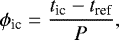
where tref is defined as the time of the first measurement obtained with SOPHIE+ floored to the closest integer. Then individual priors are affected to P and ϕic : A Jeffreys prior between 0.1 day and 1.5 times the time span of the observations for P and a uniform prior between 0 and 1 for ϕic. The joint prior on P and tic can thus be written as
Here, e cos ω* and e sin ω* are affected by the joint prior  . This means that we compute the eccentricity (e) and the argument of periastron of the stellar orbit (ω*) and affect a beta prior with shape parameters a and b equal to 0.867 and 3.03, respectively, to e (as suggested by Kipping 2013), and a uniform prior between − π and π to ω*. The joint prior on e cos ω* and e sin ω* can thus be written as

Priors of Bayesian MCMC analysis.
Appendix B RV time series and generalized Lomb-Scargle periodograms
We show in Figs. B.1–B.4 the RV time series and the GLSP of the RV data, the planetary model, the residuals and the window function. These figures allow a visual assessment of the quality of the fitted model and the presence of trends and additional signals in the residuals.
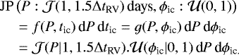
 |
Fig. B.1 Radial velocities, best-fit model, and residuals for the HD27969 system. Left-top: RV time series and best-fit model, from which the systemic velocity and the offsets between instruments have been removed. Left-bottom: time series of the residuals of the best-fit model. The color and filling of the points indicate the instrument used to acquire the data: empty blue for ELODIE, filled orange for SOPHIE, and empty orange for SOPHIE+. The error bars provided with the RV data are displayed with the same opacity and color as the points. The extended error bars computed with the fitted additive jitter parameters are displayed with a higher transparency. Middle, top: GLSP of the RV time series, the best-fit model sampled at the same times as the RV s (middle, second from the top), the residuals (middle, third from top), and the window function (middle, bottom). Right: GLSP s zoomed-in around the period of the detected planet. The best-fit orbital period of the planet is marked by a vertical dashed red line. The horizontal dotted, dash-dotted, and dashed black lines correspond to 0.1, 1, and 10% FAP (Zechmeister & Kürster 2009) levels, respectively. |
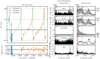 |
Fig. B.2 Radial velocities, best-fit model, and residuals for the HD 80869 system. This figure is structured and generated in the same way as Fig. B.1 (see the caption of that figure for more details). The main difference is that in this case we add, in the third row, the GLSP of the planetary model sampled at 10 000 times, evenly spread over the time span of our observations (modelHS). This allows us to visualize the harmonic content of this highly eccentric orbit and better understand the GLSP of our RV data. |
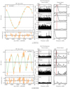 |
Fig. B.3 Radial velocities, best-fit model, and residuals for the HD 95544 (a) and HD 109286 (b) systems. This figure is structured and generated in the exact same way as Fig. B.1 (see the caption of that figure for more details). |
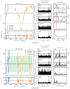 |
Fig. B.4 Radial velocities, best-fit model, and residuals for the HD 115954 (a) and HD 211403 (b) systems. This figure is structured and generated in the exact same way as Fig. B.1 (see the caption of that figure for more details). |
Appendix C GLSP of the activity indicators
Figures C.1 to C.6 show the GLSP of the RV, FWHM, BIS and  data collected forour six systems and their associated window function. The frequency and period ranges are chosen to visualize the region surrounding the observed planetary periods and check that the GLSP of the FWHM, BIS and
  data do not showa significant peak at the same period. These frequency and period ranges are not always suited to visualizing shorter periods and assessing the presence of peaks associated with the stellar rotation period. However, we inspected these GLSP at shorter periods and do not report any peak with FAP levels below 10%.
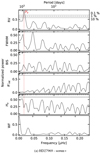 |
Fig. C.1 GLSP of the RV and the available activity indicators measured on HD 27969 with the SOPHIE (SOPHIE+) spectrograph. From top to bottom: GLSP of the RV, FWHM, BIS, and |

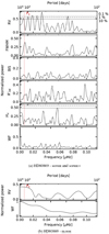 |
Fig. C.2 GLSP of the RV and the available activity indicators measured on HD 80869 with the SOPHIE (SOPHIE and SOPHIE+) spectrograph (a) and the ELODIE spectrograph (b). (a) From top to bottom: GLSP of the RV, FWHM, BIS, and
|


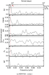 |
Fig. C.3 GLSP of the RV and the available activity indicators measured on HD 95544 with the SOPHIE (SOPHIE+) spectrograph. From top to bottom: GLSP of the RV, FWHM, BIS, and
|

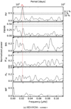 |
Fig. C.4 GLSP of the RV and the available activity indicators measured on HD 109286 with the SOPHIE (SOPHIE+) spectrograph. From top to bottom: GLSP of the RV, FWHM, BIS, and
|

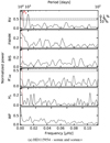 |
Fig. C.5 GLSP of the RV and the available activity indicators measured on HD 115954 with the SOPHIE (SOPHIE and SOPHIE+) spectrograph. From top to bottom: GLSP of the RV, FWHM, BIS, and
|

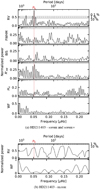 |
Fig. C.6 GLSP of the RV and the available activity indicators measured on HD211403 with the SOPHIE (SOPHIE and SOPHIE+) spectrograph (a) and the ELODIE spectrograph (b). (a) From top to bottom: GLSP of the RV, FWHM, BIS, and
|


Appendix D Radial velocities, FWHM, BIS, and log R’HK
Tables D.1 to D.6 provide the RV, FWHM, BIS,  and Hα measurements obtained forour six stars. For ELODIE data, we only derive RV. We provide error bars for the RV,
  and Hα measurements. Following Santerne et al. (2015), the uncertainties on the FWHM and BIS measurements can be obtained by multiplying the RV uncertainties by a factor of 2.5.
RV, FWHM, BIS,  , and Hα for star HD 27969.
RV, FWHM, BIS,  , and Hα for star HD 80869.
RV, FWHM, BIS,  , and Hα for star HD 95544.
RV, FWHM, BIS,  , and Hα for star HD 109286.
RV, FWHM, BIS,  , and Hα for star HD 115954.
RV, FWHM, BIS,  , and Hα for star HD 211403.
Appendix E Additional table
System parameters from Bayesian MCMC analysis.
References
- Akeson, R. L., Chen, X., Ciardi, D., et al. 2013, PASP, 125, 989 [NASA ADS] [CrossRef] [Google Scholar]
- Anderson, E., & Francis, C. 2011, VizieR Online Data Catalog: V/137B [Google Scholar]
- Astropy Collaboration (Robitaille, T. P., et al.) 2013, A&A, 558, A33 [NASA ADS] [CrossRef] [EDP Sciences] [Google Scholar]
- Astropy Collaboration (Price-Whelan, A. M., et al.) 2018, AJ, 156, 123 [Google Scholar]
- Bailer-Jones, C. A. L. 2011, MNRAS, 411, 435 [NASA ADS] [CrossRef] [Google Scholar]
- Baluev, R. V. 2009, MNRAS, 393, 969 [NASA ADS] [CrossRef] [Google Scholar]
- Baranne, A., Queloz, D., Mayor, M., et al. 1996, A&AS, 119, 373 [NASA ADS] [CrossRef] [EDP Sciences] [Google Scholar]
- Bergmann, C., Jones, M. I., Zhao, J., et al. 2021, PASA, 38, 15 [CrossRef] [Google Scholar]
- Boisse, I., Eggenberger, A., Santos, N. C., et al. 2010, A&A, 523, A88 [NASA ADS] [CrossRef] [EDP Sciences] [Google Scholar]
- Boisse, I., Bouchy, F., Hébrard, G., et al. 2011, A&A, 528, A4 [NASA ADS] [CrossRef] [EDP Sciences] [Google Scholar]
- Boisse, I., Pepe, F., Perrier, C., et al. 2012, A&A, 545, A55 [NASA ADS] [CrossRef] [EDP Sciences] [Google Scholar]
- Bonomo, A. S., Santerne, A., Alonso, R., et al. 2010, A&A, 520, A65 [NASA ADS] [CrossRef] [EDP Sciences] [Google Scholar]
- Borucki, W. J., Koch, D., Basri, G., et al. 2010, Science, 327, 977 [NASA ADS] [CrossRef] [PubMed] [Google Scholar]
- Bouchy, F., Hébrard, G., Udry, S., et al. 2009, A&A, 505, 853 [NASA ADS] [CrossRef] [EDP Sciences] [Google Scholar]
- Bouchy, F., Díaz, R. F., Hébrard, G., et al. 2013, A&A, 549, A49 [NASA ADS] [CrossRef] [EDP Sciences] [Google Scholar]
- Bovy, J., Rix, H.-W., Green, G. M., Schlafly, E. F., & Finkbeiner, D. P. 2016, ApJ, 818, 130 [NASA ADS] [CrossRef] [Google Scholar]
- Bowler, B. P. 2016, PASP, 128, 102001 [NASA ADS] [CrossRef] [Google Scholar]
- Bowler, B. P., Blunt, S. C., & Nielsen, E. L. 2020, AJ, 159, id.63 [NASA ADS] [CrossRef] [Google Scholar]
- Brewer, B. J., Pártay, L. B., & Csányi, G. 2011, Stat. Comput., 21, 649 [Google Scholar]
- Bryan, M. L., Knutson, H. A., Howard, A. W., et al. 2016, ApJ, 821, 89 [NASA ADS] [CrossRef] [Google Scholar]
- Bryan, M. L., Knutson, H. A., Lee, E. J., et al. 2019, AJ, 157, 52 [Google Scholar]
- Chatterjee, S., Ford, E. B., Matsumura, S., & Rasio, F. A. 2008, ApJ, 686, 580 [NASA ADS] [CrossRef] [Google Scholar]
- Cumming, A., Butler, R. P., Marcy, G. W., et al. 2008, PASP, 120, 531 [CrossRef] [Google Scholar]
- Dalba, P. A., Kane, S. R., Isaacson, H., et al. 2021, AJ, 161, 103 [NASA ADS] [CrossRef] [Google Scholar]
- Debras, F., Baruteau, C., & Donati, J.-F. 2021, MNRAS, 500, 1621 [Google Scholar]
- Demangeon, O. D. S., Faedi, F., Hébrard, G., et al. 2018, A&A, 610, A63 [CrossRef] [EDP Sciences] [Google Scholar]
- Díaz, R. F., Rey, J., Demangeon, O., et al. 2016, A&A, 591, A146 [NASA ADS] [CrossRef] [EDP Sciences] [Google Scholar]
- Dumusque, X., Boisse, I., & Santos, N. C. 2014, ApJ, 796, 132 [NASA ADS] [CrossRef] [Google Scholar]
- Duncan, D. K., Vaughan, A. H., Wilson, O. C., et al. 1991, ApJS, 76, 383 [NASA ADS] [CrossRef] [Google Scholar]
- Eastman, J., Gaudi, B. S., & Agol, E. 2013, PASP, 125, 83 [NASA ADS] [CrossRef] [Google Scholar]
- Faria, J. P., Santos, N. C., Figueira, P., & Brewer, B. J. 2018, J. Open Source Softw., 3, 487 [NASA ADS] [CrossRef] [Google Scholar]
- Fernandes, R. B., Mulders, G. D., Pascucci, I., Mordasini, C., & Emsenhuber, A. 2019, ApJ, 874, 81 [NASA ADS] [CrossRef] [Google Scholar]
- Figueira, P., Faria, J. P., Adibekyan, V. Z., Oshagh, M., & Santos, N. C. 2016, Origins Life Evol. Biosph., 46, 385 [NASA ADS] [CrossRef] [Google Scholar]
- Flower, P. J. 1996, ApJ, 469, 355 [NASA ADS] [CrossRef] [Google Scholar]
- Foreman-Mackey, D., Hogg, D. W., Lang, D., & Goodman, J. 2013, PASP, 125, 306 [Google Scholar]
- Foreman-Mackey, D., Morton, T. D., Hogg, D. W., Agol, E., & Schölkopf, B. 2016, AJ, 152, 206 [NASA ADS] [CrossRef] [Google Scholar]
- Fulton, B. J., Petigura, E. A., Blunt, S., & Sinukoff, E. 2018, PASP, 130, 044504 [NASA ADS] [CrossRef] [Google Scholar]
- Gaia Collaboration (Prusti, T., et al.) 2016, A&A, 595, A1 [NASA ADS] [CrossRef] [EDP Sciences] [Google Scholar]
- Gaia Collaboration 2018a, VizieR Online Data Catalog: I/345 [Google Scholar]
- Gaia Collaboration (Brown, A. G. A., et al.) 2018b, A&A, 616, A1 [NASA ADS] [CrossRef] [EDP Sciences] [Google Scholar]
- Gaia Collaboration (Mignard, F., et al.) 2018c, A&A, 616, A14 [NASA ADS] [CrossRef] [EDP Sciences] [Google Scholar]
- Geweke, J. 1992, Bayesian Stat., 4, 641 [Google Scholar]
- Goldreich, P., & Sari, R. 2003, ApJ, 585, 1024 [Google Scholar]
- Gomes da Silva, J., Santos, N. C., Bonfils, X., et al. 2012, A&A, 541, A9 [NASA ADS] [CrossRef] [EDP Sciences] [Google Scholar]
- Gregory, P. C. 2005, Bayesian Logical Data Analysis for the Physical Sciences: a Comparative Approach with Mathematica Support, ed. P. C. Gregory (Cambridge: Cambridge University Press) [Google Scholar]
- Hébrard, G., Bouchy, F., Pont, F., et al. 2008, A&A, 488, 763 [NASA ADS] [CrossRef] [EDP Sciences] [Google Scholar]
- Hébrard, G., Arnold, L., Forveille, T., et al. 2016, A&A, 588, A145 [NASA ADS] [CrossRef] [EDP Sciences] [Google Scholar]
- Hsu, D. C., Ford, E. B., Ragozzine, D., & Ashby, K. 2019, AJ, 158, 109 [NASA ADS] [CrossRef] [Google Scholar]
- Hunter, J. D. 2007, Comput. Sci. Eng., 9, 90 [NASA ADS] [CrossRef] [Google Scholar]
- Ida, S., Tanaka, H., Johansen, A., Kanagawa, K. D., & Tanigawa, T. 2018, ApJ, 864, 77 [NASA ADS] [CrossRef] [Google Scholar]
- Jeffreys, H. 1998, The Theory of Probability (Oxford: Oxford University Press) [Google Scholar]
- Jennings, J., Ercolano, B., & Rosotti, G. P. 2018, MNRAS, 477, 4131 [NASA ADS] [CrossRef] [Google Scholar]
- Jurić, M., & Tremaine, S. 2008, ApJ, 686, 603 [Google Scholar]
- Kass, R. E., & Raftery, A. E. 1995, J. Am. Stat. Assoc., 90, 773 [CrossRef] [Google Scholar]
- Kiefer, F. 2019, A&A, 632, L9 [CrossRef] [EDP Sciences] [Google Scholar]
- Kiefer, F., Hébrard, G., Sahlmann, J., et al. 2019, A&A, 631, A125 [NASA ADS] [CrossRef] [EDP Sciences] [Google Scholar]
- Kipping, D. M. 2013, MNRAS, 434, L51 [NASA ADS] [CrossRef] [Google Scholar]
- Kozai, Y. 1962, AJ, 67, 591 [Google Scholar]
- Kurucz, R. 1993, ATLAS9 Stellar Atmosphere Programs and 2 km/s grid. Kurucz CD-ROM No. 13. Cambridge (Mass.: Smithsonian Astrophysical Observatory), 13 [Google Scholar]
- Lammer, H., Brasser, R., Johansen, A., Scherf, M., & Leitzinger, M. 2021, Space Sci. Rev., 217, 7 [NASA ADS] [CrossRef] [Google Scholar]
- Levison, H., & Agnor, C. 2003, EGS - AGU - EUG Joint Assembly, 3917 [Google Scholar]
- Lidov, M. L. 1962, Planet. Space Sci., 9, 719 [Google Scholar]
- Lin, D. N. C., & Ida, S. 1997, ApJ, 477, 781 [NASA ADS] [CrossRef] [Google Scholar]
- Lindegren, L., Lammers, U., Bastian, U., et al. 2016, A&A, 595, A4 [NASA ADS] [CrossRef] [EDP Sciences] [Google Scholar]
- Lindegren, L., Hernández, J., Bombrun, A., et al. 2018, A&A, 616, A2 [NASA ADS] [CrossRef] [EDP Sciences] [Google Scholar]
- Lovis, C., & Fischer, D. 2010, Exoplanets (Washington, DC: Smithsonian Books), 27 [Google Scholar]
- Lovis, C., Dumusque, X., Santos, N. C., et al. 2011, ArXiv e-prints [arXiv:1107.5325] [Google Scholar]
- Mayor, M., & Queloz, D. 1995, Nature, 378, 355 [Google Scholar]
- Mayor, M., Marmier, M., Lovis, C., et al. 2011, ArXiv eprints [arXiv:1109.2497] [Google Scholar]
- McKinney, W. 2010, in Proceedings of the 9th Python in Science Conference (Stéfan van der Walt and Jarrod Millman), 51–56 [Google Scholar]
- Morbidelli, A., Lunine, J. I., O’Brien, D. P., Raymond, S. N., & Walsh, K. J. 2012, Ann. Rev. Earth Planet. Sci., 40, 251 [NASA ADS] [CrossRef] [Google Scholar]
- Mordasini, C. 2018, Handbook of Exoplanets (Berlin: Springer), 143 [Google Scholar]
- Moutou, C., Hébrard, G., Bouchy, F., et al. 2014, A&A, 563, A22 [NASA ADS] [CrossRef] [EDP Sciences] [Google Scholar]
- Mustill, A. J., Davies, M. B., & Johansen, A. 2017, MNRAS, 468, 3000 [Google Scholar]
- Nsamba, B., Campante, T. L., Monteiro, M. J. P. F. G., et al. 2018, MNRAS, 477, 5052 [NASA ADS] [CrossRef] [Google Scholar]
- Ogilvie, G. I. 2014, ARA&A, 52, 171 [Google Scholar]
- Papaloizou, J. C. B., Nelson, R. P., & Masset, F. 2001, A&A, 366, 263 [NASA ADS] [CrossRef] [EDP Sciences] [Google Scholar]
- Pascucci, I., Gorti, U., Hollenbach, D., et al. 2006, ApJ, 651, 1177 [CrossRef] [Google Scholar]
- Paxton, B., Cantiello, M., Arras, P., et al. 2013, ApJS, 208, 4 [NASA ADS] [CrossRef] [Google Scholar]
- Paxton, B., Marchant, P., Schwab, J., et al. 2015, ApJS, 220, 15 [Google Scholar]
- Paxton, B., Schwab, J., Bauer, E. B., et al. 2018, ApJS, 234, 34 [NASA ADS] [CrossRef] [EDP Sciences] [Google Scholar]
- Pecaut, M. J.,& Mamajek, E. E. 2013, ApJS, 208, 9 [NASA ADS] [CrossRef] [Google Scholar]
- Pepe, F., Mayor, M., Galland, F., et al. 2002, A&A, 388, 632 [NASA ADS] [CrossRef] [EDP Sciences] [Google Scholar]
- Pérez, F., & Granger, B. E. 2007, Comput. Sci. Eng., 9, 21 [Google Scholar]
- Perruchot, S., Kohler, D., Bouchy, F., et al. 2008, SPIE, 7014, 70140J [NASA ADS] [Google Scholar]
- Pijpers, F. P. 2003, A&A, 400, 241 [NASA ADS] [CrossRef] [EDP Sciences] [Google Scholar]
- Pu, B., & Lai, D. 2018, MNRAS, 478, 197 [NASA ADS] [CrossRef] [Google Scholar]
- Queloz, D., Henry, G. W., Sivan, J. P., et al. 2001, A&A, 379, 279 [NASA ADS] [CrossRef] [EDP Sciences] [Google Scholar]
- Rasio, F. A., & Ford, E. B. 1996, Science, 274, 954 [NASA ADS] [CrossRef] [PubMed] [Google Scholar]
- Raymond, S. N., Quinn, T., & Lunine, J. I. 2005, ApJ, 632, 670 [NASA ADS] [CrossRef] [Google Scholar]
- Rendle, B. M., Buldgen, G., Miglio, A., et al. 2019, MNRAS, 484, 771 [Google Scholar]
- Sahlmann, J., Lazorenko, P. F., Ségransan, D., et al. 2016, A&A, 595, A77 [NASA ADS] [CrossRef] [EDP Sciences] [Google Scholar]
- Sandford, E., Kipping, D., & Collins, M. 2019, MNRAS, 489, 3162 [Google Scholar]
- Santerne, A., Díaz, R. F., Almenara, J.-M., et al. 2015, MNRAS, 451, 2337 [NASA ADS] [CrossRef] [Google Scholar]
- Santos, N. C., Sousa, S. G., Mortier, A., et al. 2013, A&A, 556, A150 [NASA ADS] [CrossRef] [EDP Sciences] [Google Scholar]
- Santos, N. C., Santerne, A., Faria, J. P., et al. 2016, A&A, 592, A13 [NASA ADS] [CrossRef] [EDP Sciences] [Google Scholar]
- Sneden, C. 1973, ApJ, 184, 839 [Google Scholar]
- Sousa, S. G. 2014, Determination of Atmospheric Parameters of B-, A-, F- and G-Type Stars, Series: GeoPlanet: Earth and Planetary Sciences, eds. E. Niemczura, B. Smalley, & W. Pych (Cham: Springer), 297 [CrossRef] [Google Scholar]
- Sousa, S. G., Santos, N. C., Israelian, G., Mayor, M., & Monteiro, M. J. P. F. G. 2007, A&A, 469, 783 [NASA ADS] [CrossRef] [EDP Sciences] [Google Scholar]
- Sousa, S. G., Santos, N. C., Mayor, M., et al. 2008, A&A, 487, 373 [NASA ADS] [CrossRef] [EDP Sciences] [MathSciNet] [Google Scholar]
- Sousa, S. G., Santos, N. C., Adibekyan, V., Delgado-Mena, E., & Israelian, G. 2015, A&A, 577, A67 [NASA ADS] [CrossRef] [EDP Sciences] [Google Scholar]
- Sousa, S. G., Adibekyan, V., Delgado-Mena, E., et al. 2018, A&A, 620, A58 [NASA ADS] [CrossRef] [EDP Sciences] [Google Scholar]
- Teyssandier, J., Lai, D., & Vick, M. 2019, MNRAS, 486, 2265 [NASA ADS] [CrossRef] [Google Scholar]
- Thompson, S. E., Coughlin, J. L., Hoffman, K., et al. 2018, ApJS, 235, 38 [NASA ADS] [CrossRef] [Google Scholar]
- Torres, G. 2010, AJ, 140, 1158 [NASA ADS] [CrossRef] [Google Scholar]
- Torres, G., Fischer, D. A., Sozzetti, A., et al. 2012, ApJ, 757, 161 [Google Scholar]
- Tsantaki, M., Sousa, S. G., Adibekyan, V. Z., et al. 2013, A&A, 555, A150 [NASA ADS] [CrossRef] [EDP Sciences] [Google Scholar]
- Tsantaki, M., Sousa, S. G., Santos, N. C., et al. 2014, A&A, 570, A80 [NASA ADS] [CrossRef] [EDP Sciences] [Google Scholar]
- Valenti, J. A., & Piskunov, N. 1996, A&AS, 118, 595 [NASA ADS] [CrossRef] [EDP Sciences] [Google Scholar]
- van der Walt, S., Colbert, S. C., & Varoquaux, G. 2011, Comput. Sci. Eng., 13, 22 [Google Scholar]
- Virtanen, P., Gommers, R., Oliphant, T. E., et al. 2020, Nat. Methods, 17, 261 [Google Scholar]
- Weidenschilling, S. J., & Marzari, F. 1996, Nature, 384, 619 [Google Scholar]
- Winter, A. J., Kruijssen, J. M. D., Longmore, S. N., & Chevance, M. 2020, Nature, 586, 528 [Google Scholar]
- Wittenmyer, R. A., Wang, S., Horner, J., et al. 2013, ApJS, 208, 2 [NASA ADS] [CrossRef] [Google Scholar]
- Wittenmyer, R. A., Butler, R. P., Tinney, C. G., et al. 2016, ApJ, 819, 28 [NASA ADS] [CrossRef] [Google Scholar]
- Wittenmyer, R. A., Bergmann, C., Horner, J., Clark, J., & Kane, S. R. 2019a, MNRAS, 484, 4230 [NASA ADS] [CrossRef] [Google Scholar]
- Wittenmyer, R. A., Clark, J. T., Zhao, J., et al. 2019b, MNRAS, 484, 5859 [NASA ADS] [CrossRef] [Google Scholar]
- Wright, J. T., Marcy, G. W., Butler, R. P., & Vogt, S. S. 2004, ApJS, 152, 261 [NASA ADS] [CrossRef] [Google Scholar]
- Zechmeister, M., & Kürster, M. 2009, A&A, 496, 577 [NASA ADS] [CrossRef] [EDP Sciences] [Google Scholar]
- Zhu, W., & Wu, Y. 2018, AJ, 156, 92 [NASA ADS] [CrossRef] [Google Scholar]
The planet candidates discovered by the Kepler mission are available at the NASA Exoplanet Archive.
Fernandes et al. (2019) defined cold Jupiters as planets with a mass or a minimum mass in the range of 0.1–20 Mjup and a semimajor axis between 0.1 and 100 au.
Several of the Python packages used for this work are publicly available on Github: radvel at https://github.com/California-Planet-Search/radvel, emcee at https://github.com/dfm/emcee
Quantitatively, the walkers that belong to the highest peak are defined as all walkers whose highest posterior values satisfy this criterion:
 where
where
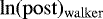 is the natural logarithm of the highest posterior value identified by a walker,
  is the maximum of the logarithm of the posterior identified by all walkers and MAD is the median absolute deviation. We visually confirmed that this criterion corresponds to a peak in the histogram of
 .
.
In our analysis the typical correlation length of the chain is between 5 and 20, which means that we have 5–20 times fewer independent samples.
The FAP levels are computed using the analytical relation described in Zechmeister & Kürster (2009) when the Z-K normalization is used.
We want to caution the reader interested in the RV offset between ELODIE and SOPHIE. Kiefer et al. (2019) mentioned that the expected range is between 50 and 100 m s−1 according to Bouchy et al. (2013). This reference is probably erroneous and should be Boisse et al. (2012). Furthermore, the 50–100 m s−1 range is valid only for RV s computed with a G2 mask.
On top of the mass and period lower limits provided, we only considered exoplanets whose mass and orbital period are measured with a relative precision better than 50%.
According to the NASA exoplanet archive, HD 80869 b is the planet with the sixth most eccentric orbit, but the archive does not yet take into account the recently updated orbital parameters of HD 76920 b (Bergmann et al. 2021).
We again only considered planets whose mass and orbital period are measured with a relative precision better than 50%.
According to NASA exoplanet archive, currently 43% of the known planets belong to a multiple system.
Zhu & Wu (2018) define a “long period” as an orbital period above one year.
All Tables
99.7% confidence interval for the correlation coefficients between RV and BS, FWHM, and .
All Figures
|
Fig. 1 Phase-folded RV curves for our six planets with the best-fit models. The color and filling of the points indicate the instrument used to acquire the data: empty blue for ELODIE, filled orange for SOPHIE, and empty orange for SOPHIE+. The error bars provided with the RV data are displayed with the same opacity and color as the points. The extended error bars computed with the fitted jitter parameters are displayed with a higher transparency. The best-fit model is represented with a greenline. The RV time series (not phase folded) are also displayed in Fig. B.1–B.4. |
| In the text | |
|
Fig. 2 Mass versus orbital period distribution (top) and orbital eccentricity versus orbital period distribution (bottom) of the known exoplanet population according to NASA Exoplanet Archive. We only display exoplanets with a relative mass and orbital period precision better than 50%. The six exoplanets announced in this paper are marked in blue with a thick circle, and the last three digits of their host star names are displayed (for example “869” for HD 80869 b). The red stars indicate Solar System planets for reference. |
| In the text | |
|
Fig. B.1 Radial velocities, best-fit model, and residuals for the HD27969 system. Left-top: RV time series and best-fit model, from which the systemic velocity and the offsets between instruments have been removed. Left-bottom: time series of the residuals of the best-fit model. The color and filling of the points indicate the instrument used to acquire the data: empty blue for ELODIE, filled orange for SOPHIE, and empty orange for SOPHIE+. The error bars provided with the RV data are displayed with the same opacity and color as the points. The extended error bars computed with the fitted additive jitter parameters are displayed with a higher transparency. Middle, top: GLSP of the RV time series, the best-fit model sampled at the same times as the RV s (middle, second from the top), the residuals (middle, third from top), and the window function (middle, bottom). Right: GLSP s zoomed-in around the period of the detected planet. The best-fit orbital period of the planet is marked by a vertical dashed red line. The horizontal dotted, dash-dotted, and dashed black lines correspond to 0.1, 1, and 10% FAP (Zechmeister & Kürster 2009) levels, respectively. |
| In the text | |
|
Fig. B.2 Radial velocities, best-fit model, and residuals for the HD 80869 system. This figure is structured and generated in the same way as Fig. B.1 (see the caption of that figure for more details). The main difference is that in this case we add, in the third row, the GLSP of the planetary model sampled at 10 000 times, evenly spread over the time span of our observations (modelHS). This allows us to visualize the harmonic content of this highly eccentric orbit and better understand the GLSP of our RV data. |
| In the text | |
|
Fig. B.3 Radial velocities, best-fit model, and residuals for the HD 95544 (a) and HD 109286 (b) systems. This figure is structured and generated in the exact same way as Fig. B.1 (see the caption of that figure for more details). |
| In the text | |
|
Fig. B.4 Radial velocities, best-fit model, and residuals for the HD 115954 (a) and HD 211403 (b) systems. This figure is structured and generated in the exact same way as Fig. B.1 (see the caption of that figure for more details). |
| In the text | |
|
Fig. C.1 GLSP of the RV and the available activity indicators measured on HD 27969 with the SOPHIE (SOPHIE+) spectrograph. From top to bottom: GLSP of the RV, FWHM, BIS, and |
| In the text | |
|
Fig. C.2 GLSP of the RV and the available activity indicators measured on HD 80869 with the SOPHIE (SOPHIE and SOPHIE+) spectrograph (a) and the ELODIE spectrograph (b). (a) From top to bottom: GLSP of the RV, FWHM, BIS, and
|
| In the text | |
|
Fig. C.3 GLSP of the RV and the available activity indicators measured on HD 95544 with the SOPHIE (SOPHIE+) spectrograph. From top to bottom: GLSP of the RV, FWHM, BIS, and
|
| In the text | |
|
Fig. C.4 GLSP of the RV and the available activity indicators measured on HD 109286 with the SOPHIE (SOPHIE+) spectrograph. From top to bottom: GLSP of the RV, FWHM, BIS, and
|
| In the text | |
|
Fig. C.5 GLSP of the RV and the available activity indicators measured on HD 115954 with the SOPHIE (SOPHIE and SOPHIE+) spectrograph. From top to bottom: GLSP of the RV, FWHM, BIS, and
|
| In the text | |
|
Fig. C.6 GLSP of the RV and the available activity indicators measured on HD211403 with the SOPHIE (SOPHIE and SOPHIE+) spectrograph (a) and the ELODIE spectrograph (b). (a) From top to bottom: GLSP of the RV, FWHM, BIS, and
|
| In the text | |
Current usage metrics show cumulative count of Article Views (full-text article views including HTML views, PDF and ePub downloads, according to the available data) and Abstracts Views on Vision4Press platform.
Data correspond to usage on the plateform after 2015. The current usage metrics is available 48-96 hours after online publication and is updated daily on week days.
Initial download of the metrics may take a while.