| Issue |
A&A
Volume 653, September 2021
|
|
|---|---|---|
| Article Number | A150 | |
| Number of page(s) | 30 | |
| Section | Extragalactic astronomy | |
| DOI | https://doi.org/10.1051/0004-6361/202140686 | |
| Published online | 27 September 2021 | |
The MURALES survey
IV. Searching for nuclear outflows in 3C radio galaxies at z < 0.3 with MUSE observations
1
Instituto de Astrofísica de Canarias, Calle Vía Láctea, s/n, 38205 La Laguna, Tenerife, Spain
e-mail: This email address is being protected from spambots. You need JavaScript enabled to view it.
2
Departamento de Astrofísica, Universidad de La Laguna, 38206 La Laguna, Tenerife, Spain
3
INAF – Osservatorio Astrofisico di Torino, Via Osservatorio 20, 10025 Pino Torinese, Italy
4
Dipartimento di Fisica, Università degli Studi di Torino, Via Pietro Giuria 1, 10125 Torino, Italy
5
Dipartimento di Fisica e Astronomia, Università di Firenze, Via G. Sansone 1, 50019 Sesto Fiorentino, Firenze, Italy
6
Instituto de Astrofísica, Facultad de Física, Pontificia Universidad Católica de Chile, Casilla 306, Santiago 22, Chile
7
AURA for the European Space Agency (ESA), ESA Office, Space Telescope Science Institute, 3700 San Martin Drive, Baltimore, MD 21218, USA
8
Johns Hopkins University, 3400 N. Charles Street, Baltimore, MD 21218, USA
9
INAF – Istituto di Radioastronomia, Via Gobetti 101, 40129 Bologna, Italy
10
INAF – Osservatorio di Astrofisica e Scienza dello Spazio di Bologna, Via Gobetti 93/3, 40129 Bologna, Italy
11
Department of Physics and Astronomy, University of Manitoba, Winnipeg MB R3T 2N2, Canada
12
Harvard-Smithsonian Center for Astrophysics, 60 Garden St., Cambridge, MA 02138, USA
13
University of Maryland Baltimore County, 1000 Hilltop Circle, Baltimore, MD 21250, USA
14
SETI Institute, 189 N. Bernado Ave, Mountain View, CA 94043, USA
15
INAF – Osservatorio Astrofisico di Arcetri, Largo Enrico Fermi 5, 50125 Firenze, Italy
Received:
1
March
2021
Accepted:
26
May
2021
Abstract
We analyze VLT/MUSE observations of 37 radio galaxies from the Third Cambridge catalogue (3C) with redshift < 0.3 searching for nuclear outflows of ionized gas. These observations are part of the MURALES project (a MUse RAdio Loud Emission line Snapshot survey), whose main goal is to explore the feedback process in the most powerful radio-loud AGN. We applied a nonparametric analysis to the [O III] λ5007 emission line, whose asymmetries and high-velocity wings reveal signatures of outflows. We find evidence of nuclear outflows in 21 sources, with velocities between ∼400 and 1000 km s−1, outflowing masses of ∼105 − 107 M⊙, and a kinetic energy in the range ∼1053 − 1056 erg. In addition, evidence for extended outflows is found in the 2D gas velocity maps of 13 sources of the subclasses of high-excitation (HEG) and broad-line (BLO) radio galaxies, with sizes between 0.4 and 20 kpc. We estimate a mass outflow rate in the range 0.4–30 M⊙ yr−1 and an energy deposition rate of Ėkin ∼ 1042 − 1045 erg s−1. Comparing the jet power, the nuclear luminosity of the active galactic nucleus, and the outflow kinetic energy rate, we find that outflows of HEGs and BLOs are likely radiatively powered, while jets likely only play a dominant role in galaxies with low excitation. The low loading factors we measured suggest that these outflows are driven by momentum and not by energy. Based on the gas masses, velocities, and energetics involved, we conclude that the observed ionized outflows have a limited effect on the gas content or the star formation in the host. In order to obtain a complete view of the feedback process, observations exploring the complex multiphase structure of outflows are required.
Key words: galaxies: active / galaxies: nuclei / galaxies: jets / galaxies: evolution
© ESO 2021
1. Introduction
Super massive black holes (SMBHs) hosted in radio galaxies are one of the most energetic manifestations of active galactic nuclei (AGN). AGN share a codependent evolutionary path with their host galaxies through the continuous exchange of energy and matter, a process known as AGN feedback (Silk & Rees 1998; Fabian 2012). Outflows of molecular, neutral, and ionized gas are thought to play a key role in regulating both the star formation of the host galaxy and the black hole accretion, in agreement with the observed link between black hole (BH) mass and bulge velocity dispersion (Ferrarese & Merritt 2000; Gebhardt et al. 2000; Kormendy & Ho 2013) and the evolution of the BH accretion and the star formation (SF) history throughout cosmic time (e.g., Aird et al. 2015). AGN feedback also plays a crucial role in reconciling the predictions of theoretical models and observations at the high-mass end of the luminosity function of galaxies (e.g., Kormendy & Ho 2013 and references therein) and in explaining the bimodality of galaxies in the blue and red sequence (e.g., Schawinski et al. 2014).
The feedback of AGN in radio galaxies can act on different spatial scales. In galaxy clusters and groups, AGN radio activity can prevent the cooling of hot, X-ray emitting gas that surrounds central galaxies (McNamara & Nulsen 2012). Radio galaxies hosted in brightest cluster galaxies (BCGs) are able to displace the low-density gas forming the hot phase of the interstellar medium (ISM) while expanding (McNamara et al. 2000; Bîrzan et al. 2004, 2012). So far, X-ray images of galaxy clusters provide one of AGN feedback manifestations in the local Universe, revealing cavities in the hot ionized medium (with temperatures of aboutf 106 − 107 K) that are filled by the radio-emitting plasma. This role of feedback has been identified as kinetic (or jet) mode feedback and is associated with radio sources characterized by radiatively inefficient accretion. At high accretion efficiency, the dominant mode of feedback is the radiative (or quasar) mode (see, e.g., Fabian 2012): When the AGN luminosity is close to the Eddington limit, the radiation pressure acting on the accreting gas generates an extended outflow of gas. In radio-loud quasars, both modes of feedback can coexist.
There is evidence of jets driving outflows on a galactic scale with typical speeds of hundreds of km s−1 in the interstellar medium of the host galaxy. Most studies that reported this evidence were focused on ionized gas and studied the interaction between the ISM and the radio jet, which is traced by broad (often blueshifted) components of the emission lines (see, e.g., Axon et al. 1998; Capetti et al. 1999). The spatial correlation of the distribution of the ionized gas and the radio emission at low and high redshift strongly supports the role of the jet in shaping the distribution of the gas and its ionization state (Tadhunter et al. 2000). Nonetheless, in some studies, the gas masses involved in the outflows are lowl (≲1 M⊙) and the effect of these outflows appears to be modest. For example, Mahony et al. (2016) observed an ionized mass outflow rate ranging from ∼0.05 to 0.17 M⊙ yr−1, corresponding to a kinetic energy of ∼10−6 of the bolometric luminosity in the nearby radio galaxy, 3C 293. Similar results were found in 3C 33, in which the estimated kinetic powers is ∼10−5 of the bolometric luminosity (Couto et al. 2017). In rest-frame ultraviolet spectra, some quasars show a blueshifted absorption line (BAL quasars, Weymann et al. 1991), indicating the presence of massive, high-velocity outflows (several percent of the speed of light). A comparison of radio-loud and radio-quiet BAL quasars revealed no substantial differences, and Rochais et al. (2014) concluded that they are likely driven by similar physical phenomena. Similarly, considering a sample of radio-loud AGN, Tombesi et al. (2014) found that the fraction of sources with signatures of ultrafast outflows in their X-ray spectra is similar to what is observed in the radio-quiet sample, demonstrating that relativistic jets do not preclude accretion-driven winds.
There are indications that in interacting, young, or recently restarted radio galaxies the coupling between the radio jet and the ISM might be stronger (Santoro et al. 2020). This evidence agrees with recent numerical simulations showing that radio jets can couple strongly to the ISM of the host galaxy: In a clumpy medium, the jet can create a cocoon of shocked gas driving an outflow in all directions (Wagner et al. 2012; Mukherjee et al. 2016). The final effect of the jet-ISM interaction depends on the jet power, the distribution of the surrounding medium, and its orientation with respect to the jet. In the merger radio galaxy 4C+29.30, Couto et al. (2020) found a prominent outflow, with a total ionized gas mass outflow rate of 25 M⊙ yr−1 and an energy corresponding to ∼6 × 10⁻² of the AGN bolometric luminosity. A number of large-scale outflows of neutral hydrogen have been found mainly in young or restarted radio galaxies (identified by the blueshifted wings seen in HI absorption; see, e.g., Morganti et al. 2003, 2005; Morganti & Oosterloo 2018; Aditya & Kanekar 2018). Other outflows have also been observed in molecular gas and are characterized by velocities of between a few hundred and 1300 km s−1, masses ranging from a few 106 to 107 M⊙, and mass outflow rates up to 20–50 M⊙ yr−1 (Morganti 2019). Most of the mass and the energy carried by the outflow therefore appears to be in a neutral or molecular phase. The molecular outflows in radio galaxies appear to be less prominent than those found in ultra-luminous infrared galaxies (ULIRGs) and quasars (QSOs), in which speeds of ≈1000 km s−1 and high-mass outflow rates up to ≈1000 M⊙ yr−1 are observed (see, e.g., Sturm et al. 2011; Cicone et al. 2012).
Most AGN outflows are believed to be powered by the intense radiation field that is produced by the accretion process onto the supermassive black hole. Other possible drivers for the outflows are stellar winds and supernovae; however, they are probably not responsible for the observed outflows because the hosts of radio-loud AGN are typically passive early-type elliptical galaxies. In radio galaxies, the mechanism that produces the outflow is uncertain because the radiation pressure and the radio jet can drive massive outflows, and it is challenging to disentangle the two contributions. Physical properties of outflows are important for constraining their impact on host galaxies. For example, it has been argued that momentum-driven wind models (whose propagation is governed by momentum conservation) are more successful in reproducing the size-mass relation of disk galaxies (Dutton & van den Bosch 2009), the enrichment of the high-z IGM (Oppenheimer & Davé 2006), and the scaling relation between the black hole mass and the host galaxy bulge velocity dispersion (e.g., King & Pounds 2015). Conversely, the energy-driven winds (dominated by energy conservation) in semianalytical models have a strong impact on the galaxy stellar mass function (by suppressing the star formation). We investigate the properties of outflows in radio galaxies in this paper.
We recently performed a survey of 3C radio sources in the framework of a MUse RAdio Loud Emission lines Snapshot (MURALES). We observed 37 3C radio sources with the integral field spectrograph MUSE at the Very Large Telescope (VLT) at z < 0.3. An extension of the project to radio sources out to z < 0.8 has recently been approved by ESO. Our sample comprises radio galaxies of different optical spectroscopic properties: Radio galaxies have been classified on the basis of their optical spectra (Koski 1978; Osterbrock 1977) depending on the relative ratios of the observed emission lines into high- and low-excitation galaxies and broad-line objects (HEGs, LEGs and BLOs, e.g., Laing et al. 1994). We use the classification criteria defined by Buttiglione et al. (2009, 2010, 2011). The differences observed in their optical spectra are linked to different accretion modes (i.e., radiatively efficient vs. inefficient) and to properties of their host galaxy, including the star formation rate (see, e.g., Chiaberge et al. 2002; Hardcastle et al. 2006, 2009, 2013; Baldi & Capetti 2008, 2010; Balmaverde et al. 2008; Best & Heckman 2012). The MURALES survey enriches the already extensive database of multifrequency observations available for the 3C catalog, which was recently completed with the X-ray coverage from the 3C Snapshot Survey (see, e.g., Massaro et al. 2010, 2012, 2015; Stuardi et al. 2018; Jimenez-Gallardo et al. 2020).
The first two papers presenting the MURALES results focused on single radio galaxies, 3C 317 (hosted in the center of Abell 2052; Balmaverde et al. 2018a), for which we directly measured the velocity expansion of the cavities, and 3C 459, a candidate dual AGN (Balmaverde et al. 2018b). Balmaverde et al. (2019) presented the first half of the MUSE observations, and Balmaverde et al. (2019) completed the presentation of the remaining 37 radio galaxies of the sample. In this fourth paper of the MURALES series, we focus on the properties of the ionized gas in the nuclear regions. Our aim is to search for signatures of high-velocity nuclear outflows (e.g., beyond hundreds of km s−1) and to measure their properties in an unbiased and representative sample of low-redshift radio galaxies. Because outflows are frequently observed in the narrow-line region (NLR) of active galaxies (e.g., Fischer et al. 2013; Crenshaw et al. 2015; Venturi et al. 2018; Revalski et al. 2018; Mingozzi et al. 2019), we focus on emission from the NLR in order to detect and characterize these ionized gas outflows. The low density of this region (log ne < 5.8 cm−3; e.g., Nesvadba et al. 2006) with respect to the BLR enables us to observe the [O III] emission line profile whose asymmetries (i.e., wings) can reach very high velocities and are considered signatures of outflows (Spoon & Holt 2009; Mullaney et al. 2013; Zakamska & Greene 2014; Brusa et al. 2015). In type 2 objects, the [O III] emission line can be obscured by circumnuclear dust (Haas et al. 2005; Baum et al. 2010). This can affect the observation of the line profile. For example, if the outflow is inclined and extended beyond the potential obscuring material, we can observe outflowing redshifted components (e.g., Barth et al. 2008; Crenshaw et al. 2010) and complex emission line profile.
The paper is organized as follows: in Sect. 2 we describe the sample and present the MUSE observations and the data analysis. Sections 3 and 4 describe the detection and properties of nuclear and extended emissions, respectively. In Sect. 5 we discuss the physical implications of the results, which are summarized in Sect. 6. Finally, in the Appendix A, we provide a description of the individual significant sources showing their respective 2D velocity fields.
Unless stated otherwise, we used cgs units. We adopted a flat cosmology using the following cosmological parameters: H0 = 69.6 km s−1 Mpc−1 and Ωm = 0.286 (Bennett et al. 2014).
2. Sample selection and data reduction
The 3C catalog lists 298 extragalactic radio sources. We first considered the 107 targets with good visibility from the VLT location (i.e., δ < 20°), and we then selected the 37 sources with a redshift below 0.3. This redshift limit allows us to simulaneously map all the key optical emission lines from Hβ at 4861 Å to the [S II]λλ 6716,6731 doublet. Our sample comprises 14 LEGs, 12 HEGs, 6 BLOs, and one star-forming galaxy (SF), based on the emission line ratios extracted from the nuclear regions. In four cases, the strength of the emission lines is insufficient for a robust spectroscopic classification. The nuclear [O III] luminosities of each source were measured by integrating the nuclear emission in the first 0.6″ and applying the proper aperture correction. In two sources (namely 3C 318.1 and 3C 386), the [O III] emission line is not detected, and thus they were not considered for this analysis. We corrected the fluxes for Galactic reddening using the extinction law of Cardelli et al. (1989) and the galactic extinction listed in Buttiglione et al. (2009) taken from the NASA Extragalactic Database (NED) database. We prefer not to rely on the Balmer decrement because in several sources, the measurement of Hb is not sufficiently accurate to derive a robust estimate of the dust absorption. We derived the bolometric luminosity from the [O III] luminosity by using the relation Lbol = 600 × L[O III] (Shao et al. 2013). Figure 1 compares these bolometric luminosities with those obtained from two alternative estimators based on the X-rays and optical nuclear luminosities. In particular, we considered the 2–10 keV luminosities from Chandra (Massaro et al. 2010, 2012, 2015, 2018) and the visible luminosities from HST (Chiaberge et al. 2000, scaled to 4400 Å adopting a spectral index of 1 and limiting to the unobscured objects), and we applied the corrections reported by Duras et al. (2020). The various estimates are consistent with each other with a spread of a factor ∼10. This also provides an estimate of their accuracies. In Table 1 we list their main properties, that is, the redshift, the optical spectroscopic class, the bolometric luminosity (Lbol), the seeing of the observations, and the linear scale (i.e., kpc/1″).
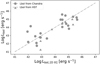 |
Fig. 1. Comparison of the bolometric values derived from the [O III] luminosities with those obtained from 2 to 10 keV Chandra and 4400 Å HST optical luminosity using X-ray and optical bolometric corrections by Duras et al. (2020). |
Main properties of the 3C subsample observed with MUSE.
These 37 radio galaxies were observed with MUSE, which is a high-throughput, wide-field of view, image-slicing integral field unit spectrograph mounted at the Very Large Telescope (VLT). Observations were performed using the Wide Field Mode sampled at 0.2 arcsec pixel−1. The observations were obtained as part of programs ID 099.B-0137(A) and 0102.B-0048(A). Each source has been observed with two exposures of 10 min, except for 3C 015 (2 × 13 min) and 3C 348 (2 × 14 min). The median seeing of the observations is 0 65. We used the ESO MUSE pipeline (version 1.6.2; Weilbacher et al. 2020) to obtain fully reduced and calibrated data cubes. The final MUSE data cube maps the entire source between 4750 Å< λ< 9300 Å. The data reduction and analysis were described in the MURALES II paper by Balmaverde et al. (2019), where all details on the data reduction are reported.
3. Searching for nuclear outflows
3.1. Data analysis
We analyzed the nuclear profile of the [O III] emission line to investigate the possible presence of nuclear outflows in the selected sample of 3C radio sources. We extracted the nuclear spectrum of each source by coadding 3 × 3 central spaxels (corresponding to 0 6 × 0
6 × 0 6) to sample a region comparable with the median seeing of the observations (0
 65).
65).
We adopted a a nonparametric approach to perform our analysis, that is, we measured the velocity percentiles, that is, velocities corresponding to a specific percentage of total flux of the [O III] emission line (e.g., Whittle 1985), thus considering the line profile as a probability distribution function. This choice was motivated by two main reasons: (i) Emission line parameters are extracted directly from the observed profile regardless of the complexity of its shape, and (ii) we can also study relatively weak [O III] emission lines for which a fitting procedure with a multicomponent model would not yield an acceptable description. To describe the kinematic of the ionized gas in the NLR, we considered these parameters:
Velocity peak (vp). The velocity corresponding to the peak of the emission line that we use as reference value for the other measurements of velocities.
Width (W80). The spectral width including 80% of the line flux, defined as the difference between the 90th and 10th percentile of the line profile (v90 and v10, respectively). For a Gaussian profile, the value W80 is close to the conventionally used full width at half maximum (Veilleux 1991).
Asymmetry (R). The asymmetry is defined by the combination of v90, v50, and v10 (the 90th, 50th, and 10th percentile of the velocity, respectively) as follows:
 (1)
(1)
It quantifies the difference of flux between the redshifted and blueshifted wing of the emission line. R shows negative values when the emission line is asymmetric toward the blueshifted side and positive values when the redshifted wing is more prominent.
Figure 2 shows how these quantities are measured in the nuclear [O III] emission line profile of 3C 033. The narrow component of the line (i.e., W80 < 600 km s−1) is usually considered a tracer of the galactic rotation and of the stellar velocity dispersion (e.g., Greene & Ho 2005; Barth et al. 2008). W80 provides information about the velocity dispersion, and R highlights the asymmetry of the emission line profile.
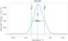 |
Fig. 2. Example of the [O III] emission-line profile (blue curve) of 3C 033 in the brightest spaxel of the image. The vertical orange line represents the velocity of the peak flux density (vp), and the green vertical lines show the 10th (v10) and 90th (v90) velocity percentiles, which are used for the definition of the velocity width of the line that contains 80% of the emission line flux (W80). In this spectrum the redshifted wing dominates, producing a positive value of the asymmetry (R > 0). The dotted red horizontal line is the continuum, linearly interpolated and subtracted. |
The fraction of the total ionized gas that moves at a higher velocity than the ordinary rotation is traced by the faint, broad wings of the [O III] line. To measure the velocity and flux of the gas in the outflow, we proceeded and adopted the following method that we illustrate in Fig. 3 for two sources, namely 3C 015 and 3C 445. First of all, we subtracted the continuum by linearly fitting two continuum bands of width 40 Å, centered at 100 Å from the line peak on the blue side (to avoid the second line of the doublet at 4959 Å) and 50 Å on the red side. Then first we estimated the centroid of the emission line as the flux-weighted wavelength vcentr in the inner region of the emission line from the peak down to one-third of the height of the peak (which we define as the core of the line). For a Gaussian profile, this value corresponds to ∼90% of the total flux of the line, and it is produced mostly by gas moving close to the systemic velocity. Second, we obtained a mirror image of the red side of the [O III] profile with respect to the vcentr axis and subtracted it from the blue side of the line. This procedure removes the symmetric component of the emission line and only leaves the asymmetric wing. Finally, we masked the core of the line, which is dominated by the gas in rotation, to obtain the component that is exclusively associated with the outflowing gas. Moreover, in the central region, the subtraction of the mirror image of the red side with the blue counterpart produces strong oscillations: the possible signatures of faint outflowing gas would be smeared out in the core of the line.
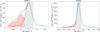 |
Fig. 3. Nuclear spectra of 3C 015 and 3C 445. Left panel: observed [O III] emission line is shown (in blue) with the mirror image of the redshifted line (in black). Their difference (in red) reveals a blueshifted wing in the profile, with ionized gas that reaches high negative velocities. We masked the central region of the [O III] profile – at one-third of the maximum height of the emission line (grey region) – not considering the gas in ordered rotation. We measured the median velocity (v50) of the outflow measured on the blue-wing residual component. |
We also defined two additional parameters for the residual wing. The median velocity of the wing (v50, wing) that corresponds to the 50th percentile of the flux contained in the wing of emission line profiles and represents the median velocity of the outflow. Positive and negative values are associated with redshifted and blueshifted wings, respectively. The flux of the wing (Fw) that is the total flux density in the wing of the emission line.
In the literature, the terminal velocity of the ionized gas is often used to explore the outflow properties. It generally corresponds to v05 or v20, that is, the flux contained in the 5th and 20th percentiles of the emission line profiles (e.g., Sturm et al. 2011; Rupke & Veilleux 2013; Veilleux et al. 2013). However, (i) these values are affected by the bulk of the emission that is dominated by rotating gas in the galaxy, therefore they may not be representative of the outflowing gas; (ii) they can only characterize the blueshifted and not the redshifted component; and (iii) they are significantly affected by the background noise because they are measured at the faint end of the profile. In Fig. 4 we compare our estimate of the outflow velocity, v50, wing, with v20. The two velocities are closely related, with a ratio of ∼1.6 (i.e., v20 ∼ 1.6 v50, wing) their level of correlation is shown in Table 2. In the following, we use v50, wing because this velocity is expected to be more representative of the velocity of the outflow and less affected by the galaxy rotational velocity field.
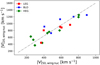 |
Fig. 4. Comparison of the velocity measured at the 20th percentile of the whole [O III] line, v20, and of the median velocity (v50, wing) of the high-velocity wing on the nucleus. The dash-dotted line corresponds to a constant ratio of 1.6. This means that in our sample, v20 would overestimate the outflow velocity. |
Statistical significance of the relations.
We estimated the uncertainties of the flux wing component Fw and v50, wing with a Monte Carlo simulation and produced mock spectra. These were obtained by varying the flux of each spectral element of the emission line profile by adding random values extracted from a normal distribution with an amplitude given by the uncertainty in each pixel. This information is stored for each pixel in the pipeline products. The uncertainties of the parameters were computed by taking the 1σ of the each parameter distribution computed from 1000 mock spectra. We consider that the outflow that is detected when the flux wing component Fw has an S/N higher than 5.
3.2. Properties of the nuclear outflows
According to the procedure and criteria described above (Sect. 3.1), we find significant nuclear outflows in about half of the sample (19 sources out of 37). Their main properties are listed in Table 3. Nuclear outflows are detected in 5 out of 6 BLOs, 9 out of 12 HEGs, and 5 out of 14 LEGs, but none in the SF galaxy. All but one source (3C 033) show blueshifted wings with v20velocities between approximately −1200 and −400 km s−1 and v50, wing velocities between −900 and −300 km s−1. In 3C 033, the high-speed residuals are located on the red side of the emission line (see Sect. 4.2 for more details).
Main properties of the nuclear outflows.
In Fig. 5 we show the median velocity of the nuclear outflow (v50, wing) as function of the AGN bolometric luminosity (Lbol) for the various spectroscopic classes of radio galaxies. To derive the bolometric luminosity from the [O III] luminosity, we adopted the correction factor proposed by Shao et al. (2013) for type 1 AGN, knowing that this average correction factor cannot be accurate for single sources. This correction is appropriate for BLOs. HEGs show the same narrow emission line ratio properties as BLOs (Buttiglione et al. 2010). However, Baldi et al. (2013) showed that their NLR is partially obscured by the circumnulear torus, causing a deficit of a factor ∼2 in line luminosity. Finally, LEGs are characterized by a different spectral energy distribution (SED) and low efficient accretion process with respect to type 1 AGNs. Nonetheless, althought the bolometric correction cannot be highly accurate for these sources, the large bolometric differences obtained between the spectroscopic classes reflect a genuinely different accretion and efficiency level. Even with this caveat, there is no clear connection between nuclear outflow velocities and bolometric luminosity or spectroscopic classes.
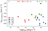 |
Fig. 5. Median velocity of the high-speed line wing (see text for details) as a function of the AGN bolometric luminosity. Green diamonds show HEGs, blue crosses show BLOs, red squares show LEGs, black circles show the spectroscopically unclassified sources, and the cyan circle represents the star forming galaxy. The empty symbols at the top of the figure represent sources without a detected line wing. The various classes show similar outflow velocities. |
The mass and energy outflow rates are important quantities for investigating the main mechanisms that drive them and their impact on the surrounding environment. First, we evaluated the fraction of the gas in outflows with respect to the total. In Fig. 6 we show the Lw, nuc/Lnuc ratio with respect to the bolometric luminosity. BLOs show typical ratio values of 0.05–0.10; the five detected outflows in the LEGs are characterized by similar fractions, and the HEGs extend to lower fractions, particularly considering the three sources without a detected nuclear outflow.
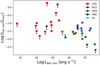 |
Fig. 6. Ratio of the [O III] luminosity of the nuclear outflowing gas with respect to the whole ionized gas in the galaxy nucleus vs. bolometric luminosity. |
We estimated the mass of the outflow using the relation discussed by Osterbrock (1989),
 (2)
(2)
ne is the electron density and LHβ is the luminosity of the Hβ emission line in erg s−1. ne is commonly measured from the emission line ratio [S II] λ6716/λ6731 (e.g., Osterbrock 1989). In principle, to estimate the electron density of the outflows, we should measure the emission line ratios only in the wings of the [S II] doublet, which is representative of the gas moving at high velocity. However, it is very challenging to deblend the [S II] doublet and take the possible presence of high-velocity wings into account, particularly in the off-nuclear regions where these lines can be very weak. In the literature we found various measurements of densities in the outflows: Nesvadba et al. (2006, 2008) derived ⟨ne⟩ = 240−570 cm−3 in two radio galaxies at z ∼ 2, Harrison et al. (2014) measured ⟨ne⟩ = 200–1000 cm−3 in a sample of low-z AGN, and Perna et al. (2015) estimated ⟨ne⟩ = 120 cm−3 in a z = 1.5 AGN. Recently, the reliability of this method for measuring ne has been questioned by Davies et al. (2020): they found that ne derived from the [S II] doublet is significantly lower than that found with ratios of auroral and transauroral lines. However, these measurements are obtained for compact radio galaxies that might be compressing gas in the very central regions of their hosts, which would produce a higher density. Following Fiore et al. (2017), we adopted an average gas density of ⟨ne⟩ = 200 cm−3 for all objects in the sample. We discuss this choice in Sect. 5. We measured the nuclear ratio [O III]/Hβ to convert the luminosity measure in the [O III] wing into the Hβ luminosity.
We then estimated the kinetic energy of nuclear outflows as
 (3)
(3)
For the undetected sources, we estimated an outflowing mass upper limit by adopting a fiducial value for the velocity of 500 km s−1. The values of the outflow mass and kinetic energy are collected in Table 4.
Energetical properties of the outflows.
The outflowing mass and kinetic energy are plotted as a function of the AGN bolometric luminosity in Fig. 7. Overall, both quantities increase with the bolometric luminosity. The median outflow mass and power in BLOs is about one order of magnitude higher than in HEGs.
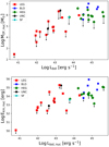 |
Fig. 7. Mass of ionized gas (top) and kinetic energy (bottom) of the nuclear outflows as a function of the AGN bolometric luminosity. The outflow mass and energy increase with the bolometric luminosity. The highest values are seen in BLOs. |
4. Searching for spatially resolved outflows
4.1. Data analysis
In addition to nuclear outflows, the MUSE data allow us to search for resolved, spatially extended outflows at kiloparsec scales. We performed the analysis described in Sect. 3 for each spaxel of the image in which the [O III] emission line is detected with an S/N > 5 in search for evidence of high-velocity asymmetric wings in the line profile. By extracting the parameters describing the line profile in each pixel, we obtained spatially resolved maps showing the 2D kinematic properties of the ionized gas. Figure 8 shows an example of the 2D property maps for the line as a whole (Fnuc, vp, W80, R) and for the high-velocity wing (Fw, v50, wing, Ekin, wing S/N) for 3C 033. The analogous diagrams for the remaining targets can be found in Appendix A.
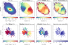 |
Fig. 8. Spatially resolved maps of the parameters defined in Sect. 4 for 3C 033. The maps are centered on the nucleus of the source, identified by the [O III] peak luminosity. Top panelfrom left to right: (1) [O III] flux, (2) velocity peak (vp) of the [O III] emission line, (3) emission line width (W80), and (4) velocity asymmetry of the [O III] profile. Bottom panelfrom left to right: (1) flux of the outflowing gas isolated by the rotational component (Fw), the black circle has a diameter of three times the seeing of the observations; (2) median velocity of the outflowing gas (v50, wing), the dashed line marks the radio position angle; (3) kinetic energy of the [O III] emitting gas; and (4) S/N of the [O III] emission residing in the line wing. In all maps, pixels with an S/N < 5 have been discarded. |
We considered an outflow to be spatially resolved if it extends to more than three times the seeing of the observations. We find 13 sources that show extended outflows. We measured the total mass and total energy carried by the outflow summing the values in all the significant pixels (i.e., with S/N > 5). We estimated the velocity of the outflow as the median value of the v50, wing and the outflow extension Rof to estimate the mass outflow rate (Ṁof) and the energy rate (Ėof); we also measured the outflow momentum boost (Ṗof). We used the continuity fluid equation for a spherical sector (see, e.g., Fiore et al. 2017),
 (4)
(4)
 (5)
(5)
 (6)
(6)
For sources without a detected extended outflow, we adopted a size limit of three times the seeing and derived the corresponding lower limits of mass and energy rates from the nuclear emission line analysis. The main properties of extended outflows that are spatially resolved are reported in Table 5, and the properties for the sources in which a lower limit has been estimated are reported in Table 4.
Properties of the extended outflows.
4.2. Properties of the extended outflows
We detected extended outflows in 13 sources: in 3 out of 6 BLOs and 10 out of 12 HEGs, in none of the 14 LEGs, and not in the SF galaxy either. The maximum spatial extent of these outflows ranges from ∼0.4 kpc (in 3C 098) to ∼20 kpc (in 3C 300), with a median value of ∼3 kpc from the nucleus. The few sources show no clear difference between the size of the outflows in HEGs and BLOs. The extended outflows show a variety of morphologies, including rather symmetric circular shapes (e.g., in 3C 227), or appear as diffuse irregular regions (e.g., in 3C 098) or filamentary emission (e.g., in 3C 079), but a bipolar structure is most commonly observed (e.g., in 3C 033, 3C 135, 3C 180, and 3C 300). Generally, HEGs show more extended structures than LEGs, consistent with the result obtained with HST (Baldi et al. 2019). A detailed description of the morphology of the extended outflows is provided in the Appendix A.
In Fig. 9 we compare the [O III] luminosity of the high-velocity wings integrated over the whole spatial extent of the outflow with that of the nuclear region. While these two estimates are similar in the three BLOs, the outflow is dominated by the extended component in the HEGs. In order to achieve a comprehensive understanding of the outflows in this sources, we must take the properties of outflowing gas derived from the line emission in these extended regions into account. For the objects without detected extended outflows, the quantities describing the “total” outflow properties are based on the nuclear measurements alone (as reported in Table 4 with the flag n).
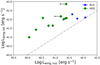 |
Fig. 9. Comparison of the [O III] luminosity of the high-velocity wing, measured in the whole outflow and in the nuclear region. The three BLOs these estimates are similar, but in the HEGs the outflow is dominated by its extended component. The dot-dashed line represents the 1:1 relation. |
The largest differences between parameters measured in the nucleus and in the total extent of the outflow are seen in the HEGs. This is likely due to the nuclear obscuration that in HEGs prevents a direct line of sight toward the nucleus of the source and at the base of the outflow, while this is visible in the BLOs. Nuclear obscuration can be the origin of the redshifted nuclear outflow found in the 3C 033. In this HEG we do not have a clear view of the central nuclear outflow, but we can observe the fast-moving ionized gas in its immediate vicinity, which shows a well-defined bipolar morphology (see Fig. 8). The redshifted component of the bipolar outflow in the central region is most likely stronger than the blueshifted component and results in a net positive outflow velocity.
In Fig. 10 (left panel) we show the total kinetic energy as a function of the bolometric luminosity: a clear linear dependence is found between these quantities. An important difference emerges compared to when nuclear regions alone are observed (Fig. 7). In the case of the nuclei, BLOs are found to be driving more powerful outflows, but when the whole outflowing region is considered, HEGs show a kinetic energy that is similar to that of BLOs. LEGs have lower bolometric luminosities than the other classes, and the detected outflows (in five sources) show correspondingly lower values of the kinetic energy. Most sources show outflow velocities between ∼200 and ∼800 km s−1, with no clear trend with Lbol or differences between the various spectroscopic classes (Fig. 10, right panel). This confirms the results from the nuclear analysis.
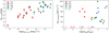 |
Fig. 10. Comparison of the outflow properties with the bolometric luminosity of the AGN (Lbol) and the Eddington ratio (Lbol/Ledd). Left panel: total kinetic energy of the outflow vs. Lbol. These quantities show a linear dependence. Right panel: velocity of the outflow vs. Lbol/Ledd. Most sources show velocities between ∼200 and ∼800 km s−1 with no clear trend with Lbol/Ledd or differences between the various spectroscopic classes. The open symbols correspond to sources without detected extended outflow. |
The momentum flow rate ṖOF can be compared to the radiation pressure force (Ṗrad = Lbol/c) to quantify the efficiency of the radiative mechanism in converting the luminosity of the AGN into the radial motion of the outflows (Zubovas & King 2012; Costa et al. 2014). In the top panel of Fig. 11, we show that the outflow momentum rate is between 10−2 and 10 of the AGN radiation pressure force, with no relation with the mean velocity. The dot-dashed line marks the expectations relative to a momentum-conserving outflow.
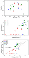 |
Fig. 11. Top panel: outflow momentum boost divided by the AGN radiation momentum rate (Lbol/c) as a function of v50, wing. The dashed line marks the expectations for a momentum conserving outflow (ṖOF/Ṗrad = 1). Middle panel: wind mass outflow rate as a function of the AGN bolometric luminosity. Bottom panel: total outflow kinetic power vs. AGN bolometric luminosity. The grey points represent the data collected by Fiore et al. (2017); the dashed line represents the relation Ėkin = 0.5% Lbol, above which an energy-driven outflow can substantially heat or blow the galactic gas out. The open symbols correspond to sources without detected extended outflow. |
Finally, in the middle and bottom panels of Fig. 11, we compare the total mass and energy rate of the outflows as a function of the bolometric luminosity. The mass outflow rate of HEGs becomes similar to that of BLOs when we consider the total outflow emission (not only the nuclear component, as in Fig. 7). The dashed line in the bottom panel represents the threshold Ėkin = 0.005 Lbol above which in an energy-driven (or energy-conserving) scenario the outflow can substantially heat or blow out the galactic gas, affecting the star formation in the host (Hopkins & Elvis 2010; Richings & Faucher-Giguere 2017). We measured a median value of Ėkin/Lbol = 0.002 in the detected sources. These low values are in line with other results in literature (e.g., Baron & Netzer 2019; Davies et al. 2020) and Fiore et al. (2017) (0.0016 measured at log Lbol = 45 erg s−1) and are consistent with values predicted by energy-driven models assuming realistic coupling efficiencies (10–20% instead of 100%, see, e.g., Costa et al. 2018; Richings & Faucher-Giguère 2018) between the accretion disk wind and the ISM.
In Fig. 11 we also compare our results with those obtained by Fiore et al. (2017), who collected observations of outflows in quasars from the literature. These authors adopted the same estimate for the gas density (200 cm−3) as we did, but a different prescription for the outflow velocity (they used the 20th velocity percentile of the [O III] emission line). Although the approach to measuring the outflow velocity is very different, as discussed in Sect. 3.1, the two measurements are closely correlated, with a median ratio of ∼1.6. This causes a systematic upward offset of 0.4 dex for the Fiore et al. estimates of Ėkin, which is much smaller than the range of measured power. We confirm that the energy rate increases with the AGN bolometric luminosity.
To explore whether there is a connection between the axis of the radio structure and of the extended outflow, we compared their orientation. An alignment between the two axes is expected considering the geometry of the central regions in which the radio jet emerges perpendicular to the plane of the accretion disk and aligned with the axis of the nuclear radiation field, consistent with what has been observed in emission-line extended morphologies of 3C radio galaxies with the HST (Baldi et al. 2019). Because several of the extended sources have circular structures with no well-defined position angle (PA), this can be successfully measured in only ten sources, see Table 1. For these sources, we show in Fig. 12 the comparison between the jet and outflow PA. The differences cover a wide range, between 0 and 60 degrees, with an only marginal preference for small offsets. This result suggests that the morphology of the outflow is mainly determined by an inhomogeneous distribution of gas in the central regions of the host galaxy and not by nuclear illumination or the jet direction. Another possibility is that jet direction and AGN illumination are not aligned. This can occur if the accretion disk (to which the jet is perpendicular) and the obscuring torus (which determines the AGN illumination cone; May et al. 2020; Goosmann & Matt 2011; Fischer et al. 2013) are not aligned.
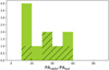 |
Fig. 12. Comparison of the position angle of the extended outflow and the radio structure. |
5. Discussion
5.1. What is the driver?
In our sample of 37 nearby radio galaxies, we have evidence of nuclear and/or extended outflows in 21 sources (57% of the sample). In radio-quiet AGN, the outflows are thought to be powered by radiation, but in radio-loud AGN the radio jet can play an important role in accelerating the wind up to kiloparsec scales (Fabian 2012). To investigate the driver of the outflows, we compared the energy (and momentum) from radiation pressure and from the radio jet to the kinetic energy (and momentum) of the outflows. We have shown that a fraction of the 0.5–10% of the bolometric luminosity is sufficient to power the observed ionized gas outflows with radiative pressure. We can now estimate the coupling efficiency required in a scenario in which the outflow is instead powered by the radio jet.
Several studies have calibrated empirical relations of the radio luminosity and the jet power, that is, the energy per unit time carried from the vicinity of the supermassive black hole to the large-scale radio source. We adopted the relation described by Daly et al. (2012)1: log Pjet = 0.84 × log P178MHz + 2.15, with both quantities in units of 1044 erg s−1.
In Fig. 13 (top panel) we compare the jet power with the bolometric luminosity estimated from the [O III] emission line. In BLOs and HEGs the bolometric luminosity is slightly higher than the jet power by a median ratio factor of 2, while in LEGs, it is lower (between 0.01 and 0.1, median ratio ∼0.07). Because we obtain values of Pjet in the same range of the Ėkin (1042–1045 erg s−1, see the bottom panel of Fig. 13), an unrealistic mechanical efficiency of η∼ 1 would be required for the radio jet to be able to accelerate the outflows in HEGs and BLOs. We cannot exclude a role of the jet in accelerating the outflow in LEGs, but this energetic argument rules out the radio jet as the main driver of the most powerful and extended outflows we observed in HEGs and BLOs. This is consistent with the fact that HEGs, LEGs, and BLOs share the same range of radio powers, but we observe more powerful and extended outflows in the most luminous sources (HEGs and BLOs) and not in the less luminous LEGs. Therefore the radiation released by the accretion process onto the SMBH seems to be the most viable mechanism to ionize and accelerate the gas to the observed velocities.
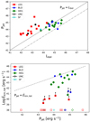 |
Fig. 13. Top panel: jet power, i.e., the energy per unit time carried from the radio jet vs. the nuclear bolometric luminosity. Bottom panel: Ėkin vs. Pjet. The dashed line represents the 1:1 relation. The jet should have an efficiency η ≈ 0.1−1 to sustain the kinetic power of the outflow. |
5.2. Energy or momentum driven?
In a momentum-driven outflow, the relativistic winds originating from the accretion disk shocks the ambient medium and cools efficiently (Ciotti & Ostriker 1997; King & Pounds 2003), transferring only its momentum flux to the ISM. Conversely, in the energy-driven or the energy-conserving outflow, the cooling of the shocked outflow from the SMBH is inefficient and generates a hot-wind bubble that expands from the center of the galaxy, transferring most of its kinetic luminosity. Hydrodynamical simulations predict that energy-driven outflows can reach momentum fluxes exceeding 10 LEdd/c within the innermost 10 kpc of the galaxy (Costa et al. 2014) and are the most massive and extended outflows.
We estimated the amount of momentum and energy transferred from the active nucleus to the ISM. These quantities assess the relative importance of AGN-driven winds in the context of galaxy evolution. One of main source of uncertainty in the measurement of the outflow energetics is the density of the outflowing gas because the ionized gas masses, and hence the kinetic energies and mass outflow rates, scale linearly with the electron density (ne). Following Fiore et al. (2017), we adopted ⟨ne⟩ = 200 cm−3 for all objects in the sample. Our estimates might need to be rescaled for different values of the density, but the relative comparison between different sources is robust because we do not expect large variation in the gas density of the outflows from source to source.
We obtained mass outflow rates in the range of 0.4−30 M⊙ yr−1 and kinetic energies of about 1042–1045 erg−1 and ṖOF/Ṗrad between ∼0.01 and 10, with observed v20 velocities in the range 400–1500 km s−1. These values are similar to what is observed in other types of AGNs within the rather large uncertainties. For example, Harrison et al. (2014) analyzed IFU observations of 16 type 2 AGN below redshift 0.2 with a similar bolometric luminosity range (∼1044–1046 erg s−1), and found high velocities in the range 510–1100 km s−1 in all their targets. In 70% of the sample, the outflow is resolved and extended on kiloparsec scales. They estimated an energy outflow rate of about (0.15−45) × 1044 erg s−1, which matches our results. Fiore et al. (2017) found that about half of the ionized winds have ṖOF/Ṗrad ≲ 1, and the other half has ≳1 and a few > 10, suggesting that these latter ionized winds may also be energy conserving. Energy-conserving winds are characterized by values of ṖOF/Ṗrad of 15–20 (e.g., Faucher-Giguère & Quataert 2012; Zubovas & King 2012). Conversely, values of ṖOF/Ṗrad ≲ 10 suggest that these ionized winds are momentum conserving, as predicted by the King & Pounds (2003) model. The low outflow momentum boost we obtained (see Fig. 11, top panel) suggests a momentum-conserving (radiative) regime, as observed in BAL winds and fast X-ray winds. However, we recall that the contribution of molecular and neutral atomic phase might be significant and increase the momentum boost: the ionized gas is usually the less important part in terms of mass and energies when multiphase outflow studies are available (see, e.g., Carniani et al. 2017; Fiore et al. 2017; Fluetsch et al. 2019).
5.3. Connection between outflow and nuclear properties
The existence of a link between the bolometric luminosity of the AGN and the velocity of the outflow is controversial. There are claims for a positive correlation (e.g., Mullaney et al. 2013), but other authors using different samples find, in agreement with our results for the 3C radio galaxies, no clear trend between these quantities (Harrison et al. 2014). Using a different sample of objects, Bischetti et al. (2017) reported a correlation between the maximum outflow velocity and AGN luminosity that is absent when the individual samples are considered separately. We note that this trend is expected for energy-conserving winds ( , Costa et al. 2014) and may explain why we do not see this relation in our sample, in which the data suggest that the outflows are produced by momentum-conserving winds.
Instead, we find a positive trend between the kinetic energy of the outflow and the bolometric luminosity. Standard measurements of the outflow velocity based on percentile velocities of the whole line, that is, v20, might be subject to a bias because stronger emission lines have more luminous wings, inducing the observed correlation. However, our approach for measuring the outflow velocity accounts for this bias, and we argue that this positive trend is a robust result.
5.4. Differences between LEGs, HEGs and BLOs
The clearest differences between different spectroscopic types is that all LEGs appear to be compact (we estimated an average upper limit of 1 kpc) and only HEGs and BLOs show extended outflows. The average radius is 4 kpc for HEGs and 3 kpc for BLOs. Moreover, LEGs accelerate a larger fraction of the gas: about 10% of the total ionized gas is part of the outflow, compared to ∼1% in HEGs and BLOs. The outflow velocities are comparable, but in LEGs, we detect lower mass rate and kinetic energy in the outflows.
The observed differences of the outflow in HEG and LEGs might be due to different environments (e.g., Macconi et al. 2020). LEGs are more frequently found in clusters than BLOs or HEGs (Ramos Almeida et al. 2013), and their supermassive black holes are thought to accrete mainly hot gas. Many radio galaxies of LEG type are able to displace the hot, X-ray emitting gas with radio jets and lobes. HEGs are thought to have larger amounts of cold gas, supported by the presence of a dusty torus and efficient accretion. In theoretical models, it is relatively easy to displace the hot, diffuse interstellar medium, but it is more difficult to hydrodynamically accelerate cold clouds. Recent simulations have shown that a combination of instabilities and simple pressure gradients will drive the cloud material to effectively expand in the direction perpendicular to the incident outflow. In this case, the outflow can effectively expand in the direction perpendicular to the incident outflow and propagate out to large radii. We speculate that the large extent of the ionized outflows present in HEGs and BLOs might be related to the large amount of cold gas with respect to LEGs and to a more powerful ionizing nucleus.
5.5. Effect of outflows
To evaluate whether the ionized outflowing gas can permanently escape the galaxy, we estimate the escape velocity vesc from the host. We used the prescription by Desai et al. (2004), which links the circular velocities vc to the line-of-sight stellar velocity dispersion σ (vc ≈ 1.54σ) and the relation by Rupke et al. (2002), who adopted a simple gravitational model based on an isothermal sphere, which predicts ![Mathematical equation: $ v_{\mathrm{esc}}(r) = \sqrt2 v_{\mathrm{c}}[1+\ln (r_{\max}/r)]^{(1/2)} $](/articles/aa/full_html/2021/09/aa40686-21/aa40686-21-eq12.gif) . For a galaxy with a velocity dispersion of 300 km s−1 at a radius of r = 10 kpc and assuming rmax = 100 kpc, we estimate a typical escape velocity of ∼1170 km s−1. We measured outflow velocities well below this threshold and outflowing gas masses of about a few solar masses per year.
. For a galaxy with a velocity dispersion of 300 km s−1 at a radius of r = 10 kpc and assuming rmax = 100 kpc, we estimate a typical escape velocity of ∼1170 km s−1. We measured outflow velocities well below this threshold and outflowing gas masses of about a few solar masses per year.
We infer that the outflowing gas cannot leave the gravitational potential well of the host galaxy, even if the radio jet facilitates pushing this gas out (Fromm et al. 2018; Best et al. 2005). This result, combined with the relatively low values of conversion between bolometric luminosity and outflow energy rate, Ėkin/Lbol = 0.2%, suggests that the observed outflows are not able to significantly affect the gas content or the star formation in the host. This could be consistent with an auto-regulating feedback-feeding mechanism proposed by Gaspari et al. (2020), for example.
6. Summary and conclusions
We have observed 37 3C radio galaxies at z < 0.3 with the VLT/MUSE integral field spectrograph, obtained in the framework of the MURALES project. The main aim of this paper was to explore ionized outflows and the relation with the radio jet. This sample includes all spectroscopic subtypes of radio galaxies, LEGs, HEGs, and BLOs.
We performed a nonparametric analysis of the [O III] emission line, exploring the asymmetries in the wings of the line profile. We measured v50, wing, the mean velocity of the wings residuals. We consider this definition more representative of the outflow velocity than the percentile velocities that are commonly used in literature, which are typically affected by the entire flux emission, that is, are dominated by gravitational motions. However, for a comparison with other studies in literature, we also measured v20 and found a good correlation with v50, wing, with v20 larger than v50, wing by a median factor 1.6.
We found evidence of nuclear outflows in 21 sources (5 out of 6 BLOs, 9 out of 12 HEGs, and 5 out of 14 LEGs) with blueshifted v20 velocities between ∼1200 and ∼400 km s−1 and v50, wing velocities between ∼300 and ∼900 km s−1 (still blueshifted). We observed only one redshifted wing in 3C 033, likely because of obscuration in the nuclear region. We measured the luminosity of the wing and the kinetic energy of the outflow.
The same analysis, performed in all spaxels, revealed extended outflows in 13 sources with sizes between 0.4 and 20 kpc. Comparing the luminosity and kinetic energy of these extended outflows with those obtained from the nuclear analysis, we found large differences between parameters measured on the nucleus and on the total extent of the outflow in HEGs, likely due to a combination of prominent extended outflows and nuclear obscuration. To provide a more comprehensive view of the outflows in these sources, we therefore included measurements of these extended regions. For the objects without detected extended outflows, the quantities describing the total outflow properties are based on the nuclear measurements alone. We measured the mass and kinetic energy outflow rates assuming an outflow radius corresponding to the maximum observed extension of the outflows (for the compact sources, we assumed a radius equal to three times the seeing of the observations, and we provided lower limits) and as velocity the mean value of v50, wing in the outflow region.
We detected nuclear and/or extended outflows in 21 out of 37 radio sources we analyzed. We observed different outflow morphologies, but they were mainly circular or bipolar. In the extended outflows where we are able to estimate the orientation, this is not closely correlated with the radio jet direction. This is likely due to an inhomogeneous distribution of the gas in the host galaxy possibly produced by the jet expansion that drives away gas along its path. We found mass outflow rates and kinetic energy rates in line with the values obtained by studying other samples of quasars (Mof ∼ 0.4−30 M⊙ yr−1, Ėkin ∼ 1042 − 1045 erg s−1), but with a low momentum loading factor ṖOF/Ṗrad < 10. This result suggests that our outflows probably are momentum driven and not energy driven, as observed in many X-ray fast winds and BALs and also in many galactic-scale ionized outflows; see, for example, the right panel of Fig. 2 in Fiore et al. (2017).
Comparing the nuclear bolometric luminosity and the jet power, we speculate that these winds are likely accelerated by the radiation released by the accretion process and not by the radio jet, at least in HEGs and BLOs. In these sources, the radio power is even a factor 10 lower than the bolometric luminosity, and a mechanical efficiency of about 1 would be required by the radio jet to accelerate the outflows. In LEGs, the bolometric luminosity is lower than the jet power, and we cannot exclude a strong contribution of the jet to the acceleration process.
We conclude that nuclear outflows are common in radio galaxies, and that they are extended in almost all the HEGs and BLOs, in which the nuclear radiation powers the outflow. The velocities, gas mass, and kinetic energy rate are probably too low to have a significant effect on the host galaxy. However, the ionized gas is just one of the outflow phases, which also include atomic and molecular gas. In order to obtain a full characterization of the properties and effect of the AGN outflows in the population of radio galaxies, multiphase observations of our sample are required.
This relation has been calibrated considering a sample of FRII radio galaxies, but it agrees with the relations from Willott et al. (1999) and Cavagnolo et al. (2010), who considered sample of FRI radio galaxies.
Acknowledgments
We acknowledge the anonymous referee for her/his report. Based on observations collected at the European Organisation for Astronomical Research in the Southern Hemisphere under ESO programmes 0102.B-0048(A) 099.B-0137(A). This research has made use of the NASA/IPAC Extragalactic Database (NED), which is operated by the Jet Propulsion Laboratory, California Institute of Technology, under contract with the National Aeronautics and Space Administration. This work is supported by the “Departments of Excellence 2018–2022” Grant awarded by the Italian Ministry of Education, University and Research (MIUR) (L. 232/2016). This investigation is supported by the National Aeronautics and Space Administration (NASA) grants GO9-20083X and GO0-21110X. GS acknowledges financial support from the European Union’s Horizon 2020 research and innovation programme under Marie Skłodowska-Curie grant agreement No. 860744 (BID4BEST), from the State Research Agency (AEI-MCINN) of the Spanish MCIU under grant “Feeding and feedback in active galaxies” with reference PID2019-106027GB-C42, and from IAC project P/301404, financed by the Ministry of Science and Innovation, through the State Budget and by the Canary Islands Department of Economy, Knowledge and Employment, through the Regional Budget of the Autonomous Community. GV acknowledges support from ANID program FONDECYT Postdoctorado 3200802. SB and CO acknowledge support from the Natural Sciences and Engineering Research Council (NSERC) of Canada. BAT was supported by the Harvard Future Faculty Leaders Postdoctoral Fellowship.
References
- Aditya, J. N. H. S., & Kanekar, N. 2018, MNRAS, 473, 59 [NASA ADS] [CrossRef] [Google Scholar]
- Aird, J., Coil, A. L., Georgakakis, A., et al. 2015, MNRAS, 451, 1892 [NASA ADS] [CrossRef] [Google Scholar]
- Axon, D. J., Marconi, A., Capetti, A., et al. 1998, ApJ, 496, L75 [NASA ADS] [CrossRef] [Google Scholar]
- Baldi, R. D., & Capetti, A. 2008, A&A, 489, 989 [NASA ADS] [CrossRef] [EDP Sciences] [Google Scholar]
- Baldi, R. D., & Capetti, A. 2010, A&A, 519, A48 [NASA ADS] [CrossRef] [EDP Sciences] [Google Scholar]
- Baldi, R. D., Capetti, A., Buttiglione, S., Chiaberge, M., & Celotti, A. 2013, A&A, 560, A81 [NASA ADS] [CrossRef] [EDP Sciences] [Google Scholar]
- Baldi, R. D., Rodríguez Zaurín, J., Chiaberge, M., et al. 2019, ApJ, 870, 53 [NASA ADS] [CrossRef] [Google Scholar]
- Balmaverde, B., Baldi, R. D., & Capetti, A. 2008, A&A, 486, 119 [NASA ADS] [CrossRef] [EDP Sciences] [Google Scholar]
- Balmaverde, B., Capetti, A., Marconi, A., & Venturi, G. 2018a, A&A, 612, A19 [NASA ADS] [CrossRef] [EDP Sciences] [Google Scholar]
- Balmaverde, B., Capetti, A., Marconi, A., et al. 2018b, A&A, 619, A83 [NASA ADS] [CrossRef] [EDP Sciences] [Google Scholar]
- Balmaverde, B., Capetti, A., Marconi, A., et al. 2019, A&A, 632, A124 [CrossRef] [EDP Sciences] [Google Scholar]
- Baron, D., & Netzer, H. 2019, MNRAS, 486, 4290 [NASA ADS] [CrossRef] [Google Scholar]
- Barth, A. J., Greene, J. E., & Ho, L. C. 2008, AJ, 136, 1179 [NASA ADS] [CrossRef] [Google Scholar]
- Baum, S. A., Gallimore, J. F., O’Dea, C. P., et al. 2010, ApJ, 710, 289 [NASA ADS] [CrossRef] [Google Scholar]
- Bennett, C. L., Larson, D., Weiland, J. L., & Hinshaw, G. 2014, ApJ, 794, 135 [NASA ADS] [CrossRef] [Google Scholar]
- Best, P. N., & Heckman, T. M. 2012, MNRAS, 421, 1569 [NASA ADS] [CrossRef] [Google Scholar]
- Best, P. N., Kauffmann, G., Heckman, T. M., et al. 2005, MNRAS, 362, 25 [NASA ADS] [CrossRef] [Google Scholar]
- Bîrzan, L., Rafferty, D. A., McNamara, B. R., Wise, M. W., & Nulsen, P. E. J. 2004, ApJ, 607, 800 [NASA ADS] [CrossRef] [Google Scholar]
- Bîrzan, L., Rafferty, D. A., Nulsen, P. E. J., et al. 2012, MNRAS, 427, 3468 [NASA ADS] [CrossRef] [Google Scholar]
- Bischetti, M., Piconcelli, E., Vietri, G., et al. 2017, A&A, 598, A122 [NASA ADS] [CrossRef] [EDP Sciences] [Google Scholar]
- Brusa, M., Bongiorno, A., Cresci, G., et al. 2015, MNRAS, 446, 2394 [NASA ADS] [CrossRef] [Google Scholar]
- Buttiglione, S., Capetti, A., Celotti, A., et al. 2009, A&A, 495, 1033 [NASA ADS] [CrossRef] [EDP Sciences] [Google Scholar]
- Buttiglione, S., Capetti, A., Celotti, A., et al. 2010, A&A, 509, A6 [NASA ADS] [CrossRef] [EDP Sciences] [Google Scholar]
- Buttiglione, S., Capetti, A., Celotti, A., et al. 2011, A&A, 525, A28 [NASA ADS] [CrossRef] [EDP Sciences] [Google Scholar]
- Capetti, A., Axon, D. J., Macchetto, F. D., Marconi, A., & Winge, C. 1999, ApJ, 516, 187 [NASA ADS] [CrossRef] [Google Scholar]
- Cardelli, J. A., Clayton, G. C., & Mathis, J. S. 1989, ApJ, 345, 245 [NASA ADS] [CrossRef] [Google Scholar]
- Carniani, S., Marconi, A., Maiolino, R., et al. 2017, A&A, 605, A105 [NASA ADS] [CrossRef] [EDP Sciences] [Google Scholar]
- Cavagnolo, K. W., McNamara, B. R., Nulsen, P. E. J., et al. 2010, ApJ, 720, 1066 [NASA ADS] [CrossRef] [Google Scholar]
- Chiaberge, M., Capetti, A., & Celotti, A. 2000, A&A, 355, 873 [NASA ADS] [Google Scholar]
- Chiaberge, M., Macchetto, F. D., Sparks, W. B., et al. 2002, ApJ, 571, 247 [NASA ADS] [CrossRef] [Google Scholar]
- Cicone, C., Feruglio, C., Maiolino, R., et al. 2012, A&A, 543, A99 [NASA ADS] [CrossRef] [EDP Sciences] [Google Scholar]
- Ciotti, L., & Ostriker, J. P. 1997, ApJ, 487, L105 [NASA ADS] [CrossRef] [Google Scholar]
- Costa, T., Sijacki, D., & Haehnelt, M. G. 2014, MNRAS, 444, 2355 [Google Scholar]
- Costa, T., Rosdahl, J., Sijacki, D., & Haehnelt, M. G. 2018, MNRAS, 473, 4197 [NASA ADS] [CrossRef] [Google Scholar]
- Couto, G. S., Storchi-Bergmann, T., & Schnorr-Müller, A. 2017, MNRAS, 469, 1573 [NASA ADS] [CrossRef] [Google Scholar]
- Couto, G. S., Storchi-Bergmann, T., Siemiginowska, A., Riffel, R. A., & Morganti, R. 2020, MNRAS, 497, 5103 [NASA ADS] [CrossRef] [Google Scholar]
- Crenshaw, D. M., Schmitt, H. R., Kraemer, S. B., Mushotzky, R. F., & Dunn, J. P. 2010, ApJ, 708, 419 [Google Scholar]
- Crenshaw, D. M., Fischer, T. C., Kraemer, S. B., & Schmitt, H. R. 2015, ApJ, 799, 83 [NASA ADS] [CrossRef] [Google Scholar]
- Daly, R. A., Sprinkle, T. B., O’Dea, C. P., Kharb, P., & Baum, S. A. 2012, MNRAS, 423, 2498 [NASA ADS] [CrossRef] [Google Scholar]
- Davies, R., Baron, D., Shimizu, T., et al. 2020, MNRAS, 498, 4150 [Google Scholar]
- Desai, V., Dalcanton, J. J., Mayer, L., et al. 2004, MNRAS, 351, 265 [NASA ADS] [CrossRef] [Google Scholar]
- Duras, F., Bongiorno, A., Ricci, F., et al. 2020, A&A, 636, A73 [CrossRef] [EDP Sciences] [Google Scholar]
- Dutton, A. A., & van den Bosch, F. C. 2009, MNRAS, 396, 141 [NASA ADS] [CrossRef] [Google Scholar]
- Fabian, A. C. 2012, ARA&A, 50, 455 [Google Scholar]
- Faucher-Giguère, C.-A., & Quataert, E. 2012, MNRAS, 425, 605 [NASA ADS] [CrossRef] [Google Scholar]
- Ferrarese, L., & Merritt, D. 2000, ApJ, 539, L9 [Google Scholar]
- Fiore, F., Feruglio, C., Shankar, F., et al. 2017, A&A, 601, A143 [NASA ADS] [CrossRef] [EDP Sciences] [Google Scholar]
- Fischer, T. C., Crenshaw, D. M., Kraemer, S. B., & Schmitt, H. R. 2013, ApJS, 209, 1 [NASA ADS] [CrossRef] [Google Scholar]
- Fluetsch, A., Maiolino, R., Carniani, S., et al. 2019, MNRAS, 483, 4586 [NASA ADS] [Google Scholar]
- Fromm, C. M., Perucho, M., Porth, O., et al. 2018, A&A, 609, A80 [NASA ADS] [CrossRef] [EDP Sciences] [Google Scholar]
- Gaspari, M., Tombesi, F., & Cappi, M. 2020, Nat. Astron., 4, 10 [Google Scholar]
- Gebhardt, K., Bender, R., Bower, G., et al. 2000, ApJ, 539, L13 [Google Scholar]
- Goosmann, R. W., & Matt, G. 2011, MNRAS, 415, 3119 [NASA ADS] [CrossRef] [Google Scholar]
- Greene, J. E., & Ho, L. C. 2005, ApJ, 627, 721 [NASA ADS] [CrossRef] [Google Scholar]
- Haas, M., Siebenmorgen, R., Schulz, B., Krügel, E., & Chini, R. 2005, A&A, 442, L39 [NASA ADS] [CrossRef] [EDP Sciences] [Google Scholar]
- Hardcastle, M. J., Evans, D. A., & Croston, J. H. 2006, MNRAS, 370, 1893 [NASA ADS] [CrossRef] [Google Scholar]
- Hardcastle, M. J., Evans, D. A., & Croston, J. H. 2009, MNRAS, 396, 1929 [NASA ADS] [CrossRef] [Google Scholar]
- Hardcastle, M. J., Ching, J. H. Y., Virdee, J. S., et al. 2013, MNRAS, 429, 2407 [NASA ADS] [CrossRef] [Google Scholar]
- Harrison, C. M., Alexander, D. M., Mullaney, J. R., & Swinbank, A. M. 2014, MNRAS, 441, 3306 [Google Scholar]
- Hopkins, P. F., & Elvis, M. 2010, MNRAS, 401, 7 [NASA ADS] [CrossRef] [Google Scholar]
- Jimenez-Gallardo, A., Massaro, F., Prieto, M. A., et al. 2020, ApJS, 250, 7 [Google Scholar]
- King, A. R., & Pounds, K. A. 2003, MNRAS, 345, 657 [NASA ADS] [CrossRef] [Google Scholar]
- King, A., & Pounds, K. 2015, ARA&A, 53, 115 [NASA ADS] [CrossRef] [Google Scholar]
- Kormendy, J., & Ho, L. C. 2013, ARA&A, 51, 511 [Google Scholar]
- Koski, A. T. 1978, ApJ, 223, 56 [NASA ADS] [CrossRef] [Google Scholar]
- Laing, R. A., Jenkins, C. R., Wall, J. V., & Unger, S. W. 1994, in The Physics of Active Galaxies, eds. G. V. Bicknell, M. A. Dopita, & P. J. Quinn, ASP Conf. Ser., 54, 201 [Google Scholar]
- Macconi, D., Torresi, E., Grandi, P., Boccardi, B., & Vignali, C. 2020, MNRAS, 493, 4355 [CrossRef] [Google Scholar]
- Mahony, E. K., Oonk, J. B. R., Morganti, R., et al. 2016, MNRAS, 455, 2453 [NASA ADS] [CrossRef] [Google Scholar]
- Massaro, F., Harris, D. E., Tremblay, G. R., et al. 2010, ApJ, 714, 589 [NASA ADS] [CrossRef] [Google Scholar]
- Massaro, F., Tremblay, G. R., Harris, D. E., et al. 2012, ApJS, 203, 31 [NASA ADS] [CrossRef] [Google Scholar]
- Massaro, F., Harris, D. E., Liuzzo, E., et al. 2015, ApJS, 220, 5 [NASA ADS] [CrossRef] [Google Scholar]
- Massaro, F., Missaglia, V., Stuardi, C., et al. 2018, ApJS, 234, 7 [NASA ADS] [CrossRef] [Google Scholar]
- May, D., Steiner, J. E., Menezes, R. B., Williams, D. R. A., & Wang, J. 2020, MNRAS, 496, 1488 [NASA ADS] [CrossRef] [Google Scholar]
- McNamara, B. R., & Nulsen, P. E. J. 2012, New J. Phys., 14 [Google Scholar]
- McNamara, B. R., Wise, M., Nulsen, P. E. J., et al. 2000, ApJ, 534, L135 [CrossRef] [Google Scholar]
- Mingozzi, M., Cresci, G., Venturi, G., et al. 2019, A&A, 622, A146 [NASA ADS] [CrossRef] [EDP Sciences] [Google Scholar]
- Morganti, R. 2019, Proc. IAU, 15, 229 [NASA ADS] [CrossRef] [Google Scholar]
- Morganti, R., & Oosterloo, T. 2018, A&ARv, 26, 4 [NASA ADS] [CrossRef] [Google Scholar]
- Morganti, R., Oosterloo, T. A., Emonts, B. H. C., van der Hulst, J. M., & Tadhunter, C. N. 2003, ApJ, 593, L69 [NASA ADS] [CrossRef] [Google Scholar]
- Morganti, R., Tadhunter, C. N., & Oosterloo, T. A. 2005, A&A, 444, L9 [NASA ADS] [CrossRef] [EDP Sciences] [Google Scholar]
- Mukherjee, D., Bicknell, G. V., Sutherland, R., & Wagner, A. 2016, MNRAS, 461, 967 [NASA ADS] [CrossRef] [Google Scholar]
- Mullaney, J. R., Alexander, D. M., Fine, S., et al. 2013, MNRAS, 433, 622 [NASA ADS] [CrossRef] [Google Scholar]
- Nesvadba, N. P. H., Lehnert, M. D., Eisenhauer, F., et al. 2006, ApJ, 650, 693 [NASA ADS] [CrossRef] [Google Scholar]
- Nesvadba, N. P. H., Lehnert, M. D., De Breuck, C., Gilbert, A. M., & van Breugel, W. 2008, A&A, 491, 407 [NASA ADS] [CrossRef] [EDP Sciences] [Google Scholar]
- Oppenheimer, B. D., & Davé, R. 2006, MNRAS, 373, 1265 [NASA ADS] [CrossRef] [Google Scholar]
- Osterbrock, D. E. 1977, ApJ, 215, 733 [Google Scholar]
- Osterbrock, D. E. 1989, J. R. Astron. Soc. Can., 83, 345 [NASA ADS] [Google Scholar]
- Perna, M., Brusa, M., Cresci, G., et al. 2015, A&A, 574, A82 [NASA ADS] [CrossRef] [EDP Sciences] [Google Scholar]
- Ramos Almeida, C., Bessiere, P. S., Tadhunter, C. N., et al. 2013, MNRAS, 436, 997 [NASA ADS] [CrossRef] [Google Scholar]
- Revalski, M., Crenshaw, D. M., Kraemer, S. B., et al. 2018, ApJ, 856, 46 [NASA ADS] [CrossRef] [Google Scholar]
- Richings, A. J., & Faucher-Giguere, C.-A. 2017, The Galaxy Ecosystem: Flow of Baryons through Galaxies (Garching), 3 [Google Scholar]
- Richings, A. J., & Faucher-Giguère, C.-A. 2018, MNRAS, 478, 3100 [NASA ADS] [CrossRef] [Google Scholar]
- Rochais, T. B., DiPompeo, M. A., Myers, A. D., et al. 2014, MNRAS, 444, 2498 [NASA ADS] [CrossRef] [Google Scholar]
- Rupke, D. S. N., & Veilleux, S. 2013, ApJ, 775, L15 [NASA ADS] [CrossRef] [Google Scholar]
- Rupke, D. S., Veilleux, S., & Sanders, D. B. 2002, ApJ, 570, 588 [NASA ADS] [CrossRef] [Google Scholar]
- Santoro, F., Tadhunter, C., Baron, D., Morganti, R., & Holt, J. 2020, A&A, 644, A54 [NASA ADS] [CrossRef] [EDP Sciences] [Google Scholar]
- Schawinski, K., Urry, C. M., Simmons, B. D., et al. 2014, MNRAS, 440, 889 [Google Scholar]
- Shao, L., Kauffmann, G., Li, C., Wang, J., & Heckman, T. M. 2013, MNRAS, 436, 3451 [CrossRef] [Google Scholar]
- Silk, J., & Rees, M. J. 1998, A&A, 331, L1 [NASA ADS] [Google Scholar]
- Spoon, H. W. W., & Holt, J. 2009, ApJ, 702, L42 [NASA ADS] [CrossRef] [Google Scholar]
- Stuardi, C., Missaglia, V., Massaro, F., et al. 2018, ApJS, 235, 32 [Google Scholar]
- Sturm, E., González-Alfonso, E., Veilleux, S., et al. 2011, ApJ, 733, L16 [NASA ADS] [CrossRef] [Google Scholar]
- Tadhunter, C. N., Villar-Martin, M., Morganti, R., Bland-Hawthorn, J., & Axon, D. 2000, MNRAS, 314, 849 [NASA ADS] [CrossRef] [Google Scholar]
- Tombesi, F., Tazaki, F., Mushotzky, R. F., et al. 2014, MNRAS, 443, 2154 [NASA ADS] [CrossRef] [Google Scholar]
- Veilleux, S. 1991, ApJ, 369, 331 [Google Scholar]
- Veilleux, S., Meléndez, M., Sturm, E., et al. 2013, ApJ, 776, 27 [NASA ADS] [CrossRef] [Google Scholar]
- Venturi, G., Nardini, E., Marconi, A., et al. 2018, A&A, 619, A74 [NASA ADS] [CrossRef] [EDP Sciences] [Google Scholar]
- Wagner, A. Y., Bicknell, G. V., & Umemura, M. 2012, ApJ, 757, 136 [NASA ADS] [CrossRef] [Google Scholar]
- Weilbacher, P. M., Palsa, R., Streicher, O., et al. 2020, A&A, 641, A28 [CrossRef] [EDP Sciences] [Google Scholar]
- Weymann, R. J., Morris, S. L., Foltz, C. B., & Hewett, P. C. 1991, ApJ, 373, 23 [NASA ADS] [CrossRef] [Google Scholar]
- Whittle, M. 1985, MNRAS, 213, 1 [NASA ADS] [CrossRef] [Google Scholar]
- Willott, C. J., Rawlings, S., Blundell, K. M., & Lacy, M. 1999, MNRAS, 309, 1017 [Google Scholar]
- Zakamska, N. L., & Greene, J. E. 2014, MNRAS, 442, 784 [Google Scholar]
- Zubovas, K., & King, A. 2012, ApJ, 745, L34 [Google Scholar]
Appendix A: Nuclear spectra and spatially resolved maps of kinematical parameters
In Fig. A.1 we present for all objects analogs of Fig. 3, that is, the nuclear spectrum extracted from the central 0 6 × 0
6 × 0 6, showing the decomposition of the [O III] profile into rotating and outflowing gas. In six sources (3C 089, 3C 318.1, 3C 386, and 3C 403.1), the [O III] emission line is not detected, and they were not considered for this analysis.
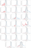 |
Fig. A.1. Nuclear spectra of the 33 3C sources with a detection of the [O III] emission line. Superposed on the [O III] profile (blue) is the mirror image of the redshifted line (black). Their difference (red) reveals any line asymmetry. We estimated the median velocity (V50) of the asymmetric line wing and its flux (Fw), after masking the spectral region at one-third of the maximum height of the profile (grey region). |
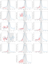 |
Fig. A.1. continued. |
Finally, in Figs. A.2 through A.26 we show the maps of the eight parameters defined in Sect. 4, that is, the velocity peak (vp) of the [O III] emission-line, the emission line width (W80), the line asymmetry, the S/N peak of the whole [O III] line, the flux of the outflowing gas isolated by the rotational component (Fw), the median velocity of the outflowing gas (v50, wing), the kinetic energy of the [O III] emitting gas, and the S/N of the [O III] emission residing in the line wing. The last four parameters are estimated only in pixels with an S/N > 5. In the panel showing the line wing flux, we draw a circle with a diameter of three times the seeing of the observations: the sources in which the wing is observed at larger distances are considered as those associated with an extended outflow. In the panel showing the wing velocity, the dashed line marks the radio position angle.
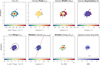 |
Fig. A.2. 3C 015, LEG, 1″ = 1.36 kpc. The black circle in the first panel has a diameter of 3 times the seeing of the observations; the dashed line in the second panel marks the radio position angle. Its nuclear outflow appear to be confined in a circular region of radius ∼0.98 kpc and having a blue-shifted component peaking at ∼ − 890 km s−1. The outflow is well resolved enabling us to observe a kinetic energy increasing towards the center. |
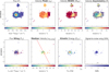 |
Fig. A.3. 3C 017, BLO, 1″ = 3.37 kpc. The black circle in the first panel has a diameter of 3 times the seeing of the observations; the dashed line in the second panel marks the radio position angle. The outflowing gas is moving toward us reaching negative values of velocity. Unfortunately its compactness (the upper limit of its extension from the center is ∼1.68 kpc) prevent us from producing a well resolved map of its kinetic energy. The ionized gas achieves a velocity up to ∼ − 1100 km s−1. |
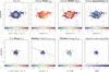 |
Fig. A.4. 3C 018, BLO, 1″ = 3.00 kpc. The black circle in the first panel has a diameter of 3 times the seeing of the observations; the dashed line in the second panel marks the radio position angle. The ionized gas appears well resolved, reaching high negative velocities up to ∼ − 1120 km s−1. The kinetic energy gradually decrease from the central nucleus to the edge (∼2.52 kpc). |
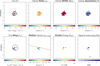 |
Fig. A.5. 3C 029, LEG, 1″ = 0.88 kpc. The black circle in the first panel has a diameter of 3 times the seeing of the observations; the dashed line in the second panel marks the radio position angle. Similarly to 3C 017 the emission line are only few extended and not well resolved. The maximum extension is reached in the SW region at ∼0.20 kpc from the nucleus. We observe only the blue component of the outflow. |
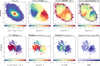 |
Fig. A.6. 3C 033, HEG, 1″ = 1.14 kpc. The black circle in the first panel has a diameter of 3 times the seeing of the observations; the dashed line in the second panel marks the radio position angle. We observe an outflow symmetrically extended towards the NW and the SE directions out to ∼3.4″ (∼3.88 kpc) from the nucleus. In the NW region the gas assumes positive velocities (up to ∼1800 km s−1) and in the SE negative values (up to ∼2000 km s−1), in both cases they slowly decrease along the maximum extension. The kinetic energy grows from the most external regions close to the center, reaching the maximum values at ∼1.00 kpc from the nucleus and decreasing again approaching the center. This is due to our field of view in which the nucleus is obscured by the torus surrounding the central engine. In fact the highest values of S/N are measured in the same area in which the energy gets the greatest values. |
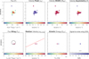 |
Fig. A.7. 3C 040, LEG, 1″ = 0.36 kpc. The black circle in the first panel has a diameter of 3 times the seeing of the observations; the dashed line in the second panel marks the radio position angle. |
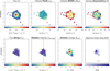 |
Fig. A.8. 3C 063, HEG, 1″ = 1.36 kpc. The black circle in the first panel has a diameter of 3 times the seeing of the observations; the dashed line in the second panel marks the radio position angle. The gas in outflow shows a quite circular shape with a radius of ∼1.14 kpc with a elongation in the SE direction (∼ out to 2.12 kpc). We observe just the blue component of the [O III] with a velocity down to ∼1900 km s−1. |
 |
Fig. A.9. 3C 079, HEG, 1″ = 3.75 kpc. The black circle in the first panel has a diameter of 3 times the seeing of the observations; the dashed line in the second panel marks the radio position angle. The outflow gas is confined in a circular region of radius ∼7.5 kpc, from here two filamentary structures extend beyond ∼36 kpc and ∼26 kpc respectively towards NE and SW. The filaments appears as the division axis between the gas launched in our direction (upper area) and the one in the opposite side (bottom area). The central region of the source is obscured, prevent us to observe the energetic of the nucleus. The maximum velocity achieved by the [O III] is ∼2450 km s−1, that represents the maximum velocity reached by the outflow in the whole sample and also by the 3C 180. |
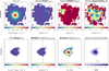 |
Fig. A.10. 3C 088, LEG, 1″ = 0.60 kpc. The black circle in the first panel has a diameter of 3 times the seeing of the observations; the dashed line in the second panel marks the radio position angle. The source is well resolved, the kinetic energy of the gas increases in the inner part and its velocities are negative out to ∼ − 1360 km s−1. The outflow not expands beyond 0.72 kpc from the nucleus. |
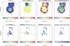 |
Fig. A.11. 3C 098, LEG, 1″ = 0.60 kpc. The black circle in the first panel has a diameter of 3 times the seeing of the observations; the dashed line in the second panel marks the radio position angle. The MUSE field-of-view covers only ∼1/4 of the extension of the radio source. Even if the map is not well resolved we can see that the ionized gas of the outflow reaching negative velocities beyond ∼2000 km s−1 and it expands into an irregular structure. |
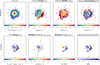 |
Fig. A.12. 3C 105, BLO, 1″ = 1.63 kpc. The black circle in the first panel has a diameter of 3 times the seeing of the observations; the dashed line in the second panel marks the radio position angle. |
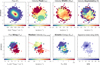 |
Fig. A.13. 3C 135, HEG, 1″ = 3.37 kpc. The black circle in the first panel has a diameter of 3 times the seeing of the observations; the dashed line in the second panel marks the radio position angle. We find a shape already observed in the 3C 033, an extended outflow characterized by two geometrically symmetrical lobes that cover ∼1.8″ (∼4 kpc). The lobe that extends in the NW is characterized by high negative velocities of the gas, with a maximum value that amount to ∼ − 1940 km s−1. In the other lobe that evolves towards SE the gas assumes lower positive velocities down to ∼570 km s−1. In the nucleus we measured a value of ∼290 km s−1 for the median velocity of the gas, anyway it is obscured preventing us to explore its energetic. Also for this source the radio image exceed the MUSE field of view. |
 |
Fig. A.14. 3C 180, HEG, 1″ = 3.37 kpc. The black circle in the first panel has a diameter of 3 times the seeing of the observations; the dashed line in the second panel marks the radio position angle. In the inner region the ionized gas is quite compact (up to ∼8.5 kpc from the nucleus), outside the central region (from ∼8.5 kpc to ∼15 kpc) the most distant gas is located in a larger area especially in the SE section, here the gas is dominated by high positive velocities that reach ∼2450 km s−1. This represents the maximum velocity reached by the outflow in the whole sample and also by the 3C 79. In this area we observe a thin segment of gas characterized by negative velocities. The NW area is dominated by the blue component. |
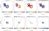 |
Fig. A.15. 3C 196.1, BLO, 1″ = 3.12 kpc. The black circle in the first panel has a diameter of 3 times the seeing of the observations; the dashed line in the second panel marks the radio position angle. The outflowing gas of this source is very compact, it is enclose in a region of radius ∼1.8 kpc. We observe the blue component of the [O III] with a maximum velocity of ∼ − 640 km s−1, unfortunately the image is not well resolved. In this case the MUSE field of view is larger than the radio image. |
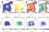 |
Fig. A.16. 3C 227, BLO, 1″ = 1.58 kpc. The black circle in the first panel has a diameter of 3 times the seeing of the observations; the dashed line in the second panel marks the radio position angle. the emission lines are detected in a compact but resolved region extending by ∼2.53 kpc from the nucleus. The ionized gas assumes negative velocities with the greatest value at −1920 km s−1 and the kinetic energy increases toward the center. The radio image terminate with two symmetrical hotspots exceeding the MUSE field of view. |
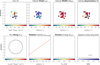 |
Fig. A.17. 3C 264, LEG, 1″ = 0.44 kpc. The black circle in the first panel has a diameter of 3 times the seeing of the observations; the dashed line in the second panel marks the radio position angle. |
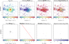 |
Fig. A.18. 3C 272.1, LEG, 1″ = 0.07 kpc. The black circle in the first panel has a diameter of 3 times the seeing of the observations; the dashed line in the second panel marks the radio position angle. |
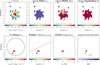 |
Fig. A.19. 3C 296, LEG, 1″ = 0.49 kpc. The black circle in the first panel has a diameter of 3 times the seeing of the observations; the dashed line in the second panel marks the radio position angle. |
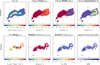 |
Fig. A.20. 3C 300, HEG, 1″ = 3.88 kpc. The black circle in the first panel has a diameter of 3 times the seeing of the observations; the dashed line in the second panel marks the radio position angle. This source shows an elliptical shape (the most extended f our sample) with a residual filamentary structure in the NE direction. The whole major axis of the ellipse has a length of ∼7.2″ (∼27.94 kpc), from its east end the emission lines extend beyond ∼12″ (∼9.31 kpc). The flux of the gas is major in correspondence with the nucleus and it peaks again at ∼14.25 kpc toward SW from the center. The outflow is mainly dominated by the blue component which maximum velocity is ∼ − 2160 km s−1. The red component of the gas is detected in the NE filaments with a velocity that arrives up to ∼1450 km s−1. The kinetic energy presents two peaks located in the same position as those of the flux. This double peak is probably a sign of two sources from which the outflow originates. |
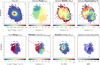 |
Fig. A.21. 3C 327, HEG, 1″ = 1.87 kpc. The black circle in the first panel has a diameter of 3 times the seeing of the observations; the dashed line in the second panel marks the radio position angle. Both component of the outflow are detected with a S/N above 100. To the west the ionized gas reaches positive velocities and in the opposite side negatives, achieving a maximum values by ∼1440 km s−1. The maps are well resolved, the energy peaks at the center then decreases more and more towards the external region (up to ∼3.74 kpc). |
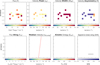 |
Fig. A.22. 3C 348, LEG, 1″ = 2.56 kpc. The black circle in the first panel has a diameter of 3 times the seeing of the observations; the dashed line in the second panel marks the radio position angle. |
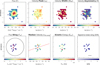 |
Fig. A.23. 3C 353, LEG, 1″ = 0.59 kpc. The black circle in the first panel has a diameter of 3 times the seeing of the observations; the dashed line in the second panel marks the radio position angle. |
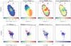 |
Fig. A.24. 3C 403, HEG, 1″ = 1.13 kpc. The black circle in the first panel has a diameter of 3 times the seeing of the observations; the dashed line in the second panel marks the radio position angle. The gas in outflow is mainly observed in a compact region. Its flux is concentrated into a radius of ∼1″. However, the gas also weakly extends in the NW-SE directions. The [O III] is blueshifted, reaching ∼ − 1940 km s−1. Its energy peaks in the nucleus where the median velocity of the gas is by ∼ − 430 km s−1. |
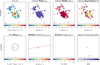 |
Fig. A.25. 3C 442, LEG, 1″ = 0.51 kpc. The black circle in the first panel has a diameter of 3 times the seeing of the observations; the dashed line in the second panel marks the radio position angle. |
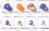 |
Fig. A.26. 3C 445, BLO, 1″ = 1.07 kpc. The black circle in the first panel has a diameter of 3 times the seeing of the observations; the dashed line in the second panel marks the radio position angle. In this source the outflowing gas assumes a flipped C shape extended by ∼8.60 kpc. The flux is approximately constant throughout the emission region while the velocity of the gas is major in the central area and decrease towards the two extremities. Here the emission lines are blueshifted showing velocities up to ∼ − 2160 km s−1 (the maximum velocity reached between the BLOs). At the distance of ∼1.50 kpc from this region a smaller redshifted area is detected with dimensions of ∼3 kpc, here the gas reaches velocities down to ∼1100 km s−1. The energy is higher in correspondence of the highest blueshifted velocities. |
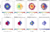 |
Fig. A.27. 3C 456, HEG, 1″ = 3.51 kpc. The black circle in the first panel has a diameter of 3 times the seeing of the observations; the dashed line in the second panel marks the radio position angle. The outflow maps of this source are very similar to the ones obtained for 3C 327. In this case the emission lines are just more extended: the outflow is enclosed into an area of radius ∼7.02 kpc. In the west region the redshifted component is detected (up to ∼1100 km s−1), in the east the blueshifted one (up to ∼ − 1900 km s−1). The image is clearly resolved, the energy peaks on the nucleus and decreases towards the border. |
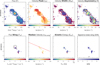 |
Fig. A.28. 3C 458, HEG, 1″ = 4.07 kpc. The black circle in the first panel has a diameter of 3 times the seeing of the observations; the dashed line in the second panel marks the radio position angle. |
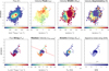 |
Fig. A.29. 3C 459, BLO, 1″ = 3.3 kpc. The black circle in the first panel of the bottom has a diameter of 3 times the seeing of the observations; the dashed red line in the second panel of the bottom marks the radio position angle. We presented detailed results obtained for this source in Balmaverde et al. (2018b). The outflowing gas is mainly confined in a region of radius ∼2.86 kpc. Here the gas has high negative velocities up to ∼ − 2040 km s−1. In the south there is a thin strip of redshifted gas. The maximum of the energy is found in correspondence with the blueshifted component of the ionized gas. |
All Tables
All Figures
|
Fig. 1. Comparison of the bolometric values derived from the [O III] luminosities with those obtained from 2 to 10 keV Chandra and 4400 Å HST optical luminosity using X-ray and optical bolometric corrections by Duras et al. (2020). |
| In the text | |
|
Fig. 2. Example of the [O III] emission-line profile (blue curve) of 3C 033 in the brightest spaxel of the image. The vertical orange line represents the velocity of the peak flux density (vp), and the green vertical lines show the 10th (v10) and 90th (v90) velocity percentiles, which are used for the definition of the velocity width of the line that contains 80% of the emission line flux (W80). In this spectrum the redshifted wing dominates, producing a positive value of the asymmetry (R > 0). The dotted red horizontal line is the continuum, linearly interpolated and subtracted. |
| In the text | |
|
Fig. 3. Nuclear spectra of 3C 015 and 3C 445. Left panel: observed [O III] emission line is shown (in blue) with the mirror image of the redshifted line (in black). Their difference (in red) reveals a blueshifted wing in the profile, with ionized gas that reaches high negative velocities. We masked the central region of the [O III] profile – at one-third of the maximum height of the emission line (grey region) – not considering the gas in ordered rotation. We measured the median velocity (v50) of the outflow measured on the blue-wing residual component. |
| In the text | |
|
Fig. 4. Comparison of the velocity measured at the 20th percentile of the whole [O III] line, v20, and of the median velocity (v50, wing) of the high-velocity wing on the nucleus. The dash-dotted line corresponds to a constant ratio of 1.6. This means that in our sample, v20 would overestimate the outflow velocity. |
| In the text | |
|
Fig. 5. Median velocity of the high-speed line wing (see text for details) as a function of the AGN bolometric luminosity. Green diamonds show HEGs, blue crosses show BLOs, red squares show LEGs, black circles show the spectroscopically unclassified sources, and the cyan circle represents the star forming galaxy. The empty symbols at the top of the figure represent sources without a detected line wing. The various classes show similar outflow velocities. |
| In the text | |
|
Fig. 6. Ratio of the [O III] luminosity of the nuclear outflowing gas with respect to the whole ionized gas in the galaxy nucleus vs. bolometric luminosity. |
| In the text | |
|
Fig. 7. Mass of ionized gas (top) and kinetic energy (bottom) of the nuclear outflows as a function of the AGN bolometric luminosity. The outflow mass and energy increase with the bolometric luminosity. The highest values are seen in BLOs. |
| In the text | |
|
Fig. 8. Spatially resolved maps of the parameters defined in Sect. 4 for 3C 033. The maps are centered on the nucleus of the source, identified by the [O III] peak luminosity. Top panelfrom left to right: (1) [O III] flux, (2) velocity peak (vp) of the [O III] emission line, (3) emission line width (W80), and (4) velocity asymmetry of the [O III] profile. Bottom panelfrom left to right: (1) flux of the outflowing gas isolated by the rotational component (Fw), the black circle has a diameter of three times the seeing of the observations; (2) median velocity of the outflowing gas (v50, wing), the dashed line marks the radio position angle; (3) kinetic energy of the [O III] emitting gas; and (4) S/N of the [O III] emission residing in the line wing. In all maps, pixels with an S/N < 5 have been discarded. |
| In the text | |
|
Fig. 9. Comparison of the [O III] luminosity of the high-velocity wing, measured in the whole outflow and in the nuclear region. The three BLOs these estimates are similar, but in the HEGs the outflow is dominated by its extended component. The dot-dashed line represents the 1:1 relation. |
| In the text | |
|
Fig. 10. Comparison of the outflow properties with the bolometric luminosity of the AGN (Lbol) and the Eddington ratio (Lbol/Ledd). Left panel: total kinetic energy of the outflow vs. Lbol. These quantities show a linear dependence. Right panel: velocity of the outflow vs. Lbol/Ledd. Most sources show velocities between ∼200 and ∼800 km s−1 with no clear trend with Lbol/Ledd or differences between the various spectroscopic classes. The open symbols correspond to sources without detected extended outflow. |
| In the text | |
|
Fig. 11. Top panel: outflow momentum boost divided by the AGN radiation momentum rate (Lbol/c) as a function of v50, wing. The dashed line marks the expectations for a momentum conserving outflow (ṖOF/Ṗrad = 1). Middle panel: wind mass outflow rate as a function of the AGN bolometric luminosity. Bottom panel: total outflow kinetic power vs. AGN bolometric luminosity. The grey points represent the data collected by Fiore et al. (2017); the dashed line represents the relation Ėkin = 0.5% Lbol, above which an energy-driven outflow can substantially heat or blow the galactic gas out. The open symbols correspond to sources without detected extended outflow. |
| In the text | |
|
Fig. 12. Comparison of the position angle of the extended outflow and the radio structure. |
| In the text | |
|
Fig. 13. Top panel: jet power, i.e., the energy per unit time carried from the radio jet vs. the nuclear bolometric luminosity. Bottom panel: Ėkin vs. Pjet. The dashed line represents the 1:1 relation. The jet should have an efficiency η ≈ 0.1−1 to sustain the kinetic power of the outflow. |
| In the text | |
|
Fig. A.1. Nuclear spectra of the 33 3C sources with a detection of the [O III] emission line. Superposed on the [O III] profile (blue) is the mirror image of the redshifted line (black). Their difference (red) reveals any line asymmetry. We estimated the median velocity (V50) of the asymmetric line wing and its flux (Fw), after masking the spectral region at one-third of the maximum height of the profile (grey region). |
| In the text | |
|
Fig. A.1. continued. |
| In the text | |
|
Fig. A.2. 3C 015, LEG, 1″ = 1.36 kpc. The black circle in the first panel has a diameter of 3 times the seeing of the observations; the dashed line in the second panel marks the radio position angle. Its nuclear outflow appear to be confined in a circular region of radius ∼0.98 kpc and having a blue-shifted component peaking at ∼ − 890 km s−1. The outflow is well resolved enabling us to observe a kinetic energy increasing towards the center. |
| In the text | |
|
Fig. A.3. 3C 017, BLO, 1″ = 3.37 kpc. The black circle in the first panel has a diameter of 3 times the seeing of the observations; the dashed line in the second panel marks the radio position angle. The outflowing gas is moving toward us reaching negative values of velocity. Unfortunately its compactness (the upper limit of its extension from the center is ∼1.68 kpc) prevent us from producing a well resolved map of its kinetic energy. The ionized gas achieves a velocity up to ∼ − 1100 km s−1. |
| In the text | |
|
Fig. A.4. 3C 018, BLO, 1″ = 3.00 kpc. The black circle in the first panel has a diameter of 3 times the seeing of the observations; the dashed line in the second panel marks the radio position angle. The ionized gas appears well resolved, reaching high negative velocities up to ∼ − 1120 km s−1. The kinetic energy gradually decrease from the central nucleus to the edge (∼2.52 kpc). |
| In the text | |
|
Fig. A.5. 3C 029, LEG, 1″ = 0.88 kpc. The black circle in the first panel has a diameter of 3 times the seeing of the observations; the dashed line in the second panel marks the radio position angle. Similarly to 3C 017 the emission line are only few extended and not well resolved. The maximum extension is reached in the SW region at ∼0.20 kpc from the nucleus. We observe only the blue component of the outflow. |
| In the text | |
|
Fig. A.6. 3C 033, HEG, 1″ = 1.14 kpc. The black circle in the first panel has a diameter of 3 times the seeing of the observations; the dashed line in the second panel marks the radio position angle. We observe an outflow symmetrically extended towards the NW and the SE directions out to ∼3.4″ (∼3.88 kpc) from the nucleus. In the NW region the gas assumes positive velocities (up to ∼1800 km s−1) and in the SE negative values (up to ∼2000 km s−1), in both cases they slowly decrease along the maximum extension. The kinetic energy grows from the most external regions close to the center, reaching the maximum values at ∼1.00 kpc from the nucleus and decreasing again approaching the center. This is due to our field of view in which the nucleus is obscured by the torus surrounding the central engine. In fact the highest values of S/N are measured in the same area in which the energy gets the greatest values. |
| In the text | |
|
Fig. A.7. 3C 040, LEG, 1″ = 0.36 kpc. The black circle in the first panel has a diameter of 3 times the seeing of the observations; the dashed line in the second panel marks the radio position angle. |
| In the text | |
|
Fig. A.8. 3C 063, HEG, 1″ = 1.36 kpc. The black circle in the first panel has a diameter of 3 times the seeing of the observations; the dashed line in the second panel marks the radio position angle. The gas in outflow shows a quite circular shape with a radius of ∼1.14 kpc with a elongation in the SE direction (∼ out to 2.12 kpc). We observe just the blue component of the [O III] with a velocity down to ∼1900 km s−1. |
| In the text | |
|
Fig. A.9. 3C 079, HEG, 1″ = 3.75 kpc. The black circle in the first panel has a diameter of 3 times the seeing of the observations; the dashed line in the second panel marks the radio position angle. The outflow gas is confined in a circular region of radius ∼7.5 kpc, from here two filamentary structures extend beyond ∼36 kpc and ∼26 kpc respectively towards NE and SW. The filaments appears as the division axis between the gas launched in our direction (upper area) and the one in the opposite side (bottom area). The central region of the source is obscured, prevent us to observe the energetic of the nucleus. The maximum velocity achieved by the [O III] is ∼2450 km s−1, that represents the maximum velocity reached by the outflow in the whole sample and also by the 3C 180. |
| In the text | |
|
Fig. A.10. 3C 088, LEG, 1″ = 0.60 kpc. The black circle in the first panel has a diameter of 3 times the seeing of the observations; the dashed line in the second panel marks the radio position angle. The source is well resolved, the kinetic energy of the gas increases in the inner part and its velocities are negative out to ∼ − 1360 km s−1. The outflow not expands beyond 0.72 kpc from the nucleus. |
| In the text | |
|
Fig. A.11. 3C 098, LEG, 1″ = 0.60 kpc. The black circle in the first panel has a diameter of 3 times the seeing of the observations; the dashed line in the second panel marks the radio position angle. The MUSE field-of-view covers only ∼1/4 of the extension of the radio source. Even if the map is not well resolved we can see that the ionized gas of the outflow reaching negative velocities beyond ∼2000 km s−1 and it expands into an irregular structure. |
| In the text | |
|
Fig. A.12. 3C 105, BLO, 1″ = 1.63 kpc. The black circle in the first panel has a diameter of 3 times the seeing of the observations; the dashed line in the second panel marks the radio position angle. |
| In the text | |
|
Fig. A.13. 3C 135, HEG, 1″ = 3.37 kpc. The black circle in the first panel has a diameter of 3 times the seeing of the observations; the dashed line in the second panel marks the radio position angle. We find a shape already observed in the 3C 033, an extended outflow characterized by two geometrically symmetrical lobes that cover ∼1.8″ (∼4 kpc). The lobe that extends in the NW is characterized by high negative velocities of the gas, with a maximum value that amount to ∼ − 1940 km s−1. In the other lobe that evolves towards SE the gas assumes lower positive velocities down to ∼570 km s−1. In the nucleus we measured a value of ∼290 km s−1 for the median velocity of the gas, anyway it is obscured preventing us to explore its energetic. Also for this source the radio image exceed the MUSE field of view. |
| In the text | |
|
Fig. A.14. 3C 180, HEG, 1″ = 3.37 kpc. The black circle in the first panel has a diameter of 3 times the seeing of the observations; the dashed line in the second panel marks the radio position angle. In the inner region the ionized gas is quite compact (up to ∼8.5 kpc from the nucleus), outside the central region (from ∼8.5 kpc to ∼15 kpc) the most distant gas is located in a larger area especially in the SE section, here the gas is dominated by high positive velocities that reach ∼2450 km s−1. This represents the maximum velocity reached by the outflow in the whole sample and also by the 3C 79. In this area we observe a thin segment of gas characterized by negative velocities. The NW area is dominated by the blue component. |
| In the text | |
|
Fig. A.15. 3C 196.1, BLO, 1″ = 3.12 kpc. The black circle in the first panel has a diameter of 3 times the seeing of the observations; the dashed line in the second panel marks the radio position angle. The outflowing gas of this source is very compact, it is enclose in a region of radius ∼1.8 kpc. We observe the blue component of the [O III] with a maximum velocity of ∼ − 640 km s−1, unfortunately the image is not well resolved. In this case the MUSE field of view is larger than the radio image. |
| In the text | |
|
Fig. A.16. 3C 227, BLO, 1″ = 1.58 kpc. The black circle in the first panel has a diameter of 3 times the seeing of the observations; the dashed line in the second panel marks the radio position angle. the emission lines are detected in a compact but resolved region extending by ∼2.53 kpc from the nucleus. The ionized gas assumes negative velocities with the greatest value at −1920 km s−1 and the kinetic energy increases toward the center. The radio image terminate with two symmetrical hotspots exceeding the MUSE field of view. |
| In the text | |
|
Fig. A.17. 3C 264, LEG, 1″ = 0.44 kpc. The black circle in the first panel has a diameter of 3 times the seeing of the observations; the dashed line in the second panel marks the radio position angle. |
| In the text | |
|
Fig. A.18. 3C 272.1, LEG, 1″ = 0.07 kpc. The black circle in the first panel has a diameter of 3 times the seeing of the observations; the dashed line in the second panel marks the radio position angle. |
| In the text | |
|
Fig. A.19. 3C 296, LEG, 1″ = 0.49 kpc. The black circle in the first panel has a diameter of 3 times the seeing of the observations; the dashed line in the second panel marks the radio position angle. |
| In the text | |
|
Fig. A.20. 3C 300, HEG, 1″ = 3.88 kpc. The black circle in the first panel has a diameter of 3 times the seeing of the observations; the dashed line in the second panel marks the radio position angle. This source shows an elliptical shape (the most extended f our sample) with a residual filamentary structure in the NE direction. The whole major axis of the ellipse has a length of ∼7.2″ (∼27.94 kpc), from its east end the emission lines extend beyond ∼12″ (∼9.31 kpc). The flux of the gas is major in correspondence with the nucleus and it peaks again at ∼14.25 kpc toward SW from the center. The outflow is mainly dominated by the blue component which maximum velocity is ∼ − 2160 km s−1. The red component of the gas is detected in the NE filaments with a velocity that arrives up to ∼1450 km s−1. The kinetic energy presents two peaks located in the same position as those of the flux. This double peak is probably a sign of two sources from which the outflow originates. |
| In the text | |
|
Fig. A.21. 3C 327, HEG, 1″ = 1.87 kpc. The black circle in the first panel has a diameter of 3 times the seeing of the observations; the dashed line in the second panel marks the radio position angle. Both component of the outflow are detected with a S/N above 100. To the west the ionized gas reaches positive velocities and in the opposite side negatives, achieving a maximum values by ∼1440 km s−1. The maps are well resolved, the energy peaks at the center then decreases more and more towards the external region (up to ∼3.74 kpc). |
| In the text | |
|
Fig. A.22. 3C 348, LEG, 1″ = 2.56 kpc. The black circle in the first panel has a diameter of 3 times the seeing of the observations; the dashed line in the second panel marks the radio position angle. |
| In the text | |
|
Fig. A.23. 3C 353, LEG, 1″ = 0.59 kpc. The black circle in the first panel has a diameter of 3 times the seeing of the observations; the dashed line in the second panel marks the radio position angle. |
| In the text | |
|
Fig. A.24. 3C 403, HEG, 1″ = 1.13 kpc. The black circle in the first panel has a diameter of 3 times the seeing of the observations; the dashed line in the second panel marks the radio position angle. The gas in outflow is mainly observed in a compact region. Its flux is concentrated into a radius of ∼1″. However, the gas also weakly extends in the NW-SE directions. The [O III] is blueshifted, reaching ∼ − 1940 km s−1. Its energy peaks in the nucleus where the median velocity of the gas is by ∼ − 430 km s−1. |
| In the text | |
|
Fig. A.25. 3C 442, LEG, 1″ = 0.51 kpc. The black circle in the first panel has a diameter of 3 times the seeing of the observations; the dashed line in the second panel marks the radio position angle. |
| In the text | |
|
Fig. A.26. 3C 445, BLO, 1″ = 1.07 kpc. The black circle in the first panel has a diameter of 3 times the seeing of the observations; the dashed line in the second panel marks the radio position angle. In this source the outflowing gas assumes a flipped C shape extended by ∼8.60 kpc. The flux is approximately constant throughout the emission region while the velocity of the gas is major in the central area and decrease towards the two extremities. Here the emission lines are blueshifted showing velocities up to ∼ − 2160 km s−1 (the maximum velocity reached between the BLOs). At the distance of ∼1.50 kpc from this region a smaller redshifted area is detected with dimensions of ∼3 kpc, here the gas reaches velocities down to ∼1100 km s−1. The energy is higher in correspondence of the highest blueshifted velocities. |
| In the text | |
|
Fig. A.27. 3C 456, HEG, 1″ = 3.51 kpc. The black circle in the first panel has a diameter of 3 times the seeing of the observations; the dashed line in the second panel marks the radio position angle. The outflow maps of this source are very similar to the ones obtained for 3C 327. In this case the emission lines are just more extended: the outflow is enclosed into an area of radius ∼7.02 kpc. In the west region the redshifted component is detected (up to ∼1100 km s−1), in the east the blueshifted one (up to ∼ − 1900 km s−1). The image is clearly resolved, the energy peaks on the nucleus and decreases towards the border. |
| In the text | |
|
Fig. A.28. 3C 458, HEG, 1″ = 4.07 kpc. The black circle in the first panel has a diameter of 3 times the seeing of the observations; the dashed line in the second panel marks the radio position angle. |
| In the text | |
|
Fig. A.29. 3C 459, BLO, 1″ = 3.3 kpc. The black circle in the first panel of the bottom has a diameter of 3 times the seeing of the observations; the dashed red line in the second panel of the bottom marks the radio position angle. We presented detailed results obtained for this source in Balmaverde et al. (2018b). The outflowing gas is mainly confined in a region of radius ∼2.86 kpc. Here the gas has high negative velocities up to ∼ − 2040 km s−1. In the south there is a thin strip of redshifted gas. The maximum of the energy is found in correspondence with the blueshifted component of the ionized gas. |
| In the text | |
Current usage metrics show cumulative count of Article Views (full-text article views including HTML views, PDF and ePub downloads, according to the available data) and Abstracts Views on Vision4Press platform.
Data correspond to usage on the plateform after 2015. The current usage metrics is available 48-96 hours after online publication and is updated daily on week days.
Initial download of the metrics may take a while.