| Issue |
A&A
Volume 653, September 2021
|
|
|---|---|---|
| Article Number | A155 | |
| Number of page(s) | 17 | |
| Section | Extragalactic astronomy | |
| DOI | https://doi.org/10.1051/0004-6361/202040009 | |
| Published online | 28 September 2021 | |
Faint polarised sources in the Lockman Hole field at 1.4 GHz⋆
1
Ruhr University Bochum, Faculty of Physics and Astronomy, Astronomical Institute (AIRUB), Universitätsstrasse 150, 44780 Bochum, Germany
e-mail: berger@astro.rub.de
2
Ruhr University Bochum, Faculty of Physics and Astronomy, Astronomical Institute (AIRUB), German Centre for Cosmological Lensing, Universitätsstrasse 150, 44780 Bochum, Germany
3
INAF – Instituto di Radioastronomia, via Gobletti 101, 40126 Bologna, Italy
Received:
27
November
2020
Accepted:
21
June
2021
Context. In the context of structure formation and galaxy evolution, the contribution of magnetic fields is not well understood. Feedback processes originating from active galactic nucleus (AGN) activity and star formation can be actively influenced by magnetic fields, depending on their strength and morphology. One of the best tracers of magnetic fields is polarised radio emission. Tracing this emission over a broad redshift range therefore allows an investigation of these fields and their evolution.
Aims. We aim to study the nature of the faint, polarised radio source population whose source composition and redshift dependence contain information about the strength, morphology, and evolution of magnetic fields over cosmic timescales.
Methods. We use a 15-pointing radio continuum L-band mosaic of the Lockman Hole, observed in full polarisation, generated from archival data of the Westerbork Synthesis Radio Telescope. The data were analysed using the rotation measure synthesis technique. We achieved a noise of 7 μJy beam−1 in polarised intensity, with a resolution of 15″. Using infrared and optical images and source catalogues, we were able to cross-identify and determine redshifts for one-third of our detected polarised sources.
Results. We detected 150 polarised sources, most of which are weakly polarised with a mean fractional polarisation of 5.4%. No source was found with a fractional polarisation higher than 21%. With a total area of 6.5 deg2 and a detection threshold of 6.25σ, we find 23 polarised sources per deg2. Based on our multi-wavelength analysis, we find that our sample consists of AGN only. We find a discrepancy between archival number counts and those present in our data, which we attribute to sample variance (i.e. large-scale structures). Considering the absolute radio luminosity, we find a general trend of increased probability of detecting weak sources at low redshift and strong sources at high redshift. We attribute this trend to a selection bias. Further, we find an anti-correlation between fractional polarisation and redshift for our strong-source sample at z ≥ 0.6.
Conclusions. A decrease in the fractional polarisation of strong sources with increasing redshift cannot be explained by a constant magnetic field and electron density over cosmic scales; however, the changing properties of cluster environments over cosmic time may play an important role. Disentangling these two effects requires deeper and wider polarisation observations as well as better models of the morphology and strength of cosmic magnetic fields.
Key words: magnetic fields / polarization / cosmology: observations / galaxies: active / radio continuum: general
Full Table A.5 is only available at the CDS via anonymous ftp to cdsarc.u-strasbg.fr (130.79.128.5) or via http://cdsarc.u-strasbg.fr/viz-bin/cat/J/A+A/653/A155
© ESO 2021
1. Introduction
Feedback processes within star-forming galaxies and active galactic nuclei (AGN) are known to be the main drivers of the enrichment of the intergalactic medium. While star-forming galaxies are more numerous than AGN by two orders of magnitude, AGN are much more energetic. It is therefore a matter of debate as to which of these two object classes dominates the feedback process.
It is known that AGN and star-formation activity correlate up to redshifts of z ∼ 1.5 (Boyle & Terlevich 1998; Wall 1998), but discrepancies exist at higher redshifts (Wall et al. 2005). However, many analyses of sources at higher redshifts are biased towards more massive and active sources (Taniguchi 2004; Fiore et al. 2012), such as starburst objects or those in the Fanaroff-Riley (FR) II category (Fanaroff & Riley 1974). As a result, the contribution of the more numerous, radio-quiet (and therefore faint) sources remains unknown. A detailed understanding of the faint radio source population, and the underlying physical processes dominating feedback, is therefore indispensable when attempting to explain galaxy formation and evolution overall.
Understanding the influence of magnetic fields on large scales, and how they evolve into the regular magnetic field structures we see in the nearby Universe today, is an open question in current observational and theoretical astronomy. While we can directly observe the morphology (and estimate the strength) of magnetic fields in nearby objects (Beck 2015; Blandford et al. 2019), the necessary information for evolutionary studies over cosmic timescales can only be provided statistically using samples of sources that span cosmic timescales.
One of the best tracers of magnetic field strength and morphology is total and polarised radio synchrotron emission: We can examine the integrated quantities of the magnetic field via the total power emission and analyse the field’s degree of ordering and geometry using the polarised emission. As such, the faint polarised radio sky provides a direct window into the evolution of the magnetic field over cosmic timescales. Using statistically significant samples of polarised radio sources allows us to simultaneously trace their characteristics as a population (Lamee et al. 2016; Farnes et al. 2014), observe the possible changes they undergo during their evolution, and explore the structure of the intervening cosmic magnetic field (Vernstrom et al. 2018).
Most past studies of polarised radio sources were based on single objects or small targeted samples. Upcoming wide-field radio surveys, which observe both total intensity and polarisation, are now providing statistical constraints on the polarisation properties of faint radio-selected AGN and star-forming objects.
Deep field polarisation studies at 1.4 GHz, down to detection thresholds of around 50 μJy beam−1 and over areas of several square degrees, have been conducted within several projects (Taylor et al. 2007; Grant et al. 2010; Subrahmanyan et al. 2010; Hales et al. 2014a). Rudnick & Owen (2014) made even deeper observations, down to a noise level of ∼3 μJy beam−1, but for a smaller survey area of approximately 0.3 deg2.
Total power source counts show that below flux densities of 0.5 − 1 mJy star-forming galaxies become progressively dominant over AGN, which constitute the majority of the sources at higher flux densities (Hopkins et al. 2003; Mignano et al. 2008). These differences in structure, as well as in the source nature, likely introduce differences into the polarisation properties of the faint source population compared to their bright population counterparts (Stil et al. 2014). In contrast to this, the faint, polarised sky (down to the microjansky level) is still dominated by AGN (Hales et al. 2014a). In addition, the polarisation properties of AGN have been found to differ depending on their morphology (Conway et al. 1977) and spectral properties (Mesa et al. 2002; Tucci et al. 2004).
Studies by Mesa et al. (2002), Tucci et al. (2004), Taylor et al. (2007), and Grant et al. (2010) observed an anti-correlation between the degree of linear polarisation and the total intensity of the faint extra-galactic radio source population at 1.4 GHz. It was supposed by Hales et al. (2014a) that this correlation is not caused by the physical properties of the sources but rather originates from the incompleteness affecting the faintest sources in the sample. In agreement with this, Stil et al. (2014) observed a much more gradual trend when stacking polarised sources in the NRAO VLA Sky Survey (NVSS; Condon et al. 1998).
The Lockman Hole (Lockman et al. 1986) is one of the best studied regions of the sky over a multitude of wavelength regimes, which has led to an extensive multi-band coverage of the field. Here we briefly describe the observations we used for this publication. A complete description of all available data in the field is available in Prandoni et al. (2018). The Lockman Hole has a low infrared (IR) background of about 0.38 MJy sr−1 at 100 μm (Lonsdale et al. 2003), which makes it well suited for IR observations. Thus, about 12 deg2 of the field were observed with the Spitzer Space Telescope (Werner et al. 2004) as part of the Spitzer Wide-area Infrared Extragalactic (SWIRE) survey (Lonsdale et al. 2003) at 3.6, 4.5, 5.8, 8.0, 24, 70, and 160 μm. The Lockman Hole was also observed in the far infrared (FIR) as part of the Herschel Multi-tiered Extragalactic Survey (Oliver et al. 2012), in the ultraviolet regime by the Galaxy Evolution Explorer (GALEX) GR6Plus7 (Martin et al. 2005), and as part of the Sloan Digital Sky Survey (SDSS) Data Release 7 (DR7; Abolfathi et al. 2018). The Lockman Hole is also part of a deep optical weak-lensing analysis by Tudorica et al. (2017), who used data from the Canada-France-Hawaii Telescope (CFHT) in five optical bands (ugriz) and measured photometric redshifts.
A variety of radio surveys cover limited areas (< 1 deg2) within the Lockman Hole region. Recently, wider radio coverage has been obtained with the Low-Frequency Array (LOFAR) at 150 MHz (Mahony et al. 2016) and with the Westerbork Synthesis Radio Telescope (WSRT) at 1.4 GHz. The WSRT mosaic covers ∼6.6 deg2 down to 11 μJy beam−1 in root-mean-squared (RMS) deviation (Prandoni et al. 2018). Both datasets were, however, only analysed in total power radio continuum; this paper aims to study the polarisation properties of the field at 1.4 GHz. Deep, wide-area radio surveys represent excellent probes of magnetic fields over cosmologically significant redshift intervals.
The paper is organised as follows. In Sect. 2 we present our data and the data reduction strategy to obtain a mosaic in polarised intensity. In Sect. 3 we describe our source identification and catalogue creation. Section 4 covers the cross-identification procedures with other source catalogues at other wavelengths. This information is used in Sect. 5 for the classification of the polarised sources. In Sect. 6 we present our results. A part of our results are analysed with respect to the cosmic evolution of magnetic fields in Sect. 7. Section 8 gives a discussion of these magnetic fields, and our summary is presented in Sect. 9.
2. Data
This study is based on the WSRT observations of the Lockman Hole field at 1.4 GHz (Prandoni et al. 2018). The data consist of 16 individual pointings, each observed for a full synthesis of 12 hrs between December 2006 and January 2007. Individual pointing centres are given in Table A.1. The centre of the mosaic was chosen to be at RA = 10:53:16.6; Dec = +58:01:15 (J2000).
Each dataset was recorded over a full bandwidth of 160 MHz organised in eight 20 MHz sub-bands with 64 channels each. The channel width is 312 kHz, the central sub-band frequencies are 1451, 1422, 1411, 1393, 1371, 1351, 1331 and 1311 MHz. The data were recorded in all four linear correlations (XX, XY, YX, and YY) and thus contains full polarisation information. The total power calibration and imaging was already performed by Prandoni et al. (2018).
The standard flux calibrator source 3C48 was observed for 900 s before all 16 target fields. The polarisation calibrator 3C138 was also observed for 900 s before the target fields, but was missing for Pointing 12, which we therefore excluded from the data reduction; inclusion of these data would have resulted in inconsistent polarisation calibration within parts of the dataset.
2.1. Data reduction
For the data reduction we used a combination of the Astronomical Image Processing System (AIPS; Greisen 2010), the Common Astronomy Software Application (CASA) package (McMullin et al. 2007) and the Multichannel Image Reconstruction Image Analysis and Display (MIRIAD; Sault et al. 1995) software package. First AIPS was used to apply the system temperatures, after which we converted the data into the CASA MS-format to inspect the data for radio frequency interference (RFI). We used AOFlagger (Offringa et al. 2010) to perform an automatic flagging of RFI within our dataset. To allow an easier identification of RFI we applied a preliminary bandpass calibration, thereby mitigating the rapid roll-off effect of the receiver response curve at the edges of the frequency bands. This bandpass, however, was not used for any further calibration steps. All data were additionally inspected by eye to flag remaining RFI using RFI GUI (the graphical front-end of AOFlagger). Afterwards, the final bandpass calibration was applied, as well as the gain and polarisation leakage calibration, using the unpolarised calibrator source 3C48. The calibrator 3C138 was used to calibrate the polarisation angle. Models for 3C48 and 3C138 were taken from Perley & Butler (2017). The cross-calibration was then performed on a per-channel basis following the procedure described in Adebahr et al. (2013), to minimise polarisation leakage. After the cross-calibration in CASA, we imported the target data into MIRIAD for imaging and full polarimetric self-calibration using the MIRIAD task GPSCAL. To avoid including artificial sources in the self-calibration process, we created masks for every pointing in total power and used them for cleaning all four Stokes parameters. The self-calibration and imaging process was performed on each sub-band for each pointing individually. We consecutively decreased the solution interval from 20 min (for the first self-calibration cycle) to 30 s (for the last). We excluded short baselines in the first self-calibration cycles and extended the (u, v)-range to include all baselines for the later ones. Lastly, we used phase-only solutions for the first iterations and, in the final step, included both amplitude and phase calibration for data where enough signal-to-noise was available.
Using a joint deconvolution approach we generated cleaned image cubes of all 15 pointings in Stokes Q and U. For each sub-band the data of eight adjacent channels was imaged together resulting in an averaged channel width of 2.5 MHz each. Averaging the data to a coarser frequency resolution before imaging has the advantage that the individual Stokes Q and U images can be cleaned to greater depth, and therefore artefacts from sidelobes can be minimised. The resulting 128 images (64 for each of the two Stokes parameters) covering the whole bandwidth of the observation were cleaned and independently primary-beam-corrected using the standard primary beam correction for the WSRT: cos6(cνr), where c = 68 at L-band frequencies, ν is the frequency in GHz, and r the distance from the pointing centre in radians.
2.2. Rotation measure synthesis
To mitigate the effect of bandwidth depolarisation we used the rotation measure (RM) synthesis technique (Brentjens & de Bruyn 2005). The resulting parameters for the RM synthesis are: δψ = 328.46 rad m−2, max-scale = 74.46 rad m−2 and ψmax = 10095.57 rad m−2, where δψ represents the resolution in Faraday space, max-scale the maximum observable width of a polarised structure in Faraday space and ψmax the maximum observable Faraday depth before polarised emission becomes depolarised due to bandwidth smearing effects. Frequency averaging only influences the maximum observable RM and the recovered polarised intensity in case of sources exceeding this limit. For this study we expect our sources to have maximum RMs of several hundred, such that we should not lose any relevant information due to the applied averaging.
The Faraday cube was sampled between −1024 rad m−2 and 1024 rad m−2 using a sampling interval of 4 rad m−2. To derive the polarised emission map from the cube, we fitted a parabola to the first peak along the Faraday axis at any values exceeding 5σ. The polarised emission is determined by the peak value of the parabola. This was done to compensate for the limited sampling rate. Our final polarised emission map reaches a central RMS of 7 μJy beam−1. The map is shown in Fig. 1.
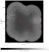 |
Fig. 1. 1.4 GHz polarised intensity mosaic from 15 overlapping pointings observed with the WSRT. The grey scale shows the polarised flux density. The centres of the individual pointing positions are marked with the pointing numbers in red. Pointing 12 was not used in this analysis, as discussed in Sect. 2. |
3. Source detection
3.1. pyBDSF
We used pyBDSF (Mohan & Rafferty 2015) to create a catalogue of polarised sources. To account for the higher RMS close to the edges of the mosaic we derived a local RMS map by using the adaptiv_rms_box option with 60 px boxes with a step size of 20 px. As a source detection threshold we used 6.25σ, which is comparable to a Gaussian threshold of 5.33σ (Hales et al. 2014a). The threshold for the island boundary was set to 5σ. This resulted in a catalogue containing 178 components. To acquire a measure of the complete polarised flux of each source, we summed the flux densities of the associated components (as identified by pyBDSF), which resulted in a catalogue of 154 polarised sources. The summation was done with the measurements of pyBDSF on the polarised intensity map. We note that following Sect. 3.3 the final published catalogue contains 150 sources.
3.2. Fractional polarisation
To calculate the fractional polarisation values (Π = PI/I, where PI is the polarised intensity and I the total intensity) of every source we also created an image in total intensity. Importantly, we opted to generate a bespoke total intensity map using our reduction strategy described previously (rather than simply use the map presented in Prandoni et al. 2018), in order to ensure consistency between our polarised and total intensity maps. To this end we assembled a mosaic for each sub-band and stacked the individual sub-band images using the MIRIAD task IMCOMB, with an inverse square weighting of the noise in the individual images. The resulting mosaic has a central RMS of 30 μJy beam−1. Again for the sake of consistency, we once more used pyBDSF for our source extraction. In this case we applied a detection threshold of 5σ to create a catalogue of the total power components, and the threshold for the island boundary was set to 3σ. To create a source catalogue we again summed the total flux densities of the associated components, resulting in a catalogue of 1708 sources, following the same strategy as for the polarised catalogue. This leads to a source density of about 262/deg2, which is in good agreement with other deep field studies with comparable noise levels (e.g., Taylor et al. 2007; Hales et al. 2014b; Subrahmanyan et al. 2010). Finally, we note that the aim of the image generation in total intensity was not to optimise the detection and flux measurement for all possible sources within the field, but rather to obtain an estimate of the total intensity fluxes for each of our polarised sources that is consistent with our polarised measurements. As such, we prioritise consistency over absolute signal-to-noise, and are therefore not concerned that our resulting total intensity maps have higher central RMS than the equivalent map produced by Prandoni et al. (2018).
We cross-matched the component catalogue in polarised intensity with our component catalogue in total intensity, using a matching radius of 30″; that is, twice the 15″ beam present in the polarised intensity map. All matches were confirmed or rejected via visual inspection. In case of some complex polarised sources, individual parts of the sources were identified as separate objects. To mitigate this effect, in cases where these could be associated (by visual inspection) with the same total power source, the previously individual components were again manually summed together into a single combined source for further analysis. For two of our polarised sources, no total intensity counterpart was found. The visual inspection of these sources showed that, due to reduction artefacts in the total intensity image, pyBDSF was not able to detect these sources. These sources were therefore resigned to inherit the total flux measurements of Prandoni et al. (2018), and were marked as such within our catalogue.
3.3. Instrumental polarisation
We checked for the influence of artificial instrumental polarisation by imaging four overlapping pointings. This allowed us to determine the polarised intensity for the same sources with different distances and directions from their pointing centres. pyBDSF was again used for source identification and flux measurements. By cross-matching the resulting catalogues of the individual pointings with each other and with our catalogue, we found that the measured polarised flux densities are consistent within their individual uncertainties. In addition, we found no sources that were detected in an individual pointing and not detected in the mosaic, nor any sources that were detected in one individual pointing and not in another (overlapping) pointing.
Since we therefore have no evidence for additional instrumental polarisation, we concluded to use a conservative cutoff of 0.5% in fractional polarisation for considering sources as physically polarised. We excluded all sources with a fractional polarisation lower than this cutoff limit. This criterion excluded 4 sources from further analysis, resulting in a remaining sample of 150 sources with 172 components, this is a polarised source density of 23/deg2. The catalogue is given in the Appendix A. Most sources were found to have modest polarisation, with a mean fractional polarisation Π = 5.4%. The highest degree of polarisation found was 21%.
4. Cross-identification
Using the catalogue from Helfand et al. (2015) we cross-matched our total-intensity sources with their FIRST counterparts to verify our astrometric calibration. To establish the calibration accuracy, we restrict this comparison to point-sources within our sample, which are selected using the S-Code ‘S’ from pyBDSF. We find a median offset of ΔRA = 0.26″ ± 2.34″ and ΔDec = 2.42″ ± 2.99″ of our coordinates compared to the FIRST coordinates (Fig. 2). A general offset of the FIRST coordinates was previously noticed by Grant et al. (2010), who found an average offset of ΔRA = 0.5″ ± 0.2″ and ΔDec = 0.4″ ± 0.2″. To minimise the influence of such an astrometric offset, we additionally check any subsequent cross-matching with other catalogues individually by eye.
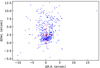 |
Fig. 2. Differences in the source positions between our observations and the FIRST catalogue. The red cross shows the mean ΔRA and ΔDec of the scatter, where the uncertainties are the standard deviation. |
4.1. Spectral index
To explore the spectral properties of the polarised sources, we used the catalogue of Mahony et al. (2016) who determined the spectral index of sources in the Lockman Hole field using LOFAR 150 MHz and WSRT 1.4 GHz observations. For cross-matching our sources with their catalogue, we used the coordinates of the sources in total power and a search radius of 15″. The best match for every source was then additionally inspected by eye. For four polarised sources no LOFAR counterpart was found. In Fig. 3 we show a histogram of the total power spectral indices of our polarised sources. The histogram shows the same source distribution as Mahony et al. (2016) show in their paper (Fig. 15) for their whole Lockman Hole sample. The median spectral index of our sample is α = −0.8 ± 0.07, which is consistent, within uncertainties, with the median spectral index from Mahony et al. (2016) of α = −0.78 ± 0.015. Throughout this publication we define the spectral index α using the relation S ∝ να.
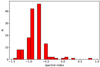 |
Fig. 3. Histogram of the total power spectral indices for our polarised sources. The spectral indices between 150 MHz and 1.4 GHz are taken from Mahony et al. (2016). |
4.2. Infrared cross-identification
Following the same procedure as presented by Hales et al. (2014a), we used the FIR-radio correlation (FRC), plus mid-infrared (MIR) colours, to distinguish galaxies dominated by star formation – that is, star-forming galaxies (SFGs) – from AGN. As part of the SWIRE survey the Lockman Hole was observed with the InfraRed Array Camera (IRAC; Fazio et al. 2004) as well as with the Multiband Imaging Photometer for Spitzer (MIPS; Rieke et al. 2004). IRAC observes in four MIR bands, with effective wavelengths of 3.6, 4.5, 5.8 and 8.0 μm. MIPS observes in the FIR bands at 24, 70 and 160 μm. The data were taken from the online NASA/Infrared Processing and Analysis Center (IPAC) science archive1. For cross-identification, we first determined the best matching source within a radius of 15″ of our total-intensity sources. The cross-matches of all polarised sources were than checked by eye for verification, using the polarised and total intensity maps and the SWIRE images. After this cross-matching and visual inspection, we found 35 sources were detected in all four IRAC bands, and 14 of these were also detected at 24 μm in MIPS. Four sources were detected at 24 μm but not in all IRAC bands. In total we found SWIRE counterparts for 39 of our polarised sources.
4.3. Photometric redshift
In order to investigate the redshift dependence of characteristics within our polarised source population, we cross-matched our sample with the catalogue from Tudorica et al. (2017), who used deep five-band optical imaging of the Lockman Hole from CFHT to derive photometric redshifts. A direct cross-match between our radio catalogue and the aforementioned optical catalogue from Tudorica et al. (2017) did not give reliable results, as within one beam we found multiple possible optical counterparts. To remedy this problem, we sought to use the higher resolution infrared information as a bridge between our optical and radio catalogues. The brightness correlation between optical and radio wavelengths is weak for galaxies; however, there is a significant correlation between sources radio and their infrared fluxes. As a result, sources dominating the flux within our radio beam should therefore also be the brightest in the infrared images. Furthermore, the MIR images are sufficiently high resolution such that optical-FIR cross-matches are unique; both the optical and FIR imaging have resolutions better than 2″in full width at half maximum (FWHM) of the point-spread function (PSF). Therefore, assuming the radio-MIR correlation holds, we are able to uniquely map optical counterparts to our radio emission via the high-resolution SWIRE imaging. Additionally, we visually inspected each source, using our polarised and total intensity map, the SWIRE infrared images, and the optical images, to identify false associations.
Sources that showed clear AGN jet structure in our total intensity map but were not detected by SWIRE were used to co-locate the central host galaxy. This was done by eye and enabled us to cross-identify two additional sources. Using this combined strategy we were able to associate optical counterparts from the catalogue of Tudorica et al. (2017) and thus photometric redshifts to 56 of our polarised sources.
5. Source classification
In the following we classify our polarised sources and inspect whether star-formation-dominated systems are found in our polarised source sample. For this purpose we used the FRC and IR colour-colour diagrams, following the procedure outlined in Hales et al. (2014a). The polarised AGN sample is then classified into FR types (Fanaroff & Riley 1974) using morphological parameters and radio and optical brightness values.
5.1. FIR-radio correlation
The FRC gives a correlation between the FIR flux and the radio flux, observed for star-forming systems. This correlation is commonly described by the parameter q24, which is defined by q24 = log10[S24 μm/S20 cm]. Figure 4 compares the radio flux densities of our 18 polarised sources to their FIR 24 μm flux densities from SWIRE. The dashed line indicates the FRC, defined by Appleton et al. (2004) as q24 = 0.8. Following Hales et al. (2014a) we used the dotted line as a criterion for classifying sources as AGN. For this limit the radio flux density is at least 10 times higher than the FRC, so that for these sources q24 ≥ −0.2 holds. All polarised sources are clearly situated above our set limits and thus are classified as AGN.
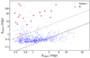 |
Fig. 4. Radio flux density compared to FIR flux density for all sources with a 24 μm counterpart. The red circles indicate the 18 polarised sources with a 24 μm counterpart. The dashed line gives the FRC from Appleton et al. (2004), and the dotted line indicates the radio flux density being ten times greater than for the FRC. |
5.2. Infrared colour-colour diagram
Figure 5 shows the Spitzer MIR colour-colour diagram, where the flux density ratios S8.0 μm/S4.5 μm and S5.8 μm/S3.6 μm are compared with each other. The blue dots represent all our Stokes I sources for which IR counterparts could be found in all four MIR bands. The red circles represent the polarised sources. Following Sajina et al. (2005), who simulated the diagram for a redshift range of 0 < z < 2, region 1 hosts mostly continuum dominated sources at 0 < z < 2 (which is an indication for AGN activity), region 2 selects preferentially poly-aromatic hydrocarbon (PAH) dominated sources at 0.05 < z < 0.3 (which indicates star-forming galaxies), regions 3 and 4 host mainly stellar- and PAH-dominated objects at 0.3 < z < 1.6 and z > 1.6, respectively. For higher redshifts, sources migrate from region 2 to region 4. Therefore, as sources in region 1 can most likely be identified as AGN, all polarised sources in region 1 are classified as AGN. Conversely, the radio emission of the sources in regions 3 and 4 might originate either from AGN activity, while the IR colours are dominated by an old stellar population, or from star formation. However, since we found no polarised source in region 2 (suggesting no certain star-formation contamination), we conclude that there is no evidence of detection of SFGs in polarised emission within our sample. If those were migrated PAH dominated sources from region 2, we would expect to observe at least a few remaining sources at low redshift in region 2 (Hales et al. 2014a). We therefore classified all polarised sources in regions 3 and 4 as AGN. No hint for any detection of SFGs in polarised emission was found in the part of our sample with sufficient multi-wavelength data. We assume this part to be representative for our whole sample. Although this was expected, we note that our classification procedure is just a statistical procedure and does not account for variations within individual sources.
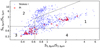 |
Fig. 5. Spitzer MIR colour-colour diagram of the sources in the Lockman Hole field. The blue dots show all sources for which IR counterparts could be found. The open red circles indicate the 34 polarised sources detected in all four IRAC bands. For the explanation of the numbered regions, see Sect. 5. |
5.3. AGN radio power
To differentiate between weaker and stronger AGN we use a criterion from Gendre & Wall (2008) who used the absolute radio luminosity at 1.4 GHz P1400 and the optical B magnitude MB:

We used the optical B magnitude from the catalogue from Tudorica et al. (2017). This cutoff was formerly used as a criterion for a statistical and non-morphological way to classify AGN into FR types (Fanaroff & Riley 1974). Mingo et al. (2019) showed that this criterion does not necessarily hold for the morphological FR types. We thus do not claim our sources to be of the phenotypes FRI or FRII, but differentiate between weaker and stronger radio AGN.
We calculated the absolute radio luminosity in the following way:

where DL is the luminosity distance calculated using the LUMINOSITY_DISTANCE function of the python package astropy.cosmology.FlatLambdaCDM2. We use a Hubble constant  , Ωm = 0.31 and a cosmic microwave background (CMB) temperature of 2.7 K. I is the observed total intensity of our sources, z is the redshift and α the spectral index. Using the redshift information we have for 56 of our sources we classify 14 weaker and 42 stronger AGN (see Fig. 6). The uncertainties shown in Fig. 6 originate from the photometric redshift uncertainties derived from Tudorica et al. (2017), who provide minimum and maximum photometric redshift confidence limits in addition to the maximum posterior point estimate.
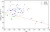 |
Fig. 6. Absolute radio brightness calculated using the photometric redshifts over the B magnitude for the polarised AGN sources. Green symbols represent sources classified as weak AGN and blue ones sources classified as strong AGN. The dashed line is given by Eq. (1) and resembles the cutoff previously used to differentiate between the FR phenotypes. |
6. Results
6.1. Selection effects
An anti-correlation between the fractional polarisation and the total intensity flux density was observed by Tucci et al. (2004), Mesa et al. (2002), and Grant et al. (2010). This anti-correlation was claimed to be caused by either an increasing median redshift of faint sources (Tucci et al. 2004) or a change in the composition of the observed population (Mesa et al. 2002). Hales et al. (2014a) explained this as a selection effect due to incompleteness of the sample, arguing that, for the faintest sources (in total intensity) that reside close to the detection limit of the observations, it is impossible to detect low fractional polarisations.
Figure 7 shows the fractional polarisation as a function of the total intensity for our sources (red), and literature sources from Hales et al. (2014a, blue), Grant et al. (2010, green), and Taylor et al. (2007, magenta). Our sample exceeds the sensitivity of the observations by Tucci et al. (2004), Mesa et al. (2002), Taylor et al. (2007) and Grant et al. (2010) by roughly a factor of six, and is about twice as sensitive as Hales et al. (2014a). We are therefore able to reach lower fractional polarisation levels for sources showing total power emission of the same intensity. The theoretical cutoff under which no sources can be found anymore can simply be described by the sensitivity limit PImin of every sample:

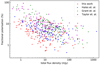 |
Fig. 7. Fractional polarisation over total intensity for sources from different publications. Red triangles pointing to the left represent the sources in this work, blue triangles pointing to the right the ones from Hales et al. (2014a), green stars the ones from Grant et al. (2010), and magenta circles the ones from Taylor et al. (2007). |
For real observations, other effects, such as the reduced sensitivity closer to the borders of the mosaic, reduce this limit and the above equation is only an approximation.
Since we were able to calculate the absolute radio luminosity of 56 sources, we also plotted the fractional polarisation over the absolute radio luminosity in Fig. 8. A physical reason for a correlation between the total flux density and the fractional polarisation should also show up as a correlation between the absolute brightness and the fractional polarisation. Figure 8 does not show explicit hints of such a correlation. This is confirmed by binning the data by their total radio brightness (see Table A.3).
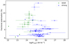 |
Fig. 8. Fractional polarisation over absolute radio brightness for the 56 sources with known photometric redshift. |
We therefore conclude that the observed anti-correlation between fractional polarisation and total intensity has no physical origin and instead, following Hales et al. (2014a), is caused by a selection effect due to limited sensitivity.
6.2. Comparison of different deep fields
We now compare the fractional polarisation of our sources with all available literature data to investigate the dependence of the fractional polarisation on the total power emission (Fig. 9). For this purpose we binned our data by the total intensity of our polarised sources. The bin limits and the respective sizes are listed in Table 1. We have similarly binned the data from Hales et al. (2014a), for the ELAIS-S1 and the CDF-S fields, and from Grant et al. (2010), and included them in Fig. 9 for comparison. We also list the counts per bin for these sources in Table 2. Additional literature data shown in Fig. 9 are taken directly from the publications. The data from Stil et al. (2014) are generated using a stacking technique. With the exception of Stil et al. (2014), Mesa et al. (2002), and Tucci et al. (2004), all publications used in Fig. 9 utilise deep observations of small fields and thus only sample a small part of the sky. An overview of these fields areas and sensitivities is given in Table A.2. For the bright sky, down to fluxes of ∼60 mJy, only NVSS-based data are available in an amount that is usable for statistical comparison. For the fainter sky there are no direct NVSS observations, but instead only the stacked results from Stil et al. (2014). Comparing the small area samples with each other reveals different trends in the median fractional polarisation of the faint polarised radio sky. The sample used here, along with that from Subrahmanyan et al. (2010) and the ELAIS-S1 sample from Hales et al. (2014a), shows an increase in median fractional polarisation to both lower and higher total intensities, around a minimum. On the other hand the median fractional polarisation values of the sample of Rudnick & Owen (2014) and the CDF-S observations by Hales et al. (2014a) increase and finally flatten towards low flux densities. It is important to note, though, that the analysis by Rudnick & Owen (2014) only presents upper limits, which are mainly driven by completeness limitations. However, for the same fluxes the median fractional polarisation of the different fields differs by a factor of two or more. In general, an increase in median fractional polarisation towards low flux densities may be due to the aforementioned completeness limitations. This is, however, in contrast to the observed flattening towards low flux densities. In addition, since all analysis of the faint polarised sky, with the exception of Stil et al. (2014), are based on areas of only several square degrees, sample variance of the underlying large-scale structures (i.e. variation driven by the existence of super-clusters and voids in the fields) are affecting the results. We can therefore conclude that the characteristics of the polarisation properties of the faint sky below 60 mJy are not properly understood and that deeper, wider observations are needed to increase the completeness of these samples.
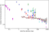 |
Fig. 9. Median fractional polarisation over total intensity for different catalogues. The red dots give the data points of Stil et al. (2014), who used the NVSS catalogue and a stacking technique, and the open turquoise upward (steep) and downward (flat) pointing triangles are the polarised sources from Tucci et al. (2004) of the NVSS split up by a spectral index of −0.5. The open magenta triangles represent the sources from Mesa et al. (2002) split by the same spectral index limit. The magenta circles represent upper limits from the catalogue of Rudnick & Owen (2014). The green stars are from Grant et al. (2010), the green circle from Taylor et al. (2007), and the blue open circles from Subrahmanyan et al. (2010). The triangles pointing to the right are the data from Hales et al. (2014a), the blue ones represent their data for the ELAIS-S1 field, and the turquoise ones their data for the CDF-S field. The red triangles pointing left represent our polarised sample. |
Overview of the bins used for Fig. 9 for the data from Hales et al. (2014b) and Grant et al. (2010).
6.3. Spectral index
Tucci et al. (2004) detected an anti-correlation between the fractional polarisation and the total intensity flux (as already discussed in Sect. 6.1), predominantly for steep spectrum sources (α < −0.5) but only marginally for flat (and inverted) spectrum (α ≥ −0.5) sources. This observation cannot be explained by the selection effect argument of Hales et al. (2014a). Such an effect would affect steep as well as flat spectrum sources. In contrast to the above findings, Mesa et al. (2002) did not find such a strong dependence on the spectral index as Tucci et al. (2004).
Stil & Keller (2015) used stacking to increase the sensitivity and thus fill the gap between our data and the NVSS data. They observe only a weak increasing trend for steep (α < −0.75) and no increase for flat (α > −0.3) spectrum sources, but a strong increasing trend in fractional polarisation for intermediate (−0.75 < α < −0.3) spectrum sources.
In Fig. 10 we show the median fractional polarisation for steep and flat spectrum sources, respectively, as a function of total flux density. The number of sources in each flux bin is given in Table 1.
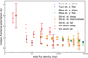 |
Fig. 10. Median fractional polarisation over total intensity for steep and flat spectrum sources for our sample (red) and the ones from Tucci et al. (2004) (blue) and Mesa et al. (2002) (green). Upward pointing triangles represent steep spectrum sources with a spectral index of α ≤ −0.5, and downward pointing triangles represent flat or inverted spectrum sources with a spectral index of α ≥ −0.5. |
The last two bins of the flat spectrum sources need to be excluded from the analysis since they contain a statistically insignificant number of sources: three and one, respectively. It is visible that steep spectrum sources in general have a higher fractional polarisation than flat spectrum sources. Both types scatter in the same way around a constant value of about 3.25% for steep and 1.62% for flat spectrum sources. They show no sign of correlation (nor anti-correlation) between fractional polarisation and total intensity flux density. Only for the bin containing sources with a total flux lower than 4 mJy the fractional polarisation increases rapidly. Since the completeness effect has the strongest influence near the detection limit, this is most likely not caused by physical reasons but rather due to the low completeness in this bin.
We note that the scatter for our sample is intrinsically higher in comparison to the literature values due to the smaller number statistics, when compared to the large samples used for the NVSS analysis.
6.4. Euclidean-normalised polarised differential source counts
In Fig. 11 we present the Euclidean-normalised polarised differential source counts from our sources in the Lockman Hole field. The calculation is based on the code from Herrera Ruiz et al. (2018), which accounts for the higher noise at the mosaic edges. We also accounted for the resolution bias, following the method of Prandoni et al. (2018). The solid black line gives the model for polarised differential component counts given by Hales et al. (2014a), who used the model for total-intensity source counts from Hopkins et al. (2003) and convolved it with a polarised density function fitted to their data. The blue and cyan dots are the data from Hales et al. (2014a) for the CDF-S and the ELAIS-S1 fields. The red triangles represent the polarised differential source counts derived from our sample. For direct comparison, we use the same binning as Hales et al. (2014a) for the CDF-S Field. Following their bin width of 0.16 dex, we extended these bins to lower fluxes, excluding bins with sources that are only detectable in a region of less than 10% of our mosaic. We note that the model from Hales et al. (2014a) was calculated for component rather than source counts, but the authors claim that there is no significant difference between source and component counts for resolutions of 10″ in the millijansky regime and below. However, it is likely that source counts are slightly lower than component counts, especially when comparing different resolutions. The dashed black line gives the differential polarised source counts from O’Sullivan et al. (2008), who used semi-empirical simulations from the European SKA Design Study (SKADS). Using the luminosity they also distinguished between FR I and FR II sources, for which the source counts are given by the green (FR I) and blue (FR II) dashed line. The black dotted line represents their source counts for normal galaxies (NGs) and the dot-dashed line represents the source counts for radio-quiet quasars (RQQs).
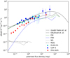 |
Fig. 11. Euclidian-normalised differential source counts at 1.4 GHz in polarised intensity from our Lockman Hole observations (red triangles). Component counts from Hales et al. (2014a) for CDF-S (blue) and ELAIS-S1 (turquoise) are given for comparison. The solid black line shows the model prediction from Hales et al. (2014a). The other lines are from the simulations of O’Sullivan et al. (2008); the dashed black line gives the total polarised differential source counts, the dashed green line gives the FR I source counts, and the blue one gives the FR II source counts. The black dotted line represents the NGs, and the dot-dashed black line the RQQs. |
With our study we confirm the decreasing trend for fainter source number counts, while also finding an offset (of up to a factor of three) towards smaller number counts, over the whole flux range, when comparing our data to those of Hales et al. (2014a). We note, though, that our source counts at low flux densities show a similar trend compared to the FR II source counts from O’Sullivan et al. (2008), even though they are higher. Several different reasons can possibly explain this behaviour. First of all, we note that a small offset to the model from Hales et al. (2014a) was expected since we used their fractional polarisation distribution function, which might not properly represent the distribution of our data and component counts might deliver slightly higher values than source counts. In addition, sample variance introduced by large cosmological structures like super-clusters and voids influence the composition of the source counts significantly for surveys spanning only modest (i.e. a few square degrees) areas on-sky. We expand on the relevance of sample variance in Sect. 8. The lower source counts compared to the simulations of O’Sullivan et al. (2008) and Hales et al. (2014a) mean that we find a dearth of faint sources in our sample. This is discussed further in Sect. 8.3.
6.5. Redshift and fractional polarisation
We used the photometric redshift information we have for 56 of our sources to compare the redshift with the fractional polarisation. To this end we binned our sources over five redshift ranges the corresponding numbers are given in Table 3.
In Fig. 12 we show the median fractional polarisation as a function of redshift. The given uncertainties are calculated assuming Poisson statistics. We find a decrease in median fractional polarisation towards higher redshift ranges.
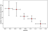 |
Fig. 12. Median fractional polarisation over redshift. The error bars of the median fractional polarisation are the Poisson errors, whereas the error bars in the x direction give the bin width. |
An anti-correlating trend was already found by Hammond et al. (2012) for an NVSS polarised sample. They explained it to be due to different types of sources being dominantly observed at different redshifts. Where their low-redshift sources are mostly lobes of galaxies with a high median fractional polarisation they found core dominated quasars with a low fractional polarisation at higher redshifts. They found no such trend for either type only. In contrast to our study they found a strong decrease in fractional polarisation and then a flattening. Since we do not have such a clear turnoff, but a decrease over the full sampled redshift range, and no other hint for different source types dominating different redshift ranges, this cannot be the reason for our observed anti-correlation. We note that, in contrast to our study, Hammond et al. (2012) observed the bright polarised sky with a beam that was about three times larger than our beam.
We first investigate whether we find selection effects in our data, such as those discussed in Sect. 6.1. For this effect, in order to explain the anti-correlation between fractional polarisation and redshift, a correlation between redshift and observed total flux density would be necessary. Therefore, the observed flux would need to increase with increasing redshift. We find no such correlation, and thus cannot explain the anti-correlation between fractional polarisation and redshift as being due to selection effects.
It is known that the different FR phenotypes also show different polarisation behaviour. FR I objects show on average a higher integrated fractional polarisation compared to FR II sources (the latter generally exhibit 4% polarisation; Saikia & Salter 1988). Additionally, FR II sources are usually more luminous than FR I sources. These two effects can easily cause a bias towards one or the other FR type, for the high or low-redshift bins. Even though we are not able to investigate this bias, we want to filter our statistics by differentiating between weak and strong sources (see Sect. 5.3) to investigate the effect of the brightness of the sources on the observed anti-correlation.
Figure 13 shows the absolute radio brightness of our 56 polarised sources used in this analysis as a function of their photometric redshift. With increasing redshift we observed fewer faint and more bright sources. Since the brightest radio sources are (in general) quite rare, it is more likely to observe them with increasing volume (and thus with increasing redshift Ledlow & Owen 1996). The loss of faint sources at high redshift can be explained by selection bias, as fainter sources at high redshift will naturally fall below our detection limit.
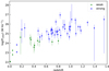 |
Fig. 13. Absolute radio brightness calculated using the photometric redshifts over the redshift. The errors take only the uncertainties of the photometric redshifts into account. |
Figure 13 shows that our sample is dominated by weak sources for low z and by strong sources for high z. The last two bins in Fig. 12 are free of any influence from weak sources. We therefore conclude that the increase in bright sources with redshift cannot alone induce the anti-correlation between fractional polarisation and redshift, given our demonstration (in Fig. 8) that there is no correlation between fractional polarisation and absolute radio brightness for our sources.
In Fig. 14 we again show the median fractional polarisation over a given redshift range, separated into weak and strong sources. The bins are chosen using the same limits as previously with steps of Δz = 0.3 for the first four bins and Δz = 0.4 for the last bin (see Table 3).
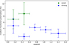 |
Fig. 14. Median fractional polarisation over redshift for weak and strong sources. We excluded those bins containing fewer than three sources. In particular, this affects the third bin of weak sources. The error bars of the median fractional polarisation are the Poisson errors, whereas the error bars in redshift give the bin size. |
Since the whole sample contains only 56 sources, it is worth noting that the number of sources in individual bins is small. Only the first two bins of weak sources contain a statistically significant number of sources, so we opted to exclude the later bins from our subsequent analysis.
The weak low-redshift sources show an increase in median fractional polarisation with increasing redshift. We note that only 12 sources contribute to this statistic within two bins, so that the significance is limited. The strong sources show a decreasing trend of fractional polarisation over the whole redshift range. Only the second bin shows a rapid drop. Since only three sources contribute to this bin, we assume it to be an outlier and not of statistical significance.
7. Influence of cosmic evolution
The observed anti-correlation between median fractional polarisation and redshift (Sect. 6.5) can have several origins, each of which we discuss individually in this section.
First, we want to consider the depolarisation of the emission by turbulent magnetic cells, the effect known as Faraday dispersion. The ratio DP between the initial polarised flux and the observed polarised flux is strongly wavelength dependent. We also must distinguish between two distinct forms of Faraday dispersion: the external Faraday dispersion (EFD) and the internal Faraday dispersion (IFD) cases (Sokoloff et al. 1998). For AGN sources, Faraday dispersion is dominated by external fields situated between the emitting source and the observer. In this case the depolarisation can be calculated by:
For both cases, σ is the same and is defined as:

where ⟨ne⟩ is the average electron density in cm−3, ⟨Bturb⟩ is the average turbulent magnetic field strength in μG, d is the turbulent cell size in pc, L is the path-length in pc, and f is the filling factor of the turbulent cells causing the depolarisation.
7.1. Redshift-depolarisation dependence
Due to the cosmologically significant redshift range we are probing in this analysis, we first explore the effect of differing initial wavelengths. Sources at high redshift, detected in our sample at λ20 cm, emit their actual emission at significantly shorter wavelengths. We can calculate the emitted wavelength λi in the source’s rest-frame for our sample using the standard equation:

where λobs is the observed wavelength and z is the redshift. For our sample, the emission we receive for sources at z = 1.4 would originally be emitted at a wavelength of λ ≈ 8 cm.
Since we assume all our sources to be AGN, this shift of wavelength should not have an effect on the initial fractional polarisation. Anyhow, Conway et al. (1977) showed a fractional polarisation of 4% at 21 cm and of 6% at 6 cm for a sample of mainly nearby AGN. We attribute this to physical depolarisation effects.
The shorter wavelength are less affected by IFD and EFD (see Eq. (4)) than the longer wavelengths. This is in contrast to our observed trend, where the higher-redshift sources (emitting at a shorter wavelength) are observed to be less polarised than the lower redshift, longer initial wavelength sources.
Therefore, we conclude that we must account for the different initial wavelengths of emission (due to the location of the sources at different redshifts) and the influence this has on depolarisation.
7.2. Morphology and source environment
We now assume the morphology and environments of sources change as a function of redshift, due to the evolution of cosmic structures over time. The high redshift sources for which the observed anticorrelation is stronger are mostly identified as strong AGN. We assume them to be mostly FR II sources and thus members of galaxy groups (Ledlow & Owen 1996). These galaxy groups were less relaxed in the earlier stages of the Universe (Noble et al. 2017), which can influence their magnetic field strengths and morphologies (and therefore their intrinsic polarisation characteristics). That these sources have such a high radio luminosity hints at them being jet dominated. In combination with the less relaxed clusters, this might cause a stronger impact of the Laing-Garrington effect (Garrington et al. 1988), which leads to a higher depolarisation of the jet further away from the observer. Thus, for average polarisation values of these sources, we would only be able to detect a smaller fraction of the polarised emission.
For extended sources we also have to account for beam depolarisation since the projected angular size of sources decrease with increasing redshift up to z ≈ 0.5. For higher redshifts the projected angular size stays nearly constant with increasing redshift (Middelberg et al. 2011) up to a value of z = 1.5, where it turns around. We do not have sources beyond this limit in our sample. So that the decrease in fractional polarisation for redshifts of z > 0.6 shown in Fig. 14 cannot be explained by this effect.
7.3. External Faraday dispersion
In the previous subsection we considered the sources’ direct environment as the primary cause of depolarisation. We now want to consider the medium along the line of sight as a possible origin of the observed trend. Polarised emission of sources further away cross a larger volume of magneto-ionic medium. This increases the chance for the (initially polarised) emission to encounter turbulent magnetic cells in intergalactic space along the line of sight, which induce depolarisation due to EFD. In this case σ is no longer a constant for all sources, as the path length L is dependent on the redshift. Anyhow, this increasing L does not have a significant effect on the EFD if we assume ⟨Btubr⟩ = 0.037 μG (Vernstrom et al. 2019) being the turbulent magnetic field strength over the whole line of sight.
We therefore conclude that external Faraday dispersion induced by a turbulent intergalactic magnetic field cannot explain the observed anti-correlation found, assuming a constant electron density and a constant magnetic field strength.
This is in agreement with previous works that assume the electron density as well as the magnetic fields strength to be dependent on z. For a cosmological significant redshift, however, we cannot assume ne and B to be constant: rather we expect to find ne ∝ (1 + z)3 (O’Sullivan et al. 2020; Blasi et al. 1999; Pshirkov et al. 2016). This increase in the electron density might also lead to an increase in the magnetic field strength as a function of redshift: B(z) = B0[ne(z)/n0(z)] (O’Sullivan et al. 2020). It is also unlikely that, for an increasing magnetic field strength, the turbulence remains constant. This implies that we must also assume a possibly redshift dependent ⟨Bturb⟩. An increase in ⟨ne⟩ and ⟨Bturb⟩ with redshift may induce a higher depolarisation for more distant sources, and thus explain the anti-correlation found between fractional polarisation and redshift. However, this also means that L, λ, ⟨ne⟩, and ⟨Bturb⟩ are all interconnected and redshift dependent. An exploration of these effects, though, would require an extension of Eqs. (4) and (5); this is naturally a considerable task, and we leave such an investigation to future works.
8. Discussion
8.1. Observations of the faint polarised sky
In Sect. 6.2 we showed that the different deep field samples show different behaviours of fractional polarisation towards fainter polarised fluxes. One could argue that these different trends were caused by one or more of: instrumental effects, differences in the telescopes used, different software, and differences in data reduction strategies. Countering these possibilities, however, are the two fields analysed by Hales et al. (2014a), which still show a difference in their trends between each other. These observations were conducted using the same telescope array, software, and reduction strategies, suggesting that other explanations for these polarisation effects should be considered.
Nearly all presented analyses are observations of survey areas spanning up to 15 deg2, meaning that differences can be caused by sample variance: inhomogeneities in the source distribution on-sky caused by differences in large-scale structures within a small field. In addition to this, the observed fields on-sky are not randomly selected, but rather are selected specifically due to some special characteristic: the Lockman Hole, for example, shows the lowest HI column density over the entire sky (Lockman et al. 1986). Sources observed in this field are known to have a systematically high median redshift compared to other fields of equivalent depth (z ∼ 0.99 in Luchsinger et al. 2015, which is similar to our sample’s median redshift of z ∼ 0.75). The ELAIS fields are selected because of their low 100 μm intensity and their high galactic latitude (Oliver et al. 2000). The CDF-S has like the Lockman Hole a low HI column density (Giacconi et al. 1999). All of these preferential field selections may introduce biases in the detected source distributions for these fields, when compared to a statistically ‘normal’ patch of sky of equivalent area.
8.2. Spectral index - Fractional polarisation dependence
In Sect. 6.3 we compared the fractional polarisation of steep and flat spectrum sources depending on their total intensity. In contrast to Tucci et al. (2004), but in agreement with Mesa et al. (2002), we find no difference in the correlation between spectral index and fractional polarisation for steep and flat spectrum sources. In agreement with Stil & Keller (2015), steep spectrum sources in our sample are, however, generally more polarised than flat spectrum sources; this difference was not observed by Mesa et al. (2002) nor Tucci et al. (2004). It is worth noting, though, that both of these previous studies used the spectral index measured between 1.4 GHz and 5 GHz, whereas we use the spectral index measured between 1.4 GHz and 150 MHz and Stil & Keller (2015) use the spectral index measured between 1.4 GHz and 325 MHz. At these low frequencies we must account for additional absorption effects like synchrotron self-absorption and thermal absorption, which lead to lower measured 150 MHz fluxes and thus a flattening of the spectral index (compared to the spectral indices measured at higher frequencies). As a result, some of our flat spectrum sources might indeed be defined as steep spectrum sources at higher frequencies. This might decrease the difference in fractional polarisation between steep and flat spectrum sources, and reconcile the difference found between our results and those of Mesa et al. (2002), Tucci et al. (2004). This explanation is also supported by the fact that Stil & Keller (2015) also observe a higher fractional polarisation for steep spectrum sources than for flat spectrum sources and they use the spectral index towards the MHz-regime.
It should also be recognised that we are observing the faint polarised radio-sky, while Tucci et al. (2004) and Mesa et al. (2002) are working with the bright polarised radio-sky. Stil & Keller (2015) are probing the range in between, due to their stacking technique. Even in the bright regime they observe a strong difference between steep and flat spectrum sources. Therefore, we conclude that the different wavelengths used for the derivation of the spectral indices are causing the different observed median fractional polarisation for steep and flat spectrum sources. Due to this we can neither confirm nor contradict the different trends for steep and flat spectrum sources observed by Tucci et al. (2004) with our observation.
8.3. Source counts
In Sect. 6.4 we presented the differential Euclidean-normalised polarised source counts of our field, compared to the observations from Hales et al. (2014a) and the simulations from O’Sullivan et al. (2008). To low flux densities we observed lower source counts than expected from both previous observations and the models. Since we observe sources with a high median redshift z = 0.75 than previous studies, this difference may be driven by a dearth of faint near sources in the Lockman Hole field. Figure 15 shows the same plot as given in Fig. 11 but with two additional lines. We used the simulations from O’Sullivan et al. (2008), for the individual source types, to find a fit for our observations. The simulations are based on complex functions that we do not want to replicate here, so we are not fitting our data directly. Using the summation of the individual source counts as a1 ⋅ FR I + a2 ⋅ FR II we end up with the green dotted line using a1 = 0.21 and a2 = 1. That is, we assume that we observe only 21% of the FR I sources compared to O’Sullivan et al. (2008). Since our sample is dominated by bright sources, we ignore the contribution from NG or RQQ. The FR sample from O’Sullivan et al. (2008) goes down to flux densities of about 1 mJy and contains ∼99.88% FR I sources. As discussed in Sect. 5.3, we cannot classify our sources following the FR classification, but our cutoff for weaker and stronger AGN was previously used for this purpose (Gendre & Wall 2008). We only find ∼21.43% of the 56 sources that we were able to classify to be weak, and thus likely FRI. We assume those 56 sources to be representative for our whole sample, suggesting that we are biased towards lower FR I source numbers. We note that the simulations from O’Sullivan et al. (2008) are based on simulations from Wilman et al. (2008) and thus extrapolated from the observed source distributions at 151 MHz, leading to another unknown parameter for our analysis.
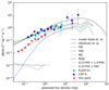 |
Fig. 15. Similar to Fig. 11, giving the Euclidian-normalised differential source counts. The additional curves are defined by the summation of the source counts from O’Sullivan et al. (2008), a1 ⋅ FR I + a2 ⋅ FR II, where for the green dotted line a1 = 0.21 and a2 = 1 and for the blue dotted line a1 = 0.21 and a2 = 1.5. |
The source density observed by Hales et al. (2014a) is between 16 and 23 sources per deg2, with a central RMS of 25 μJy beam−1. We observed 23 polarised sources per deg2 with a lower central RMS of 7 μJy beam−1. The differences in source density between the different fields from Hales et al. (2014a), as well as the possible dearth of FR I sources in our observations, can originate from the already discussed differences in source characteristics of different deep fields (see Sects. 6.2 and 8.1). This difference might also explain a slight difference we have between our source density and the density predicted by Rudnick & Owen (2014) from their deep GOODS-N observations of 35 ± 10 sources per deg2 for a flux regime of about 50 μJy, which is in good agreement with our flux regime, taking into account our detection threshold of 6.25σ.
In Fig. 16 we show the redshift distribution of the 56 sources for which we are able to determine redshifts. In agreement with previous observations of the Lockman Hole (e.g., Luchsinger et al. 2015; Fotopoulou et al. 2012) we observe a dearth of low-redshift sources, up to a redshift of z ∼ 0.4. In Fig. 3 of Luchsinger et al. (2015) a lack of low-z sources is visible, compared to the simulations from Wilman et al. (2008). Luchsinger et al. (2015) explained this as being due to the over-resolution of low-z sources, so the emission from near sources is resolved out. If this were true, a lower-resolution survey of the field should recover this population of low-redshift sources. The resolution of our PI and total intensity map is 15″, while the resolution of Luchsinger et al. (2015) is 4″. Nonetheless, we recover the same source redshift distribution as Luchsinger et al. (2015). We therefore conclude that this dearth of low-redshift sources compared to the simulation of Wilman et al. (2008) is not due to them being over-resolved and lost from the imaging. Further, the observations of Fotopoulou et al. (2012) show the same redshift distribution for X-ray sources and normal optical galaxies. It is thus possible that the difference between the Lockman Hole observations and the simulations of Wilman et al. (2008) and the observations of Hales et al. (2014b) are driven by a combination of large-scale structure variations (i.e. sample variance), which at our estimated distances of up to z ≈ 1.4 can fill an entire field of the size of the Lockman Hole, and by differences in source properties between small survey areas. Finally, FR I sources dominate the observations at low redshift (Ledlow & Owen 1996). We can therefore conclude that a possible explanation of the low source counts at low flux densities is a dearth of low-redshift FR I sources.
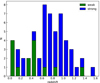 |
Fig. 16. Histogram of the photometric redshifts of the 56 sources classified as weak and strong sources. |
So far we have only taken low flux densities into account in our discussion. To also account for the higher flux densities, we adjusted the relative values of a1 and a2 to approximately represent our data. Values of a1 = 0.21 and a2 = 1.5 were used to generate the blue dotted line in Fig. 15. Since we cannot fit the values to our data, these values are only rough estimates; they are designed only to that a higher fraction of FR II sources (i.e. a2 = 1.5) explains higher source counts at high fluxes, while the low fraction of FR I sources (i.e. a1 = 0.21) still dominates the low source counts at low fluxes, shown by the green dotted line in Fig. 15. We note that we therefore cannot exclude other combinations of a1 and a2 to give similar results.
A higher fraction of FR II sources could be due to a large-scale overdensity of sources at high redshift. This is indicated by the distributions from Luchsinger et al. (2015) (Fig. 3) and Fotopoulou et al. (2012) (Figs. 11 and 15), which show peaks at z ≈ 0.6 and z ≈ 1.5. Henry et al. (2014) also suggest that such an over-dense structure is present in the Lockman Hole at z = 1.71, which could also contribute to our observations. Due to the lack of faint sources it might be necessary to distinguish between the bright sources, where our source counts fit the simulations of O’Sullivan et al. (2008), and faint sources, where the loss of FR I sources becomes dominant.
Including NG and RQQ in our fit leads to a flattening of the source counts at around 10−1 mJy, which would cause a stronger effect than that which is observed in our data. This again fits to our previous assumption: that all detected polarised sources can be classified as AGN.
For a direct comparison of polarised sources redshift distribution, we compared the redshift distribution of our sample to the simulated AGN sample from Bonaldi et al. (2019). To have an estimate on the effect of local variations in small fields compared to larger ones, we plot the distribution of the deep simulation as well as of the medium simulation from Bonaldi et al. (2019). For comparability, we set a cutoff of 6.25 times our central RMS on the simulated data, to only include sources that would be detectable in our observation. Figure 17 shows the normalised histogram of our sources and both samples from Bonaldi et al. (2019). For low redshifts we detected more sources than expected by the simulation, while we have a loss of high redshift sources. Apparently faint sources can either be nearby with low intrinsic (absolute) brightnesses or be luminous sources located at high redshift. The loss of faint low-z sources was discussed previously, in the context of the loss of near FR I sources. Figure 17 hints at a loss of apparently faint sources at high redshift, as another possible reason for our observed source counts. However, the comparison of the deep and the medium simulation of Bonaldi et al. (2019) shows that, even for the same simulation, there is significant variations caused by the survey area and volume. This confirms our conclusion that different fields covering only several square degrees are showing differences in source count statistics of several orders. This is again in good agreement with our observed differences in the source properties of different, small area fields (see Sects. 6.2 and 8.1).
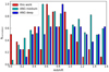 |
Fig. 17. Normed histogram of the photometric redshift of our 56 polarised sources (red), compared to the deep (blue) and medium (cyan) simulations of Bonaldi et al. (2019), where we used a cutoff of 6.25 times our central RMS. We only include sources with flux densities comparable to those of our sample. We also normed the maximum of each sample to 1 in the histogram to allow different sample sizes to be compared with one another. |
8.4. Impact of cosmic evolution
In Sect. 7 we discussed several possible reasons for our observed anti-correlation between fractional polarisation and redshift. It is most likely that the origin of this trend can be found in the evolution and structure of the Universe. It might be that the sources themselves are intrinsically different at different redshifts, due to the evolution of environment with redshift, which also causes different depolarisation effects. Finally, there are also hints (O’Sullivan et al. 2020; Blasi et al. 1999; Pshirkov et al. 2016) that not only the environment but the cosmic magnetic field changes with an evolving Universe.
9. Summary
We present a new deep-field analysis of polarised sources in the Lockman Hole at 1.4 GHz, using a bespoke polarised mosaic with a central RMS of 7 μJy beam−1. We find 150 polarised sources in an area of 6.5 deg2 out of 1708 total-intensity sources in this field (8.8%). This equates to a polarised source density of 23/deg2.
We were able to explore fainter polarised flux densities than previous studies with comparable areas. All our sources were classified as AGN. This result is in agreement with the findings from Hales et al. (2014a).
We found mainly faint polarised sources with only a few percent polarisation; the mean fractional polarisation is 5.4%. The highest fractional polarisation found is ∼21%.
A direct morphological classification, following the FR classification scheme, was not possible for the majority of our sources in the sample, as most sources are unresolved. Using the absolute radio brightness and the optical B magnitude as a classification criterion, which was previously used for classifying according to the FR classification, we were able to classify 14 sources as weak and 42 sources as strong sources.
When comparing our catalogue to other deep field catalogues from previous work, we found significant differences in median fractional polarisation as a function of total intensity, both between our dataset and previous work and between individual previous studies. We attribute these differences to sample variance caused by large-scale structures within different small on-sky areas that causes different source populations to be observed within the various fields.
We present Euclidean-normalised differential source counts for our field. A comparison to the analysis of previous publications shows hints that our sample is dominated by FR II sources, while most other studies are dominated by FR I sources. We found hints for a dearth of low-redshift sources in the Lockman Hole field, taking into account observations at other wavelengths. This is again in agreement with previous work, which has shown that the Lockman Hole is under-dense at low redshift (Luchsinger et al. 2015; Fotopoulou et al. 2012).
We were able to cross-identify 56 of our sources with a deep optical catalogue containing photometric redshift information. Using this redshift information, we found an anti-correlation between median fractional polarisation and redshift. This trend is visible for the whole sample. Strong sources alone show the same behaviour, while the same trend is not visible for weak sources. We discuss several possible explanations for this anti-correlation. We conclude that this trend originates in host sources being contained within different environments as a function of redshift and/or in a significant evolution of the cosmic magnetic field (in both field strength and morphology) over the lifetime of the Universe.
Acknowledgments
The research at AIRUB is supported through BMBF project grants D-LOFAR IV (FKZ: 05A17PC1) and D-MeerKAT (FKZ: 05A17PC2). A. H. W. is supported by an European Research Council Consolidator Grant (No. 770935). IP acknowledges support from INAF under the SKA/CTA PRIN “FORECaST” and the PRIN MAIN STREAM “SAuROS” projects. We want to thank J. M. Stil for providing the data from his publication.
References
- Abolfathi, B., Aguado, D. S., Aguilar, G., et al. 2018, ApJS, 235, 42 [NASA ADS] [CrossRef] [Google Scholar]
- Adebahr, B., Krause, M., Klein, U., et al. 2013, A&A, 555, A23 [NASA ADS] [CrossRef] [EDP Sciences] [Google Scholar]
- Appleton, P. N., Fadda, D. T., Marleau, F. R., et al. 2004, ApJS, 154, 147 [NASA ADS] [CrossRef] [Google Scholar]
- Beck, R. 2015, A&ARv, 24, 4 [Google Scholar]
- Blandford, R., Meier, D., & Readhead, A. 2019, ARA&A, 57, 467 [NASA ADS] [CrossRef] [Google Scholar]
- Blasi, P., Burles, S., & Olinto, A. V. 1999, ApJ, 514, L79 [NASA ADS] [CrossRef] [Google Scholar]
- Bonaldi, A., Bonato, M., Galluzzi, V., et al. 2019, MNRAS, 482, 2 [NASA ADS] [CrossRef] [Google Scholar]
- Boyle, B. J., & Terlevich, R. J. 1998, MNRAS, 293, L49 [CrossRef] [Google Scholar]
- Brentjens, M. A., & de Bruyn, A. G. 2005, A&A, 441, 1217 [NASA ADS] [CrossRef] [EDP Sciences] [Google Scholar]
- Condon, J. J., Cotton, W. D., Greisen, E. W., et al. 1998, AJ, 115, 1693 [NASA ADS] [CrossRef] [Google Scholar]
- Conway, R. G., Burn, B. J., & Vallée, J. P. 1977, A&AS, 27, 155 [NASA ADS] [Google Scholar]
- Fanaroff, B. L., & Riley, J. M. 1974, MNRAS, 167, 31P [Google Scholar]
- Farnes, J. S., Gaensler, B. M., & Carretti, E. 2014, ApJS, 212, 15 [NASA ADS] [CrossRef] [Google Scholar]
- Fazio, G. G., Hora, J. L., Allen, L. E., et al. 2004, ApJS, 154, 10 [NASA ADS] [CrossRef] [Google Scholar]
- Fiore, F., Puccetti, S., Grazian, A., et al. 2012, A&A, 537, A16 [NASA ADS] [CrossRef] [EDP Sciences] [Google Scholar]
- Fotopoulou, S., Salvato, M., Hasinger, G., et al. 2012, ApJS, 198, 1 [NASA ADS] [CrossRef] [Google Scholar]
- Garrington, S. T., Leahy, J. P., Conway, R. G., & Laing, R. A. 1988, Nature, 331, 147 [NASA ADS] [CrossRef] [Google Scholar]
- Gendre, M. A., & Wall, J. V. 2008, MNRAS, 390, 819 [NASA ADS] [Google Scholar]
- Giacconi, R., Rosati, P., Norman, C., et al. 1999, in Highlights in X-ray Astronomy, eds. B. Aschenbach, M. J. Freyberg, et al., 272, 419 [NASA ADS] [Google Scholar]
- Grant, J. K., Taylor, A. R., Stil, J. M., et al. 2010, ApJ, 714, 1689 [NASA ADS] [CrossRef] [Google Scholar]
- Greisen, E. W. in Acquisition, Processing and Archiving of Astronomical Images, 125 [Google Scholar]
- Hales, C. A., Norris, R. P., Gaensler, B. M., & Middelberg, E. 2014a, MNRAS, 440, 3113 [NASA ADS] [CrossRef] [Google Scholar]
- Hales, C. A., Norris, R. P., Gaensler, B. M., et al. 2014b, MNRAS, 441, 2555 [NASA ADS] [CrossRef] [Google Scholar]
- Hammond, A. M., Robishaw, T., & Gaensler, B. M. 2012, ArXiv e-prints [arXiv:1209.1438] [Google Scholar]
- Helfand, D. J., White, R. L., & Becker, R. H. 2015, VizieR Online Data Catalog, VIII/92 [Google Scholar]
- Henry, J. P., Aoki, K., Finoguenov, A., et al. 2014, ApJ, 780, 58 [Google Scholar]
- Herrera Ruiz, N., Middelberg, E., Deller, A., et al. 2018, A&A, 616, A128 [EDP Sciences] [Google Scholar]
- Hopkins, A. M., Afonso, J., Chan, B., et al. 2003, AJ, 125, 465 [NASA ADS] [CrossRef] [Google Scholar]
- Lamee, M., Rudnick, L., Farnes, J. S., et al. 2016, ApJ, 829, 5 [NASA ADS] [CrossRef] [Google Scholar]
- Ledlow, M. J., & Owen, F. N. 1996, AJ, 112, 9 [Google Scholar]
- Lockman, F. J., Jahoda, K., & McCammon, D. 1986, ApJ, 302, 432 [NASA ADS] [CrossRef] [Google Scholar]
- Lonsdale, C. J., Smith, H. E., Rowan-Robinson, M., et al. 2003, PASP, 115, 897 [NASA ADS] [CrossRef] [Google Scholar]
- Luchsinger, K. M., Lacy, M., Jones, K. M., et al. 2015, AJ, 150, 87 [CrossRef] [Google Scholar]
- Mahony, E. K., Morganti, R., Prandoni, I., et al. 2016, MNRAS, 463, 2997 [NASA ADS] [CrossRef] [Google Scholar]
- Martin, D. C., Fanson, J., Schiminovich, D., et al. 2005, ApJ, 619, L1 [Google Scholar]
- McMullin, J. P., Waters, B., Schiebel, D., Young, W., & Golap, K. 2007, in Astronomical Data Analysis Software and Systems XVI, eds. R. A. Shaw, F. Hill, & D. J. Bell, ASP Conf. Ser., 376, 127 [Google Scholar]
- Mesa, D., Baccigalupi, C., De Zotti, G., et al. 2002, A&A, 396, 463 [NASA ADS] [CrossRef] [EDP Sciences] [Google Scholar]
- Middelberg, E., Norris, R. P., Hales, C. A., et al. 2011, A&A, 526, A8 [NASA ADS] [CrossRef] [EDP Sciences] [Google Scholar]
- Mignano, A., Prandoni, I., Gregorini, L., et al. 2008, A&A, 477, 459 [NASA ADS] [CrossRef] [EDP Sciences] [Google Scholar]
- Mingo, B., Croston, J. H., Hardcastle, M. J., et al. 2019, MNRAS, 488, 2701 [NASA ADS] [CrossRef] [Google Scholar]
- Mohan, N., & Rafferty, D. 2015, PyBDSF: Python Blob Detection and Source Finder [Google Scholar]
- Noble, A. G., McDonald, M., Muzzin, A., et al. 2017, ApJ, 842, L21 [Google Scholar]
- Offringa, A. R., de Bruyn, A. G., Biehl, M., et al. 2010, MNRAS, 405, 155 [NASA ADS] [Google Scholar]
- Oliver, S., Rowan-Robinson, M., Alexander, D. M., et al. 2000, MNRAS, 316, 749 [NASA ADS] [CrossRef] [Google Scholar]
- Oliver, S. J., Bock, J., Altieri, B., et al. 2012, MNRAS, 424, 1614 [NASA ADS] [CrossRef] [EDP Sciences] [Google Scholar]
- O’Sullivan, S., Stil, J., Taylor, A. R., et al. 2008, in The role of VLBI in the Golden Age for Radio Astronomy, 9, 107 [Google Scholar]
- O’Sullivan, S. P., Brüggen, M., Vazza, F., et al. 2020, MNRAS, 495, 2607 [NASA ADS] [CrossRef] [Google Scholar]
- Perley, R. A., & Butler, B. J. 2017, ApJS, 230, 7 [NASA ADS] [CrossRef] [Google Scholar]
- Prandoni, I., Guglielmino, G., Morganti, R., et al. 2018, MNRAS, 481, 4548 [NASA ADS] [CrossRef] [Google Scholar]
- Pshirkov, M. S., Tinyakov, P. G., & Urban, F. R. 2016, Phys. Rev. Lett., 116, 191302 [NASA ADS] [CrossRef] [PubMed] [Google Scholar]
- Rieke, G. H., Young, E. T., Engelbracht, C. W., et al. 2004, ApJS, 154, 25 [NASA ADS] [CrossRef] [Google Scholar]
- Rudnick, L., & Owen, F. N. 2014, ApJ, 785, 45 [NASA ADS] [CrossRef] [Google Scholar]
- Saikia, D. J., & Salter, C. J. 1988, ARA&A, 26, 93 [NASA ADS] [CrossRef] [Google Scholar]
- Sajina, A., Lacy, M., & Scott, D. 2005, ApJ, 621, 256 [NASA ADS] [CrossRef] [Google Scholar]
- Sault, R. J., Teuben, P. J., & Wright, M. C. H. 1995, in Astronomical Data Analysis Software and Systems IV, eds. R. A. Shaw, H. E. Payne, & J. J. E. Hayes, ASP Conf. Ser., 77, 433 [Google Scholar]
- Sokoloff, D. D., Bykov, A. A., Shukurov, A., et al. 1998, MNRAS, 299, 189 [NASA ADS] [CrossRef] [Google Scholar]
- Stil, J., & Keller, B. 2015, in Advancing Astrophysics with the Square Kilometre Array (AASKA14), 112 [Google Scholar]
- Stil, J. M., Keller, B. W., George, S. J., & Taylor, A. R. 2014, ApJ, 787, 99 [NASA ADS] [CrossRef] [Google Scholar]
- Subrahmanyan, R., Ekers, R. D., Saripalli, L., & Sadler, E. M. 2010, MNRAS, 402, 2792 [NASA ADS] [CrossRef] [Google Scholar]
- Taniguchi, Y. 2004, Prog. Theor. Phys. Suppl., 155, 202 [Google Scholar]
- Taylor, A. R., Stil, J. M., Grant, J. K., et al. 2007, ApJ, 666, 201 [NASA ADS] [CrossRef] [Google Scholar]
- Tucci, M., Martínez-González, E., Toffolatti, L., González-Nuevo, J., & De Zotti, G. 2004, MNRAS, 349, 1267 [NASA ADS] [CrossRef] [Google Scholar]
- Tudorica, A., Hildebrandt, H., Tewes, M., et al. 2017, A&A, 608, A141 [NASA ADS] [CrossRef] [EDP Sciences] [Google Scholar]
- Vernstrom, T., Gaensler, B. M., Vacca, V., et al. 2018, MNRAS, 475, 1736 [NASA ADS] [CrossRef] [Google Scholar]
- Vernstrom, T., Gaensler, B. M., Rudnick, L., & Andernach, H. 2019, ApJ, 878, 92 [NASA ADS] [CrossRef] [Google Scholar]
- Wall, J. V. 1998, in Cosmological Inference from New Radio Surveys, eds. M. N. Bremer, N. Jackson, & I. Perez-Fournon, Astrophys. Space Sci. Lib., 226, 129 [NASA ADS] [Google Scholar]
- Wall, J. V., Jackson, C. A., Shaver, P. A., Hook, I. M., & Kellermann, K. I. 2005, A&A, 434, 133 [NASA ADS] [CrossRef] [EDP Sciences] [Google Scholar]
- Werner, M. W., Roellig, T. L., Low, F. J., et al. 2004, ApJS, 154, 1 [NASA ADS] [CrossRef] [Google Scholar]
- Wilman, R. J., Miller, L., Jarvis, M. J., et al. 2008, MNRAS, 388, 1335 [NASA ADS] [Google Scholar]
Appendix A: Additional tables
Pointing centres.
Overview of deep field observations from the literature.
Total radio brightness bins, numbers, and median fractional polarisation for the 56 sources with known photometric redshift.
Euclidean-normalised polarised differential source counts from Fig. 11.
Table A.5 is a short example of our catalogue. The columns are as follows.
-
Column 1 Source name and number; additional letters (A, B, etc.) indicate the individual components of one specific source.
-
Columns 2, 3, 4, and 5 1.4 GHz position of the polarised source with their uncertainties.
-
Columns 6 and 7 Integrated polarised flux density and its uncertainty.
-
Columns 8 and 9 Integrated total flux density and its uncertainty (only given for sources, not for individual components).
-
Columns 10 and 11 Fractional polarisation and its uncertainty.
-
Column 12 S-Code from pyBDSF; for components and single-component sources: ‘S’: the source is a single-Gaussian source, ‘M’: a multi-Gaussian source, ‘G’ a single-Gaussian component in a multi component source; For multi component sources: ‘Sum’ for sources identified by pyBDSF, ‘Com’ for sources identified by visual inspection and/or comparison with other wavelength. The components of sources identified by hand, have the code ‘Com’ attached.
-
Column 13 Flag indicating if the source is not found in the total intensity image and thus taken from Prandoni et al. (2018) with their source ID.
-
Column 14 Spectral index from Mahony et al. (2016).
-
Column 15 Photometric redshift taken from Tudorica et al. (2017).
-
Columns 16 and 17 Photometric redshift min and max values from Tudorica et al. (2017).
-
Column 18 Absolute B magnitude taken from Tudorica et al. (2017).
-
Column 19 Cross-matched SWIRE (Lonsdale et al. 2003) source ID.
Short example of the Lockman Hole source and component catalogue. For column description, see Appendix A text.
All Tables
Overview of the bins used for Fig. 9 for the data from Hales et al. (2014b) and Grant et al. (2010).
Total radio brightness bins, numbers, and median fractional polarisation for the 56 sources with known photometric redshift.
Short example of the Lockman Hole source and component catalogue. For column description, see Appendix A text.
All Figures
|
Fig. 1. 1.4 GHz polarised intensity mosaic from 15 overlapping pointings observed with the WSRT. The grey scale shows the polarised flux density. The centres of the individual pointing positions are marked with the pointing numbers in red. Pointing 12 was not used in this analysis, as discussed in Sect. 2. |
| In the text | |
|
Fig. 2. Differences in the source positions between our observations and the FIRST catalogue. The red cross shows the mean ΔRA and ΔDec of the scatter, where the uncertainties are the standard deviation. |
| In the text | |
|
Fig. 3. Histogram of the total power spectral indices for our polarised sources. The spectral indices between 150 MHz and 1.4 GHz are taken from Mahony et al. (2016). |
| In the text | |
|
Fig. 4. Radio flux density compared to FIR flux density for all sources with a 24 μm counterpart. The red circles indicate the 18 polarised sources with a 24 μm counterpart. The dashed line gives the FRC from Appleton et al. (2004), and the dotted line indicates the radio flux density being ten times greater than for the FRC. |
| In the text | |
|
Fig. 5. Spitzer MIR colour-colour diagram of the sources in the Lockman Hole field. The blue dots show all sources for which IR counterparts could be found. The open red circles indicate the 34 polarised sources detected in all four IRAC bands. For the explanation of the numbered regions, see Sect. 5. |
| In the text | |
|
Fig. 6. Absolute radio brightness calculated using the photometric redshifts over the B magnitude for the polarised AGN sources. Green symbols represent sources classified as weak AGN and blue ones sources classified as strong AGN. The dashed line is given by Eq. (1) and resembles the cutoff previously used to differentiate between the FR phenotypes. |
| In the text | |
|
Fig. 7. Fractional polarisation over total intensity for sources from different publications. Red triangles pointing to the left represent the sources in this work, blue triangles pointing to the right the ones from Hales et al. (2014a), green stars the ones from Grant et al. (2010), and magenta circles the ones from Taylor et al. (2007). |
| In the text | |
|
Fig. 8. Fractional polarisation over absolute radio brightness for the 56 sources with known photometric redshift. |
| In the text | |
|
Fig. 9. Median fractional polarisation over total intensity for different catalogues. The red dots give the data points of Stil et al. (2014), who used the NVSS catalogue and a stacking technique, and the open turquoise upward (steep) and downward (flat) pointing triangles are the polarised sources from Tucci et al. (2004) of the NVSS split up by a spectral index of −0.5. The open magenta triangles represent the sources from Mesa et al. (2002) split by the same spectral index limit. The magenta circles represent upper limits from the catalogue of Rudnick & Owen (2014). The green stars are from Grant et al. (2010), the green circle from Taylor et al. (2007), and the blue open circles from Subrahmanyan et al. (2010). The triangles pointing to the right are the data from Hales et al. (2014a), the blue ones represent their data for the ELAIS-S1 field, and the turquoise ones their data for the CDF-S field. The red triangles pointing left represent our polarised sample. |
| In the text | |
|
Fig. 10. Median fractional polarisation over total intensity for steep and flat spectrum sources for our sample (red) and the ones from Tucci et al. (2004) (blue) and Mesa et al. (2002) (green). Upward pointing triangles represent steep spectrum sources with a spectral index of α ≤ −0.5, and downward pointing triangles represent flat or inverted spectrum sources with a spectral index of α ≥ −0.5. |
| In the text | |
|
Fig. 11. Euclidian-normalised differential source counts at 1.4 GHz in polarised intensity from our Lockman Hole observations (red triangles). Component counts from Hales et al. (2014a) for CDF-S (blue) and ELAIS-S1 (turquoise) are given for comparison. The solid black line shows the model prediction from Hales et al. (2014a). The other lines are from the simulations of O’Sullivan et al. (2008); the dashed black line gives the total polarised differential source counts, the dashed green line gives the FR I source counts, and the blue one gives the FR II source counts. The black dotted line represents the NGs, and the dot-dashed black line the RQQs. |
| In the text | |
|
Fig. 12. Median fractional polarisation over redshift. The error bars of the median fractional polarisation are the Poisson errors, whereas the error bars in the x direction give the bin width. |
| In the text | |
|
Fig. 13. Absolute radio brightness calculated using the photometric redshifts over the redshift. The errors take only the uncertainties of the photometric redshifts into account. |
| In the text | |
|
Fig. 14. Median fractional polarisation over redshift for weak and strong sources. We excluded those bins containing fewer than three sources. In particular, this affects the third bin of weak sources. The error bars of the median fractional polarisation are the Poisson errors, whereas the error bars in redshift give the bin size. |
| In the text | |
|
Fig. 15. Similar to Fig. 11, giving the Euclidian-normalised differential source counts. The additional curves are defined by the summation of the source counts from O’Sullivan et al. (2008), a1 ⋅ FR I + a2 ⋅ FR II, where for the green dotted line a1 = 0.21 and a2 = 1 and for the blue dotted line a1 = 0.21 and a2 = 1.5. |
| In the text | |
|
Fig. 16. Histogram of the photometric redshifts of the 56 sources classified as weak and strong sources. |
| In the text | |
|
Fig. 17. Normed histogram of the photometric redshift of our 56 polarised sources (red), compared to the deep (blue) and medium (cyan) simulations of Bonaldi et al. (2019), where we used a cutoff of 6.25 times our central RMS. We only include sources with flux densities comparable to those of our sample. We also normed the maximum of each sample to 1 in the histogram to allow different sample sizes to be compared with one another. |
| In the text | |
Current usage metrics show cumulative count of Article Views (full-text article views including HTML views, PDF and ePub downloads, according to the available data) and Abstracts Views on Vision4Press platform.
Data correspond to usage on the plateform after 2015. The current usage metrics is available 48-96 hours after online publication and is updated daily on week days.
Initial download of the metrics may take a while.