| Issue |
A&A
Volume 693, January 2025
|
|
|---|---|---|
| Article Number | A202 | |
| Number of page(s) | 16 | |
| Section | Extragalactic astronomy | |
| DOI | https://doi.org/10.1051/0004-6361/202245733 | |
| Published online | 17 January 2025 | |
Polarisation results from the GOODS-N field with Apertif and polarised source counts
1
Ruhr University Bochum, Faculty of Physics and Astronomy, Astronomical Institute (AIRUB), Universitätsstrasse 150, 44780 Bochum, Germany
2
Universität Bielefeld, Faculty of Physics, Postfach 100131 33501 Bielefeld, Germany
3
Ruhr University Bochum, Faculty of Physics and Astronomy, Astronomical Institute (AIRUB), German Centre for Cosmological Lensing, Universitätsstrasse 150, 44780 Bochum, Germany
4
ASTRON, The Netherlands Institute for Radio Astronomy, Oude Hoogeveensedijk 4, 7991 PD Dwingeloo, The Netherlands
5
Kapteyn Astronomical Institute, University of Groningen, PO Box 800, 9700 AV Groningen, The Netherlands
6
School of Physical Sciences and Nanotechnology, Yachay Tech University, Hacienda San José S/N, 100119 Urcuquí, Ecuador
7
Instituto de Astrofísica de Andalucía (CSIC), Glorieta de la Astronomía s/n, 18008 Granada, Spain
8
Anton Pannekoek Institute, University of Amsterdam, Postbus 94249, 1090 GE Amsterdam, The Netherlands
9
Netherlands eScience Center, Science Park 402, 1098 XH Amsterdam, The Netherlands
10
University of Oslo Center for Information Technology, P.O. Box 1059, 0316 Oslo, Norway
Received:
20
December
2022
Accepted:
18
November
2024
Abstract
Aims. We analysed six Apertif datasets, covering the GOODS-N LOFAR deep field region, aiming to improve our understanding of the faint radio source composition, their polarisation behaviour, and how this affects our interpretation of polarised source counts.
Methods. Using a semi-automatic routine, we ran rotation measure synthesis to generate a polarised intensity mosaic for each observation. The routine also performs source finding and cross-matching with the total power catalogue, as well as NVSS, SDSS and allWISE, to obtain a catalogue of 1182 polarised sources in an area of 47.4 deg2. Using the mid-infrared (MIR) radio correlation, we found no indication of any polarised emission from star formation. To robustly estimate the source counts, we performed an investigation of our sample’s completeness as a function of the polarised flux via synthetic source injection.
Results. In contrast to previous works, we find no strong dependency of fractional polarisation on the total intensity flux density. We argue that differences regarding previous (small-scale, deep field) analyses can be attributed to sample variance. Relative to the findings of previous works, here we find a steeper slope for our Euclidean-normalised differential source counts. This is also visible as a flattening in cumulative source counts.
Conclusions. We attribute the observed steeper slope in Euclidean normalised differential source counts to a change in the source composition and properties at low total intensities.
Key words: magnetic fields / polarization / galaxies: active / cosmology: observations / radio continuum: general
© The Authors 2025
 Open Access article, published by EDP Sciences, under the terms of the Creative Commons Attribution License (https://creativecommons.org/licenses/by/4.0), which permits unrestricted use, distribution, and reproduction in any medium, provided the original work is properly cited.
This article is published in open access under the Subscribe to Open model. This email address is being protected from spambots. You need JavaScript enabled to view it. to support open access publication.
1. Introduction
Understanding the influence and evolution of magnetic fields on large scales remains an open issue in astronomy. The regularity and strength of such fields can be explored in nearby sources (Beck 2015; Blandford et al. 2019), however, it is necessary to explore these parameters on cosmic timescales to unveil their evolution. To cover a large variety of evolutionary states, simultaneously deep and wide observations are needed. Synchrotron emission delivers an ideal tracer to examine the integrated quantities of magnetic fields. By accounting for the polarisation properties of the signal, we can trace the fields’ regularity and geometry. To fully explore the distribution of source characteristics, understand the changes that they undergo during their evolution (Berger et al. 2021), and inspect the regularity of the intervening magnetic field (Vernstrom et al. 2019), large statistical samples are required.
Radio source counts in total intensity are well studied, and were originally used to disentangle the geometry of the universe (Kellermann & Wall 1987). More modern investigations focused additionally on the composition of sources as a function of flux and demonstrated that, for 1.4 GHz fluxes around 0.5–1 mJy, star-forming galaxies become the dominant source of emission in the radio sky (Taylor et al. 2015). For higher fluxes, active galactic nuclei (AGN) are more important (Hopkins et al. 2003; Mignano et al. 2008). Until now, though, all polarised sources observed at 1.4 GHz in deep surveys have been classified as AGN: it is therefore possible that the polarised counts may differ considerably from the total intensity counts. Hales et al. (2014a) found their polarised source counts to fit well to the expectations from total intensity, whereas Berger et al. (2021) found a much steeper slope than expected. Additionally, Rudnick & Owen (2014) found, using the deepest polarisation analysis presented in the literature to date, considerably fewer than expected polarised sources at faint fluxes.
In addition to the changing source composition between the bright and faint radio sky, the polarisation properties of AGNs also differ depending on their morphology (Conway et al. 1977) and spectral index (Mesa et al. 2002; Tucci et al. 2004). As such, when comparing total intensity source counts to those in polarisation, it is of crucial importance to understand how the fractional polarisation behaves with total intensity. Mesa et al. (2002), Tucci et al. (2004), Taylor et al. (2007) and Grant et al. (2010) found an anti-correlation between the fractional polarisation and total intensity flux density. However, Hales et al. (2014a) and Berger et al. (2021) argued that this anti-correlation originates from a selection bias, caused by an incompleteness due to the limited sensitivity of the observations. Stil et al. (2014) found a weak dependency of fractional polarisation on total intensity, using a stacking of polarised sources from the NRAO VLA Sky Survey (NVSS; Condon et al. 1998). Based on the same technique, Johnston et al. (2021) found that it is not only the total intensity, but also the size of the sources, affecting their fractional polarisation.
The APERture Tile In Focus (Apertif; van Cappellen et al. 2022) instrument, a phased array feed update implemented on the Westerbork Synthesis Radio Telescope (WSRT), observed the northern sky in two tiers of surveys (Adams & van Leeuwen 2019, Hess et al. in prep.): the Apertif Wide Extragalactic Survey (AWES) and the Apertif Medium Deep Extragalactic Survey (AMES). Survey data were taken starting July 2019 and run until Apertif was shut down in beginning of 2022. Every Apertif observation consists of 40 adjacent beams and when going to the 10% primary beam response, it forms a total field of view of about 10 deg2. Apertif covers a bandwidth of 300 MHz, and provides total polarisation information.
Using early science data, Adebahr et al. (2022a) demonstrated that Apertif observations are able to investigate the polarisation properties of radio sources down to μJy fluxes. In this work, we use survey data taken as part of AWES. We decided to use observations that cover the LOw Frequenca ARray (LOFAR) GOODS-N deep field region1 to enable a future cross-match with deep LOFAR polarisation data. This dataset enables an analysis of the depolarisation properties of the faint radio source population. Such an analysis is of particular interest, as Berger et al. (2021) observed a decrease in the fractional polarisation of sources as a function of redshift, which they claimed to be due to depolarisation (specifically external Faraday dispersion). Some of the data used in this work had previously been published as part of the Apertif Data Release 1 (DR1; Adams et al. 2022), while the remaining data will form part of a future data release.
We present the data and their reduction in Sect. 2. The results are shown in Sect. 3. We investigate the Euclidean-normalised differential polarised source counts, as well as the cumulative source counts in more detail, in Sect. 4. The work is discussed and summarised in Sects. 5 and 6, respectively.
2. Data reduction
While the full AWES dataset covers an area of ∼2200 deg2, six of the 10 deg2 observations cover the GOODS-N (GN) field and are analysed in this work (referred to as GN1 through GN6). The observations were taken between August 2019 and May 2021, and all data were automatically run through the Apertif imaging pipeline (Apercal2, Adebahr et al. 2022b). For data taken before January 2021, the lower half of the 300 MHz bandwidth was split out and excluded as a first step in the processing pipeline to mitigate the influence of strong RFI, and to enhance the performance of automatic flagging routines. In our dataset, this corresponds to four observations (GN1, GN2, GN3, GN4). To address this issue, in January 2021, the central observing frequency was shifted from 1.37 GHz to 1.4 GHz. As such, data observed since January 2021 are no longer required to be split and have half their bandwidth discarded. In our dataset, this corresponds to the final two observations (GN5, GN6). Given the recent observation dates of these final two fields, their data have not yet reached the formal survey processing queue and as such, we partially processed those data outside the usual AWES processing. This means, primarily, that GN5 and GN6 have not been calibrated fully automatically as part of AWES. For the GN5 observation no subbands (each corresponding to 6.25 MHz) were excluded in our reduction. However, in GN6, 12 of the 48 subbands were split out prior to processing by Apercal. An overview of the data used in this work is given in Table 1.
Overview of the Apertif GOODS-N datasets used.
For flagging and cross-calibration, Apercal uses the Common Astronomical Software Application (CASA, McMullin et al. 2007) and the AOflagger routines (Offringa et al. 2012). The flagging and cross-calibration was performed in CASA. After this, the data were converted to the Multichannel Image Reconstruction Image Analysis and Display (MIRIAD; Sault et al. 1995) format for self-calibration and imaging. Apercal creates total power (TP) continuum images and Stokes Q- and U-polarised intensity (PI) cubes, which we utilised for the analysis here. The pipeline also produces HI-line data cubes, however they are not used in this work. For a detailed description of the data reduction, we refer to Adebahr et al. (2022b).
2.1. Mosaicking
Using the amosaic package3 (Kutkin et al. 2022), we were able to directly create mosaics for the individual observations in total intensity from the results of Apercal. For this, we used the Gaussian process generated primary beam models (Kutkin et al. 2022). For our mosaics in polarised intensity, we first inspected the metadata of each observation. Specifically, we inspected the distribution of observation root mean square (RMS) noise estimates and the beam values for the data, to select observations to include. Including data with high noise or beam values would result in a sub-optimal mosaic, with high noise and/or a large synthesised beam. Because we subsequently utilised the rotation measure-synthesis technique (RM-synthesis; Burn 1966; Brentjens & de Bruyn 2005) for our map production, the rejection of data can be either of a full beam or a subband, if data within said beam or subband are deemed unsuitable. As the RM-synthesis technique uses a Fourier transformation, only data with full information along the frequency axis offer meaningful results. We generated diagnostic plots to easily investigate the best possible constraints on the data (in terms of noise and common synthesised beam size) to find a consistent threshold of exclusion for data affected by artefacts that does not significantly decrease the sensitivity. These constraints were set for each dataset individually to ensure the best usage of the data. As an illustration, the resulting acceptance plot of GN5 is given in Fig. 1, showing the usable data for every sub-band in every beam.
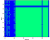 |
Fig. 1. Final accepted data for the GN5 dataset. The data that we used is shown in green, whereas data that do not fulfil the constraints are shown in dark blue and data that fulfill the constraints, but needed to be excluded (as the beam or subband contained too much bad data) are shown in light blue. See Sect. 2.1 for a detailed description. |
2.2. Polarisation analysis
The polarisation analysis was performed using the aperpol4 software (Adebahr et al. 2022a). For a detailed description of aperpol, we refer to Adebahr et al. (2022a). Here, we outline the relevant parts of the aperpol pipeline used in this work.
First, to mitigate the effect of bandwidth depolarisation5, aperpol uses the RM-synthesis on the Stokes Q- and U-cubes that were generated by amosaic. We sampled the Faraday axis in steps of 8 rad/m2 in the range of −1024 rad/m2 ≤Φ≤ 1024 rad/m2. The resolution in Faraday space (δΦ), the maximum observable Faraday scale (Φms), and the maximum observable Faraday depth (Φmax), are provided in Table 2 (per field).
Specifications of RM-synthesis.
The resulting Faraday cubes were then analysed by aperpol to create a polarised intensity (PI) map. To do this, aperpol first locates the maximal value along the Faraday axis. The code then fits a parabola to the peak cell and its two neighbouring cells, such that the defined maxima location in Faraday space is not restricted to the discrete grid of cell values. The PI is then given by the value of the parabolic model maxima, and the RM by the location of the maxima along the Faraday axis.
In the next step, aperpol uses Python Blob Detector and Source Finder (pyBDSF; Mohan & Rafferty 2015), fully automatically, to extract a source catalogue from the PI map. For the source finding, an island threshold of 5.0σ and a pixel threshold of 6.25σ are used, with an adaptive RMS-box to account for the increasing noise at the mosaic’s edges. This creates a polarised source catalogue with one entry for every component, where it is possible for sources with multiple components to be associated, as those components share the same source ID. For each component, an RM value is estimated: as the RM varies strongly towards the borders of a source, the value is taken at the position of the peak flux. Finally, we also ran the pyBDSF software over the TP map that was produced by amosaic, with an island threshold of 4.0σ, a pixel threshold of 5.0σ, and also using the adaptive RMS-box.
The pipeline then cross-matches the PI catalogue with the TP catalogue, using the RA and DEC values from the PI catalogue and a search radius equal to the major axis length of the synthesised beam. Using the matches, we then add total intensity estimates, fractional polarisation estimates, and their uncertainties to each entry in the catalogue of PI sources. Then, using the same cross-matching parameters, aperpol also generated a list of cross-match counterparts in the National Radio Astronomy Observatory (NRAO) Very Large Array (VLA) Sky Survey RM catalogue (NVSS; Taylor et al. 2009). Next, the location of each TP-counterpart was cross-matched with the All-source catalogue from the Wide-field Infrared Survey Explorer satellite (AllWISE; Cutri et al. 2021). The search radius in this match used was the major axis length of the synthesised beam of the TP map. In cases where multiple sources were matched within the search radius, the closest was chosen as the counterpart. Finally, the coordinates of the AllWISE counterparts were cross-matched with the DR16 catalogue of optical sources from the Sloan Digital Sky Survey (SDSS; Ahumada et al. 2020). The SDSS counterpart was identified within the AllWISE resolution of 3.6″. At the end of this process, we have a catalogue of PI sources that are cross-matched to sources in total intensity, AllWISE, and SDSS.
To simplify the visual inspection of each source, aperpol creates a pdf-file for each source, containing various images and overlays. An example of such a file is given in Fig. 2. To enable the construction of these figures, images from WISE, and SDSS g-band, are downloaded.
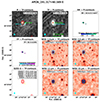 |
Fig. 2. Example pdf-file created by aperpol to inspect each source by eye. The panels show, from left to right, top to bottom: PI map with TP contours, the TP map with PI contours, RM map, FP map, WISE 3.4 μm map with TP contours, WISE 4.6 μm map with TP contours, SDSS g-band map with TP contours, WISE 12 μm map with TP contours, and the WISE 22 μm map with TP contours. Small green x-marks locate the coordinates of the individual components of PI and TP sources in the first two panels, respectively. Large green x-marks locate the position of other PI sources in the first panel and non-cross-matched TP sources in the second panel, whereas large turquoise x-marks locate the coordinate of the PI source in the first or the cross-matched TP source in the second panel. Large red x-marks in the second panel mark the position of NVSS counterparts. Small green and yellow x-marks identify the position of crossmatched WISE and SDSS sources in the corresponding panels. |
During visual inspection of the aperpol images, we modified the catalogue in cases where the automatic cross-matching was not correct. This involved using the interactive functions within aperpol to, for example, remove false detections and false cross-matches, check for new TP or AllWISE cross-matches, or combine PI or TP sources. From this cleaning process, we estimated that the rate of false detections was approximately 3/deg2, with most of these false detections being caused by artefacts around bright sources. Following this procedure, we ended up with one catalogue for each observation, containing a cleaned source list, PI and TP information, and multi-wavelength information for matched counterparts.
2.3. Combined catalogue
To increase the sensitivity of our observations, we can further combine data in the overlapping regions between adjacent pointings, leading to a decrease in the RMS noise in the overlapping areas (see Fig. 3 for the positions of the observations). A full mosaic of the polarised intensity is not possible to construct for several reasons. The first and most critical, problem is the significant computational power required to Fourier-transform all the data for the RM synthesis at once. Secondly, due to the data rejection process described in Sect. 2, a full mosaic would require us to exclude a significant fraction of (otherwise acceptable) data. Additionally, we would also be required to exclude more than half of the subbands of GN5, and about a third of the subbands of GN6, regardless of the data quality, as we cannot combine data observed beyond the original frequency range of the observations (see Sect. 2).
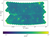 |
Fig. 3. Polarised intensity map of the GOODS-N field. The mosaic was produced following the procedure described in Sect. 2. The numbers highlight the central position of the individual observations used. |
To avoid this unnecessary rejection of data, we instead re-imaged only the overlapping regions between adjacent observations. For the overlaps of GN1 with GN2 (‘GN12’), GN2 with GN3 (‘GN23’), and GN3 with GN4 (‘GN34’), we followed the procedure described in Sects. 2.1 and 2.2. For fields overlapping with GN5 and GN6, we first have to exclude the subbands not covered by either observation (introduced by the change in the frequency window used for observations; see Sect. 2). After the data was adjusted to the same subbands, we followed the same mosaicking and polarisation analysis procedure as for the individual observations.
After this process, six base catalogues (one for each of the observations) were compiled, along with seven additional smaller catalogues for sources in the overlapping regions between observations. To avoid including sources multiple times, we sliced the entire observed area into 13 regions corresponding to the 13 individual mosaics and catalogues. The demarcation of the catalogues and the images was performed using the astropy regions package, which is able to define a polygon-shaped region by defining the polygon’s corners. We defined the slices trying to use the central parts of each individual mosaic. After filtering each individual catalogue by using the slice regions, we can simply stack the filtered catalogues to one final catalogue that we call the slice catalogue. Using the same region-objects, we also cut the polarised intensity map and its noise map. The leakage of Apertif data are currently not known in detail and no correction is available. However, as Adebahr et al. (2022a) found the instrumental polarisation of Apertif to be on the order of less than 1%, we excluded sources with FP ≤ 1% from our analysis to avoid including sources that show purely instrumental polarisation. A correction of the polarisation bias on our data is not yet available. Both effects, instrumental polarisation leakage as well as polarisation bias, are stronger towards the edges of each individual mosaic. To mitigate those effects, we also applied a mask that excludes all regions where the primary beam response is below 20%. This procedure shrinks the mosaic to an area of 47.4 deg2 containing 1468 components in 1185 sources, as shown in Fig. 3.
2.4. Completeness
Due to the complex pipeline used to generate our final sample, we expect that the sample has a number of similarly complex selection functions imprinted upon it. Such selections can introduce biases to analyses of population properties. We investigate the selection functions imprinted on our sample using synthetic source injection, a methodology common in the optical astronomical literature since the mid-1980s (see, e.g., McClure et al. 1985). Our implementation of this process was designed to model the probability of detecting sources after the image reduction and extraction process. As such, we started by injecting point sources into the Q- and U-frequency cubes of all datasets, prior to running aperpol. The polarisation angle was chosen to be constant at 45° over all wavelengths, corresponding to RM = 0, so the flux is uniformly distributed between the Stokes parameters Q and U, following the standard equation  . The mock sources themselves were generated by using the astropy.modeling.models package.
To estimate the flux-dependence of completeness in our dataset, we injected sources with a range of different polarised intensities. For each simulated flux, multiple sets of 200 sources were added into the observed Stokes Q- and U-image cubes, at random locations. We then ran our aperpol pipeline on each injection set, using the same input parameters as used in the creation of the actual data catalogue. While for the analysis the PI_cat_final.txt aperpol output file was used, here we use the more preliminary catalogues PI_cat_clean.txt, which was generated before any of the cross-matches performed by aperpol. As part of the cross-match with total intensity, multiple polarised sources that are cross-matched with the same total intensity source are combined to one source (this is for instance important for resolved FR II type sources). By using the PI_cat_clean.txt catalogue, we avoided mismatches between the input and the recovered catalogue that might occur due to such source combinations. Since the sources were injected at random locations over the full image, all catalogues used were sliced by the same region slices as those used for the combination of the individual catalogues.
To compute the completeness of the dataset as a function of input flux, we must estimate the fraction of injected sources that were subsequently extracted from our imaging. We do this by starting with the set of all injected sources, ℐin. As the sources are randomly distributed over the image, we first exclude all injections that land on-top of already existing sources present in the original (the non-injected) extraction catalogue  (where the hat denotes a sample that has undergone an extraction selection function). This gives us the set of all injected sources that could have been detected ℐpos:
 (1)
(1)
where the superscript c denotes the complement of that set (in this case, all sources that are not in the originally extracted catalogue  ). This rejection was performed using a simple sky-match, with a matching radius equal to the synthesised beam major-axis length. We also performed a cleaning of the ℐpos catalogue, removing an injection from pairs that were randomly placed within one beam of each other (and would therefore be blended). In practice, two sources being injected so closely is exceedingly rare. This cleaned catalogue therefore contains only injections that are alone and separated from pre-existing data sources: we call this set ℐclean.
For each injection realisation, the list of all extracted sources ( ) contains three components: sources from the original data extraction (
 ), injected sources that we are able to extract (
 , our true positives) and false detections (
 , our false positives):
 (2)
(2)
 (3)
(3)
This also provides us with a false-negative rate, which is simply the set of all injections that are not extracted:
 (4)
(4)
Table 3 gives an exemplary overview of the sizes of these various sets as a function of flux, along with the number of realisations of each set that was made, for the case of GN5. Additionally, Fig. 4 shows graphically the fraction of true positives as a function of flux. This therefore provides a demonstration of the empirically estimated completeness that we are measuring as a function of true flux for a single GN observation.
Completeness of the mock data of GN5.
 |
Fig. 4. Completeness (true positive rate) given as a function of inserted PI flux. For all individual fields. |
To make the completeness function useful in our later application to source count measurements (see Sects. 4 and 5.2), we fit the completeness with a function of the form:
 (5)
(5)
where compfit is the completeness, f is the inserted polarised intensity flux, and a1, a2, a3, and a4 are the fitting parameters that we are aiming to optimise. The best-fit values, calculated for each individual dataset, are given in Table 4. While the fit provides a good estimate of the completeness at low fluxes, it can exceed 100%, which is not physical. We therefore defined a flux limit f_lim for each individual dataset, above which no completeness correction is needed. Therefore, the completeness comp over all flux ranges can be written as
 (6)
(6)
and is determined for each individual field.
An added complication in the estimation of completeness using an injection simulation is the systematic variation of sensitivity over the mosaic. We can calculate the relative effective area by computing the fraction of pixels in which a source of flux f would be detectable, given the RMS noise of the image and the used extraction threshold of 6.25σ. Since all individual fields are of different size, these values are normalised by the fields’ total area. Comparing the completeness of the different fields to their relative effective area as a function of flux (see Fig. 5), both trends appear similar, indicating that the major effect on the completeness is indeed the noise distribution of the image. We aim to apply this correction to the source counts, which also include an area normalisation. It is therefore convenient to avoid distinguishing between area and completeness correction but to use one correction that includes both. However, to account for the different RMS noise distributions when applying the completeness correction to the source counts, we added a secondary correction to re-weight the completeness function by the relative area.
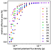 |
Fig. 5. Effective area in which a source with a given flux would be detectable due to the noise. |
The final completeness correction applied to the source counts corrects for the field’s (in which the source was observed) completeness, weighted by the ratio between the respective field’s effective area and the combined effective area from all fields for a given flux. In this way, we account for the probability of each source to be detected and for the inherent differences between the individual fields’ sensitivity profiles.
2.5. Flux accuracy
The mock data, discussed in Sect. 2.4, not only allows us to investigate the completeness of our source finding, but also provide a tool to measure the accuracy of our fluxes. Adebahr et al. (2022a) investigated the flux measurement accuracy of Apertif data by comparing flux and RM values of Apertif and NVSS sources that were detected in both, NVSS and the SVC sample. However, due to the NVSS being less sensitive than current surveys like AWES, only sources with polarised fluxes brighter than ∼4 mJy were used in this comparison, limiting the flux validation to high-flux sources. By using our simulations of faint sources, we extended this flux validation into the sub-mJy-regime.
As a measurement of the flux measurement accuracy, we calculated the relative deviation between injected and detected flux Δf = (PIinserted − PImeasured)/PIinserted as a function of injected flux. pyBDSF provides multiple methods of calculating the flux of a source from the input image. The one that is used throughout aperpol and, therefore, the one used for the flux validation done by Adebahr et al. (2022a), is the ‘Total_flux’, which is the integrated flux of the source, calculated by pyBDSF fitting Gaussians to each component. The ‘Peak_flux’, which gives the peak flux for each component, is also kept in the final output of aperpol. While this flux is not a good measure for extended sources, it should be in good agreement with the ‘Total_flux’ and the injected flux for our simulated sources, as all of those are point sources. Both of the aforementioned flux measurements are based on the source being fitted by one or multiple Gaussians. While this is a suitable approach for Stokes I, Q and U, the statistics in PI are not Gaussian, so this might lead to biases. For this reason, we also compare the inserted flux to the ‘Isl_Total_flux’, which is the summation of all pixel values within the island, as defined by pyBDSF, while no Gaussian fit is used. The median Δf as a function of injected flux is shown in Fig. 6 for all three different fluxes. While we can confirm the flux validity shown by Adebahr et al. (2022a) for fluxes higher than ∼4 mJy, we find significant offsets between injected and measured fluxes for sub-mJy fluxes; in particular, the ‘Total_flux’ diverges strongly from the actual source flux, by underestimating the flux by up to 50% at around 125 μJy. We attribute the large offset between injected and measured flux for the ‘Total_flux’ and the ‘Peak_flux’ to the assumption of the sources being of Gaussian shape. While both aforementioned flux measures do not provide a valid measure for the actual sources flux at the sub-mJy-level, the Δf value based on the ‘Isl_Total_flux’ is rather close to zero for fluxes above ∼90 μJy. For this reason, we decided to use the ‘Isl_Total_flux’ throughout this paper as a measure of the polarised flux, while excluding sources below 90 μJy from our analysis.
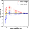 |
Fig. 6. Median difference of measured flux compared to injected flux (Δf) as a function of the injected flux. The black line gives Δf = 0, where both fluxes are the same. |
We note that the large error bars of all fluxes can be attributed to the fact that our source injection is done in the image plane, rather than in the uv-plane, and the sources are injected on top of the background noise. Thus, their flux is scattered by the positive or negative noise flux in the individual Q- and U-cubes.
Here, the observed discrepancy between fitted flux and actual flux, even for point sources, highlights the need to improve source finding and measurement for polarised intensity data. While our solution, as well as other approaches to source finding, such as the study from O’Sullivan et al. (2023), are suitable for current polarisation surveys, upcoming SKA surveys will bring new challenges for source finding and flux measurement in polarisation. Currently, methods of source finding in Faraday depth only provide peak flux information. While this is a good indicator for point sources, it is of limited use for extended structure that will be more common in future polarisation surveys due to their increasing sensitivity (see eg. Adebahr et al. 2022a). This also limits the use of our approach, since when using the pyBDSF ‘Isl_Total_flux’ (in contrast to using the ‘Total_flux’), we cannot handle different sources in overlapping islands. This upcoming challenges highlight the need for a source finder and measurement software, tailored for polarised intensity data.
2.6. Adjustments to aperpol
As mentioned earlier in this paper, it is only the ‘Total_flux’ and the ‘Peak_flux’ that were propagated though aperpol. For this reason, we adjusted aperpol to make the ‘Isl_Total_flux’ usable. To allow for backwards compatibility, we did not simply replace the ‘Total_flux’ by the ‘Isl_Total_flux’, but kept both by inserting additional columns. All columns that were based on the pyBDSF ‘Total_flux’ were renamed, for clarification. A list of the columns that changed or were added in comparison to Adebahr et al. (2022b) as well as a detailed description of all changes are given in Appendix A and B. We ran all our data using this most up-to-date version of aperpol6 and take the ‘Isl_Total_flux’ based PI_Isl column for the flux of our sources.
3. Results
We detected 1182 polarised sources brighter than 90 μJy in 1465 components, in an area of 47.4 deg2. This makes up 8.1% of all TP sources being polarised, with a median fractional polarisation of 5.68 ± 2.74%. Compared to previous surveys, we covered a much larger area with a sensitivity comparable to the most sensitive deep fields. This allows a significantly improved statistical analysis. Our values are in good agreement with those previous works, where median fractional polarisations of 4.8 ± 0.7% (Taylor et al. 2007), 6.8 ± 0.7% for resolved, and 4.4 ± 1.1% for compact sources (Grant et al. 2010), 6.2% (Hales et al. 2014a), 6.2% (O’Sullivan et al. 2015), and 5.4% (Berger et al. 2021) were found in deep field investigations. We note that the median fractional polarisation of 4.70 ± 0.14% reported by Adebahr et al. (2022a) in their work on the Apertif SVC fields was calculated using the old version of aperpol, so the polarised flux was likely underestimated. Also, our percentage of sources being polarised is in good agreement with previous works with values of 10.5% (Taylor et al. 2007), 14.2% (Grant et al. 2010), 5.8% (Hales et al. 2014a), 8.8% (Berger et al. 2021), and 10.57% (Adebahr et al. 2022a). The small differences will be discussed in detail in Sect. 3.2.
3.1. Source classification
First, we want to investigate the nature of our sources. In particular, we want to check for the detection of polarised emission from star formation dominated galaxies, as this is currently unobserved in untargeted surveys. To this end we use the mid-infrared-radio-correlation (MRC, e.g. Cohen et al. 2000; Elbaz et al. 2002): Vaddi et al. (2016) found a correlation between the mid-infrared-flux and the total radio emission at 1.4 GHz where the total radio flux can be explained by star formation only. This correlation is not as strong as the far-infrared-radio-correlation (FRC; e.g. Condon et al. 1982; Appleton et al. 2004), but it gives a good estimate of the origin of the radio emission being either star formation or AGN activity. Figures 7 and 8 give the total radio flux density over the flux density in the two MIR bands from WISE. The respective MRC is shown in each figure as the blue dashed line, while the dotted lines gives the MRCs uncertainty. We would assume a source, where the radio flux is dominated by star formation, to be located within the MRCs uncertainty range. For both, the 12 μm and the 22 μm plots, all sources have a radio flux much higher than explainable by the MRC. So, as expected, there is currently no evidence that any of our polarised sources are dominated by star formation.
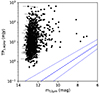 |
Fig. 7. Radio flux compared to MIR flux for our sources with a 12 μm counterpart from allWISE. The dashed line gives the MRC from Vaddi et al. (2016) and the dotted lines gives its uncertainty range. |
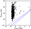 |
Fig. 8. Radio flux compared to MIR flux for our sources with a 22 μm counterpart from allWISE. The dashed line gives the MRC from Vaddi et al. (2016) and the dotted lines gives its uncertainty range. |
We note that Vaddi et al. (2016) remeasured the WISE fluxes for their analysis, while we use allWISE data. WISE data was found to underestimate the fluxes slightly. Even with a slight underestimation of the IR flux, our sources would still remain above the MRC.
The radio fluxes stronger than the MRC can be explained by the AGN activity. As we did not find any hint for our polarised sources being dominated by star formation, we assume all our sources to be AGN. However, we note that this analysis is only statistical and that not all our sources have IR counterparts. We have IR counterparts for 1023 of our polarised sources.
3.2. Fractional polarisation behaviour
The behaviour of fractional polarisation over the total flux density is an important property for analysing the characteristics of polarised sources, as well as for the interpretation of source counts (see Sect. 4). In previous works, the behaviour of fractional polarisation with total intensity was discussed (see e.g. Tucci et al. 2004; Mesa et al. 2002; Taylor et al. 2007; Grant et al. 2010; Hales et al. 2014a; Berger et al. 2021) and it was ultimately determined that the median fractional polarisation of sources is higher towards lower total intensity flux densities. Rudnick & Owen (2014) found this trend to end for TP < 5 mJy. Hales et al. (2014a) explained this trend to be an effect of the sensitivity limitation in PI, as to this limit, only sources with a high fractional polarisation exceed the necessary threshold to be detectable. However, Rudnick & Owen (2014) offered a detailed discussion on how this bias affected the conclusions of an anti-correlation between the fractional polarisation and total flux density in previous works, noting that even at high total intensity fluxes, the bias can still affect the data.
The selection bias was confirmed by the analysis of Berger et al. (2021), even though they found significantly varying trends between different deep field observations. In that paper, the authors argued that sample variance is the primary driver of these differences, due to the small fields as well as the special characteristics of the deep field regions. With our data we have been able to reach equivalent (or higher) sensitivities compared to the aforementioned works mentioned in Berger et al. (2021), but more than eight times their survey area, enabling us to investigate this effect in more detail.
Using the additional SVC data from Adebahr et al. (2022a), which cover five non-adjacent fields, we can also include a comparison of six different regions on the sky. However, as mentioned before, this data was analysed using the first version of aperpol; thus, it suffers from the underestimation of the polarised flux at sub-mJy-levels. To be consistent, we also reran the necessary aperpol steps on the SVC data.
As the fractional polarisation is the ratio of the polarised flux density and the total flux density (FP = PI/TP), it is given by the slope of PI over TP. In Fig. 9, we show the median polarised intensity over the geometric mean of the total intensity bin for the GOODS-N and the SVC data, as well as for a combination of both to achieve better statistics. The red line represents a constant FP of 4.48% (the median FP of the GOODS-N data, when excluding all sources with TP ≤ 10 mJy, to account for the selection bias). For the lowest flux bins (below ∼5 mJy), the data are dominated by the selection effect, preventing the detection of sources that would lie below the black-dashed line (90 μJy). For higher total intensities those sources become less significant and, thus, the data converge to the red line. We have thus determined a linear correlation between PI and TP. The Pearson correlation coefficient for this resulted 0.90 with a p-value of 2.45 ⋅ 10−5.
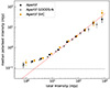 |
Fig. 9. Polarised intensity binned over the sources’ total intensity. The red line gives the polarised intensity for a given total intensity assuming FP = 4.48%, the black line represents the sensitivity limit. |
The next subsections will give an overview on how the median fractional polarisation was previously found to behave with the total power flux for different deep fields and how this can be compared with our findings. The effect of sample variance is discussed below.
3.2.1. Comparison to literature data
In Fig. 10, we compare our data (grey), the SVC data (orange) and the combination of both (black) with data of Mesa et al. (2002), Tucci et al. (2004), Taylor et al. (2009), Grant et al. (2010), Subrahmanyan et al. (2010), Stil et al. (2014), Rudnick & Owen (2014), Hales et al. (2014a), and Berger et al. (2021). The various aspects of this plot will be discussed in the following (sub)sections.
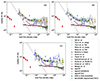 |
Fig. 10. Median fractional polarisation over total intensity. Data from the literature compared to our Apertif GN, SVC data and the combination of both in plot (a), the grey error bars to the full Apertif sample represent the sample variance, the area in which the individual bootstrap samples are located is visualised in grey. Plot (b) presents the individual GN and SVC fields as lines. Plot (c) shows the effect of bandwidth and beam depolarisation on selected data sets from the GN and SVC data. The dotted line in each plot gives our detection limit of PI ≥ 90 μJy. |
The three lowest TP flux density bins show the selection effect that was already discussed by Hales et al. (2014a) and Berger et al. (2021) (see Sect. 3.2). This sensitivity limit is shown by the black dashed line, using our 90 μJy limit. Due to the limited sensitivity in PI, we are not able to detect or measure any sources below that line, as they would fall below our detection threshold.
For the highest total intensity flux densities, the GOODS-N and SVC data scatter around the combination of the data randomly but within their respective errors. We attribute this to the quite small number of high flux sources above ∼200 mJy. For flux densities below this value, the trend seen in the SVC and the GOODS-N data is in good agreement. For the flux range above ∼10 mJy, the fractional polarisation is for all Apertif data relatively constant over total intensity flux density. To account for the sources without detected polarised emission, we employed the Kendall’s tau test for censored data from Flury et al. (2022)7. We include upper limits for all sources that were not detected, including those sources with FP < 1%, that were excluded from our catalogue (see Sect. 2.3. We find τ = 0.026 and a p-value of 4.57 ⋅ 10−7. While this p-value implies a statistically significant correlation between FP and TP, the correlation has an extremely low amplitude, so FP does increase slightly with increasing TP, but the correlation has a very flat slope. We can therefore approximate our median FP by a constant value over our observed total intensity range.
3.2.2. Sample variance
Sample variance, so the intrinsic differences of an observed sample, for instance the difference between observing a cluster to a void, might also affect the fractional polarisation. Berger et al. (2021) claimed this to cause the observed different trends.
In Fig. 10b, we compare the median fractional polarisation behaviour of the individual GOODS-N and SVC fields to other deep field observations, as Berger et al. (2021) highlighted differences between different deep fields.
To investigate the effect sample variance has on our data, we use the bootstrap method (Tibshirani & Efron 1993) on the combination of our GOODS-N and the SVC data. To this end, we cut our complete sample (GOODS-N and SVC catalogues) into 19 subsamples, each covering an area of about 4.6 deg2. This value was selected to enable a minimal loss of area. We then resampled 1000 complete bootstrap-samples by randomly drawing 19 subsamples with replacement, for each of the bootstrap-samples. For each of the 1000 bootstrap-samples, we then calculated the median fractional polarisation in the same ten total flux density bins, as we did for the complete Apertif-sample. The sample variance is calculated for each of the bins and corrected for the Poisson error resulting from the number of bootstrap samples used. Figure 10 shows the sample variance as light grey error bars of our black Apertif data points. We only plot those error bars for our complete Apertif sample data. The distribution of the bootstrap samples median fractional polarisation is also shown in Fig. 10a.
It is visible, that most data points, from the different deep fields are in the greyish area, which represents the bootstrap samples. Sample variance for smaller fields is even stronger. Thus, we concluded that the different trends observed in different deep fields can be explained by the effects of sample variance.
Apart from the effects of small number statistics and sample variance, we observe an approximately constant fractional polarisation over the observed total intensity range, which does not suffer from the sensitivity bias. This is in agreement with the findings of Hales et al. (2014b). We thus assume this to be valid down to ∼1 mJy (the limit given by Hales et al. 2014b).
3.3. Fractional polarisation distribution
We present a model to describe the distribution of fractional polarisation for our GOODS-N sample. As discussed in Sect. 3.1, we do not find any indication for our sample to contain sources whose polarised emission is dominated by star formation, leading to the restriction of this model to be only valid for AGN sources. In Sect. 3.2, we discuss the fractional polarisation to only be weakly dependent on the sources’ total intensity, so we can assume FP to be constant over TP down to TP ∼ 1 mJy.
We assume that the data follow a log-normal distribution with the probability density function (PDF) of the form
 (7)
(7)
where e is Euler’s number, while μ and σ refer to the mean and standard deviation of the corresponding normal distribution.
Since the discussed selection bias causes a large number of high FP sources without their low FP counterparts to be present in our sample at fluxes TP ≤ 10 mJy, resulting in an artificial increase in the overall median FP, we only account for sources above this threshold when fitting the PDF.
Figure 11 shows the distribution of the fractional polarisation found in our sample. To find the best-fit values, we performed two fits to the data: The first uses the relationship between log-normal and normal distribution; if our sample X is log-normally distributed to the basis 10, then the sample Y = log10(X) is normally distributed. Using this relationship, we can obtain the parameters μ and σ by fitting a normal distribution to our Y sample (shown in green). Our second method is a direct fit of Eq. (7) to our sample, presented as the red line in Fig. 11. The values and the corresponding R2 parameters of the fit are given in Table 5.
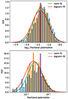 |
Fig. 11. PDF of the fractional polarisation of the GN sources. The distribution of all detected sources in our sample are shown in blue (we note that the sources with FP ≤ 1% are excluded from all analysis since those values are very uncertain and probably heavily influenced by polarisation bias and leakage), while the orange sample (FP ≥ 1% and TP ≥ 10 mJy) is the sample used for fitting. |
4. Source counts
In this work, we present the Euclidean-normalised differential polarised source counts as well as the cumulatively polarised source counts. We account for the completeness of our data (see Sect. 2.4) by weighting every source with the completeness of its flux. As discussed in Sect. 2.4, this correction does include the area correction, as we injected sources over the entire field and applied no correction for sources that were injected in regions where they are not detectable due to the local noise. Thus, we only have to normalise the counts for the entire area covered.
To account for the slight variations in completeness between the individual fields, which we attribute to the different effective area distribution, we weigh the entire area by the ratio between relative effective area of the field to the full relative effective area:
 (8)
(8)
where Anorm is the area normalisation factor applied to the source counts, A is the area, the superscript eff denotes the effective area, the subscript i denotes the area of the source’s field, and all refers to the full field. For reasons related to the computing time, the area is not calculated for each individual flux, but on a bin-mean basis, this approximation only breaks for the lowest fluxes, where the effective area differs strongly within one bin.
Since the completeness becomes statistically more uncertain towards lower completeness levels as well as our area correction becoming more error-prone, we decided to exclude all sources with a completeness of less than 20% from our source counts. To propagate this through the area normalisation, we first calculate the completeness of the source in its field via Eq. (6). If this was higher than 20%, we calculated the full (and effective) area ( ) as the sum of all fields’ (effective) areas with completeness higher than 20%. This correction is applied to both cumulative and Euclidean-normalised differential polarised source counts.
4.1. Cumulative polarised source counts
In Fig. 12, we present the cumulative polarised source counts for our GOODS-N data. The grey circles give the source counts for our GOODS-N data. We also present the cumulative counts of the combined data of the five Apertif SVC fields as the orange data points, since we do not have a completeness correction for these fields, we apply the completeness from GN4, as this field’s area distribution fits those of the SVC fields best. We present the combination of our combined GOODS-N catalogue with the SVC catalogue as the black data points.
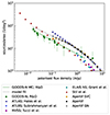 |
Fig. 12. Cumulative polarised source counts of the GN-field (grey), the SVC-fields (orange), and the combination of both (black), compared to data from the literature. |
For high flux densities, our findings are in good agreement with the data of Hales et al. (2014a). Due to our high sensitivity threshold, we are able to just overlap with the flux regime where Rudnick & Owen (2014) published counts from their deep investigation in the GN field. Slight differences can be explained by the effect of sample variance, which we discussed in the context of fractional polarisation behaviour. Even though we are not able to present source counts for the lowest fluxes, we observe a flattening trend of the source counts below ∼1 mJy. This is in agreement with the flattening observed for lower fluxes by Rudnick & Owen (2014), starting at the same flux density. However, this is in contrast to the counts of Hales et al. (2014a) and Stil et al. (2014), which show no such trend, but do show the same steep slope for flux densities below ∼1 mJy than for higher fluxes. It is worth noting that different works have applied different corrections to their source counts. In agreement with Rudnick & Owen (2014), we applied an experimental completeness correction (see Sect. 2.4 for details), by weighting every source with the completeness of its respective flux. Hales et al. (2014a) applied a correction for the resolution and Eddington bias, where the latter is based on the total intensity source counts and might therefore bias the counts to the shape of the total intensity counts.
4.2. Euclidean normalised polarised differential source counts
For the calculation of the Euclidean-normalised polarised differential source counts, we also include the resolution bias following Prandoni et al. (2018), as well as our own completeness correction. In Fig. 13, we present the source counts for our combined final catalogue of the GOODS-N field as well as for the combination of all Apertif SVC fields. We also model the source counts, by convolving the source count model from Hopkins et al. (2003) with our fractional polarisation PDF (see Sect. 3.3), shown as the red line. The blue and turquoise data points are component counts taken from Hales et al. (2014a) for ELAIS-S1 and the CDF-S. The cited authors also predicted the solid black line for component counts based on the model of Hopkins et al. (2003). Even though Hales et al. (2014a) present component and not source counts, both should be comparable at the considered resolution (Hales et al. 2014a). We note that in contrast to Hales et al. (2014a), who fit their PDF model to both, the direct source distribution and the source counts, our model is only directly fitted to the distribution of fractional polarisation. However, both models are in good agreement (excluding the highest fluxes where the sampling is sparse), proving our calculated PDF to be suitable. For the highest fluxes, our source counts agree with the findings of Hales et al. (2014a), while they follow a steep slope towards lower fluxes. At low fluxes, our source counts drop to the much lower source counts of Stil et al. (2014). Such a steep slope was only found by Berger et al. (2021).
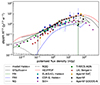 |
Fig. 13. Euclidean normalised polarised differential source counts for the GN field (grey), the Apertif SVC (orange) fields and both combined (black), compared with data from the literature. |
5. Discussion
In Sect. 3.2 we present the behaviour of median fractional polarisation over total flux density of our sources and the SVC data from Adebahr et al. (2022a), compared to other deep field observations from the literature. In agreement with Berger et al. (2021), we have found different trends for the different individual fields. We can explain these differences by the effects of sample variance and small number statistics in the individual fields. After accounting for these discrepancies, our observed trend for the combination of the Apertif SVC and GOODS-N data is in quite good agreement with all previous small deep field observations. In this section, we also discuss the effect of these findings on the interpretation of our source counts, we presented in Sect. 4.
5.1. Technical effects on fractional polarisation
The increase in the fractional polarisation towards low total intensity flux densities due to the sensitivity limitation can also be seen in the decrease in the fraction of TP sources that are detected in polarised intensity (Adebahr et al. 2022a). For TP ≥ 10 mJy the effect of the sensitivity limitation in Fig. 10a is not visible any more and more than 50% of the TP sources have polarised counterparts. When excluding the flux density ranges below this cut-off, we find a constant median fractional polarisation of 4.48 ± 2.21%. When we are not excluding the lowest flux density ranges, we find a median fractional polarisation of 5.68 ± 2.74%. As expected the median FP is a bit lower when excluding the sensitivity affected flux regions, however (thanks to the median being relatively stable against outliers), the difference is not significant compared to the overall uncertainty. A constant trend of FP is also confirmed by the linear correlation between polarised and total intensity flux densities, while Kendall’s tau implies FP to be weakly correlated with TP.
Stil et al. (2014) also found a weak dependence of fractional polarisation on the total flux density by using the NVSS and a stacking technique to increase the sensitivity and avoid completeness effects. We note that the slope found by those authors (log10(FP)∝ − (0.051 ± 0.004) log10(TP) is very small, and thus within our uncertainties.
Comparing our data to the data of Stil et al. (2014), Tucci et al. (2004) and Mesa et al. (2002), we find a large offset in fractional polarisation by a factor of about 2, which is in agreement with other deep field studies. A major difference between our investigation and the studies mentioned above, is the way the median is calculated. While we only account for sources that have detected polarisation, the other studies include all sources above a given total intensity limit, thereby also including sources without significant polarisation and pushing the median fractional polarisation to lower values. A comparison of those values is thus not straight forward and beyond the scope of this work.
It is worth to note, that all three works use the NVSS and the later two its direct measurements, so they only include the brightest sources down to ∼100 mJy. The usage of the NVSS could introduce biases relative to our work with Apertif, such as beam- and bandwidth depolarisation, which will be discussed in the following.
The effect of bandwidth depolarisation was already discussed by Condon et al. (1998) to be very low due to the low RM values of the sources. However, assuming our data to be free from bandwidth depolarisation due to the usage of the RM-Synthesis, we calculate the effect of bandwidth depolarisation on one of our fields (SVC4, as this is the closest to the galactic plane, showing the strongest impact of Faraday rotation). We do so using
 (9)
(9)
where RM is the rotation measure, λ0 is the observed wavelength, ν is the central frequency, and Δν is the bandwidth.
As the synthesised beam of the NVSS of 45″, used by Tucci et al. (2004) and Mesa et al. (2002), is much larger than the beam of our Apertif data with about 15″ × 18″, another possible explanation for this offset could be beam depolarisation. Stil et al. (2014) used images with an even lower resolution of 60″. To investigate the influence of beam depolarisation, we reimaged the data of two GOODS-N observations to a synthesised beam of 45″ × 45″, prior to running the polarisation analysis on the data. We decided to apply this smoothing to the most sensitive fields, GN5 and GN6.
The results of this are shown in Fig. 10c. No significant difference between smoothed and original data is visible in Fig. 10a. Thus we conclude that beam depolarisation cannot be the reason for the lower observed fractional polarisation. The green squares with applied bandwidth depolarisation approximation show a bit lower fractional polarisation on average. However, in agreement with Condon et al. (1998) this effect is not very strong and is even within the natural variation of small sample statistics. Neither the bandwidth nor beam depolarisation can explain the offset of about 2–3% between the observed fractional polarisation of the data from Stil et al. (2014) and our Apertif data.
This offset might partially originate from not correcting for instrumental polarisation in the Apertif data. Adebahr et al. (2022a) showed that the instrumental polarisation of Apertif is on the order of up to 1%. Even though we excluded all sources that show a fractional polarisation of less than 1%, we did not apply any correction on the remaining sources. Thus, an overestimation of the fractional polarisation of the Apertif sources cannot be excluded. However, a 1% overestimation would not explain the entire offset between our data and the Stil et al. (2014) data. It is likely for this offset to result from the differences in treating non-detections in polarised intensity. We note our observed median fractional polarisation is, however, in good agreement with the findings of Hales et al. (2014a) and Grant et al. (2010), but higher than found by Berger et al. (2021) and Subrahmanyan et al. (2010). As explained in Sect. 3.2, this may be an effect of sample variance.
5.2. Source counts
In Sects. 4.1 and 4.2, we presented cumulative source counts as well as Euclidean-normalised differential source counts in polarised intensity. As shown in Sect. 4.1, our findings are also in good agreement with other data. While for high flux densities, we find our Euclidean normalised source counts to agree with the findings of Hales et al. (2014a), we find a steeper slope towards lower flux densities, which is in agreement with the work of Rudnick & Owen (2014).
To compare the observed flattening in our cumulative source counts to that observed by Rudnick & Owen (2014) we fit the power-law distribution, assumed by that work as
 (10)
(10)
where P0 = 0.03 mJy, to our data. For fluxes below 1mJy, we get best fit values of N0 = 66.5 ± 1.7, while this is higher than the value of N0 = 45.4 found by Rudnick & Owen (2014) for their sample of sources at 1.6″, it is in good agreement with the estimate of N0 = 68 the authors extrapolated for a resolution of integrating over the entire source at 10″. By finding α = −0.54 + / − 0.013 for PI ≤ 1 mJy and α = −1.01 ± 0.04 for PI > 1 mJy, we confirm the shift in cumulative count slope, found by the aforementioned work, who found α ∼ −0.6 PI ≤ 1 mJy and α = −1.4 for PI > 1 mJy. Our fit is shown as the gray line in Fig. 12.
In contrast to the study of Hales et al. (2014a), we did not rely on a correction based on total intensity counts but on an empirical correction for the completeness. This is similar to the approach presented by Rudnick & Owen (2014). These different corrections might cause an offset, as discussed below.
The offset between the Hales et al. (2014a) source counts and those from Stil et al. (2014) can be explained by the low fractional polarisation observed by Stil et al. (2014). Those authors extrapolated the Wilman et al. (2008) total intensity model by convolving it with their fractional polarisation distribution, as the stacking approach did not allow for directly obtaining polarised source counts.
The extrapolation of total intensity source counts to polarised source counts is shown by the red line, where we convolved the model of Hopkins et al. (2003) with our polarisation distribution function (Eq. (7)).
In Fig. 14 we also show counts assuming other constant median fractional polarisation in magenta, where FPmed = 2.2% the median from Stil et al. (2014) is used, in yellow, where we use FPmed = 10% to show the effect of different fractional polarisation. From the three different FP values used, we can see that for a flux-independent FP, the slope will not depend on the actual FP assumed. Different FP only result in an offset of the source counts. It is clear that our red line is in good agreement with the black line representing the model from Hales et al. (2014a), while the magenta line is in good agreement with the findings of Stil et al. (2014).
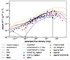 |
Fig. 14. Euclidean normalised polarised differential source counts from Apertif data and the literature, compared to estimates of source counts based on the total intensity catalogue of one GN-field, convolved with our fractional polarisation PDF, assuming different median FP values. |
Nevertheless, none of those counts show the steeper slope we observe with our measured Euclidean normalised polarised source counts, which fit the counts from Hales et al. (2014a) well only for high fluxes; at around 1 mJy they fall down below the counts of Stil et al. (2014). A comparable behaviour was only observed by Berger et al. (2021) who found even lower counts. This difference between our findings and those of Berger et al. (2021) can be explained by the effect of completeness that was not (in contrast to this work) corrected for. By calculating the source counts without completeness correction, we confirmed the offset between Berger et al. (2021) source counts and ours, to be fully explained by the missing completeness correction.
An offset between directly measured PI source counts and those derived from TP counts might thus be explained by two effects. One is a different observed fractional polarisation, while the other originates in a different fraction of total intensity sources being observed in polarisation. With our extrapolation of PI counts from TP counts, we assumed all sources detected in total intensity to be polarised by the same fractional polarisation PDF. This is in good agreement with previous works, which did not differentiate between those two effects, but only accounted for a flux dependency of the fractional polarisation. In our work, the work of Hales et al. (2014a), and of Berger et al. (2021)FPmed is calculated only for the sources with measured polarised intensity and does not account for the sources without measured polarised emission at all. Our finding that FP does at most change slightly with TP does not therefore entail any information on the fraction of sources being polarised. As mentioned before, Hales et al. (2012) applied corrections based on the total intensity source count model from Hopkins et al. (2003). This also includes the assumption that the fraction of sources being polarised is not dependent on flux. This effect might be the source of the offset between their measured polarised source counts and those presented in this work.
The observed decrease might thus result from a probability distribution for a source to be polarised, which is dependent on the total intensity flux density of the sources. We have observed fewer sources being polarised to lower fluxes. In agreement with Rudnick & Owen (2014), this can be explained by the predicted shift in source composition from bright FR II sources at the brightest fluxes to FR I sources dominating at about 30 mJy and, finally, to star-forming galaxies becoming more significant at about 1 mJy in total intensity source counts (Taylor et al. 2015).
Assuming the above-mentioned change in the AGN population from highly polarised AGN to low polarised AGN would thus result in a lack of polarised sources in the source counts for the flux regions of transition between those populations. The low-polarised sources will appear in the source counts only at lower polarised fluxes, while the high polarised sources remain in the predicted flux regime. This is in agreement with our observed source counts and the interpretation of Rudnick & Owen (2014).
6. Summary and outlook
Using six Apertif observations, we were able to generate polarised intensity maps covering an area of 47.5 deg2, while reaching central RMS noise values between 8 and 12 μJy. In this area, we find 1185 polarised sources. All sources were cross-matched with total intensity, allWISE, SDSS, and NVSS data. Using the MRC, we demonstrate that we did not find any hint for our polarised sources to be dominated by star formation. Thus, we claim all these sources as AGNs.
To investigate the source counts, we first analysed the behaviour of fractional polarisation over total intensity. We find the fractional polarisation to change only slightly with total intensity, making an approximation by a constant suitable. We also find an offset comparing our data and previous deep field investigations to the stacking analysis of Stil et al. (2014). As in previous deep field investigations (see Taylor et al. 2007; Grant et al. 2010; Hales et al. 2014a; Berger et al. 2021), different trends were observed; thus, we included the data of Adebahr et al. (2022a) and used the bootstrap method to investigate the effect of sample variance on our data. We found this effect, in combination with poor small sample statistics of previous deep fields, to explain the observed differences. However, this effect is not large enough to explain the observed offset to Stil et al. (2014).
We present Euclidean-normalised differential as well as cumulative polarised source counts. We observe a steeper slope than expected by previous works, where the polarised source counts were calculated based on the total intensity counts (Stil et al. 2014; O’Sullivan et al. 2008) or corrections based on the total intensity counts were applied (Hales et al. 2014a). This steep slope fits to the flattening that Rudnick & Owen (2014) observed in cumulative counts. We attribute this to a change in the AGN population, from highly polarised AGN in the bright regime to low polarised AGN at low total fluxes.
Our data cover the LOFAR GOODS-N deep field and in a future work, these data will be used to analyse the depolarisation properties of the polarised sources in this field by combining L-Band and 150 MHz LOFAR data. With our work, we demonstrate that Apertif can serve as a powerful tool in investigating the faint polarised radio sky. As the AWES area has a huge overlap with LOTSS area, the combination of both can be used to investigate sources (polarised) spectral behaviour and depolarisation properties. This will help us to understand the evolution of magnetic fields on cosmic time scales.
We refined aperpol, to get a more accurate flux measure, but we also highlight the need for a polarisation-tailored source finder that does allow for both source finding and accurate measurement of the integrated source flux. Based on amosaic and aperpol we developed routines tailored for Apertif data, to image data from different Apertif observations even with different bandwidth coverage. With developing this further, we will be able to automatically image any given position covered by AWES and thus also create a full polarised intensity catalogue for AWES.
Data availability
The catalogues are available at the CDS via anonymous ftp to cdsarc.cds.unistra.fr (130.79.128.5) or via https://cdsarc.cds.unistra.fr/viz-bin/cat/J/A+A/693/A202
LOFAR proposals LC7_012, LC9_033 (PI: A. Scaife) and LC13_023, LC14_007, LC15_006 (PI: V. Vacca).
When travelling through a regular magnetic field, the polarisation angle gets rotated as a function of wavelength. Thus, simply adding up the signal from the different channels leads to a depolarisation dependent on the full bandwidth.
This version can be found at https://github.com/adebahr/aperpol
Acknowledgments
This research was supported by funding from the German Research Foundation DFG, within the Collaborative Research Center SFB1491 “Cosmic Interacting Matters – From Source to Signal”. AB acknowledges financial support by the German Federal Ministry of Education and Research (BMBF) under ErUM-Pro grant 05A23PBA (Verbundprojekt D-MeerKAT III). H. Hildebrandt is supported by a Heisenberg grant of the Deutsche Forschungsgemeinschaft (Hi 1495/5-1). H. Hildebrandt and A.H. Wright are supported by an ERC Consolidator Grant (No. 770935). LCO acknowledges funding from the European Research Council under the European Union’s Seventh Framework Programme (FP/2007-2013)/ERC Grant Agreement No. 617199. JvL acknowledges funding from Vici research programme ‘ARGO’ with project number 639.043.815, financed by the Dutch Research Council (NWO).
References
- Adams, E. A. K., & van Leeuwen, J. 2019, Nat. Astron., 3, 188 [Google Scholar]
- Adams, E. A. K., Adebahr, B., de Blok, W. J. G., et al. 2022, A&A, 667, A38 [NASA ADS] [CrossRef] [EDP Sciences] [Google Scholar]
- Adebahr, B., Berger, A., Adams, E. A. K., et al. 2022a, A&A, 663, A103 [NASA ADS] [CrossRef] [EDP Sciences] [Google Scholar]
- Adebahr, B., Schulz, R., Dijkema, T. J., et al. 2022b, Astron. Comput., 38, 100514 [NASA ADS] [CrossRef] [Google Scholar]
- Ahumada, R., Prieto, C. A., Almeida, A., et al. 2020, ApJS, 249, 3 [Google Scholar]
- Appleton, P. N., Fadda, D. T., Marleau, F. R., et al. 2004, ApJS, 154, 147 [Google Scholar]
- Beck, R. 2015, A&ARv, 24, 4 [Google Scholar]
- Berger, A., Adebahr, B., Herrera Ruiz, N., et al. 2021, A&A, 653, A155 [NASA ADS] [CrossRef] [EDP Sciences] [Google Scholar]
- Blandford, R., Meier, D., & Readhead, A. 2019, ARA&A, 57, 467 [NASA ADS] [CrossRef] [Google Scholar]
- Brentjens, M. A., & de Bruyn, A. G. 2005, A&A, 441, 1217 [NASA ADS] [CrossRef] [EDP Sciences] [Google Scholar]
- Burn, B. J. 1966, MNRAS, 133, 67 [Google Scholar]
- Cohen, J. G., Hogg, D. W., Blandford, R., et al. 2000, ApJ, 538, 29 [Google Scholar]
- Condon, J. J., Condon, M. A., Gisler, G., & Puschell, J. J. 1982, ApJ, 252, 102 [Google Scholar]
- Condon, J. J., Cotton, W. D., Greisen, E. W., et al. 1998, AJ, 115, 1693 [Google Scholar]
- Conway, R. G., Burn, B. J., & Vallée, J. P. 1977, A&AS, 27, 155 [NASA ADS] [Google Scholar]
- Cutri, R. M., Wright, E. L., Conrow, T., et al. 2021, VizieR Online Data Catalog: II/328 [Google Scholar]
- Elbaz, D., Cesarsky, C. J., Chanial, P., et al. 2002, A&A, 384, 848 [NASA ADS] [CrossRef] [EDP Sciences] [Google Scholar]
- Flury, S. R., Jaskot, A. E., Ferguson, H. C., et al. 2022, ApJ, 930, 126 [NASA ADS] [CrossRef] [Google Scholar]
- Grant, J. K., Taylor, A. R., Stil, J. M., et al. 2010, ApJ, 714, 1689 [Google Scholar]
- Hales, C. A., Gaensler, B. M., Norris, R. P., & Middelberg, E. 2012, MNRAS, 424, 2160 [NASA ADS] [CrossRef] [Google Scholar]
- Hales, C. A., Norris, R. P., Gaensler, B. M., & Middelberg, E. 2014a, MNRAS, 440, 3113 [Google Scholar]
- Hales, C. A., Norris, R. P., Gaensler, B. M., et al. 2014b, MNRAS, 441, 2555 [Google Scholar]
- Hopkins, A. M., Afonso, J., Chan, B., et al. 2003, AJ, 125, 465 [Google Scholar]
- Johnston, R. S., Stil, J. M., & Keller, B. W. 2021, ApJ, 909, 73 [NASA ADS] [CrossRef] [Google Scholar]
- Kellermann, K. I., & Wall, J. V. 1987, in Observational Cosmology, eds. A. Hewitt, G. Burbidge, & L. Z. Fang, 124, 545 [NASA ADS] [CrossRef] [Google Scholar]
- Kutkin, A. M., Oosterloo, T. A., Morganti, R., et al. 2022, A&A, 667, A39 [NASA ADS] [CrossRef] [EDP Sciences] [Google Scholar]
- McClure, R. D., Hesser, J. E., Stetson, P. B., & Stryker, L. L. 1985, PASP, 97, 665 [CrossRef] [Google Scholar]
- McMullin, J. P., Waters, B., Schiebel, D., Young, W., & Golap, K. 2007, ASP Conf. Ser., 376, 127 [Google Scholar]
- Mesa, D., Baccigalupi, C., De Zotti, G., et al. 2002, A&A, 396, 463 [NASA ADS] [CrossRef] [EDP Sciences] [Google Scholar]
- Mignano, A., Prandoni, I., Gregorini, L., et al. 2008, A&A, 477, 459 [NASA ADS] [CrossRef] [EDP Sciences] [Google Scholar]
- Mohan, N., & Rafferty, D. 2015, Astrophysics Source Code Library [record ascl:1502.007] [Google Scholar]
- Offringa, A. R., van de Gronde, J. J., & Roerdink, J. B. T. M. 2012, A&A, 539, A95 [NASA ADS] [CrossRef] [EDP Sciences] [Google Scholar]
- O’Sullivan, S., Stil, J., Taylor, A. R., et al. 2008, The Role of VLBI in the Golden Age for Radio Astronomy, 9, 107 [Google Scholar]
- O’Sullivan, S. P., Gaensler, B. M., Lara-López, M. A., et al. 2015, ApJ, 806, 83 [CrossRef] [Google Scholar]
- O’Sullivan, S. P., Shimwell, T. W., Hardcastle, M. J., et al. 2023, MNRAS, 519, 5723 [CrossRef] [Google Scholar]
- Prandoni, I., Guglielmino, G., Morganti, R., et al. 2018, MNRAS, 481, 4548 [Google Scholar]
- Rudnick, L., & Owen, F. N. 2014, ApJ, 785, 45 [Google Scholar]
- Sault, R. J., Teuben, P. J., & Wright, M. C. H. 1995, in ASP Conf. Ser., 77, 433 [NASA ADS] [Google Scholar]
- Stil, J. M., Keller, B. W., George, S. J., & Taylor, A. R. 2014, ApJ, 787, 99 [NASA ADS] [CrossRef] [Google Scholar]
- Subrahmanyan, R., Ekers, R. D., Saripalli, L., & Sadler, E. M. 2010, MNRAS, 402, 2792 [NASA ADS] [CrossRef] [Google Scholar]
- Taylor, A. R., Stil, J. M., Grant, J. K., et al. 2007, ApJ, 666, 201 [Google Scholar]
- Taylor, A. R., Stil, J. M., & Sunstrum, C. 2009, ApJ, 702, 1230 [Google Scholar]
- Taylor, R., Agudo, I., Akahori, T., et al. 2015, in Advancing Astrophysics with the Square Kilometre Array (AASKA14), 113 [CrossRef] [Google Scholar]
- Tibshirani, R. J., & Efron, B. 1993, Monogr. Stat. Appl. Probability, 57, 1 [Google Scholar]
- Tucci, M., Martínez-González, E., Toffolatti, L., González-Nuevo, J., & De Zotti, G. 2004, MNRAS, 349, 1267 [NASA ADS] [CrossRef] [Google Scholar]
- Vaddi, S., O’Dea, C. P., Baum, S. A., et al. 2016, ApJ, 818, 182 [NASA ADS] [CrossRef] [Google Scholar]
- van Cappellen, W. A., Oosterloo, T. A., Verheijen, M. A. W., et al. 2022, A&A, 658, A146 [NASA ADS] [CrossRef] [EDP Sciences] [Google Scholar]
- Vernstrom, T., Gaensler, B. M., Rudnick, L., & Andernach, H. 2019, ApJ, 878, 92 [NASA ADS] [CrossRef] [Google Scholar]
- Wilman, R. J., Miller, L., Jarvis, M. J., et al. 2008, MNRAS, 388, 1335 [NASA ADS] [Google Scholar]
Appendix A: Changes to aperpol
As discussed in Sect. 2.5, the catalogued fluxes from aperpol are only accurate for true source fluxes above some mJy, while the pyBDSF ’Isl_Total_flux’, which was not propagated, has a suitable accuracy down to polarised flux densities of 90 μJy. For this reason we applied changes to aperpol, to propagate both, the before used ’Total_flux’ and the ’Isl_Total_flux’ though the entire pipeline, to also assure backwards compatibility.
By using the ’Isl_Total_flux’ instead of the ’Total_flux’ we can not properly split polarised intensity sources any more, which is one of the interactive functions aperpol provides. As the ’Total_flux’ and ’Peak_flux’ also contain information on the component (’PI_Comp’ and ’PI_Comp_peak’ in aperpol PI_cat_final.txt), it was no issue to split a PI source to its individual components. The ’Isl_Total_flux’ is by definition the summation of all pixel values within the same island, and does thus not provide any information on the individual components. The interactive aperpol function split_PI is thus adopted to keep the ’Isl_Total_flux’ based columns PI_Isl and PI_Comp_Isl, in cases when an island gets split. As these fluxes are not representative for the components the source gets flagged by changing the S_Code to F. As aperpol also provides a function to combine PI sources, combine_PI, that now uses the original aperpol output catalogue to check if all components of an island are in the newly combined source, and adjusts the S_Code accordingly, however this function preservers the individual island fluxes in the PI_Comp_Isl column.
Appendix B: Catalogue description
Our polarised source catalogues are released as ascii files and are available at the CDS. The column description of aperpol output files, like our catalogue, can be found in Adebahr et al. (2022a). As discussed in Sect. 2.6, a few adjustments were made in aperpol, that included changed and additional columns to the final output catalogue. These changed columns are listed below. Bold text means the column is entirely new.
All Tables
All Figures
|
Fig. 1. Final accepted data for the GN5 dataset. The data that we used is shown in green, whereas data that do not fulfil the constraints are shown in dark blue and data that fulfill the constraints, but needed to be excluded (as the beam or subband contained too much bad data) are shown in light blue. See Sect. 2.1 for a detailed description. |
| In the text | |
|
Fig. 2. Example pdf-file created by aperpol to inspect each source by eye. The panels show, from left to right, top to bottom: PI map with TP contours, the TP map with PI contours, RM map, FP map, WISE 3.4 μm map with TP contours, WISE 4.6 μm map with TP contours, SDSS g-band map with TP contours, WISE 12 μm map with TP contours, and the WISE 22 μm map with TP contours. Small green x-marks locate the coordinates of the individual components of PI and TP sources in the first two panels, respectively. Large green x-marks locate the position of other PI sources in the first panel and non-cross-matched TP sources in the second panel, whereas large turquoise x-marks locate the coordinate of the PI source in the first or the cross-matched TP source in the second panel. Large red x-marks in the second panel mark the position of NVSS counterparts. Small green and yellow x-marks identify the position of crossmatched WISE and SDSS sources in the corresponding panels. |
| In the text | |
|
Fig. 3. Polarised intensity map of the GOODS-N field. The mosaic was produced following the procedure described in Sect. 2. The numbers highlight the central position of the individual observations used. |
| In the text | |
|
Fig. 4. Completeness (true positive rate) given as a function of inserted PI flux. For all individual fields. |
| In the text | |
|
Fig. 5. Effective area in which a source with a given flux would be detectable due to the noise. |
| In the text | |
|
Fig. 6. Median difference of measured flux compared to injected flux (Δf) as a function of the injected flux. The black line gives Δf = 0, where both fluxes are the same. |
| In the text | |
|
Fig. 7. Radio flux compared to MIR flux for our sources with a 12 μm counterpart from allWISE. The dashed line gives the MRC from Vaddi et al. (2016) and the dotted lines gives its uncertainty range. |
| In the text | |
|
Fig. 8. Radio flux compared to MIR flux for our sources with a 22 μm counterpart from allWISE. The dashed line gives the MRC from Vaddi et al. (2016) and the dotted lines gives its uncertainty range. |
| In the text | |
|
Fig. 9. Polarised intensity binned over the sources’ total intensity. The red line gives the polarised intensity for a given total intensity assuming FP = 4.48%, the black line represents the sensitivity limit. |
| In the text | |
|
Fig. 10. Median fractional polarisation over total intensity. Data from the literature compared to our Apertif GN, SVC data and the combination of both in plot (a), the grey error bars to the full Apertif sample represent the sample variance, the area in which the individual bootstrap samples are located is visualised in grey. Plot (b) presents the individual GN and SVC fields as lines. Plot (c) shows the effect of bandwidth and beam depolarisation on selected data sets from the GN and SVC data. The dotted line in each plot gives our detection limit of PI ≥ 90 μJy. |
| In the text | |
|
Fig. 11. PDF of the fractional polarisation of the GN sources. The distribution of all detected sources in our sample are shown in blue (we note that the sources with FP ≤ 1% are excluded from all analysis since those values are very uncertain and probably heavily influenced by polarisation bias and leakage), while the orange sample (FP ≥ 1% and TP ≥ 10 mJy) is the sample used for fitting. |
| In the text | |
|
Fig. 12. Cumulative polarised source counts of the GN-field (grey), the SVC-fields (orange), and the combination of both (black), compared to data from the literature. |
| In the text | |
|
Fig. 13. Euclidean normalised polarised differential source counts for the GN field (grey), the Apertif SVC (orange) fields and both combined (black), compared with data from the literature. |
| In the text | |
|
Fig. 14. Euclidean normalised polarised differential source counts from Apertif data and the literature, compared to estimates of source counts based on the total intensity catalogue of one GN-field, convolved with our fractional polarisation PDF, assuming different median FP values. |
| In the text | |
Current usage metrics show cumulative count of Article Views (full-text article views including HTML views, PDF and ePub downloads, according to the available data) and Abstracts Views on Vision4Press platform.
Data correspond to usage on the plateform after 2015. The current usage metrics is available 48-96 hours after online publication and is updated daily on week days.
Initial download of the metrics may take a while.