| Issue |
A&A
Volume 652, August 2021
|
|
|---|---|---|
| Article Number | A92 | |
| Number of page(s) | 13 | |
| Section | The Sun and the Heliosphere | |
| DOI | https://doi.org/10.1051/0004-6361/202141241 | |
| Published online | 17 August 2021 | |
ALMA observations of the variability of the quiet Sun at millimeter wavelengths
1
Physics Department, University of Ioannina, Ioannina 45110, Greece
e-mail: This email address is being protected from spambots. You need JavaScript enabled to view it.
2
National Radio Astronomy Observatory, 520 Edgemont Road, Charlottesville, VA 22903, USA
Received:
3
May
2021
Accepted:
26
May
2021
Abstract
Aims. We address the variability of the quiet solar chromosphere at 1.26 mm and 3 mm with a focus on the study of spatially resolved oscillations and transient brightenings, which are small, weak events of energy release. Both phenomena may have a bearing on the heating of the chromosphere.
Methods. We used Atacama Large Millimeter/submillimeter Array (ALMA) observations of the quiet Sun at 1.26 mm and 3 mm. The spatial and temporal resolution of the data were 1 − 2″ and 1 s, respectively. The concatenation of light curves from different scans yielded a frequency resolution in spectral power of 0.5−0.6 mHz. At 1.26 mm, in addition to power spectra of the original data, we degraded the images to the spatial resolution of the 3 mm images and used fields of view that were equal in area for both data sets. The detection of transient brightenings was made after the effect of oscillations was removed.
Results. At both frequencies, we detected p-mode oscillations in the range 3.6−4.4 mHz. The corrections for spatial resolution and field of view at 1.26 mm decreased the root mean square (rms) of the oscillations by a factor of 1.6 and 1.1, respectively. In the corrected data sets, the oscillations at 1.26 mm and 3 mm showed brightness temperature fluctuations of ∼1.7 − 1.8% with respect to the average quiet Sun, corresponding to 137 and 107 K, respectively. We detected 77 transient brightenings at 1.26 mm and 115 at 3 mm. Although their majority occurred in the cell interior, the occurrence rate per unit area of the 1.26 mm events was higher than that of the 3 mm events; this conclusion does not change if we take into account differences in spatial resolution and noise levels. The energy associated with the transient brightenings ranged from 1.8 × 10²³ to 1.1 × 1026 erg and from 7.2 × 10²³ to 1.7 × 1026 erg for the 1.26 mm and 3 mm events, respectively. The corresponding power-law indices of the energy distribution were 1.64 and 1.73. We also found that ALMA bright network structures corresponded to dark mottles or spicules that can be seen in broadband Hα images from the GONG network.
Conclusions. The fluctuations associated with the p-mode oscillations represent a fraction of 0.55−0.68 of the full power spectrum. Their energy density at 1.26 mm is 3 × 10⁻² erg cm−3. The computed low-end energy of the 1.26 mm transient brightenings is among the smallest ever reported, irrespective of the wavelength of the observation. Although the occurrence rate per unit area of the 1.26 mm transient brightenings was higher than that of the 3 mm events, their power per unit area is smaller likely due to the detection of many weak 1.26 mm events.
Key words: Sun: radio radiation / Sun: chromosphere / Sun: atmosphere / Sun: oscillations
© ESO 2021
1. Introduction
The chromosphere is one of the most complex layers of the solar atmosphere (e.g., see Carlsson et al. 2019 for a recent review). It is the layer that marks the transition from a plasma-dominated regime to a magnetic field-dominated regime. Since it is the interface between the photosphere and the layers of the solar atmosphere that are at higher altitudes and higher temperatures, the chromosphere cannot be ignored in any attempts to address the heating of the overlying corona. In addition, the chromosphere is rich in dynamic phenomena on different spatial and temporal scales (e.g., see the reviews by Schmieder 2007; Tsiropoula et al. 2012; Shimizu 2015, and references therein), not only in active regions but also in so-called quiet regions.
In the quiet Sun, oscillations and wave phenomena, as well as small-scale weak transient activity, are prominent. Both oscillations and transient brightenings may have a bearing on the heating of the chromosphere. Oscillations and brightenings, together with non-periodic time variations, turbulence, and instrumental noise contribute to the observed time variation at any point in the chromosphere. Hence, care must be taken in order to separate all these components.
Oscillations are ubiquitous in the quiet chromosphere (e.g., see the review by Jess et al. 2015 and references therein), with periods from three to five minutes; they reflect the penetration of photospheric p-modes into the chromosphere (e.g., see de de Wijn et al. 2009 and references therein). The highly structured nature of the chromosphere (even of the quiet one) contributes to the appearance of a variety of wave and oscillatory phenomena, including reflections, interferences, mode conversions and even shocks (see Wedemeyer-Böhm et al. 2009).
Small-scale episodes of energy release are also ubiquitous in the quiet chromosphere (e.g., see Henriques et al. 2016 and references therein). They have been detected in a wide range of wavelengths, from soft X-rays to microwaves, and their observational signatures exhibit significant diversity. The low-end detection limit of these events is determined by the capabilities of the instrument. In the literature, there is no unique name for them, however, in this paper, we use the term “transient brightenings”.
The interpretation of chromospheric observations at wavelengths that range from the ultraviolet to the infrared is not straightforward due to the inherent departures from the local thermodynamic equilibrium (LTE). The situation improves at millimeter wavelengths, with such emission originating in the chromosphere; in the quiet Sun, it is due to the free-free mechanism under LTE (e.g., see Shibasaki et al. 2011; Wedemeyer et al. 2016). Therefore, the source function is Planckian and the observed brightness temperature is directly linked to the electron temperature via the radiative transfer equation.
With the advent of the Atacama Large Millimeter/submillimeter Array (ALMA), observations of the chromosphere at millimeter wavelengths with unprecedented spatial resolution (a few seconds of arc or less), temporal resolution (1−2 s), and sensitivity have been accumulating (see Loukitcheva 2019 for a review of early results). Observations of the quiet Sun with ALMA at high spatial resolution have included the works of Shimojo et al. (2017a; 2020), Bastian et al. (2017), Yokoyama et al. (2018), Nindos et al. (2018), Jafarzadeh et al. (2019), Loukitcheva et al. (2019), and Wedemeyer et al. (2020).
The first high-resolution (about 10″) observations of millimeter wavelength oscillations was reported by White et al. (2006) and Loukitcheva et al. (2006), who used data from the Berkeley-Illinois-Maryland Array (BIMA) at 3.5 mm. Although their observations were not able to make a clear separation between the network and the cell interiors, they reported periods of 5 min and longer in the network, while periods in the intra-network were shorter (about 3 min). The first detection of quiet Sun millimiter oscillations with ALMA was carried out by Patsourakos et al. (2020; hereafter referred to as Paper I), who reported spatially resolved oscillations, in both the network and cell interior, at 3 mm, with frequencies of 4.2 ± 1.7 mHz and root mean square (rms) variation of 55 to 75 K. Although the time intervals of the observations were only 10 min long, p-mode peaks were detected in the power spectra of the original time series. In order to accurately measure the oscillation amplitude, they de-trended the data by fitting a third-degree polynomial, which suppressed slowly varying fluctuations.
Jafarzadeh et al. (2021) searched for oscillatory phenomena in ten ALMA datasets obtained at 1.26 mm or 3 mm, which corresponded to observations of regions with different concentrations of magnetic flux. They found oscillatory power at frequencies from 3 to 5 mHz in only two quiet regions, specifically, the ones used in this article, while lower frequencies dominated the power spectra from regions associated with stronger magnetic fields. Guevara Gómez et al. (2021) reported high-frequency oscillations (periods in the range of 66−110 s) at 3 mm associated with small bright features in a plage or enhanced network region.
Detections of individual weak transient events using ALMA observations at 3 mm were reported by Shimojo et al. (2017b; plasmoid ejection from an X-ray bright point) and Yokoyama et al. (2018; jet-like activity). The first systematic study of transient brightenings in ALMA 3 mm quiet Sun observations was carried out by Nindos et al. (2020; hereafter referred to as Paper II), who used images of six fields of view each one observed for 10 min (same data as in Paper I). After the oscillations were removed, these authors detected 184 events, with brightness temperatures from 70 K to more than 500 K above background. The typical duration of the events was about 50 s, their thermal energies were between 1.5 × 1024 erg and 1026 erg, and their frequency distribution as function of energy was a power law with an index of 1.67.
Eklund et al. (2020) analyzed another dataset of ALMA 3 mm observations of the quiet Sun and detected 552 events in the course of their 40 min observations. Their events exhibited excess brightness temperatures from more than 400 K to about 1200 K (typical values were between 450 K and 750 K). Their typical duration was from about 55 to 125 s. Eklund et al. (2020) reported that the properties of several of their events were consistent with the signatures of propagating shock waves (see also the simulations presented in Eklund & Wedemeyer 2021). Finally, we remark that transient brightenings in 3 mm ALMA observations of a small active region were recently reported by da Silva Santos et al. (2020). Their events corresponded to much higher excess brightness temperatures (up to about 14 200 K) than the quiet Sun events of Paper II.
In this article, we present a systematic study of the millimeter wavelength variability in a quiet Sun region that was observed by ALMA at 1.26 mm and 3 mm, in which we make a clear distinction between oscillations and transients. Following our presentation of the data and an overall view of the region under study in Sect. 2, we focus on the analysis of the oscillations in Sect. 3 and the transient brightenings in Sect. 4. We present our conclusions in Sect. 5.
2. Data reduction and overall view of the observations
Our observations took place on April 12, 2018 and employed two spectral bands of ALMA: Band 6 at 1.26 mm (239 GHz) and Band 3 at 3 mm (100 GHz). The same region was observed sequentially, first in Band 6 and then in Band 3, centered at heliocentric coordinates of about −132″, −398″ (μ ≈ 0.9).
Band 6 observations consisted of 8 scans (Table 1), from 13:59:00.39 to 15:25:02.69 UT. For scans 1−4 and 5−8 there was an interruption of about 2.5 min for phase calibration between consecutive scans; scans 4 and 5 were separated by about 20 min due to amplitude calibration. Each scan had a duration of about 7.9 min, with the exception of scans 4 and 8, which had a duration of about 2 min.
ALMA quiet Sun observations on 12 April 2018.
Band 3 observations consisted of 6 scans, from 15:52:30.49 to 17:16:00.69. For scans 1−3 and 4−6, there was again an interruption of about 2.6 min between consecutive scans, while scans 3 and 4 were separated by about 20 min. Each scan had a duration of about 9.9 min, with the exception of scans 3 and 6, which had a duration of about 6.9 min.
From the Joint ALMA Observatory (JAO), we received calibrated visibilities (their calibration employed the scheme described by Shimojo et al. 2017a) as well as average CLEAN images. No full-disk component was added to these images. Furthermore, a comparison with simultaneous 1600 Å data taken with the Atmospheric Imaging Assembly (AIA; Lemen et al. 2012) aboard Solar Dynamics Observatory (SDO) revealed that the ALMA pointing was not accurate. The origin of the problem was the fact that a correction for general relativistic deflection was not turned off, as should have been the case for all solar observations. The magnitude of the effect depends on the nominal pointing offset relative to the disk center (N. Phillips, priv. comm.). We computed the actual pointing by cross-correlating the ALMA images with the 1600 Å images and verified that the position offset we established was consistent with the general-relativistic radial offset.
Subsequently, for each scan we re-computed average CLEAN images synthesized from the entire observing interval as well 1 s snapshot images (see Nindos et al. 2018 for details). Both the average and snapshot images were computed after four rounds of phase self-calibration and one round of amplitude self-calibration. The self-calibration improved the quality of the image cubes and reduced the jitter appearing in the movies of the images made prior to the application of self-calibration. The improvement, as judged by the amplitude and root mean square (rms) values of the jitter as well as the width of the autocorrelation function of the images, was more significant in the Band 6 data, apparently due to the stronger influence of seeing at higher frequencies. Finally, all snapshot images were combined with contemporaneous full-disk ALMA images in order to recover large spatial scales that are not available to the interferometer and to obtain an absolute brightness temperature calibration. We note that the correction of the brightness temperature at the solar disk center deduced by Alissandrakis et al. (2020) for ALMA Band 6 applies only to full-disk images and not to the interferometric images, whose flux calibration is established via the ALMA Calibrator Device (see Shimojo et al. 2017a for details).
The image cadence was 1 s, which provided a temporal sampling that was two times better than that of our March 2017 observations (Nindos et al. 2018). In addition, for the present data set, we achieved spatial resolution of 1.6″ by 0.7″ for Band 6 and 2.7″ by 1.7″ for Band 3; this was superior to that of our 2017 observations (3 − 4″ for Band 3). The pixel size and diameter of the field of view of the images were 0.25″ and 46.5″ for Band 6 and 0.5″ and 110″ for Band 3.
Figure 1 shows average images during the last scan in ALMA Band 6 (2 min duration) and the first scan in Band 3 (9.9 min duration). In the same figure, we give the corresponding Helioseismic and Magnetic Imager (HMI) aboard SDO magnetograms (saturated at ±50 G), as well as AIA 304 Å images, both smoothed with the ALMA beam; we also give single frames of the best nearest Hα images from the Global Oscillation Network Group (GONG), displayed as negatives.
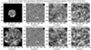 |
Fig. 1. Average images during ALMA scan 8 in Band 6 (top-left) and during scan 1 in Band 3 (bottom-left), together with the corresponding HMI magnetograms (saturated at ±50 G), as well as AIA 304 Å and Hα negative images from GONG. The insert at the top right corner of the images shows the ALMA resolution. The squares in the ALMA images show the regions analyzed for oscillations, the circles in the other images mark the ALMA field of view. All images are oriented with the celestial north pointing up. |
We note that the observed region was very quiet, so that the network (contrary to our 2017 observations) is not fully discernible in the magnetograms. Still, most peaks in the mm-wavelength images (at 3 mm in particular), are closely associated with network elements, of both positive and negative polarity. A large (∼25″ diameter) supergranular cell, centered at about x = −298″, y = −305″ (Fig. 1), covers a large part of the 1.26 cm field of view. Finally, the negative Hα images (centered at line center) from the GONG network show a strong similarity to the ALMA images, at 3 mm in particular. This is probably because GONG images are broadband; hence they are dominated by the absorption of dark mottles or spicules, which are located above network elements. We note that Molnar et al. (2019) reported a good correlation between Hα core width maps and ALMA brightness temperature at 3 mm. The average values for network and cell interior brightness temperatures for the ALMA data sets analyzed in this article are from Alissandrakis et al. (2020).
3. Analysis of oscillations
A first report on the oscillations in our April 2018 data has been presented by Jafarzadeh et al. (2021). We note, however, that these authors used pointing information for the ALMA images which was different from the one we use in this article. We selected 120 pixel × 120 pixel fields of view (FoV) around the center of each image to avoid artifacts resulting from the primary beam correction toward the edges of each FoV. Given the different pixel sizes for Band 6 and Band 3, the corresponding FoVs were 30″ × 30″ and 60″ × 60″, respectively. The selected regions are marked by the squares in the ALMA images of Fig. 1.
Since there were large interruptions between scans 4 and 5 of Band 6 observations, we did not attempt to analyze the entire time series. Instead, we split the data in two extended blocks containing scans 1−4 and 5−8, including both actual observations and gaps between scans, with a duration per block of ≈33 min. Likewise for Band 3 observations, given the large interruption between scans 3 and 4, we made two extended blocks, containing scans 1−3 and 4−6 with a total duration per block of ≈27 min. We refer to these series as Band 6 original and Band 3 original, respectively. The frequency resolution of the Band 6 and Band 3 observations for the blocks resulting from the concatenation of consecutive scans discussed above is 0.5 and 0.6 mHz, respectively.
In order to properly compare the Band 3 and Band 6 temporal variations, differences in both the beam size and the FoV for these two bands should be taken into account. Therefore, the superior spatial resolution Band 6 images were first deconvolved with the Band 6 beam, and then convolved with the Band 3 beam. This essentially yields Band 6 observations of the same spatial resolution as those of Band 3, and we thereby refer to the series from this operation as Band 6 for Band 3 beam. Next, in order to take into account the larger Band 3 FoV, we trimmed the Band 3 original FoV into a FoV which is identical to the Band 6 FoV (i.e., 30″ × 30″), and we hereby refer to results from this series as Band 3 for Band 6 FoV. Therefore, the Band 6 and Band 3 series produced from these calculations, correspond to observations with the same spatial resolution and FoV, therefore they can be subjected to meaningful comparisons.
The light curves at each pixel of the four series described above (hereafter referred to as Band 6 original, Band 3 original, Band 6 for Band 3 beam, and Band 3 for Band 6 FoV), and per given block (i.e., scans 1−4 and 5−8 for Band 6 and scans 1−3 and 4−6 for Band 3) were then submitted to Fourier transform in order to calculate the corresponding Power Spectral Density (PSD), defined as:
 (1)
(1)
where ν is the frequency, T is the duration of the time series, and P(ν) is the power spectrum of the observed light curve (Eq. (A.4)). The average value of the light curve of each individual pixel was subtracted prior to the PSD calculation and zeroes were added to fill the blanks in the concatenated light curves. Next, for each block we calculated the spatially-averaged PSD over the corresponding FoV, and finally averaged the PSD for the two blocks considered for each band. The above procedure allowed to take into account the longest possible light curves and, at the same time, to derive the most representative spectra for the entire sequence.
The resulting PSDs for the four series are displayed with the black solid lines in Fig. 2. In all cases, the p-mode peak in the vicinity of ≈3.6 − 4.4 mHz, is situated well above the spectral background. The longer duration of the present observations compared to the observations reported in Paper I (≈10 min) allowed us to better track the rollover of spectral power toward lower frequencies; it was thus not necessary to de-trend the data, as we had done in Paper I. The presence of sidelobes around the peak in all spectra is also obvious, and this is more prominent in Band 6. The introduction of gaps in our light curves introduces these sidelobes in the resulting power spectra and also influences their amplitude. In the calculations of the peak amplitudes that we are reporting throughout this paper, we corrected for the decrease in power due to the gaps. A detailed discussion of the impact of the gaps on the resulting power spectra and correction factors is given in the appendix.
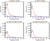 |
Fig. 2. Spatially averaged PSDs for the series discussed in Sect. 3: Band 6 original data (panel a), Band 3 original data (panel b), Band 6 data degraded to the resolution of Band 3 (panel c), and Band 6 for Band 3 FoV (panel d). The spectra of panels c and d are appropriate for meaningful comparisons between Band 6 and Band 3. Black solid lines represent the observed PSDs. Horizontal orange line corresponds to the frequency range employed in the fits. Red solid curves show the fit of the observed PSDs and red dashed lines show how the best fit extends outside the frequency range used in the fit. Solid blue lines show the absolute value of the fit residuals. |
The effect of degrading the spatial resolution of the Band 6 observations to that of the Band 3 observations is quite pronounced and leads to a significant decrease (factor ≈2 at spectral peak) of the power (compare panels a and c of Fig. 2). This is because the decrease of spatial resolution reduces the short wavelength components of the oscillations. Moreover, trimming the Band 3 FoV into the Band 6 FoV, leads to further decrease of the power by a factor of 1.4 at spectral peak (compare panels b and d of Fig. 2). This time, the reduction happens because the limitation of the FoV reduces the amplitude of the long wavelength components of the p-modes.
To proceed into a more quantitative analysis and in order to compute the total power of the chromospheric p-modes, we followed Paper I and fitted the observed PSDs with an analytical function consisting of the sum of a log-normal function (that is, Gaussian of ln(ν), ν being the frequency) and a linear function of ln(ν), which is meant to describe the p-mode (value and frequency of peak and spectral width) and the spectral background, respectively:
 (2)
(2)
where a0 − a4 correspond to the free parameters of the fitting function. The function was applied to frequency ranges of the PSDs marked with horizontal orange lines in Fig. 2 and these were deduced as follows: We first considered “search” intervals of potential lower and upper frequencies, in the 2−4 mHz and 30−50 mHz range respectively. Next, for each combination of lower and upper frequency that could be drawn from these intervals, we performed the PSD fitting and calculated the corresponding χ2. The lower and upper frequency employed in our analysis was the one leading to the smallest χ2. Experimentation showed that considering different “search” intervals, mainly for the lower frequency, led to undesirable results, since the corresponding fits were no longer able to track the spectral peaks.
In Fig. 2, we plot the PSD fits with red solid lines. Generally speaking, the employed fitting function does a decent job in reproducing the observed PSDs, as it could also be seen in the relatively small absolute residuals (blue solid lines), which do not exceed ≈20%.
From the log-normal part of the fitting function, we calculated the root-mean-square (rms) associated with the p-mode (see Eq. (3) in Paper I) while the integral of the PSD over the full spectrum, as per Parseval’s theorem, supplies the rms of the brightenss temperature, Tb, fluctuations for any temporal variation, oscillatory and non-oscillatory, of the corresponding light curves.
In Table 2, we present results from the fits of our Band 6 and Band 3 observations corresponding to the four considered series. For comparison, we also present the pertinent average values derived from the Band 3 observations of Paper I. Columns 2−8 give the p-mode rms, the ratio of p-mode rms to the average quiet Sun Tb, the rms of the full spectrum, the ratio of the full spectrum rms to the quiet Sun Tb from Alissandrakis et al. (2020), the ratio of the p-mode rms to that of the full spectrum (that is, the ratio of Cols. 3 and 5), the frequency of p-mode peak, and the full width at half maximum (FWHM) of the p-mode peak. The quoted errors represent the half value of the absolute difference of any given derived quantity between the two blocks of our observations (that is, scans 1−4 and 5−8 in Band 6 and scans 1−3 and 4−6 in Band 3). On the basis of the results presented in Table 2, we can draw the following conclusions:
Parameters of p-mode oscillations from ALMA observations at 3 and 1.26 mm from this study (rows 2−5) and from Paper I (row 1).
– The fractional p-mode rms (rms/Tb, qs), which essentially gives the relative amplitude of the p-mode, is similar (0.17−0.18) for Band 6 and Band 3.
– The original Band 6 observations, when degraded to the resolution of Band 3, exhibit a significant decrease in the rms by a factor of 1.6 which is somehow smaller than the corresponding factor in resolution (i.e., ≈2).
– Varying the employed FoV for Band 3 observations (full versus matching that of Band 6) gives rise to a difference of the rms of about 1.1.
– In both bands, the p-mode rms corresponds to a significant fraction of the full spectrum rms in the range 0.55−0.68.
– Band 3 observations of Paper I exhibit smaller p-mode rms and fractional rms with respect to the observations of this work by a factor of ≈2.1, apparently due to the inferior resolution of the data set used in Paper I.
– The frequencies of the p-mode peak lie in the range [3.6−4.4] mHz; the Band 6 peak frequencies exceed those of Band 3 but the differences are within the spectral resolution of the analyzed power spectra.
– Band 6 and Band 3 observations of this work and of Paper I exhibit FWHM in the range [3.2−3.9] mHz. The difference of FWHM in the Band 6 and 3 original time series falls within the calculated uncertainties. However, the FWHM in the “Band 3 for Band 6 FoV” time series is larger than the FWHM in the “Band 6 for Band 3 beam” time series, since their difference exceeds the relevant uncertainties.
From the p-mode rms we can make an estimate of the p-mode energy density, ϵ:
 (3)
(3)
where ρ is the mass density and δv is the velocity amplitude. For linear sound waves it is:
 (4)
(4)
where δT (equal to  times the temperature rms) is the temperature amplitude of the p-mode, T is the average temperature, cs is the sound speed and γ = 5/3.
In Eqs. (3) and (4), substituting the Band 6 fractional rms for Band 6 original data from Table 2 (this series corresponding to the highest fractional rms) and ρ from the Fontenla et al. (1993) FAL C model (corresponding to the average quiet Sun temperature in Band 6 at the disk center from Alissandrakis et al. 2020), we obtained an energy density of ≈3 × 10⁻² erg cm−3. Using observations of absorption lines formed at heights from about 130 to about 1000 km, Canfield & Musman (1973) found that the p-mode energy density decreases with height from 2 × 10² erg cm−3 at 130 km to 4 × 10⁻¹ erg cm−3 at a height of 1000 km. Alissandrakis et al. (2020) used full-disk ALMA images to detect the solar limb and derived an emission height of 2400 ± 1700 km for Band 6, which is above the heights scanned by Canfield & Musman (1973). This implies that the decreasing trend in the p-mode energy density with height extends above 1000 km.
4. Transient brightenings
4.1. Detection of transient brightenings
For our detection of transient brightenings, we followed the procedure described in Paper II. Briefly, we removed the effect of oscillations (see Sect. 3) from the light curve of each pixel. At both ALMA wavelengths, we were able to significantly suppress the oscillatory power (by factors of 13 to 16 in Band 3, and by factors of 11 to 15 in Band 6). The maximum residual oscillatory power was also similar at both wavelengths; its highest values were 42 K2 Hz−1 in Band 3 and 37 K2 Hz−1 in Band 6. These results are similar to those reported in Paper II. As in Paper II, the criteria we used for event identification were: (i) at least four consecutive points in each “corrected” time profile should have intensity exceeding a 2.5σ threshold above the mean intensity of the light curve, (ii) such behavior should also be shared by a beam-size patch of adjacent pixels (18 0.5″-pixels for Band 3 and 18 0.25″-pixels for Band 6), and (iii) the time profiles of the selected pixels should peak within ±2 min. At both frequencies the variation of the threshold parameters affects the results in manners similar to those described in Paper II.
We only used scans 1−2 and 4−5 from the Band 3 data and scans 1−3 and 5−7 from the Band 6 data, that is, we did not take into account scans 3 and 6 in Band 3 and scans 4 and 8 in Band 6 because their duration was shorter than the periods of oscillations (see Sect. 2). To compensate for the smaller field of view of the images compared to the field of view of the images used in Paper II, we submitted all of their pixels to our algorithm for the detection of transient brightenings. Pixels toward the edges of the field of view could be susceptible to artifacts introduced by the primary beam correction. However, the number of events that we detected at the outer 30-pixel ring of each field of view was rather limited (seven events in Band 3 and six events in Band 6) and their properties were indistinguishable from the properties of the rest of the events. Furthermore, it is obvious from Fig. 1 that much of the structures imaged in the ALMA images extend beyond their field of view and the problem is more serious in Band 6. To this end, we also searched for transient brightenings in the extended regions (square fields of view of 128″ × 128″ and 64″ × 64″ in Bands 3 and 6, respectively) covered by the self-calibrated CLEAN’ed images prior to the application of the primary beam correction. The possible detection of transient events beyond the circular fields of view dictated by the primary beam would increase our statistical sample, although the photometric properties of such events would not be accurate. However, we were not able to recover any more events in these areas.
We used the method described above to detect transient brightenings in 304 Å and 1600 Å AIA data (same regions and times as the ALMA images). For this task, we first convolved the AIA images with the pertinent ALMA beam. Due to the inferior cadence of the AIA images (12 s and 24 s for 304 Å and 1600 Å, respectively), we reduced the number of consecutive time profile points exceeding the 2.5σ threshold from four to one.
4.2. Properties of transient brightenings
The numbers of transient brightenings that we detected at both ALMA frequencies as well as in AIA data appear in Table 3 together with the numbers of events per unit area and time (values in parentheses). For the purposes of comparison, we also give the relevant results from Paper II. The numbers reported in Table 3 are uniformly distributed among the time intervals of the ALMA scans with the exception of the 1.26 mm events during scan 7, where only three events were identified, likely due to inferior seeing conditions.
Statistics of the 1.26 mm and 3 mm transient brightenings.
It is interesting to note that the occurrence rate per unit area of the 1.26 mm events is higher than that of the 3 mm events both from the data set presented in this article and from the data set analyzed in Paper II (factors of 2.16 and 1.07, respectively). For the proper interpretation of this result, we need to take into account the differences both in noise level and spatial resolution between the Band 3 and Band 6 data. The evaluation of noise was done using the prescription described by Shimojo et al. (2017a); see also Yokoyama et al. (2018). Briefly, in both Bands 3 and 6, ALMA receivers are equipped with systems that are sensitive to linear orthogonal polarizations; X and Y. The subtraction of simultaneous snapshot images from the XX and YY data is expected to be zero in the quiet Sun and any deviation from zero can be attributed to noise. We measured noise levels of 10.5 K and 21.2 K in Bands 3 and 6, respectively.
We also degraded the resolution of images from selected Band 6 scans to the 3 mm resolution (see also Sect. 3). The resulting images were searched for transient brightenings. We did find smaller number of events but again their occurrence rate per unit area remained higher (a factor of 1.40) than that of the Band 3 events. It appears that the very quiet area imaged in Band 6 (the interior of a supergranular cell covers much of the 1.26 mm field of view; see Sect. 2) may have helped in the identification of weak events that would otherwise have been obscured by the relatively stronger emissions in the Band 3 data. This interpretation is consistent with the higher occurrence rate per unit area of the AIA data registered with the Band 6 data than that of the AIA data registered with the Band 3 data (see Table 3).
The number of 304 Å events is higher than the number of ALMA events at a given wavelength and even more so is the number of 1600 Å events (see Table 3). As in Paper II, paired events (that is, ALMA events with AIA counterparts, either at 304 Å or 1600 Å) were identified by requesting that the ALMA and AIA events have one or more common pixels and their time profiles peak within 15 s.
The number of paired ALMA-AIA events appears in columns five and six of Table 3. As in Paper II, we did not find any event with conspicuous signatures in three wavelengths (that is, ALMA, either 1.26 mm or 3 mm, 304 Å, and 1600 Å). The percentage of 3 mm events with AIA counterparts is about 9%, which is similar to the percentage found in Paper II. On the other hand, we found no 1.26 mm events with 304 Å counterparts although 15% of the 1.26 mm events were paired with 1600 Å events. The complete absence of 304 Å counterparts to the 1.26 mm events is not a result of chance. A simple calculation reveals that the number of chance concurrences between 1.26 mm and 1600 Å events should be between less than two to more than three events.
Using the scheme presented by Nindos et al. (2018), we divided the pixels of each image into two groups: network pixels and intra-network pixels (see Alissandrakis et al. 2020 for a detailed discussion about possible pixel segregation schemes). At 3 mm, the situation is similar to that reported in Paper II, that is, there is a rather weak tendency (73%, see Table 4) for the transient brightening pixels to appear at the boundaries of the network rather than in intra-network regions. The situation is somehow different at 1.26 mm where 52% of event pixels are not located at network boundaries. This is apparent in Fig. 3 (panel a), where we have used red color to mark the pixels of the transient brightenings that occurred at 1.26 mm during scan 1. The situation in the other 1.26 mm scans is similar. Figure 3 indicates that this trend is also shared by the events detected at 1600 Å but not by those detected at 304 Å. The different trends between the 1.26 mm event locations and 3 mm event locations can be interpreted in terms of the different characteristics of the regions imaged at 1 and 3 mm; in the former, much of the field of view is occupied by the interior of a supergranular cell, which is not the case for the latter. The diversity of observed moprhologies at 1.26 mm with ALMA full-disk images has been demonstrated by Alissandrakis et al. (2017) and Brajša et al. (2018).
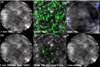 |
Fig. 3. Display (overlayed on the pertinent average images) of the pixels that were associated with transient bightenings in ALMA 1.26 mm (red), AIA 1600 Å (green), and AIA 304 Å (blue) for scan 1 data. In the images of the top row, we mark all events at each wavelength. In panels d and e of the bottom row we mark only the paired events, that is, those that were detected both at 1.26 mm and 1600 Å, respectively. Panel f: average 1.26 mm image. The white circles denote the ALMA field of view. |
Location, range of maximum intensity, area, and duration of the 1.26 mm and 3 mm transient brightenings.
We performed a statistical analysis of the event maximum intensities, durations, and areas (see Table 4 and Fig. 4). At both 1.26 mm and 3 mm, we do not report on the properties of the paired events because they were practically indistinguishable from the properties of all the events. The errors attached to the mean values were derived from the standard deviations of the corresponding parameters. The frequency distributions of the parameters we studied were all fitted with power-law functions (see Fig. 4). The uncertainties on their indices were derived from the propagation of errors associated with the histogram bins assuming Poisson statistics.
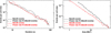 |
Fig. 4. Statistics of the duration and area of the transient brightenings. Left panel: frequency distribution of the duration of the transient brightenings detected at 1.26 mm and 3 mm (red and black solid curves, respectively). The dashed red and dashed black lines show power-law fits of those distributions. Right panel: same as left panel, but for the frequency distribution of maximum area. |
The average maximum brightness temperature of the 1.26 mm events ranged from 44 K to 449 K, while that of the 3 mm events ranged from 65 K to 511 K. The above values were measured with respect to backgrounds of ∼5540 − 6040 K and ∼7180 − 7500 K at 1.26 mm and 3 mm, respectively, after we took into account the corrections proposed by Alissandrakis et al. (2020). Therefore, at 1.26 mm we were able to detect weaker events than at 3 mm; the range of excess intensity of the latter was similar to that of the events analyzed in Paper II.
The spatial resolution of the ALMA data sets affected the mean maximum areas of the events that we measured. The superior 1.26 mm spatial resolution allowed the detection of smaller events at 1.26 mm than at 3 mm. Furthermore the average maximum size of the 3 mm events was smaller than the one reported in Paper II due to the better spatial resolution of the 2018 data. The duration of events (quantified by their FWHM) in all data sets was similar. We also note that all events were of the gradual rise and fall type (see Fig. 5 for an example), suggesting a thermal origin.
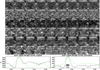 |
Fig. 5. Transient brightening detected both at 1.26 mm and 1600 Å scan 1 data. In rows (a) and (b), we show representative 1.26 mm images before and after the subtraction of the average 1.26 mm image. Rows (c), (d) and (e), (f) have the same format as rows (a) and (b) but they show the corresponding 1600 Å data and 304 Å data, respectively. The white arrows point to the transient brightening in the 1.26 mm and 1600 Å data. The field of view of all images is 20″ × 20″. In the bottom row, we present the event time profiles at 1.26 mm (black curves) and 1600 Å (green curves) before and after our processing (left and right panels, respectively). The black arrows show the times in which the 1.26 mm emission is greater than the 2.5σ threshold above average. The 1600 Å time profiles have been normalized to match the vertical range of the 1.26 mm plots. |
In Fig. 5, we show one characteristic event that was detected at both 1.26 mm and 1600 Å. Due to their weak intensity, all events at both 1.26 mm and 3 mm were not readily visible in the plain images; their visual identification was made possible after we subtracted the average image from each datacube image. In these difference images, the 3 mm events appear as unresolved bright patches while some of the 1.26 mm events are marginally resolved (for example, see the event of Fig. 5). In the same figure, the emission from the transient brightening stands out clearly from the residuals of the oscillations.
4.3. Energy budgets of transient brightenings
For the calculation of the energy budgets of the transient brightenings, we assume that they emit thermal free-free radiation, the electron density and apparent volume do not change significantly in the course of the events, and that the filling factor is unity. Then we follow the method outlined in Paper II. Briefly, the energy is proportional to: (1) The maximum excess electron temperature of a given event above background which is equal to the maximum excess brightness temperature above background because the events are optically thick; (2) The electron density which is obtained from the values of the electron densities tabulated in the Fontenla et al. (1993) FAL C model for the heights that correspond to the range of electron temperatures associated with the 1.26 mm and 3 mm emission (see also Alissandrakis et al. 2017, 2020 for details); (3) The apparent volume that is derived from the maximum area of the events (see Sect. 4.2), assuming their height is equal to their horizontal size.
The results of our computations appear in Table 5. For comparison, in the same table, we also give the results from Paper II. At 1.26 mm the energy of the transient brightenings ranges from 1.8 × 10²³ erg to 1.1 × 1026 erg while at 3 mm it ranges from 7.2 × 10²³ erg to 1.7 × 1026 erg. Therefore, at 3 mm, we derived smaller values for the lower energies of the events than in Paper II (difference of almost a factor of two), probably due to the detection of smaller and somehow weaker events (see Sect. 4.2). The same arguments apply for the interpretation of the even lower energies detected at 1.26 mm (a factor of four smaller than at 3 mm).
Energetics of the 1.26 mm and 3 mm transient brightenings.
The range of calculated energies fall within the range of values reported in previous publications that discuss quiet Sun transient brightenings. This was already mentioned in Paper II for the energies associated with the March 2017 3 mm events. The new finding here is that the low end values of the energies of the 1.26 mm events is almost one order of magnitude smaller than the presumed high-end energy limit of nanoflares (1024 erg) and among the lowest energies ever reported. Publications that have reported the detection of events with energies below 1024 erg include Aschwanden et al. (2000; 5 × 10²³ erg), Parnell & Jupp (2000; 1023 erg) and Subramanian et al. (2018; 3 × 10²³ erg).
In Fig. 6, we present the frequency distribution of both the 1.26 mm and 3 mm transient brightenings versus their energy. The gray areas in the figure denote the uncertainties in each frequency distribution which arise from the energy computations and the way we assembled each frequency distribution. If we do not take into account the low-end parts of the energies (that is, values lower than 2.7 × 10²³ erg and 1024 erg for 1.26 mm and 3 mm, respectively) we can fit the frequency distributions with power-law functions that have indices of 1.64 ± 0.04 and 1.73 ± 0.06 for the 1.26 mm and 3 mm events, respectively. Given the uncertainties involved, the derived power-law indices do not show significant differences and they are similar to the results derived for our March 2017 3 mm data, and also similar to those reported in previous publications about EUV and X-ray transient brightenings (see Paper II and references therein).
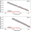 |
Fig. 6. Energetics of transient brightenings. Top panel: black curve shows the frequency distribution of the energy of the transient brightenings detected at 1.26 mm. The gray band denotes the uncertainties (see text for details). The red line shows the power-law fit, with index of 1.64, of the frequency distribution for energies higher than 2.7 × 10²³ erg. Bottom panel: same as top panel for the events detected at 3 mm. The red line shows the power-law fit, with index of 1.73, of the frequency distribution for energies higher than 1024 erg. |
In Table 5, we also give the energies per unit area and time (that is, power per unit area) of the transient brightenings which were computed after we divided the total energy of events at a given wavelength with the area of the field of view and the time intervals used for the detection of the events. A similar calculation in Paper II showed that the March 2017 3 mm transient brightenings could account for about 1% and 10% of the radiative losses in the chromosphere and corona, respectively. The 3 mm events analyzed in this article provide an almost identical result. Furthermore, it is interesting that although the occurrence rate per unit area of the 1.26 mm events is higher than that of the 3 mm events (see Sect. 4.2), their power per unit area is smaller. This result could arise from the existence of several weaker events at 1.26 mm. The combined power per unit area of transient brightenings in the two ALMA bands was found to be 0.86 × 10⁴ erg cm−2 s−1, that is, more than a factor of two smaller than that of the 3 mm events. Therefore the inclusion of weaker events enhances the divergence between the computed power per unit area and the ones required for the heating of the chromosphere and the corona.
We attempted to put the calculations of the energetics of the oscillations (see Sect. 3) on the same footing with the calculations of the energetics of the transient brightenings. To this end, we assumed that the 1.26 mm field of view was covered by beam-sized oscillating elements whose amplitude of oscillations was assumed to correspond to a brightness temperature enhancement due to a transient brightening. Then the division of the resulting energy of all oscillating elements with the period of oscillations and the area of the field of view yields a crude estimate of the power per unit area associated with the oscillations. We found that it was 18.2 × 10⁴ erg cm−2 s−1, which is a factor of 16.5 higher than the power per unit area associated with the 1.26 mm transient brightenings.
5. Conclusions and summary
Using ALMA observations of a quiet Sun region, we expanded our studies of chromospheric oscillations and transient brightenings at mm-wavelengths that were presented in Papers I and II, respectively, by including Band 6 (1.26 mm) data in our analysis. Compared to our previous publications, the data sets analyzed in this article had better spatial and temporal resolution (1 − 2″ and 1 s, respectively) as well as improved frequency resolution in spectral power (0.5 mHz), compared to 3 − 4″, 2 s, and 1.7 mHz, respectively, of our 2017 observations. As in Papers I and II, we took particular care in separating oscillations and transients from each other and from background time variations and noise.
As a result of the improved frequency resolution, the spectral peaks, in the range of about 3.6 to about 4.4 mHz, are fully visible above the background. The differences between the p-mode peak frequencies for Band 6 and Band 3 are within the spectral resolution of the analyzed power spectra. The FWHM of the p-mode peaks were found in the range [3.2,3.9] mHz. We found that short gaps in the time-series, inherent to ALMA observations, produce weak side lobes to the spectral peaks and reduce spectral power. By ignoring the side lobes and correcting the values of the spectral peak intensities, we computed the rms values of the oscillating component of the brightness temperature for the whole 120 × 120-pixel regions employed for the study of oscillations in both 1.26 mm and 3 mm.
Given the differences between the 1.26 mm and 3 mm data in terms of both spatial resolution and field of view, we also calculated: (1) the rms for the 1.26 mm data after we degraded their spatial resolution to that of 3 mm data; and (2) the rms for a trimmed 3 mm field of view equal to the 1.26 mm field of view. The rms values from these further calculations correspond to data cubes of the same field of view and spatial resolution and, hence, they were appropriate for the purpose of carrying out meaningful comparisons.
The p-mode oscillations in 1.26 mm and 3 mm exhibit small and comparable relative Tb fluctuations of ≈1.7 − 1.8% with respect to the average quiet Sun Tb corresponding to a rms of 137 and 109 K, respectively. These results imply that the p-mode relative amplitude does not appreciably change between the formation heights of the 1.26 mm and 3 mm emissions. The energy density of the p-modes in 1.26 mm is ≈3 × 10⁻² erg cm−3. The Tb fluctuations of the p-mode oscillations at 1.26 mm and 3 mm represent a significant fraction (0.55−0.68) of the total fluctuations (that is, no matter being oscillatory or not, in nature) of the light curves; since the total fluctuations include instrumental noise, the actual fraction is still higher.
The spatial resolution is affecting the rms of the p-mode oscillations in both wavelengths (we also compared the 3 mm observations of this work with those of Paper I). This implies that ALMA observations of chromospheric oscillations with a spatial resolution worse than at least 1″ are not fully resolved. We should also always bear in mind that pixels are correlated on beam scale which is around 18 pixels in both bands. This suggests that at such scales the observed oscillations are not fully independent and, therefore, some “mixing” between cell and network seems inevitable. In addition, the reduction of the full 3 mm field of view to its half, has a relatively small effect in the resulting rms (factor of ≈1.1). Taking all these effects into account, we can consider the p-mode rms of 175 K or 2.75% of the quiet Sun, measured at 1.26 mm (the 1.26 mm background brightness temperature at disk center is 6343 K; see Alissandrakis et al. 2020), as a lower limit of the actual value.
Our search for transient brightenings revealed 77 events at 1.26 mm and 115 events at 3 mm. The occurrence rate per unit area of the events that we detected is much smaller than that of the events identified by Eklund et al. (2020); these authors detected 552 events in 3 mm ALMA observations of the quiet Sun, which is equivalent of event occurrence rate per unit area almost two orders of magnitude higher than those found in both the present study and in Paper II. One possible explanation of this discrepancy is that the quiet Sun region that Eklund et al. (2020) observed was very different from the one we did. On the other hand, it is not clear in their article that they removed the oscillations, thus some oscillation peaks may have been mistaken as transients.
The occurrence rate per unit area of our 1.26 mm events was higher than that of the 3 mm events. This conclusion does not change even if we take into account differences in noise levels and spatial resolution between the two data sets (although there is a decrease of the relevant factor from 2.16 to 1.4). Much of the field of view of the 1.26 mm observations is covered by the interior of a supergranular cell and the absence of strong background sources may have contributed to the detection of weak events that could otherwise have been missed.
The predominance of cell pixels in the 1.26 mm field of view may also explain the slight preference of the 1.26 mm events to occur in cell regions – in contrast to the opposite trend that was exhibited by the 3 mm events. We note that there is a long history of detection of transient brightenings in intranetwork regions that dates back to the publication of such an event by Nindos et al. (1999) to the more recent reports about the multitude of events associated with the cancellation of intranetwork magnetic fields (Gošić et al. 2018). Another distinct property of the 1.26 mm events was that they had no 304 Å counterparts although 15% of them were paired with 1600 Å events. Presumably the 1.26 mm events are located at much deeper and cooler layers of the solar atmosphere than the 304 Å events and their strength may not be sufficient to give rise to 304 Å emission.
At both wavelengths all transient brightenings show time profiles with a gradual rise and fall and durations of about 50 s. Furthermore, at both wavelengths we were able to detect events with sizes down to the size of the instrumental spatial resolution. At 1.26 mm we detected events that were somehow weaker than the 3 mm events (excess brightness temperatures of 44−449 and 65−511 K above background, respectively). The intensity and duration of the transient brightenings is not consistent with the relevant observed properties of the events discussed by Eklund et al. (2020) who attributed them to shock waves.
The energies supplied by the transient brightenings were in the ranges of 1.8 × 10²³ to 1.1 × 1026 erg and 7.2 × 10²³ to 1.7 × 1026 erg for the 1.26 mm and 3 mm events, respectively. The power-law indices of the frequency distributions of the events were similar (1.64 and 1.73 for the 1.26 mm and 3 mm, respectively) and close to the one reported in Paper II. At 3 mm the lower end of the energies falls below that of the events of Paper II possibly due to the detection of events with smaller sizes. Even lower was the lower end of the energy distribution of the 1.26 mm events, which is among the smallest ever reported in the literature of transient brightenings irrespective of the wavelength of observations. Although the occurrence rate per unit area of the 1.26 mm events is higher, their power per unit area is smaller than that of the 3 mm events probably due to the detection of many weak 1.26 mm events.
We also found that broadband Hα negative images show a strong similarity to the ALMA images; this is probably because broadband Hα images are dominated by the absorption of dark mottles, spicules, or fibrils, which are located above network elements observed by ALMA; for more details, see Rutten (2017) and Martínez-Sykora et al. (2020). We also note that Molnar et al. (2019) found a good correlation between maps of Hα core width and ALMA brightness temperature at 3.0 mm.
It is widely known that the quiet choromspheric emission shows significant time variation. Our study demonstrates that most fluctuations at 1.26 and 3 mm are related to p-mode oscillations since they are ubiquitous and provide more than ∼60% of the total fluctuations. The removal of oscillations from the data revealed several transient brightenings. The combined power per unit area of the transients in the two ALMA bands was about 230 times smaller than the chromospheric radiative losses. Although with the inclusion of the 1.26 mm events the minimum observed energy was pushed to values as low as about 2 × 10²³ erg, the amount of missing power per unit area increased due to the occurrence of several weaker events at 1.26 mm.
More comprehensive results both on oscillations and on the height distribution of the occurrence rate per unit area of the transient brightenings could be reached if: (1) snapshot images at different spectral windows within the same ALMA band are analyzed (in our study, data from all spectral windows of a given band were summed over); and (2) observations at a broader range of ALMA bands become available. Since late 2019, Band 7 (0.85 mm) solar ALMA observations have become available and future plans include the usage of Band 5 (1.4 mm) by the end of 2021. Furthermore, future studies of both oscillations and transient brightenings will benefit significantly from the availability of data obtained with higher spatial resolution resulting from a possible future expansion of ALMA’s long baselines.
Acknowledgments
The authors wish to thank Rob Rutten for interesting discussions on the association of ALMA emission and Hα. This work makes use of the following ALMA data: ADS/JAO.ALMA2017.1.00653.S. ALMA is a partnership of ESO (representing its member states), NSF (USA) and NINS (Japan), together with NRC (Canada) and NSC and ASIAA (Taiwan), and KASI (Republic of Korea), in cooperation with the Republic of Chile. The Joint ALMA Observatory is operated by ESO, AUI/NRAO and NAOJ. The use of SDO and GONG data from the respective data bases is gratefully acknowledged.
References
- Alissandrakis, C. E., Patsourakos, S., Nindos, A., & Bastian, T. S. 2017, A&A, 605, A78 [NASA ADS] [CrossRef] [EDP Sciences] [Google Scholar]
- Alissandrakis, C. E., Nindos, A., Bastian, T. S., et al. 2020, A&A, 640, A57 [NASA ADS] [CrossRef] [EDP Sciences] [Google Scholar]
- Aschwanden, M. J., Tarbell, T. D., Nightingale, R. W., et al. 2000, ApJ, 535, 1047 [NASA ADS] [CrossRef] [Google Scholar]
- Bastian, T. S., Chintzoglou, G., De Pontieu, B., et al. 2017, ApJ, 845, L19 [NASA ADS] [CrossRef] [Google Scholar]
- Bracewell, R. 1965, McGraw-Hill Electrical and Electronic Engineering Series (New York: McGraw-Hill) [Google Scholar]
- Brajša, R., Sudar, D., Benz, A. O., et al. 2018, A&A, 613, A17 [NASA ADS] [CrossRef] [EDP Sciences] [Google Scholar]
- Canfield, R. C., & Musman, S. 1973, ApJ, 184, L131 [Google Scholar]
- Carlsson, M., De Pontieu, B., & Hansteen, V. H. 2019, ARA&A, 57, 189 [NASA ADS] [CrossRef] [Google Scholar]
- da Silva Santos, J. M., de la Cruz Rodríguez, J., White, S. M., et al. 2020, A&A, 643, A41 [EDP Sciences] [Google Scholar]
- de Wijn, A. G., McIntosh, S. W., & De Pontieu, B. 2009, ApJ, 702, L168 [NASA ADS] [CrossRef] [Google Scholar]
- Eklund, H., Wedemeyer, S., Szydlarski, M., et al. 2020, A&A, 644, A152 [NASA ADS] [CrossRef] [EDP Sciences] [Google Scholar]
- Eklund, H., Wedemeyer, S., Snow, B., et al. 2021, Philos. Trans. R. Soc. London Ser. A, 379, 20200185 [NASA ADS] [Google Scholar]
- Fontenla, J. M., Avrett, E. H., & Loeser, R. 1993, ApJ, 406, 319 [Google Scholar]
- Gošić, M., de la Cruz Rodríguez, J., De Pontieu, B., et al. 2018, ApJ, 857, 48 [NASA ADS] [CrossRef] [Google Scholar]
- Guevara Gómez, J. C., Jafarzadeh, S., Wedemeyer, S., et al. 2021, Philos. Trans. R. Soc. London Ser. A, 379, 20200184 [Google Scholar]
- Henriques, V. M. J., Kuridze, D., Mathioudakis, M., & Keenan, F. P. 2016, ApJ, 820, 124 [NASA ADS] [CrossRef] [Google Scholar]
- Jafarzadeh, S., Wedemeyer, S., Szydlarski, M., et al. 2019, A&A, 622, A150 [NASA ADS] [CrossRef] [EDP Sciences] [Google Scholar]
- Jafarzadeh, S., Wedemeyer, S., Fleck, B., et al. 2021, Philos. Trans. R. Soc. London Ser. A, 379, 20200174 [NASA ADS] [Google Scholar]
- Jess, D. B., Morton, R. J., Verth, G., et al. 2015, Space Sci. Rev., 190, 103 [Google Scholar]
- Lemen, J. R., Title, A. M., Akin, D. J., et al. 2012, Sol. Phys., 275, 17 [Google Scholar]
- Loukitcheva, M. 2019, Adv. Space Res., 63, 1396 [Google Scholar]
- Loukitcheva, M., Solanki, S. K., & White, S. 2006, A&A, 456, 713 [NASA ADS] [CrossRef] [EDP Sciences] [Google Scholar]
- Loukitcheva, M. A., White, S. M., & Solanki, S. K. 2019, ApJ, 877, L26 [Google Scholar]
- Martínez-Sykora, J., De Pontieu, B., de la Cruz Rodríguez, J., et al. 2020, ApJ, 891, L8 [CrossRef] [Google Scholar]
- Molnar, M. E., Reardon, K. P., Chai, Y., et al. 2019, ApJ, 881, 99 [NASA ADS] [CrossRef] [Google Scholar]
- Nindos, A., Kundu, M. R., & White, S. M. 1999, ApJ, 513, 983 [Google Scholar]
- Nindos, A., Alissandrakis, C. E., Bastian, T. S., et al. 2018, A&A, 619, L6 [NASA ADS] [CrossRef] [EDP Sciences] [Google Scholar]
- Nindos, A., Alissandrakis, C. E., Patsourakos, S., et al. 2020, A&A, 638, A62 [EDP Sciences] [Google Scholar]
- Parnell, C. E., & Jupp, P. E. 2000, ApJ, 529, 554 [NASA ADS] [CrossRef] [Google Scholar]
- Patsourakos, S., Alissandrakis, C. E., Nindos, A., et al. 2020, A&A, 634, A86 [NASA ADS] [CrossRef] [EDP Sciences] [Google Scholar]
- Rutten, R. J. 2017, A&A, 598, A89 [NASA ADS] [CrossRef] [EDP Sciences] [Google Scholar]
- Schmieder, B. 2007, AIP Conf. Proc., 895, 49 [Google Scholar]
- Shibasaki, K., Alissandrakis, C. E., & Pohjolainen, S. 2011, Sol. Phys., 273, 309 [Google Scholar]
- Shimizu, T. 2015, Phys. Plasmas, 22, 101207 [Google Scholar]
- Shimojo, M., Bastian, T. S., Hales, A. S., et al. 2017a, Sol. Phys., 292, 87 [Google Scholar]
- Shimojo, M., Hudson, H. S., White, S. M., et al. 2017b, ApJ, 841, L5 [NASA ADS] [CrossRef] [Google Scholar]
- Shimojo, M., Kawate, T., Okamoto, T. J., et al. 2020, ApJ, 888, L28 [Google Scholar]
- Subramanian, S., Kashyap, V. L., Tripathi, D., et al. 2018, A&A, 615, A47 [CrossRef] [EDP Sciences] [Google Scholar]
- Tsiropoula, G., Tziotziou, K., Kontogiannis, I., et al. 2012, Space Sci. Rev., 169, 181 [NASA ADS] [CrossRef] [Google Scholar]
- Wedemeyer-Böhm, S., Lagg, A., & Nordlund, Å. 2009, Space Sci. Rev., 144, 317 [NASA ADS] [CrossRef] [Google Scholar]
- Wedemeyer, S., Bastian, T., Brajša, R., et al. 2016, Space Sci. Rev., 200, 1 [NASA ADS] [CrossRef] [Google Scholar]
- Wedemeyer, S., Szydlarski, M., Jafarzadeh, S., et al. 2020, A&A, 635, A71 [CrossRef] [EDP Sciences] [Google Scholar]
- White, S. M., Loukitcheva, M., & Solanki, S. K. 2006, A&A, 456, 697 [NASA ADS] [CrossRef] [EDP Sciences] [Google Scholar]
- Yokoyama, T., Shimojo, M., Okamoto, T. J., et al. 2018, ApJ, 863, 96 [NASA ADS] [CrossRef] [Google Scholar]
Appendix A: Effect of data gaps
The observed time series, f(t), can be described as the product of the original (infinite) time series, f0(t) and a window function, W(t),
 (A.1)
(A.1)
In our case the window function is the sum of Π functions, each of width Δti (the duration of each scan) and shifted by δti with respect to the start of the first scan:
 (A.2)
(A.2)
where n is the number of scans in a block (four for Band 6 and three for Band 3) and Π is the well-known widow function:
 (A.3)
(A.3)
The observed power spectrum, P(ν), is the square of the modulus of the Fourier Transform (FT) of the observed time series:
 (A.4)
(A.4)
where ν is the frequency and ∼ symbolizes the FT:
 (A.5)
(A.5)
Using the similarity, shift and convolution theorems of FT (see, e.g., Bracewell 1965), we obtain from (A.1) and (A.2):
 (A.6)
(A.6)
where * denotes convolution and the sinc function (FT of Π(t)) is defined as:
 (A.7)
(A.7)
The power spectrum cannot be computed analytically from (A.6), unless f0(t) is specified, because it involves the module of a convolution. For the sake of illustration, let us compute the spectrum for a monochromatic oscillation of frequency ν0, whose FT is:
 (A.8)
(A.8)
with δ being the Dirac delta function. In this case, substituting (A.6) to (A.4), we obtain:
![Mathematical equation: $$ \begin{aligned} P(\nu )=\left|\sum _{j=1}^n \mathrm{e}^{-2\pi i \delta t_j (\nu -\nu _0)} \Delta t_j\,\mathrm{sinc} [\Delta t_j (\nu -\nu _0)]\right|^2. \end{aligned} $$](/articles/aa/full_html/2021/08/aa41241-21/aa41241-21-eq14.gif) (A.9)
(A.9)
An indication of the effect of gaps can be provided by the summation term in the right-hand side of (A.6), the modulus of which is plotted in the top panel of Fig. A.1 (black line), together with that for a data set without gaps (red line). Due to the limited total duration of the observation, both data sets show side lobes; the gaps produce extra side lobes, the strongest of which reach about 25% of the peak intensity. The side lobe effect is smaller (below 10%) in the monochromatic power spectra, plotted in the bottom panel of the figure.
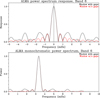 |
Fig. A.1. Effect of gaps. Top panel: modulus of the summation term in (A.6) for our Band 6 observations. The power spectrum of a monochromatic oscillation at 3.333 mHz is plotted in the bottom panel. The red curve is for a 30 min observation without gaps, the black curve is for an observation with the gaps of our Band 6 data set. All plots are normalized to a peak value of unity. |
We note that in both cases the width of the main peak is practically unaffected by the gaps. However, the value of the peak power in the presence of gaps is reduced, since, from (A.9):
 (A.10)
where Δtf is the total duration of the time series and Δtg is the duration of the gaps; thus the peak power in the series with gaps is reduced by a factor of:
 (A.11)
with respect to the peak of the time series without gaps. In our case this factor amounts to 0.6 for Band 6 and 0.7 for Band 3.
All Tables
Parameters of p-mode oscillations from ALMA observations at 3 and 1.26 mm from this study (rows 2−5) and from Paper I (row 1).
Location, range of maximum intensity, area, and duration of the 1.26 mm and 3 mm transient brightenings.
All Figures
|
Fig. 1. Average images during ALMA scan 8 in Band 6 (top-left) and during scan 1 in Band 3 (bottom-left), together with the corresponding HMI magnetograms (saturated at ±50 G), as well as AIA 304 Å and Hα negative images from GONG. The insert at the top right corner of the images shows the ALMA resolution. The squares in the ALMA images show the regions analyzed for oscillations, the circles in the other images mark the ALMA field of view. All images are oriented with the celestial north pointing up. |
| In the text | |
|
Fig. 2. Spatially averaged PSDs for the series discussed in Sect. 3: Band 6 original data (panel a), Band 3 original data (panel b), Band 6 data degraded to the resolution of Band 3 (panel c), and Band 6 for Band 3 FoV (panel d). The spectra of panels c and d are appropriate for meaningful comparisons between Band 6 and Band 3. Black solid lines represent the observed PSDs. Horizontal orange line corresponds to the frequency range employed in the fits. Red solid curves show the fit of the observed PSDs and red dashed lines show how the best fit extends outside the frequency range used in the fit. Solid blue lines show the absolute value of the fit residuals. |
| In the text | |
|
Fig. 3. Display (overlayed on the pertinent average images) of the pixels that were associated with transient bightenings in ALMA 1.26 mm (red), AIA 1600 Å (green), and AIA 304 Å (blue) for scan 1 data. In the images of the top row, we mark all events at each wavelength. In panels d and e of the bottom row we mark only the paired events, that is, those that were detected both at 1.26 mm and 1600 Å, respectively. Panel f: average 1.26 mm image. The white circles denote the ALMA field of view. |
| In the text | |
|
Fig. 4. Statistics of the duration and area of the transient brightenings. Left panel: frequency distribution of the duration of the transient brightenings detected at 1.26 mm and 3 mm (red and black solid curves, respectively). The dashed red and dashed black lines show power-law fits of those distributions. Right panel: same as left panel, but for the frequency distribution of maximum area. |
| In the text | |
|
Fig. 5. Transient brightening detected both at 1.26 mm and 1600 Å scan 1 data. In rows (a) and (b), we show representative 1.26 mm images before and after the subtraction of the average 1.26 mm image. Rows (c), (d) and (e), (f) have the same format as rows (a) and (b) but they show the corresponding 1600 Å data and 304 Å data, respectively. The white arrows point to the transient brightening in the 1.26 mm and 1600 Å data. The field of view of all images is 20″ × 20″. In the bottom row, we present the event time profiles at 1.26 mm (black curves) and 1600 Å (green curves) before and after our processing (left and right panels, respectively). The black arrows show the times in which the 1.26 mm emission is greater than the 2.5σ threshold above average. The 1600 Å time profiles have been normalized to match the vertical range of the 1.26 mm plots. |
| In the text | |
|
Fig. 6. Energetics of transient brightenings. Top panel: black curve shows the frequency distribution of the energy of the transient brightenings detected at 1.26 mm. The gray band denotes the uncertainties (see text for details). The red line shows the power-law fit, with index of 1.64, of the frequency distribution for energies higher than 2.7 × 10²³ erg. Bottom panel: same as top panel for the events detected at 3 mm. The red line shows the power-law fit, with index of 1.73, of the frequency distribution for energies higher than 1024 erg. |
| In the text | |
|
Fig. A.1. Effect of gaps. Top panel: modulus of the summation term in (A.6) for our Band 6 observations. The power spectrum of a monochromatic oscillation at 3.333 mHz is plotted in the bottom panel. The red curve is for a 30 min observation without gaps, the black curve is for an observation with the gaps of our Band 6 data set. All plots are normalized to a peak value of unity. |
| In the text | |
Current usage metrics show cumulative count of Article Views (full-text article views including HTML views, PDF and ePub downloads, according to the available data) and Abstracts Views on Vision4Press platform.
Data correspond to usage on the plateform after 2015. The current usage metrics is available 48-96 hours after online publication and is updated daily on week days.
Initial download of the metrics may take a while.