| Issue |
A&A
Volume 652, August 2021
|
|
|---|---|---|
| Article Number | A115 | |
| Number of page(s) | 10 | |
| Section | Stellar structure and evolution | |
| DOI | https://doi.org/10.1051/0004-6361/202141218 | |
| Published online | 20 August 2021 | |
Nebular Hα emission in Type Ia supernova 2016jae
1
INAF – Osservatorio Astronomico di Padova, vicolo dell’Osservatorio 5, Padova 35122, Italy
e-mail: This email address is being protected from spambots. You need JavaScript enabled to view it.
2
Institute of Space Sciences (ICE, CSIC), Campus UAB, Carrer de Can Magrans s/n, 08193 Barcelona, Spain
3
Kavli Institute for Astronomy and Astrophysics, Peking University, Yi He Yuan Road 5, Hai Dian District, Beijing 100871, PR China
4
Núcleo de Astronomía de la Facultad de Ingeniería y Ciencias, Universidad Diego Portales, Av. Ejéercito 441, Santiago, Chile
5
Millennium Institute of Astrophysics, Santiago, Chile
6
Observatories of the Carnegie Institution for Science, 813 Santa Barbara Street, Pasadena, CA 91101, USA
7
Las Campanas Observatory, Carnegie Observatories, Casilla 601, La Serena, Chile
Received:
30
April
2021
Accepted:
28
June
2021
Abstract
There is a wide consensus that Type Ia supernovae (SNe Ia) originate from the thermonuclear explosion of CO white dwarfs (WDs), with the lack of hydrogen in the observed spectra as a distinctive feature. Here, we present supernova (SN) 2016jae, which was classified as an SN Ia from a spectrum obtained soon after its discovery. The SN reached a B-band peak of −17.93 ± 0.34 mag, followed by a fast luminosity decline with sBV0.56 ± 0.06 and inferred Δm15(B) of 1.88 ± 0.10 mag. Overall, the SN appears to be a ‘transitional’ event between a ‘normal’ SN Ia and a very dim SN Ia, such as 91bg-like SNe. Its peculiarity is that two late-time spectra, taken at +84 and +142 days after the peak, show a narrow line of Hα (with full width at half maximum of ∼650 and 1000 km s−1, respectively). This is the third low-luminosity and fast-declining SN Ia, after SN2018cqj/ATLAS18qtd and SN2018fhw/ASASSN-18tb, found in the 100IAS survey to show a resolved narrow Hα line in emission in its nebular-phase spectra. We argue that the nebular Hα emission originates in an expanding hydrogen-rich shell (with velocity ≤1000 km s−1). The hydrogen shell velocity is too high to be produced during a common envelope phase, though it may be consistent with some material stripped from an H-rich companion star in a single-degenerate progenitor system. However, the derived mass of this stripped hydrogen is ∼0.002–0.003 M⊙, which is much less than that expected (> 0.1 M⊙) from standard models for these scenarios. Another plausible sequence of events is a weak SN ejecta interaction with an H shell ejected by optically thick winds or a nova-like eruption on the CO WD progenitor some years before the SN explosion.
Key words: supernovae: general / supernovae: individual: SN2016jae / supernovae: individual: SN2018cqj / supernovae: individual: SN 2018fhw
© ESO 2021
1. Introduction
Type Ia supernovae (SNe Ia) are believed to originate from the thermonuclear explosion of CO white dwarfs (WDs). In a popular explosion scenario, the WD is in a close binary system with another WD (double-degenerate system) or with a non-degenerate mass-donor companion, either a main-sequence star or a giant star (single-degenerate system). In the merging scenario the combined mass of the WDs may meet or exceed the Chandrasekhar limit (∼1.4 M⊙), while in the single-degenerate scenario the mass transfer from the secondary star makes the primary WD approach the Chandrasekhar limit. In both cases, the final fate of the system is the explosion. There are also alternative scenarios in which the explosion occurs without reaching the Chandrasekhar mass (i.e., a sub-Chandrasekhar-mass explosion). Which is the dominant scenario is still unknown (see e.g., Maoz et al. 2014). A distinctive feature of SNe Ia is the lack of hydrogen in the observed spectra. Yet, at least for single-degenerate systems, it is expected that some H from the main-sequence companion star is left in the system. In fact, finding H in SNe Ia would strongly support the single-degenerate scenario. Several attempts have been made to detect H in SNe Ia, but no convincing evidence has been found yet (e.g., Mattila et al. 2005; Tucker et al. 2020). Hydrogen has so far only been found in SN Ia-circumstellar material (CSM) events, where narrow H emissions have been present since early phases1 and are probably excited in the shock between the supernova (SN) ejecta and H-rich CSM (e.g., Hamuy et al. 2003; Prieto et al. 2007; Dilday et al. 2012; Silverman et al. 2013; consider also Benetti et al. 2006 for an alternative interpretation).
Recently, two cases of low-luminosity SNe Ia with detection of narrow Hα emission lines in late-time spectra have been reported: SN 2018fhw/ASASSN-18tb (Kollmeier et al. 2019; Vallely et al. 2019) and SN 2018cqj/ATLAS18qtd (Prieto et al. 2020). These two SNe were followed as part of the 100IAS survey (Dong et al. 2018), a project aiming at collecting a homogeneous sample of ∼100 SNe Ia with optical nebular-phase spectra using 5–10 m class telescopes. Both SNe show strong emission lines of Hα at phases > 100 d, with luminosities in the range of ∼1036–1038 erg s−1 (Hα emission lines in SNe Ia-CSM can reach luminosities in the range 1040–1041 erg s−1; Silverman et al. 2013).
Here we report a third case, SN 2016jae (α = 09h 42m 34 49, δ = +10° 59′ 35
 7; J2000.0), also known as ATLAS16eay, MASTER OT J094234.49+105935.7, CSS170201-094234+105935, Gaia16cev, and PS16fkf. It was discovered on 2016 December 21.99 UT, with an unfiltered magnitude of 17.2, by the MASTER Global Robotic Net (Gress et al. 2016)2. Independent discoveries were also reported by the Asteroid Terrestrial-impact Last Alert System (ATLAS; Tonry et al. 2016, 2018; Smith et al. 2020), the Gaia transient survey (Hodgkin et al. 2013), and Pan-STARRS (Chambers et al. 2016; Magnier et al. 2020). It was classified on 2016 December 28.34 UT (Smith et al. 2016a,b) as an SN Ia approximately one week post-maximum by the Public ESO (European Southern Observatory) Spectroscopic Survey for Transient Objects (PESSTO; Smartt et al. 2015).
In the next section (Sect. 2), we describe the host environment of SN 2016jae. Photometric and spectroscopic data are analysed in Sect. 3, and the discussion is in Sect. 4.
2. Host environment
The galaxy in the closest angular separation with SN 2016jae is SDSS J094234.46+105931.1 (hereafter SDSS-SW), a tiny galaxy located at 4 2 S, 0
 6 W from the SN (see Fig. 1). The candidate host galaxy has a magnitude in r of 21.67 and a photometric redshift of 0.35 ± 0.08 according to the Sloan Digital Sky Survey (SDSS) Data Release (DR) 15 catalogue3. However, the redshift derived from the spectrum of SN 2016jae using the Supernova Identification (SNID) cross-correlation code (Blondin & Tonry 2007), z = 0.021 ± 0.006, is not consistent with the redshift of that galaxy.
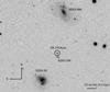 |
Fig. 1. Dark Energy Camera Legacy Survey (DECals) DR7 r deep image of the SN 2016jae field. The SN and the three nearby galaxies discussed in the text (SDSS-SW, SDSS-SE, and SDSS-NW) are indicated. We consider DL = 92.9 ± 4.3 Mpc to estimate the physical projected distance in the scale bar. We argue that SN 2016jae most likely exploded in the outer halo of SDSS-SE, as this is the nearest galaxy with a similar redshift. |
There are other two galaxies in the proximity of SN 2016jae, SDSS J094235.65+105905.3 (hereafter SDSS-SE) and SDSS J094234.01+110022.8 (hereafter SDSS-NW), which are located at 30 0 S, 17
 3 E and 47
 5 N, 7
 3 W, respectively, from the SN. We took a spectrum of SDSS-SW and SDSS-SE with the 10 m Gran Telescopio Canarias (GTC) on 2019 December 3 and another spectrum of SDSS-SW and SDSS-NW, again with the GTC, on 2020 May 10. Both spectra were reduced as described in Sect. 3.2. In the case of SDSS-SW, we combined the spectra of different epochs to improve the signal-to-noise ratio (see Fig. A.1). Comparing the spectrum of SDSS-SW with a template spectrum of a late-type galaxy (from the Kinney-Calzetti Spectral Atlas; Calzetti et al. 1994; Kinney et al. 1996) and measuring the position of Hα, Hβ, [O II], and [O III] emission lines, we found that SDSS-SW is consistent with being a background galaxy at z = 0.285 ± 0.009 (similar to the SDSS photometric redshift). Measuring the position of the same emission lines, plus [N II] and [S II] in the SDSS-SE spectrum and Hα, [O III], and [S II] in SDSS-NW, we derive redshifts of 0.021 ± 0.001 and 0.019 ± 0.001, respectively, which are consistent with the redshift of the SN derived from fitting its near-peak spectrum. This suggests that SN 2016jae exploded in the outer halo of one of these galaxies, most likely in the closest one, SDSS-SE. Throughout the paper, we adopt the zhost = 0.021 of SDSS-SE as the reference redshift. However, we cannot rule out that the SN is actually located in the halo of SDSS-NW. The implication of assuming zhost = 0.019 is discussed in Sect. 4. From the adopted redshift we derived a luminosity distance of 92.9 ± 4.3 Mpc4 (m − M = 34.8 ± 0.1 mag), assuming a Hubble constant H0 = 67.8 km s−1 Mpc, Ωm = 0.31, and ΩΛ = 0.69 (Planck Collaboration XIII 2016). With this distance, the projected linear offset from the SDSS-SE nucleus is 15.6 kpc.
The Milky Way extinction along the line of sight of the SN is AV,MW = 0.051 mag (NED5; Schlafly & Finkbeiner 2011). There is no evidence of narrow Na ID absorption in the spectra, which would have indicated the presence of gas and dust along the line of sight. Taking advantage of the fact that SNe Ia are known for their ‘homogeneity’, we considered different methods for estimating the extinction (AV) towards SN 2016jae based on comparisons of the object’s spectral energy distribution (SED) and luminosity with those of other similar SNe Ia. As we discuss in the next section, SN 2016jae is a transitional event between ‘normal’ SNe Ia and sub-luminous SNe Ia, such as SN 1991bg. Then, we matched the intrinsic (B − V)0 and (r − i)0 colour curves of SN 2016jae with those of SN 2018cqj (Prieto et al. 2020) and SN 2018fhw (Vallely et al. 2019), both of which have a similar decline rate, and that of SN 1991bg, the prototype of sub-luminous SNe Ia (Filippenko et al. 1992; Leibundgut et al. 1993; Turatto et al. 1996); we obtained E(B − V)V, tot = 0.09 ± 0.03 mag (see Fig. A.2). For comparison, we also show the colour curves of the normal SNe Ia 1992A (Kirshner et al. 1993) and 2011fe (Pereira et al. 2013). Additionally, we contrasted the early-time optical SED of SN 2016jae with those of 91bg-like SNe Ia at similar epoch. The SED of the reference SNe were first corrected for redshift and Galactic extinction. From this comparison a colour excess of E(B − V)V, host = 0.09 ± 0.01 mag was derived. We adopted E(B − V) = 0.10 ± 0.03 mag (i.e., AV = 0.30 ± 0.10 mag) as the total extinction towards SN 2016jae.
3. Data and analysis
3.1. Photometry
We used BVri photometry of SN 2016jae between 2016 December 28 (close to its peak magnitude) and 2017 February 13 from the CNIa0.02 programme6 (Chen et al. 2020) and taken with the 1 m telescopes of the Las Cumbres Observatory Global Telescope (LCOGT) network (Brown et al. 2013). We also retrieved three epochs of Gaia-band photometry from the Gaia transient survey7 and a late-time (phase 142d) r-band photometric measurement of SN 2016jae with the 10.4 m GTC and the Optical System for Imaging and low-Intermediate-Resolution Integrated Spectroscopy (OSIRIS) at the Roque de los Muchachos Observatory (Spain). The Gaia data were converted to r-band magnitude using the relationships reported in Gaia DR2 documentation (release 1.2)8. The GTC SN magnitudes were measured using point-spread-function (PSF) fitting with the SNOoPy9 pipeline. We calibrated the instrumental magnitudes to standard photometric systems using the zero points and colour terms measured through reference SDSS stars in the field of SN 2016jae. We present the final calibrated photometry of SN 2016jae in Table C.1.
The BVri light curves of SN 2016jae are shown in the left panel of Fig. 2. The data are relative to the B maximum date that occurred on 2016 December 28.2, or modified Julian date (MJD) 57750.2 ± 1.0. It was obtained by matching the light curve peak with the SNOOPY fitting package (Burns et al. 2011) using the colour stretch parameter sBV models. Allowing for the poor sampling around the maximum light, we obtained the following fits: Bmax = 17.32 ± 0.11 mag, Vmax = 16.77 ± 0.07 mag, rmax = 16.78 ± 0.07 mag, imax = 17.07 ± 0.08 mag, and sBV = 0.56 ± 0.06. The light curves of SN 2016jae have a good sampling after maximum light up to +42 d later, showing in all bands a fast decline until the radioactive decay at t ∼20 d in the B band. This decay translates to Δm15(B) of 1.88 ± 0.10 mag using the sBV–Δm15 relationship in Burns et al. (2018). Based on the light curves, SN 2016jae qualifies as an intermediate case between normal and sub-luminous and fast-declining SNe Ia. In fact: (i) The Δm15 of SN 2016jae is between that typical for normal SNe Ia, ≲1.7 mag, and that of 91bg-like SNe, 1.8–2.1 mag (see e.g., Taubenberger et al. 2017). (ii) The B absolute magnitude peak of SN 2016jae is −17.93 ± 0.34, dimmer than normal SNe Ia such as SNe 1992A and 2011fe (see Fig. 2, right panel) and similar to other fast-decliner objects such as SNe 2018cqj and 2018fhw. We note that these last two SNe are more luminous than SN 1991bg, as illustrated in Fig. 2. Indeed, the location of SN 2016jae in the figure MBmax versus (Bmax − Vmax) colour (Fig. 7 of Phillips 2012) falls rather close to transitional SNe such as 86G-like ones (see Fig. A.3). (iii) The ‘pseudo-bolometric’ (integrating the flux in the BVri bands) peak luminosity of SN 2016jae, log(L) = 42.49 ± 0.07, is consistent with those of other sub-luminous SNe Ia. (iv) Unlike a 91bg-like SN, the light curve in the i band shows a flattening at ∼20 days, though not a secondary peak as typically seen in the redder light curves of normal SNe Ia. According to Kasen (2006) and Blondin et al. (2015), the secondary near-infrared peak in SNe Ia is related to a recombination wave propagating through chemically stratified ejecta. Consequently, the recombination of Fe III to Fe II would occur earlier in less luminous and cooler SNe. (v) We can estimate the mass of 56Ni synthesized in an explosion through the bolometric peak (Stritzinger & Leibundgut 2005). We derived a lower limit (because we only integrated the flux in the BVri bands) for the 56Ni mass of 0.15 M⊙ for SN 2016jae. Similar masses have also been estimated for SNe 2018cqj and 2018fhw10 (computed in a similar manner). This is marginally larger than the range found for the 91bg-like SNe (between 0.05 and 0.10 M⊙; Taubenberger et al. 2017).
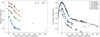 |
Fig. 2. Optical broadband light curves of SN 2016jae. Left: BVri light curves of SN 2016jae. The light curves have been shifted for clarity by the amounts indicated in the legend. Right: absolute B light curve of SN 2016jae, shown along with those of SNe 1991bg, 2018cqj, 2018fhw, 1992A, and 2011fe. For both panels, the dot-dashed vertical line indicates the B-band maximum light. The uncertainties for most data points are smaller than the plotted symbols. |
3.2. Spectroscopy
We analysed three optical spectra of SN 2016jae (see Table C.2 for basic information on the spectroscopic observations). The first spectrum was taken for the transient classification at the 3.6 m New Technology Telescope (NTT) on 2016 December 28.34 by the international collaboration PESSTO11. Two more spectra were obtained at nebular phase, on 2017 March 22.19 and 2017 May 18.91, with the Magellan Clay telescope (as part of 100IAS) at Las Campanas Observatory and with the GTC at Roque de los Muchachos Observatory, respectively. All the spectra were obtained with the slit aligned with the parallactic angle to minimize differential flux losses caused by atmospheric refraction.
All spectra were reduced following standard procedures with IRAF routines. The two-dimensional frames were corrected by bias and flat field before the extraction of the one-dimensional spectra. We wavelength-calibrated the spectra via comparison with arc-lamp spectra. The flux calibration was done using spectrophotometric standard stars, which also helped in removing the strongest telluric absorption bands present in the spectra (in some cases, residuals are still present after the correction). The wavelength calibration was verified against the bright night-sky emission lines. Finally, the absolute flux calibration of the spectra was cross-checked against the broadband photometry: BVri SED at a contemporaneous phase for the first spectrum, Vri extrapolated SED for the second spectrum, and r band for the late-time spectrum. In all three cases, we scaled the spectra by a constant value (ranging from 0.8 to 1.9), assuring a final accurate match with the photometry of < 0.15 mag.
Figure 3 shows the three optical spectra of SN 2016jae. The first spectrum of SN 2016jae is similar to that of normal SNe Ia, except for the unusually prominent O Iλ7774 and Ti II (between 4000 and 4400 Å) features, more common of faster-decliner and sub-luminous SNe Ia such as 91bg-like SNe and transitional events such as SN 1986G (Taubenberger et al. 2017; see also panel a of Fig. A.4). In fact, ℛ(Si II) (Nugent et al. 1995), the ratio between the strength of the absorptions of Si IIλ5972 and λ6355, is close to that of the FAINT and ‘cool’ (CL) families according to Benetti et al. (2005) and Branch et al. (2006), respectively12. The late-time spectra of SN 2016jae also exhibit features previously seen in 91bg-like SNe and transitional SNe Ia. The spectra are dominated by narrow [Fe II], [Fe III], and [Co III] and broad [Ca II]/[Fe II] emission lines (panel b of Fig. A.4).
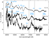 |
Fig. 3. Optical spectral sequence of SN 2016jae. All spectra have been corrected by redshift and extinction. The grey columns show the location of the strongest telluric band, which has been removed when possible. The locations of the most prominent spectral features are also indicated. |
Motivated by the two preceding discoveries of nebular Hα lines in 100IAS, we inspected the spectra of SN 2016jae and noticed the presence of a significant Hα emission line. It is weak and barely visible at phase 84.0d but seen clearly at phase 141.8d (see also the two-dimensional image of the spectrum in Fig. 4 and the Hα line profile comparison in Fig. A.5, which support our belief that the Hα line is intrinsic to the SN spectrum and not a contamination from nearby galaxy background). This same line is also present in the nebular spectra of SNe 2018cqj and 2018fhw at similar phases, as can be seen in the left panel of Fig. 5. The Hα line of SN 2016jae appears on top of a broader feature, probably due to a blend of iron-group elements (see e.g., Mazzali et al. 1997). We decomposed the line profiles into three Gaussian profiles, one for the narrow Hα and two components to match the broad iron-peak element feature (see Elias-Rosa et al. 2016 for more details on the procedure). The right panels of Fig. 5 show the result of the multi-component fit. The profiles are well reproduced with a narrow component centred at ∼6568 Å rest frame, with full width at half maximum (FWHM) of ∼16 Å (∼650 km s−1; after correction for instrumental resolution13) at phase 84.0d, and at ∼6567 Å, with FWHM of ∼22 Å (∼1000 km s−1) at phase 141.8d. The integrated luminosity of Hα was estimated to be L(84.0d) = (3.0 ± 0.8)×1038 erg s−1 and L(141.8d) = (1.6 ± 0.2)×1038 erg s−1. The best-fit luminosity of the Hα line decreases by a factor of ∼2 between the 84.0 and 141.8 day spectra; however, given the error of the flux measurement in the first epoch, we cannot exclude that the flux could remain constant. In the case of SN 2016jae, as well as in SNe 2018cqj and 2018fhw, the Hβ is not visible. Following the method introduced by Tucker et al. (2020), we estimated a 10σ upper limit on the Hβ flux of the order of ∼10−17 erg s−1 cm−2. A similar result was also obtained for SNe 2018cqj and 2018fhw.
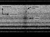 |
Fig. 4. Hα emission line in the two-dimensional spectrum of SN 2016jae taken with GTC/OSIRIS on 2017 May 18 (phase 141.8 d from the assumed B maximum date). The wavelength is up, and the spatial direction is to the right. |
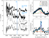 |
Fig. 5. Hα emission lines in the late-time optical spectra of SN 2016jae. Left: comparison of SN 2016jae late-time optical spectra, along with those of the SNe 2018cqj and 2018fhw at similar epochs. All spectra were redshift and reddening corrected (values adopted from the literature; see also Table B.1). Ages are relative to B maximum light. The locations of the Hα emission line are also indicated. Right: decomposition of the Hα emission line of SN 2016jae at phases 84.0 (top) and 141.8 d (bottom). Three Gaussian profiles have been used, for the narrow Hα and the two broad components of iron-group elements. |
4. Discussion and summary of the nature of SN 2016jae and its progenitor scenario
In the previous sections we have analysed the observed properties of SN 2016jae. This SN, classified as a Type Ia, shows a B-band peak of −17.93 ± 0.11 mag, an intermediate value between that of SN 2011fe (a normal SN; MB, max = −19.1, Ashall et al. 2016) and SN 1991bg (a sub-luminous SN prototype; > –17.7 mag, Taubenberger et al. 2017), followed by a fast decrease with Δm15 of 1.88 ± 0.10 mag. Despite its early classification as a normal SN Ia, the SN observables of SN 2016jae point to a similarity with fast-declining and sub-luminous transitional events. The noticeable feature is a narrow Hα line that appears in the nebular spectra. This emission line is associated with the SN, and the velocities are 650 and 1000 km s−1 at phase 84d and 142d, respectively. The derived FWHM is similar to those obtained for SNe 2018cqj and 2018fhw (∼1200 km s−1 at 193d and 139d, respectively), the two other low-luminosity SNe Ia with detection of Hα emission line in late-time spectra.
Understanding the origin of this H emission can give crucial constraints for the progenitor scenario. We first consider two scenarios: (i) pre-existing CSM material shocked by the SN ejecta and (ii) material stripped by the SN ejecta from an H-rich companion star in a single-degenerate progenitor system.
Nearby CSM can originate from the system before explosion due to the outcome of a common envelope phase. In this case, the expected expansion velocity of Hα is of the order of a few hundred km s−1, comparable to that presumed for interacting SNe (e.g., Silverman et al. 2013; Smith 2014). However, the estimated velocities for SNe 2016jae, 2018cqj, and 2018fhw are much higher. Additionally, Hα should also appear at early phases and accompanied by other Balmer emissions, such as Hβ (we noted the non-detection of Hβ in SN 2016jae in Sect. 3.2). In short, it is unlikely that the gas shell was produced by a common envelope phase. Also, the parent stellar population of these three transitional SNe Ia with Hα emission was most likely old. In fact, both SNe 2018cqj and 2016jae appeared in the outskirts of their putative host galaxies, suggesting that they are halo objects, whereas the host of SN 2018fhw was a dwarf elliptical. This is consistent with the progenitor environment of the majority of the 91bg-like and transitional SNe (see e.g., Panther et al. 2019) rather than with that of SNe Ia-CSM, which are found in star-forming galaxies (see e.g., Hamuy et al. 2003; Prieto et al. 2007; Dilday et al. 2012; Silverman et al. 2013).
An alternative is that SN 2016jae exploded in a single-degenerate system and that the H material was stripped from the non-degenerate H-rich companion star. It is expected that the stripped material has expansion velocities of ≤1000 km s−1 (see e.g., Mattila et al. 2005; Liu et al. 2012), which is consistent with the estimated velocity from the Hα line in SN 2016jae. In recent simulations, Dessart et al. (2020) found that the hydrogen stripped from a non-degenerate companion star can remain undetected at epochs of < 50d and begin to emerge at 100d, becoming clearly visible between 150d and 200d (at this time the metal-rich ejecta become increasingly fainter and more transparent). This is fully consistent with our observations of SN 2016jae. Additionally, these authors argue that we may see Hα and not Hβ because Hα sits in one of the most transparent regions of the optical range, while Hβ occurs in a region with strong metal line blanketing. It should be noted that stripping could also be asymmetrical and the cause of the possible redshift of ∼200 km s−1 in the Hα profile (at both the 84d and 142d phases for the adopted zhost = 0.021; Prieto et al. 2020; Botyánszki et al. 2018). In fact, Prieto et al. (2020) stressed that the apparent line shift may be related to the uncertainties in the location and redshift of the SN. It may be a concern for SN 2016jae because, as discussed in Sect. 2, it is not clear which galaxy hosts this SN. However, assuming zhost = 0.019, the Hα peak would be even more blue-shifted, by ∼800 km s−1.
As in SNe 2018cqj and 2018fhw, we can use the luminosity estimation from the nebular spectra and constrain the amount of hydrogen stripped from the non-degenerated companion star. Using the relation introduced by Tucker et al. (2020), which is based on the models of Botyánszki et al. (2018), we can derive a mass of the hydrogen-stripped material (Mst) of 0.002 M⊙ from the two nebular spectra of SN 2016jae. Similarly, following Dessart et al. (2020) and considering the estimated 56Ni mass for SN 2016jae in Sect. 3.1 (0.15 M⊙14), we obtain a comparable value for Mst of 0.003 M⊙. This estimated Mst is similar to that found for SNe 2018cqj and 2018fhw, and, as already noticed by Dessart et al. (2020), it is much lower than expected (> 0.1 M⊙) for standard models of single-degenerate scenarios for SNe Ia (see e.g., Marietta et al. 2000; Liu et al. 2012; Botyánszki et al. 2018). We attempted to understand the evolution with time of the Hα luminosity by considering the measurements for the three SNe with detected hydrogen. As we see in Fig. 6, the Hα luminosity decreases with the phase of the SN. Dessart et al. (2020) showed that the luminosity of Hα accounts for 10% of the radioactive decay energy absorbed by the stripped gas. This dependence implies a connection between the Hα luminosity and the characteristic time of the 56Co decay. That is, the luminosity of Hα decreases with time, and this is faster when Mst is low. This is related to the fact that γ rays are not efficiently trapped by the stripped material when Mst is low.
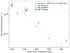 |
Fig. 6. Evolution of the luminosity of Hα of SNe 2016jae, 2018cqj, and 2018fhw. For comparison, we have also plotted an average value for the subset of models with Mst = 0.0018M⊙ of Dessart et al. (2020) (dotted line). For the SNe of the sample, we have assumed 15 days of rise time (average from the values found by Hsiao et al. 2015 and Vallely et al. 2019). |
To check our estimates of the stripped mass derived from the Hα luminosity, we measured the equivalent width of this emission line, which is a parameter that does not depend on the distance or extinction of the object. For this, we followed the steps described in Dessart et al. (2020) and applied their analytical fit for a DDC2515 model. We obtained a Mst of 0.014 and 0.066 M⊙ at 84d and 142d, respectively, which is consistent with the values derived above.
In conclusion, while the H emission observed in SN 2016jae may be from material stripped from a companion, this seems in conflict with the Mst predicted by hydrodynamic models for this type of scenario. However, some mechanism may be hiding the stripped hydrogen gas. For example, some of the H-rich material may not be visible because it is travelling at higher velocities (although models predict that the amount of this high-velocity material is low; see e.g., Pan et al. 2012; Liu et al. 2012). Otherwise, the outer layer of the companion star might have been stripped off by an optically dense wind well before the explosion (Hachisu et al. 1999, 2008).
A key characteristic of SN 2016jae is the Hα expansion velocity of ∼1000 km s−1. Such a velocity can be reached by optically thick winds and nova ejecta (Hachisu et al. 1999; Moriya et al. 2019).
Based on this suggestion, one could consider a binary system made of a WD and a secondary H-rich star that is transferring mass to the WD. When the mass transfer rate becomes larger than the maximum accretion rate for stable H-shell burning on the surface of the WD, the unprocessed material is expelled in the form of an optically thick wind (see e.g., Wang 2018). If the WD explodes during the wind phase, the resulting SN Ia could show the presence of hydrogen (Hachisu et al. 1999; Kato & Hachisu 2012). Alternatively, the high mass transfer rate may lead to a long series of relatively mild nova eruptions. These nova cycles cause the initial CO WD to grow in mass until it reaches masses of the order of 1.35–1.38 M⊙ and finally to explode as an SN (see e.g., Hillman et al. 2016 or Hachisu & Kato 2018). This is not the first time that a recurrent nova has been proposed as the progenitor of SNe Ia, although this scenario was more often called on to explain SNe interacting strongly with the CSM at early times (see e.g., Dilday et al. 2012; Wood-Vasey & Sokoloski 2006; Hachisu & Kato 2018).
There may be other possibilities that we have not discussed in detail here. For example, as recalled by Dessart et al. (2020), the enclosed (> 0.1 M⊙) H-rich material that moves at low velocity may originate from a tertiary star in a triple system or a swept-up giant planet rather than from a non-degenerate companion star (Soker 2019).
Altogether, the observables of SNe 2016jae, 2018cqj, and 2018fhw suggest that they could be transition objects between normal SNe Ia and low peak luminosity SNe Ia. The fact that these three SNe share, among their many similarities, the presence of H at similar dates is suggestive and raises the possibility of a common progenitor system. Certainly, the Zorro Diagram, which includes a large sample of well-observed luminous, normal, and sub-luminous SNe Ia (Mazzali et al. 2007), suggests that all the SNe considered in this analysis have a similar mass progenitor, consistent with the Chandrasekhar model. However, Dessart et al. (2020) show a better fit of the optical spectrum of SN 2018cqj at 207d after explosion (Prieto et al. 2020) with a mass that is lower than the Chandrasekhar mass. Indeed, there is growing evidence that the properties of low-luminosity SNe are better explained by a sub-Chandrasekhar mass explosion (Stritzinger et al. 2006; Scalzo et al. 2019). At the same time, from a theoretical point of view, the single-degenerate scenario for transitional SNe Ia has been ruled out based on the t0–M56Ni relation (Wygoda et al. 2019; Sharon & Kushnir 2020). However, the appearance of hydrogen at nebular phases appears to not be generally expected from the double-degenerate scenario or, in turn, with the sub-Chandrasekhar model for the three SNe of our sample. In short, at the present stage, we cannot link the ‘coincidence’ of these three SNe to a unique evolution scenario or explosion mechanism.
The particular case of the SN Ia 2015cp (Graham et al. 2019), an SN 1991T-like over-luminous Ia with narrow Hα appearing at nearly 2 years post-explosion, should also be noted.
An uncertainty of the velocity of 250 km s−1 was added in quadrature to the distance error (see Burns et al. 2018).
The NASA/IPAC Extragalactic Database (NED) is funded by the National Aeronautics and Space Administration (NASA) and operated by the California Institute of Technology.
Collection of a Complete, Nearby, and effectively unbiased sample of SNe Ia at host-galaxy redshifts zhost < 0.02.
SNOoPy is a package for SN photometry using PSF fitting and/or template subtraction developed by E. Cappellaro. A package description can be found at http://sngroup.oapd.inaf.it/ecsnoopy.html.
Our estimation of 56Ni mass for SN 2018fhw is consistent with the value derived by Vallely et al. (2019), 0.2 M⊙
The spectrum was taken from WiseREP (Yaron & Gal-Yam 2012); https://wiserep.weizmann.ac.il.
FAINT SNe Ia (one of the three families grouped by Benetti et al. 2005 according to observed diversities) are characterized by having low expansion velocities and a rapid evolution of the Si II velocity. In the classification scheme of Branch et al. (2006), the CL (or cool) SNe Ia are those with moderate values of pseudo-equivalent width of the Si IIλ6355 line but large values of pseudo-equivalent width of the Si IIλ5972 line.
For the resolved narrow line components, we first corrected the measured FWHM for the spectral resolution ( ) and then computed the velocity (v = width × c).
The value of the 56Ni mass allows us to discriminate between the models used by Dessart et al. (2020) for the analytical fit to the correlation between the luminosity of Hα and Mst. Here we have followed the delayed-detonation model DDC25 with a 56Ni mass of 0.12 M⊙.
Delayed-detonation model with a 56Ni mass of 0.12 M⊙ from Blondin et al. (2013).
Acknowledgments
N.E.R. thanks D. Kushnir, M. Hernanz and J. Isern for useful discussions and to the telescope’s staff for their excellent support in the execution of the observations. N.E.R. and E.C. acknowledge support from MIUR, PRIN 2017 (grant 20179ZF5KS). Support for J.L.P. is provided in part by ANID through the Fondecyt regular grant 1191038 and through the Millennium Science Initiative grant ICN12_009, awarded to The Millennium Institute of Astrophysics, MAS. Based on observations made with the GTC telescope, in the Spanish Observatorio del Roque de los Muchachos of the Instituto de Astrofísica de Canarias, in the island of La Palma. This paper includes data gathered with the 6.5 m Magellan Telescopes located at Las Campanas Observatory, Chile. We acknowledge ESA Gaia, DPAC and the Photometric Science Alerts Team (http://gsaweb.ast.cam.ac.uk/alerts). This work is based (in part) on observations collected at the European Organisation for Astronomical Research in the Southern Hemisphere, Chile as part of PESSTO, (the Public ESO Spectroscopic Survey for Transient Objects Survey) ESO program 188.D-3003, 191.D-0935, 197.D-1075. This research has made use of the NASA/IPAC Extragalactic Database, which is funded by the National Aeronautics and Space Administration and operated by the California Institute of Technology.
References
- Ashall, C., Mazzali, P., Sasdelli, M., & Prentice, S. J. 2016, MNRAS, 460, 3529 [NASA ADS] [CrossRef] [Google Scholar]
- Benetti, S., Cappellaro, E., Mazzali, P. A., et al. 2005, ApJ, 623, 1011 [NASA ADS] [CrossRef] [Google Scholar]
- Benetti, S., Cappellaro, E., Turatto, M., et al. 2006, ApJ, 653, L129 [NASA ADS] [CrossRef] [MathSciNet] [Google Scholar]
- Blondin, S., & Tonry, J. L. 2007, ApJ, 666, 1024 [NASA ADS] [CrossRef] [Google Scholar]
- Blondin, S., Dessart, L., Hillier, D. J., & Khokhlov, A. M. 2013, MNRAS, 429, 2127 [NASA ADS] [CrossRef] [Google Scholar]
- Blondin, S., Dessart, L., & Hillier, D. J. 2015, MNRAS, 448, 2766 [NASA ADS] [CrossRef] [Google Scholar]
- Botyánszki, J., Kasen, D., & Plewa, T. 2018, ApJ, 852, L6 [NASA ADS] [CrossRef] [Google Scholar]
- Branch, D., Dang, L. C., Hall, N., et al. 2006, PASP, 118, 560 [NASA ADS] [CrossRef] [Google Scholar]
- Brown, T. M., Baliber, N., Bianco, F. B., et al. 2013, PASP, 125, 1031 [NASA ADS] [CrossRef] [Google Scholar]
- Burns, C. R., Stritzinger, M., Phillips, M. M., et al. 2011, AJ, 141, 19 [NASA ADS] [CrossRef] [Google Scholar]
- Burns, C. R., Parent, E., Phillips, M. M., et al. 2018, ApJ, 869, 56 [NASA ADS] [CrossRef] [Google Scholar]
- Calzetti, D., Kinney, A. L., & Storchi-Bergmann, T. 1994, ApJ, 429, 582 [NASA ADS] [CrossRef] [Google Scholar]
- Chambers, K. C., Magnier, E. A., Metcalfe, N., et al. 2016, ArXiv e-prints [arXiv:1612.05560] [Google Scholar]
- Chen, P., Dong, S., Kochanek, C. S., et al. 2020, ArXiv e-prints [arXiv:2011.02461] [Google Scholar]
- Dessart, L., Leonard, D. C., & Prieto, J. L. 2020, A&A, 638, A80 [NASA ADS] [CrossRef] [EDP Sciences] [Google Scholar]
- Dilday, B., Howell, D. A., Cenko, S. B., et al. 2012, Science, 337, 942 [NASA ADS] [CrossRef] [Google Scholar]
- Dong, S., Katz, B., Kollmeier, J. A., et al. 2018, MNRAS, 479, L70 [NASA ADS] [CrossRef] [Google Scholar]
- Elias-Rosa, N., Pastorello, A., Benetti, S., et al. 2016, MNRAS, 463, 3894 [NASA ADS] [CrossRef] [Google Scholar]
- Filippenko, A. V., Richmond, M. W., Branch, D., et al. 1992, AJ, 104, 1543 [NASA ADS] [CrossRef] [Google Scholar]
- Graham, M. L., Harris, C. E., Nugent, P. E., et al. 2019, ApJ, 871, 62 [NASA ADS] [CrossRef] [Google Scholar]
- Gress, O., Lipunov, V., Buckley, D., et al. 2016, ATel., 9902, 1 [NASA ADS] [Google Scholar]
- Hachisu, I., & Kato, M. 2018, ApJS, 237, 4 [NASA ADS] [CrossRef] [Google Scholar]
- Hachisu, I., Kato, M., & Nomoto, K. 1999, ApJ, 522, 487 [NASA ADS] [CrossRef] [Google Scholar]
- Hachisu, I., Kato, M., & Nomoto, K. 2008, ApJ, 679, 1390 [NASA ADS] [CrossRef] [Google Scholar]
- Hamuy, M., Phillips, M. M., Suntzeff, N. B., et al. 2003, Nature, 424, 651 [NASA ADS] [CrossRef] [Google Scholar]
- Hillman, Y., Prialnik, D., Kovetz, A., & Shara, M. M. 2016, ApJ, 819, 168 [NASA ADS] [CrossRef] [Google Scholar]
- Hodgkin, S. T., Wyrzykowski, L., Blagorodnova, N., & Koposov, S. 2013, Philos. Trans. R. Soc. London Ser. A, 371, 20120239 [Google Scholar]
- Hsiao, E. Y., Burns, C. R., Contreras, C., et al. 2015, A&A, 578, A9 [NASA ADS] [CrossRef] [EDP Sciences] [Google Scholar]
- Kasen, D. 2006, ApJ, 649, 939 [NASA ADS] [CrossRef] [Google Scholar]
- Kato, M., & Hachisu, I. 2012, Bull. Astron. Soc. India, 40, 393 [NASA ADS] [Google Scholar]
- Kinney, A. L., Calzetti, D., Bohlin, R. C., et al. 1996, ApJ, 467, 38 [NASA ADS] [CrossRef] [Google Scholar]
- Kirshner, R. P., Jeffery, D. J., Leibundgut, B., et al. 1993, ApJ, 415, 589 [NASA ADS] [CrossRef] [Google Scholar]
- Kollmeier, J. A., Chen, P., Dong, S., et al. 2019, MNRAS, 486, 3041 [NASA ADS] [CrossRef] [Google Scholar]
- Krisciunas, K., Contreras, C., Burns, C. R., et al. 2017, AJ, 154, 211 [NASA ADS] [CrossRef] [Google Scholar]
- Leibundgut, B., Kirshner, R. P., Phillips, M. M., et al. 1993, AJ, 105, 301 [NASA ADS] [CrossRef] [Google Scholar]
- Liu, Z. W., Pakmor, R., Röpke, F. K., et al. 2012, A&A, 548, A2 [NASA ADS] [CrossRef] [EDP Sciences] [Google Scholar]
- Magnier, E. A., Schlafly, E. F., Finkbeiner, D. P., et al. 2020, ApJS, 251, 6 [Google Scholar]
- Maguire, K., Sullivan, M., Pan, Y. C., et al. 2014, MNRAS, 444, 3258 [NASA ADS] [CrossRef] [Google Scholar]
- Maoz, D., Mannucci, F., & Nelemans, G. 2014, ARA&A, 52, 107 [NASA ADS] [CrossRef] [Google Scholar]
- Marietta, E., Burrows, A., & Fryxell, B. 2000, ApJS, 128, 615 [NASA ADS] [CrossRef] [Google Scholar]
- Mattila, S., Lundqvist, P., Sollerman, J., et al. 2005, A&A, 443, 649 [NASA ADS] [CrossRef] [EDP Sciences] [Google Scholar]
- Mazzali, P. A., Chugai, N., Turatto, M., et al. 1997, MNRAS, 284, 151 [NASA ADS] [Google Scholar]
- Mazzali, P. A., Röpke, F. K., Benetti, S., & Hillebrandt, W. 2007, Science, 315, 825 [NASA ADS] [CrossRef] [PubMed] [Google Scholar]
- Moriya, T. J., Liu, D., Wang, B., & Liu, Z.-W. 2019, MNRAS, 488, 3949 [NASA ADS] [CrossRef] [Google Scholar]
- Nugent, P., Phillips, M., Baron, E., Branch, D., & Hauschildt, P. 1995, ApJ, 455, L147 [NASA ADS] [CrossRef] [Google Scholar]
- Pan, K.-C., Ricker, P. M., & Taam, R. E. 2012, ApJ, 750, 151 [NASA ADS] [CrossRef] [Google Scholar]
- Panther, F. H., Seitenzahl, I. R., Ruiter, A. J., et al. 2019, PASA, 36, e031 [NASA ADS] [CrossRef] [Google Scholar]
- Pereira, R., Thomas, R. C., Aldering, G., et al. 2013, A&A, 554, A27 [NASA ADS] [CrossRef] [EDP Sciences] [Google Scholar]
- Phillips, M. M. 2012, PASA, 29, 434 [NASA ADS] [CrossRef] [Google Scholar]
- Phillips, M. M., Lira, P., Suntzeff, N. B., et al. 1999, AJ, 118, 1766 [Google Scholar]
- Planck Collaboration XIII. 2016, A&A, 594, A13 [NASA ADS] [CrossRef] [EDP Sciences] [Google Scholar]
- Prieto, J. L., Garnavich, P. M., Phillips, M. M., et al. 2007, ArXiv e-prints [arXiv:0706.4088] [Google Scholar]
- Prieto, J. L., Chen, P., Dong, S., et al. 2020, ApJ, 889, 100 [NASA ADS] [CrossRef] [Google Scholar]
- Scalzo, R. A., Parent, E., Burns, C., et al. 2019, MNRAS, 483, 628 [Google Scholar]
- Schlafly, E. F., & Finkbeiner, D. P. 2011, ApJ, 737, 103 [NASA ADS] [CrossRef] [Google Scholar]
- Sharon, A., & Kushnir, D. 2020, Res. Notes. Am. Astron. Soc., 4, 158 [Google Scholar]
- Silverman, J. M., Foley, R. J., Filippenko, A. V., et al. 2012, MNRAS, 425, 1789 [NASA ADS] [CrossRef] [Google Scholar]
- Silverman, J. M., Nugent, P. E., Gal-Yam, A., et al. 2013, ApJS, 207, 3 [NASA ADS] [CrossRef] [Google Scholar]
- Smartt, S. J., Valenti, S., Fraser, M., et al. 2015, A&A, 579, A40 [NASA ADS] [CrossRef] [EDP Sciences] [Google Scholar]
- Smith, N. 2014, ARA&A, 52, 487 [Google Scholar]
- Smith, K. W., Cikota, A., Magee, M., et al. 2016a, ATel., 9908, 1 [NASA ADS] [Google Scholar]
- Smith, K., Cikota, A., Magee, M., Kankare, E., & Yaron, O. 2016b, Transient Name Server Classification Report 2016-1095, 1 [Google Scholar]
- Smith, K. W., Smartt, S. J., Young, D. R., et al. 2020, PASP, 132, 085002 [Google Scholar]
- Soker, N. 2019, Res. Notes Am. Astron. Soc., 3, 153 [CrossRef] [Google Scholar]
- Stritzinger, M., & Leibundgut, B. 2005, A&A, 431, 423 [NASA ADS] [CrossRef] [EDP Sciences] [Google Scholar]
- Stritzinger, M., Leibundgut, B., Walch, S., & Contardo, G. 2006, A&A, 450, 241 [NASA ADS] [CrossRef] [EDP Sciences] [Google Scholar]
- Stritzinger, M., Burns, C. R., Phillips, M. M., et al. 2010, AJ, 140, 2036 [NASA ADS] [CrossRef] [Google Scholar]
- Taubenberger, S. 2017, The Extremes of Thermonuclear Supernovae, ed. A. W. Alsabti, & P. Murdin (Cham: Springer), 317 [Google Scholar]
- Tonry, J., Denneau, L., Stalder, B., et al. 2016, Transient Name Server Discovery Report 2016-1077, 1 [Google Scholar]
- Tonry, J. L., Denneau, L., Heinze, A. N., et al. 2018, PASP, 130, 064505 [NASA ADS] [CrossRef] [Google Scholar]
- Tucker, M. A., Shappee, B. J., Vallely, P. J., et al. 2020, MNRAS, 493, 1044 [NASA ADS] [CrossRef] [Google Scholar]
- Turatto, M., Benetti, S., Cappellaro, E., et al. 1996, MNRAS, 283, 1 [NASA ADS] [CrossRef] [Google Scholar]
- Vallely, P. J., Fausnaugh, M., Jha, S. W., et al. 2019, MNRAS, 487, 2372 [NASA ADS] [CrossRef] [Google Scholar]
- Wang, B. 2018, Res. Astron. Astrophys., 18, 049 [NASA ADS] [CrossRef] [Google Scholar]
- Wood-Vasey, W. M., & Sokoloski, J. L. 2006, ApJ, 645, L53 [NASA ADS] [CrossRef] [Google Scholar]
- Wygoda, N., Elbaz, Y., & Katz, B. 2019, MNRAS, 484, 3941 [Google Scholar]
- Yaron, O., & Gal-Yam, A. 2012, PASP, 124, 668 [NASA ADS] [CrossRef] [Google Scholar]
Appendix A: Additional figures of SN 2016jae
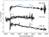 |
Fig. A.1. Spectra of SDSS-NW, SDSS-SW, and SDSS-SE taken with GTC/OSIRIS on 2019 December 3 and 2020 May 10. In particular, the spectrum of SDSS-SW is a combination of the spectra of both epochs. All spectra are in the rest frame and corrected for Galactic extinction. |
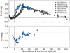 |
Fig. A.2. Intrinsic colour evolution of SN 2016jae, compared with those of SNe 1991bg, 2018cqj, 2018fhw, 1992A, and 2011fe. For both panels, the dot-dashed vertical line indicates the B-band maximum light. |
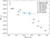 |
Fig. A.3. (Bmax-Vmax) colour vs. MBmax of a sample of sub-luminous SNe Ia (91bg-like) and transitional or 86G-like SNe from the Carnegie Supernova Project-I sample of Krisciunas et al. (2017). The magnitudes were derived using SNOoPy light curve fits, and the absolute magnitudes were calculated assuming H0 = 67.8 km s−1 Mpc. Magnitudes of SNe 1991bg, 2018cqj, 2018fhw, 1992A, 2011fe, and 2016jae are also plotted. |
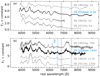 |
Fig. A.4. Early- (a) and late- (b) time comparison of SN 2016jae optical spectra, along with those of the sub-luminous SN 1991bg and the normal Ia SNe 1992A and 2011fe at similar epochs. All spectra have been corrected by redshift and extinction (adopted values and references are reported in Table B.1). Ages are relative to B maximum light. The grey columns show the location of the strongest telluric band, which has been removed when possible. |
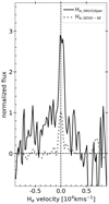 |
Fig. A.5. Hα line profile comparison of SN 2016jae at phase 141.8 d (from the assumed B maximum date) and the spectrum of SDSS-SE (the nearest galaxy with a similar redshift). The dashed lines mark the rest wavelength of Hα, and the normalized flux = 0. |
Appendix B: Properties of the supernovae used in this work
Properties of the SNe used in this work.
Appendix C: Tables of photometry and spectroscopy of SN 2016jae
New r (ABMAG) photometry of SN 2016jae.
Log of spectroscopy observations of SN 2016jae.
All Tables
All Figures
|
Fig. 1. Dark Energy Camera Legacy Survey (DECals) DR7 r deep image of the SN 2016jae field. The SN and the three nearby galaxies discussed in the text (SDSS-SW, SDSS-SE, and SDSS-NW) are indicated. We consider DL = 92.9 ± 4.3 Mpc to estimate the physical projected distance in the scale bar. We argue that SN 2016jae most likely exploded in the outer halo of SDSS-SE, as this is the nearest galaxy with a similar redshift. |
| In the text | |
|
Fig. 2. Optical broadband light curves of SN 2016jae. Left: BVri light curves of SN 2016jae. The light curves have been shifted for clarity by the amounts indicated in the legend. Right: absolute B light curve of SN 2016jae, shown along with those of SNe 1991bg, 2018cqj, 2018fhw, 1992A, and 2011fe. For both panels, the dot-dashed vertical line indicates the B-band maximum light. The uncertainties for most data points are smaller than the plotted symbols. |
| In the text | |
|
Fig. 3. Optical spectral sequence of SN 2016jae. All spectra have been corrected by redshift and extinction. The grey columns show the location of the strongest telluric band, which has been removed when possible. The locations of the most prominent spectral features are also indicated. |
| In the text | |
|
Fig. 4. Hα emission line in the two-dimensional spectrum of SN 2016jae taken with GTC/OSIRIS on 2017 May 18 (phase 141.8 d from the assumed B maximum date). The wavelength is up, and the spatial direction is to the right. |
| In the text | |
|
Fig. 5. Hα emission lines in the late-time optical spectra of SN 2016jae. Left: comparison of SN 2016jae late-time optical spectra, along with those of the SNe 2018cqj and 2018fhw at similar epochs. All spectra were redshift and reddening corrected (values adopted from the literature; see also Table B.1). Ages are relative to B maximum light. The locations of the Hα emission line are also indicated. Right: decomposition of the Hα emission line of SN 2016jae at phases 84.0 (top) and 141.8 d (bottom). Three Gaussian profiles have been used, for the narrow Hα and the two broad components of iron-group elements. |
| In the text | |
|
Fig. 6. Evolution of the luminosity of Hα of SNe 2016jae, 2018cqj, and 2018fhw. For comparison, we have also plotted an average value for the subset of models with Mst = 0.0018M⊙ of Dessart et al. (2020) (dotted line). For the SNe of the sample, we have assumed 15 days of rise time (average from the values found by Hsiao et al. 2015 and Vallely et al. 2019). |
| In the text | |
|
Fig. A.1. Spectra of SDSS-NW, SDSS-SW, and SDSS-SE taken with GTC/OSIRIS on 2019 December 3 and 2020 May 10. In particular, the spectrum of SDSS-SW is a combination of the spectra of both epochs. All spectra are in the rest frame and corrected for Galactic extinction. |
| In the text | |
|
Fig. A.2. Intrinsic colour evolution of SN 2016jae, compared with those of SNe 1991bg, 2018cqj, 2018fhw, 1992A, and 2011fe. For both panels, the dot-dashed vertical line indicates the B-band maximum light. |
| In the text | |
|
Fig. A.3. (Bmax-Vmax) colour vs. MBmax of a sample of sub-luminous SNe Ia (91bg-like) and transitional or 86G-like SNe from the Carnegie Supernova Project-I sample of Krisciunas et al. (2017). The magnitudes were derived using SNOoPy light curve fits, and the absolute magnitudes were calculated assuming H0 = 67.8 km s−1 Mpc. Magnitudes of SNe 1991bg, 2018cqj, 2018fhw, 1992A, 2011fe, and 2016jae are also plotted. |
| In the text | |
|
Fig. A.4. Early- (a) and late- (b) time comparison of SN 2016jae optical spectra, along with those of the sub-luminous SN 1991bg and the normal Ia SNe 1992A and 2011fe at similar epochs. All spectra have been corrected by redshift and extinction (adopted values and references are reported in Table B.1). Ages are relative to B maximum light. The grey columns show the location of the strongest telluric band, which has been removed when possible. |
| In the text | |
|
Fig. A.5. Hα line profile comparison of SN 2016jae at phase 141.8 d (from the assumed B maximum date) and the spectrum of SDSS-SE (the nearest galaxy with a similar redshift). The dashed lines mark the rest wavelength of Hα, and the normalized flux = 0. |
| In the text | |
Current usage metrics show cumulative count of Article Views (full-text article views including HTML views, PDF and ePub downloads, according to the available data) and Abstracts Views on Vision4Press platform.
Data correspond to usage on the plateform after 2015. The current usage metrics is available 48-96 hours after online publication and is updated daily on week days.
Initial download of the metrics may take a while.