| Issue |
A&A
Volume 650, June 2021
|
|
|---|---|---|
| Article Number | A158 | |
| Number of page(s) | 21 | |
| Section | Stellar structure and evolution | |
| DOI | https://doi.org/10.1051/0004-6361/202140707 | |
| Published online | 24 June 2021 | |
A confined dynamo: Magnetic activity of the K-dwarf component in the pre-cataclysmic binary system V471 Tauri
1
Konkoly Observatory, Research Centre for Astronomy and Earth Sciences, Konkoly Thege út 15-17, 1121 Budapest, Hungary
e-mail: This email address is being protected from spambots. You need JavaScript enabled to view it.
2
Institute of Physics/IGAM, University of Graz, Universitätsplatz 5, 8010 Graz, Austria
3
Baja Astronomical Observatory of University of Szeged, Szegedi út, Kt. 766, 6500 Baja, Hungary
4
Leibniz-Institute for Astrophysics (AIP), An der Sternwarte 16, 14482 Potsdam, Germany
Received:
2
March
2021
Accepted:
10
April
2021
Abstract
Context. Late-type stars in close binary systems can exhibit strong magnetic activity owing to rapid rotation supported by tidal locking. On the other hand, tidal coupling may suppress the differential rotation which is a key ingredient of the magnetic dynamo.
Aims. We studied the red dwarf component in the eclipsing binary system V471 Tau in order to unravel the relations between the different activity layers, from the stellar surface through the chromosphere up to the corona. Our aim is to study how the magnetic dynamo in the late-type component is affected by the close white dwarf companion.
Methods. We used space photometry, high-resolution spectroscopy, and X-ray observations from different space instruments to explore the main characteristics of magnetic activity. We applied a light curve synthesis program to extract the eclipsing binary model and to analyze the residual light variations. Photometric periods were obtained using a Fourier-based period search code. We searched for flares by applying an automated flare detection code. Spectral synthesis was used to derive or specify some of the astrophysical parameters. Doppler imaging was used to reconstruct surface temperature maps, which were cross-correlated to derive surface differential rotation. We applied different conversion techniques to make it possible to compare the X-ray emissions obtained from different space instruments.
Results. From the K2 photometry we found that 5–10 per cent of the apparent surface of the red dwarf is covered by cool starspots. From seasonal photometric period changes we estimated a weak differential rotation. From the flare activity we derived a cumulative flare frequency diagram which suggests that frequent flaring could have a significant role in heating the corona. Using high-resolution spectroscopy we reconstructed four Doppler images for different epochs which reveal an active longitude, that is, a permanent dominant spot facing the white dwarf. From short term changes in the consecutive Doppler images we derived a weak solar-type surface differential rotation with αDR = 0.0026 shear coefficient, similar to that provided by photometry. The long-term evolution of X-ray luminosity reveals a possible activity cycle length of ≈12.7 yr, traces of which were also discovered in the Hα spectra.
Conclusions. We conclude that the magnetic activity of the red dwarf component in V471 Tau is strongly influenced by the close white dwarf companion. We confirm the presence of a permanent dominant spot (active longitude) on the red dwarf facing the white dwarf. The weak differential rotation of the red dwarf is very likely the result of tidal confinement by the companion. We find that the periodic appearance of the inter-binary Hα emission from the vicinity of the inner Lagrangian point is correlated with the activity cycle.
Key words: stars: activity / binaries: eclipsing / starspots / stars: flare / stars: late-type / stars: individual: V471 Tau
Bolyai János Research Fellow.
© ESO 2021
1. Introduction
Magnetic fields have a strong effect on stellar structure and, overall, on the long-term evolution of stars, including our Sun. Studying the manifestations of stellar magnetic activity, from photospheric starspots through the bright chromospheric features to the active corona, helps us understand the nature of the underlying magnetic dynamo, and eventually the magnetic evolution of stars. In the last few years it has become feasible to study flares on a large number of stars with the Kepler, K2, and ongoing TESS missions (e.g., Balona 2015). This continuous high-precision space photometry combined with high-resolution spectroscopic observations can reveal the connection between the occurrence rate of flares and spot distributions.
It has been learned that late-type stars in close binary systems can exhibit even stronger magnetic activity owing to rapid rotation supported by tidal locking (e.g., Hill et al. 2014). Tidal coupling, however, may suppress the differential rotation (Scharlemann 1982) which is a key ingredient of the magnetic dynamo. The recent study by Kővári et al. (2017) showed that the tidal effect of a close companion star has indeed a suppressive effect on differential rotation.
In our paper we studied the red dwarf component in the eclipsing binary system V471 Tau in order to explore the relations between the different activity layers from the stellar surface through the chromosphere up to the corona. V471 Tau appeared first in the literature as a spectroscopic binary in the General Catalogue of Stellar Radial Velocities (GCRV, Wilson 1953). The system located in the Hyades star cluster consists of a DA white dwarf primary with a K2V companion, forming a post-common envelope binary (PCEB) star. The age of the Hyades cluster of t ≈ 680 Myr provides an upper limit for the age of V471 Tau (Gossage et al. 2018). The binary is thought to be a pre-cataclysmic variable as well, which means that there is no significant mass transfer in the system because the K star does not fill its Roche lobe. The orbital period of the eclipsing system of 0.52118 d (for updated orbital parameters, see Vaccaro et al. 2015) is modulated on the long term, which was explained by a light-time effect due to the gravitational influence of a third body, possibly a brown dwarf (Guinan & Ribas 2001). As an alternative explanation, the Applegate mechanism was offered by Hardy et al. (2015), where eclipse timing variations were interpreted as changes in the quadrupole moment within the K2V star. Recently, Lanza (2020) has proposed a mechanism based on a permanent non-axisymmetric gravitational quadrupole moment. It is no exaggeration to say that V471 Tau is an actual astrophysical laboratory for studying many aspects of stellar evolution. The white dwarf primary with a surface temperature of ≈35 000 K has strong emission in the ultraviolet (UV), extreme ultraviolet (EUV), and X-ray regimes. In such PCEB systems X-ray emission can originate from either the white dwarf or the corona of the K star. Moreover, the hot primary can also heat the exposed hemisphere of the secondary. V471 Tau is a well-known variable at the high-energy electromagnetic regime as well, being observed during the Einstein (Young et al. 1983), IUE (Guinan & Sion 1984), EXOSAT (Jensen et al. 1986), and ROSAT (Barstow et al. 1992; Wheatley 1998) missions, and more recently in the course of the Chandra (García-Alvarez et al. 2005) and XMM-Newton missions, to mention the most important ones. Accordingly, among other major findings, Jensen et al. (1986) discovered the pulsation of the white dwarf, while Barstow et al. (1992) confirmed a weak accretion from the K star to the white dwarf via stellar wind. Using UV data from the Goddard high-resolution Spectrograph (GHRS) on board the Hubble Space Telescope, Bond et al. (2001) reported coronal mass ejections (CMEs) from the active K dwarf and estimated an emission rate of 100–500 CMEs per day (i.e., about one hundred times higher compared to the Sun).
The surface magnetic activity of the secondary, the K2V star, is forced to rotate synchronously with the orbital period, and is known to exhibit rotational variability due to starspots (e.g., Evren et al. 1986) and flare activity (Young et al. 1983). The first Doppler images of the star were presented by Ramseyer et al. (1995), who obtained four separate temperature maps spanning a year. In another Doppler imaging study Hussain et al. (2006) found that despite the tidally inhibited differential rotation the K-dwarf component of the V471 Tau binary system showed a high level of magnetic activity. For our paper we performed a complex study of the magnetic activity of V471 Tau, including new Doppler images and flare statistics for the spotted red dwarf.
The paper is organized as follows. In Sect. 2 we summarize the available photometric and spectroscopic data to be analyzed. In Sect. 4, using Kepler K2 observations and by extracting orbital solutions, we analyze light variations due to spots and flares. In Sect. 3, by means of spectral synthesis, we derive the precise astrophysical parameters of the active K-dwarf component, which is used to perform a Doppler imaging study in Sect. 5 where we estimate the surface differential rotation of the spotted star. The chromospheric and coronal activity of the K star is analyzed in Sect. 6. Our results are discussed in Sect. 7, and summarized in Sect. 8.
2. Data
2.1. K2 photometry
The Kepler K2 mission provided long-term high-precision space photometry (Howell et al. 2014) of V471 Tau (EPIC 210619926). The star was observed as part of the fourth campaign of the mission between 8 February and 20 April 2015 (BJD 2457061.7910−2457132.6877), covering 136 subsequent orbital cycles. Both short- (1 min) and long-cadence (30 min) light curves of V471 Tau are available for the interval. Although the K2 data do not coincide with the spectroscopic observations used in this paper, the short-cadence space data are suitable for studying spot evolution and flare activity on a somewhat longer timescale. As an example, in Fig. 1 we plot a part of the short-cadence light curve (two cycles) where in-eclipse and out-of-eclipse flares are also seen.
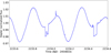 |
Fig. 1. Part of the Kepler K2 short-cadence data of V471 Tau with a particular flare event occurred when the white dwarf component was in eclipse. |
2.2. High-resolution spectroscopy
We use high-resolution (R = 81 000) spectroscopic observations of V471 Tau, publicly available in the data archive of the Echelle SpectroPolarimetric Device for the Observation of Stars (ESPaDOnS) at the Canada-France-Hawaii Telescope (CFHT). The spectra cover the 3700–10 500 Å optical range. The available data were retrieved in two seasons, the first in December 2005 and the second at the turn of 2014–2015. We selected 297 and 222 spectra from the two seasons, respectively, to achieve complete subsets (in the long run, two in both seasons for a total of four) with regard to optimal phase coverage for Doppler imaging (see Sect. 5). Low-quality spectra with a signal-to-noise ratio (S/N) < 40 were omitted from the selection. Before using the four data subsets for Doppler image reconstructions, we shifted the spectra to the rest wavelength, and continuum fitting was carried out. The CFHT spectra contain the Hα region which was used to study the chromospheric activity and discover possible mass motions in the binary (see Sect. 6.1). The observing log of the CFHT-ESPaDOnS spectra used in our study is given in Table A.1.
2.3. X-ray observations
The V471 Tau system has been detected with many X-ray instruments during the last decades. Here we attempt to infer the long-term variability of the K dwarf’s coronal emission. As none of the X-ray observations coincide with the epochs of the high-resolution spectroscopic data for Doppler imaging, we do not address its variability on shorter timescales, such as rotational modulation due to the distribution of active regions. We note that the binary components are not spatially resolved in the X-ray observations, but it is well established that only the softer wavelength range (> 50 Å) is affected by the emission from the white dwarf (Drake & Sarna 2003; García-Alvarez et al. 2005); therefore, its eclipse (at ϕ = 0 orbital phase) is only observed in EUV and soft X-ray (Cully et al. 1996; Wheatley 1998). What makes the investigation of the long-term coronal variability difficult is that V471 Tau was rarely observed by the same instrument more than once, the only exception being the ROSAT pointed survey (twice during the same year) and XMM-Newton (separated by 15 years). Moreover, the K dwarf is very active due to its high rotation rate, so its emission is variable also on short timescales, including frequent flares, which makes the definition of a quasi-quiescent emission level during a given epoch difficult.
For the analysis we select data from five X-ray instruments covering the years 1991–2019 (Table 1). We do not include data from earlier instruments (EXOSAT, Einstein) and the ROSAT All Sky Survey (RASS) because of their softer wavelength coverage (including mainly white dwarf emission) and/or their short duration. When selecting the space data we considered the epochs of our new Doppler reconstructions as well (see Sect. 5). In Sect. 6.2 we describe the detailed analysis steps for each instrument and observation, and which data were taken from previous analyses in the literature.
Adopted X-ray observations of V471 Tau with their durations and the quiescent periods within them.
3. Stellar properties
3.1. Adopted parameters
The Gaia DR2 parallax of π = 20.957 ± 0.044 mas (Gaia Collaboration 2018) yields a distance of d = 47.72 ± 0.10 pc for V471 Tau. Assuming  for the brightest V magnitude observed so far in 2004 (cf. İbanoǧlu et al. 2005), removing
  as the contribution of the white dwarf (Rucinski 1981), and taking into account a maximum of
  interstellar extinction (cf. Taylor 2006), this distance yields an absolute visual magnitude of
  . Taking the BC = −0.257 bolometric correction from (Flower 1996) gives a bolometric magnitude of
  . This gives L/L⊙ = 0.41 ± 0.01 when using a value of
  for the Sun. On the other hand, when adopting R/R⊙ = 0.91 ± 0.02 (Vaccaro et al. 2015, see their Table 11) and Teff = 4980 K (see Sect. 3.2), the Stefan-Boltzmann law would give a L/L⊙ ratio of 0.46 ± 0.04, which is a bit higher, but still in fair agreement with the value obtained from the bolometric magnitude.
We performed a spectral energy distribution (SED) synthesis using the virtual observatory (VO) tool VOSA (Bayo et al. 2008) to build the SED of V471 Tau from the available VO catalogs. We used VOSA to collect archival photometry from the Tycho, SLOAN/SDSS, Gaia DR2, 2MASS, AKARI/IRC, and WISE surveys. As input we confined the effective temperature to 4950 K < Teff < 5050 K, the surface gravity to 4.25 < log g < 4.75, and the metallicity to −0.2 < [Fe/H]< 0.2 (see Sect. 3.2). The resulting synthetic spectrum plotted in Fig. 2 corresponds to L/L⊙ of 0.40 ± 0.21, in agreement with both of the values given above.
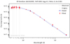 |
Fig. 2. Spectral energy distribution for V471 Tau generated by the VOSA SED analyzer tool (Bayo et al. 2008). The synthetic spectrum (blue line) is fitted to the available archival photometry (red dots) from the Tycho, SLOAN/SDSS, Gaia DR2, 2MASS, AKARI/IRC, and WISE surveys. |
The v sin i = 91 km s−1 projected rotational velocity of the K2 star was adopted from Hussain et al. (2006, see also their references). The inclination  of the binary orbit with respect to the line of sight was derived in O’Brien et al. (2001), which we adopt here for the K dwarf with the assumption that its rotational axis is perpendicular to the orbital plane.
Adopting the Porb = Prot period and the HJD0 = 2440610.06406 reference time (mid-primary minimum when the white dwarf is in eclipse) from Guinan & Ribas (2001) we use the following equation to calculate the phase values of the spectroscopic observations in Table A.1:
 (1)
(1)
3.2. Spectral synthesis
We carried out a detailed spectroscopic study based on spectral synthesis using the code SME (Piskunov & Valenti 2017). During the synthesis the MARCS models were used (Gustafsson et al. 2008) and the atomic parameters were taken from VALD (Kupka et al. 1999). The macroturbulence was computed using the following equation from Valenti & Fischer (2005):
![Mathematical equation: $$ \begin{aligned} { v}_{\mathrm{mac} }\, [\mathrm km\,s ^{-1}] =3.98-\frac{T_{\mathrm{eff} }\,\ [\mathrm{K}]-5770}{650}\cdot \end{aligned} $$](/articles/aa/full_html/2021/06/aa40707-21/aa40707-21-eq9.gif) (2)
(2)
First, we selected 15 good quality spectra observed in eclipses when only the K2 star was seen, and performed the synthesis independently for the 15 spectra to get Teff, log g, and [Fe/H]. We used the initial values as input for subsequent iterations. We gradually confined the microturbulence and the projected rotational velocity at  and v sin i = 91(±1) km s−1, respectively, in agreement also with literary values (see, e.g., Hussain et al. 2006; Adibekyan et al. 2012, and their references). Finally, the surface gravity was kept fixed at log g = 4.5, in agreement with earlier well-established values (see Vaccaro et al. 2015, and their references). In the end, the procedure resulted in Teff = 4980 K and [Fe/H] = 0.12. For details of the iterative fitting method see Kriskovics et al. (2019). The final astrophysical parameters with their errors are listed in Table 2.
Fundamental astrophysical data of the K2 dwarf component of V471 Tau.
In the second test we ran the synthesis for all the available CFHT spectra to see if the surface temperature varies along the orbital phase. Therefore, all of the previously derived parameters were kept fixed except for the surface temperature. The results are plotted in Fig. 3, demonstrating that the surface of the red dwarf is indeed the least affected around ϕ = 0.0 when the hot component is obscured. The temperature rise of ≈100 K at ϕ = 0.5 compared to the eclipse either in 2005 (blue dots in the figure) or 2014–2015 (red dots) may be due to the irradiation of the hot component, but surface activity can also play a role (see Sect. 7.2 for a discussion). Indeed, it is very likely that the stellar dynamo in the synchronously rotating red dwarf is affected by the close companion and therefore manifestations of magnetic activity may be coupled to the orbital phase (cf. Schrijver & Zwaan 1991).
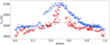 |
Fig. 3. Variation in the surface temperature of the K2 star along the orbital phase. The dots show the temperature values derived individually for each spectra (blue for the 2005 season, red for the 2014–2015 spectra) by spectral synthesis. Open circles around zero phase correspond to those unaffected spectra that were observed when the white dwarf was eclipsed. The temperature rise of ≈100 K at ϕ ≈ 0.5 in both seasons may indicate the irradiation effect of the hot component (see Sect. 3.2 for details). |
4. Photometric analysis
4.1. Extracting the eclipsing binary light curve
The entire K2 short-cadence data of V471 Tau covering 136 orbital cycles (≈71 d) are plotted in the upper panel of Fig. 4. The overall brightness variability is the result of a combination of several factors. The eclipses, the ellipsoidal variations and other possible binarity-related effects (reflection, irradiation) should also be considered. All of these effects are compounded by the changes resulting from the magnetic activity of the red dwarf star (i.e., surface spottedness and flares; see also Fig. 1).
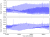 |
Fig. 4. K2 light curve of V471 Tau (top) and residual light variations (bottom) due to spots and flares after extracting the eclipsing binary model (see Sect. 4.1 for details). |
Before analyzing the photometric signs of the magnetic activity of V471 Tau, we removed the light curve variations caused by the close binary nature as follows. First we formed a phase-folded light curve with the use of the K2 short-cadence light curve. The data were grouped into 2000 orbital phase bins of equal duration. Then the average of each phase cell was calculated and rendered to the mid-phase point of the given cell. This way the fastest part of the non-orbital phase-locked light variations were removed, but a significant amount of the intrinsic variability over longer timescales was kept in the light curve. In order to remove these slower variations we synthesized a pure binary light curve with the use of the software package Lightcurvefactory (Borkovits et al. 2020). The input parameters were taken from Vaccaro et al. (2015). In addition to the eclipses, the binary model included ellipsoidal variations and the effect of Doppler-boosting. We did not consider, however, the reflection–irradiation effect, which was found to be negligible for the photometric contribution. Using the parameters from Vaccaro et al. (2015, see their Table 8, Col. 4) after a natural readjustment of the mid-time of a given eclipse (T0) parameter to the value appropriate for the K2 data, and comparing the synthesized light curve against the folded, binned, averaged K2 light curve, the residual curve showed significant “shoulders” around the partial phases of the eclipses, revealing that the durations of both the total eclipses and the totality should be slightly readjusted. We did this it manually with slight modifications of the radius of the K-dwarf component. This way we were able to remove the shoulders from the residual file. Finally, with a repeated use of Lightcurvefactory, this slightly refined synthetic light curve was removed from the original, ≈71 d long K2 measurements. The resulting residual light curve is plotted in Fig. 4.
4.2. Analyzing spot variability
As can be seen in Fig. 4, the light curve is solidly modulated by a continuously changing spot distribution. The relative intensity of the spot amplitude varies between 0.03 and 0.06. From this we estimate that 5–10 per cent of the apparent stellar surface is covered by spots (see Eq. (3) in Notsu et al. 2019). Assuming surface differential rotation, the change in the rotational frequency signals can be interpreted as a change in the latitude of the dominant surface spots. To recover the presence of differential rotation from the 136-cycle (≈71-day) photometric time series we applied the following technique. First, the entire residual light curve (bottom panel of Fig. 4) was divided into eight consecutive sections of ≈9 days (17 rotational cycles), which was a compromise to avoid averaging frequency signals over a longer timescale, but that still resulted in stable and/or reliable frequencies for the given part. To derive the most characteristic rotational period for each part we apply the Fourier-based period search code MuFrAn (Csubry & Kolláth 2004). The resulting short-term rotational periods listed in Table 3 indicate that the change in the period remains within a narrow interval of ΔP ≈ 0.001 day. Dividing this by the average rotation period from Table 2, we can estimate the dimensionless surface shear coefficient as  , where ΔPphot is the full range of the seasonal photometric period associated with surface spots, while
  is the average period over the long term. From the values listed in Table 3 we obtain |αDR|≳0.002 (i.e., a weak shear, almost solid body rotation). We note that this method alone does not allow us to determine the sign of the surface shear parameter (i.e., whether the differential rotation is solar type or antisolar).
Seasonal photometric periods from the K2 data.
4.3. Finding flares
After extracting the eclipsing binary model from the K2 light curve we searched for flares in the residual time series (bottom panel of Fig. 4.1) by applying the automated flare detection code FLAre deTection With Ransac Method (FLATW’RM; Vida & Roettenbacher 2018). The code allows the user to adjust the detection level and the number of successive points associated with a given flare. This is especially important when detecting the smallest events just above the noise level, which are always difficult to find. However, close to the noise limit the number of false positives starts to increase, which, on the other hand, can be compensated by increasing the number of associated points. After a visual inspection, however, we declared 15 false positives among the detected events. On the other hand, a similar number of possible flares just above the noise level could have been missed. For these reasons we ran a second analysis using a flare-searching neural network (Vida et al. 2021), and corrected its output manually for possible false positive or negative detections. This analysis yielded a final number of 198 confirmed flare events in the 71-day K2 time series.
Taking Teff and R from Table 2 the blackbody approximation yields Lq = 4.64 × 1032 erg s−1 quiescent luminosity for the K dwarf through the Kepler filter. To determine the individual flare energies, first the background variation (due to spots) is removed by fitting a low-order polynomial to the one-hour interval of the given flare (omitting the flaring points). The order of the polynomial is determined by the Bayesian information criterion. After subtracting this polynomial, the net flare light curve is integrated over the duration of the flare, yielding the εf relative flare energy (or equivalent duration) of the event. Multiplying εf with Lq gives the total energy Ef released by the flare. Finally, Ef values are used to make up the cumulative flare frequency diagram in Fig. 5.
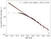 |
Fig. 5. Cumulative flare-frequency diagram for V471 Tau. The slope of the linear fit (orange line) corresponds to α = 1.8 power-law index. |
In principle, the cumulative number of flares versus flare energy can be described by a power law (Gershberg 1972). Accordingly, the logarithm of the ν(E) cumulative number of flares with energy values larger than or equal to E can be written as
 (3)
(3)
where c1 is the intercept and c2 is the slope of a linear function. Rewriting the slope c2 = 1 − α, we can introduce α, which is the power-law index of the flare energy distribution (Hawley et al. 2014). The low-energy turnover of the diagram below log E ≈ 32.6 [erg] is most probably the result of the detection threshold. Fitting the distribution above this turnover (red line in Fig. 5) yields a power-law index of α = 1.80 ± 0.01. For a further discussion of the flare statistics, see Sect. 7.3.
5. Doppler imaging
5.1. State-of-the art imaging code iMap
To reconstruct the surface temperature distribution map of V471 Tau we use the Doppler imaging code iMap (Carroll et al. 2012). This state-of-the-art code carries out multi-line inversion on a list of photospheric lines between 5000–6750 Å. We selected 24 non-blended absorption lines with suitable line-depth, temperature sensitivity and well-defined continuum. The stellar surface is modeled on a 5 ° ×5° resolution grid. Each local line profile is computed with a full radiative solver (Carroll et al. 2008). The local line profiles are disk integrated, and the individually modeled, disk-integrated lines are averaged. Atomic line data are from the Vienna Atomic Line Database (VALD; Kupka et al. 1999). Model atmospheres are from Castelli & Kurucz (2004) and were interpolated for the necessary temperature, gravity, or metallicity values. When solving the radiative transfer, local thermodynamical equilibrium (LTE) is assumed because spherical model atmospheres would have required too much computational capacity. Nevertheless, imperfections due to the LTE approximation in the fitted line shapes are well compensated by the multi-line approach. Additional input parameters are micro- and macroturbulence, and the projected equatorial velocity (see Sect. 3).
For the surface reconstructions iMap uses an iterative regularization based on a Landweber algorithm (Carroll et al. 2012). The iterative regularization has been proven to always converge on the same image solution (for the tests, see Appendix A in Carroll et al. 2012). Therefore, no additional constraints are imposed for the image reconstruction.
5.2. Surface temperature maps
In order to achieve sufficient phase coverage for the ≈0.52-day rotational period, we decided to form two subsets for each observing season. The first two sets, S1 and S2, are for the 2005 season; they consist of 149 and 172 spectra, respectively, both covering roughly four rotations (≈2 days). The S3 and S4 subsets are for the 2014–2015 season, and consist of 131 and 97 spectra; however, due to unfavorable data distribution in this season the S3 subset covers ≈20 consecutive rotations (≈10 days), while S4 covers 10 rotations (5 days); see Table A.1. All four subsets are used to reconstruct one Doppler image. The mean HJDs for the four subsets are 2453719.705, 2453722.211, 2457016.565, and 2457031.375, respectively. The four Doppler images (referred to hereafter as S1, S2, S3 and S4) presented below, can be regarded as snapshots of the stellar surface at these times.
5.2.1. Doppler images from the 2005 CFHT spectra
In Fig. 6 the two subsequent Doppler maps for the 2005 season (S1, S2) are plotted in orthographic projection in the quadrant phases of the rotation. The corresponding line profile fits are plotted in Figs. A.1 and A.2. Each temperature map shows mostly cool spots at similar locations, accounting for the reliability of the image reconstruction. Most of the cool surface features appear on the combined Doppler map derived from all of the spectra (S1+S2); see Fig. 7.
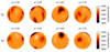 |
Fig. 6. Two Doppler images of V471 Tau from the 2005 data (S1 and S2). The surface temperature reconstructions are plotted in four rotational phases. |
 |
Fig. 7. Combined Doppler image of V471 Tau derived from all the available spectra from 2005 (S1+S2). The surface temperature map is plotted in four rotational phases. |
The strongest feature (a cool high-latitude spot on the hemisphere of the visible pole of ΔT < −1000 K temperature contrast relative to Teff) is shown on the S1 and S2 maps at around 0.45 phase, centered at β ≈ 50°. In addition, this large spot becomes more compact from S1 to S2. A mid-latitude spot is seen on the opposite (lower) hemisphere at ≈0.3 phase. Its location, however, shifts a bit from S1 to S2 toward the invisible pole or, alternatively, its extension decreases. A weak cool spot is seen on S1 at ≈0.13 phase, elongated from 30° latitude down to the equator, and even below to −30°. Such an elongated shape, however, may be the result of mirroring due to the high inclination. Its antitype on S2 is less contrasted, but more circular in shape and is confined to the upper hemisphere (i.e., it is less mirrored). Another less contrasted cool spot is seen on S2 centered at 0.83 phase and 20° latitude, which again has a weaker but more extended precursor on S1.
Some weak bright features are also seen, but the contrast hardly reaches ΔT ≈ +200 K, and their locations and shapes are more unpredictable when comparing the S1 image against S2. Their presence is even less salient on the average (S1+S2) image except the one at 0.3 phase. This feature, however, raises reliability issues. We know that spurious bright features can appear as an artifact of Doppler imaging coming from insufficient phase coverage (e.g., Lindborg et al. 2014). The phase coverages for both S1 and S2 were fairly good, the only remarkable phase gaps were between 0.288–0.500 and 0.171–0.318 in S1 and S2 datasets, respectively. This may explain the bright spot at 0.3 phase on the S2 reconstruction and account for some minor inconsistencies between S1 and S2 around these phase gaps. In conclusion, we think that those bright spots are mostly artifacts.
5.2.2. Doppler images from the 2014–2015 CFHT spectra
Doppler images for the 2014–2015 observing season (S3 and S4) are presented in Fig. 8; for the corresponding line profile fits see Figs. A.3 and A.4. Again, the most dominant cool features in two subsequent maps appear at similar locations. However, neither the weaker cool features nor the bright features are particularly consistent. For example, the bright features are more apparent in the S3 reconstruction than in S4. This is not surprising when keeping in mind that due to the unfavorable data distribution the selected spectra cover ≈20 days for S3 and 10 days for S4. Moreover, the time gap between the mean HJDs of S3 and S4 is ≈15 days; therefore incoherences between the two images are more visible. The combined Doppler map derived from all of the spectra (S3+S4) in Fig. 9 indicates that the most coherent and most striking feature is the high latitude (β ≈ 55°) cool spot at around ≈0.4 phase, recalling the S1 and S2 reconstructions. This cool spot may be coupled to the orbital phase, as suggested in Schrijver & Zwaan (1991). We conclude that the weak and inconsistent features in the S3 and S4 reconstruction, being cool or bright, can either be the result of imperfections of the reconstruction or come from the unfavorable conditions of the data distribution.
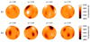 |
Fig. 8. Two Doppler images of V471 Tau for the second observing run at the turn 2014–2015 (S3 and S4). The surface temperature reconstructions are plotted in four rotational phases. |
 |
Fig. 9. Combined Doppler image of V471 Tau derived from all the spectra in the second observing run at the turn 2014–2015 (S3+S4). The surface temperature map is plotted in four rotational phases. |
5.3. Differential rotation
Surface differential rotation can be measured by longitudinally cross-correlating consecutive Doppler images (Donati & Collier Cameron 1997; Kővári et al. 2004), and fitting the latitudinal correlation peaks in the resulting cross-correlation function (ccf) map by a quadratic rotational law
 (4)
(4)
where Ω(β) is the angular velocity at β latitude, Ωeq is the angular velocity of the equator, and ΔΩ = Ωeq − Ωpole gives the difference between the equatorial and polar angular velocities. With these values, the dimensionless surface shear parameter αDR is defined as αDR = ΔΩ/Ωeq, leading to the following form:
 (5)
(5)
In our case two ccf maps can be composed, one for the two consecutive maps in the first observing season (S1, S2) and another for the two maps in the second season (S3, S4). After the necessary normalization procedure the two ccf maps are combined to get an average ccf map (for the applied method ACCORD; see, e.g., Kővári et al. 2012, 2015). The correlation pattern in the ultimate average ccf map (Fig. 10) is fitted by a rotational law according to Eq. (5). The resulting fit indicates a very weak solar-type differential rotation, with Ωeq = 691.57 ± 0.13° day−1 and αDR = 0.0026 ± 0.0006 shear parameter (i.e., almost solid body rotation) in fair agreement with the rough estimation from the K2 photometry (see Sect. 4.2). From the fitted Ωeq and αDR values we get βcor ≈ 43° for the co-rotating latitude (i.e., where rotation is synchronized exactly to the orbit).
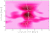 |
Fig. 10. Average cross-correlation function map derived from the subsequent Doppler images plotted in Figs. 6 and 8. Black represents strong correlation, while light pink indicates no correlation. The quadratic sine fit (solid line) applied to the ridge of the correlation pattern (dots with error bars) suggests a solar-type rotational law with a very weak shear of αDR = 0.0026 ± 0.0006. See Sect. 5.3 for details. |
6. Chromospheric and coronal activity
6.1. Variability of the Hα line profile
The Hα line profile variation is capable of unfolding chromospheric activity and presumably associated mass motions like CMEs. From the available time series of spectra we create time-slice plots for the two observing runs. The resulting dynamic spectra are shown in Figs. 11 and 12. The plot for the first observing run (S1+S2) indicates absorption around the 0.0 phase when the white dwarf is near or in eclipse. On the other hand, a strong emission develops around 0.35–0.6. Clearly, the peaks of the absorption and the emission profiles stay within the ±91 km s−1 projected equatorial velocity range of the K star, suggesting that the sources are related to some surface features. In particular, the emission around the secondary eclipse may indicate a relation with the dominant cool photospheric spot at around 0.45 phase (see Fig. 6). There may also be some extra emission on or over the receding side of the K star during the 0.2–0.3 phase; however, this part of the data has the lowest quality and even the phase coverage is not satisfactory, so we cannot make a definite statement about this feature.
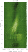 |
Fig. 11. Dynamic Hα spectrum from the 2005 data (S1+S2). The individual 1D Hα spectra along the orbital phase are plotted in the rest frame of the K star. Dark green corresponds to deep absorption, while light yellow indicates strong emission. The large amplitude (≈320 km s−1) sine curve is the radial velocity of the white dwarf; the smaller amplitude (≈150 km s−1) sinusoid is the radial velocity of the centre of mass of the binary system. The tick marks on the right indicate the phases of the observations. |
The Hα behavior from the 2014–2015 data (S3+S4) in Fig. 12 shows similarities to the dynamic Hα spectrum from the 2005 data, but quite different features are also present. Similar features are the absorption centered around the 0.0 phase and the emission during the 0.35–0.65 phase; this latter is less conspicuous but still around the phase of the most prominent cool spot (see Fig. 8). Being within the radial velocity range of the K dwarf, it is very likely that these features are localized on the surface of the red dwarf. However, in addition to the similarities there is a very different emitting phenomenon located between the centre of mass of the system and the white dwarf. This emission is stronger in the first half of the orbital phase, but still visible during the second half. This suggests the presence of a clump of emitting plasma corotating with the system in the vicinity of the inner Lagrangian (L1) point, as already reported by Young et al. (1991). We finally note that there may be some extra emission on the receding side of the K star around ϕ = 0.2, recalling Fig. 11, but the phase coverage is not satisfactory and the emission peaks are not as strong; therefore, again, we could only guess about its reliability, nature, and possible origin. For further discussion of the peculiar emission from beyond the L1 point see Sect. 7.4.
6.2. X-ray emission from the K dwarf
The ROSAT pointed observations from 1991 were analyzed by Wheatley (1998) who focused on the second longer exposure that we also use here. The full wavelength coverage of the PSPC detector is 0.1–2.5 keV (i.e., the softer part is dominated by the emission from the white dwarf). Wheatley (1998) presented the light curve of the observation in a soft (0.1–0.4 keV) and a hard (0.4–1.2 keV) band. The soft band clearly shows the partly covered eclipse, which is not seen in the hard band, confirming that the harder X-ray emission stems from the K dwarf only. Both bands show variability, but no large flares. The ROSAT data are, however, affected by many data gaps due to the spacecraft orbit. Therefore, we simply use the average flux from this observation as the quasi-quiescent state for this epoch. The 0.1–2.5 keV flux from the K dwarf only (determined by spectral modeling in Wheatley 1998) amounts to (4.0 ± 0.2) × 10−12 erg cm−2 s−1.
In 1996, V471 Tau was observed by ASCA. This observation is described and analyzed in detail by Still & Hussain (2003). Their light curve from the combined Solid-state Imaging Spectrometer (SIS) and Gas Imaging Spectrometer (GIS) data in the energy range 0.3–10 keV shows some variability that may be due to small flare events, but the number of potentially flaring data points is small compared to the full light curve. Still & Hussain (2003) used the whole observation for spectral modeling (due to the rather low count rate) and obtained an average flux of 2.4 × 10⁻¹² erg cm−2 s−1 that is valid for the 0.5–10 keV range, which we adopt here as well.
One year later, V471 Tau was observed with the ROSAT High Resolution Imager (HRI). This instrument has an energy range of 0.1–2.5 keV, but due to its negligible energy resolution the data cannot be binned in energy to remove the contribution from the white dwarf. Therefore, we extracted the light curve of the whole observation using the xselect task from the HEASoft1 package. This observation covered a part of one eclipse. Therefore, we used xselect to extract an image for the time interval of the eclipse only (thus containing only emission from the K dwarf) and determined the count rate with the ximage/sosta task, which also performs background subtraction and corrects for vignetting, deadtime, and point spread function (PSF). Although the full light curve did not show any large flares, the short duration of the usable time interval makes this data point more uncertain.
The Chandra observations from 2002 were analyzed in several studies (Drake & Sarna 2003; Ness et al. 2004; García-Alvarez et al. 2005). The HRC-S/LETG instrument provides high-resolution spectroscopy in the 0.07–7.29 keV range. The light curve shown by García-Alvarez et al. (2005) does not include any strong flares, so the average flux of the observation was adopted. This was taken from Ness et al. (2004) who extracted the flux in the smaller 5.15–38.19 Å wavelength band (quoted luminosity of 1.1234 × 1030 erg s−1) (i.e., with negligible contribution from the white dwarf).
The first XMM-Newton observation from 2004 was analyzed using the XMM-Newton Scientific Analysis System (SAS) Version 17.0.0. We only used data from the EPIC/PN detector, as the simultaneous EPIC/MOS and RGS data have lower signal-to-noise ratios. The SAS task epproc was used to create an event list from the raw odf file for the EPIC/PN detector. We extracted source and background regions in ds9 and use the SAS tasks evselect to create the light curves and epiclccorr to perform background subtraction and all necessary corrections (e.g., vignetting, deadtime, PSF). We used the energy band 0.3–10 keV to minimize potential contamination from the white dwarf at lower energies, and because we use this energy range for the common analysis of all instruments. This observation is affected by a large flare event previously analyzed by Pandey & Singh (2008) and by significant variability; therefore, we needed to use a restricted time range that most likely resembles a quasi-quiescent state. We extracted the last 18 783 s of the observation which seems to be free of any trends, although there is still strong scatter in the light curve.
In 2015, V471 Tau was observed by Swift. We inspected the light curves from the XRT instrument created by the online tool of the Swift Science Center2 (Evans et al. 2007, 2009). There are no strong flares in the data, so we simply adopted the averaged count rate from all observations in the 0.3–10 keV band.
The second XMM-Newton observation from 2019 was processed and analyzed in the same way as described before. This observation was also affected by a large flare and strong variability, which was required to extract the first 9381 s only, which seems to display a rather constant count rate without trends.
6.3. Evolution of the X-ray luminosity
To compare the X-ray emission from many different instruments it is necessary to either convert the fluxes taken from the literature to a common energy range or to obtain the appropriate count-to-flux conversion factors for the different instruments. We used the tool WebPIMMS3 to perform the necessary conversions. This requires input of the Galactic hydrogen absorption and a spectral model for the source.
To constrain the plasma parameters of the K dwarf in V471 Tau we performed spectral modeling of the two XMM-Newton data sets and Swift. For XMM-Newton, we extracted source and background spectra of the selected quasi-quiescent time ranges using evselect, and created the required redistribution matrix and auxiliary response files using rmfgen and arfgen. We used specgroup to group the files and selected a minimum of 20 counts per bin. We also used the option oversample set to 3, a usual value to avoid oversampling the intstrument resolution. We fitted the spectra using Xspec4 with a model including Galactic absorption and a sum of APEC (Smith et al. 2001) plasma models. As the Galactic absorption is not very well constrained by a fit to energy ranges > 0.3 keV, we fixed the H column density toward V471 Tau to its measured value of NH = 1.62 × 1018 cm−2 (Wood et al. 2005). This had a negligible effect on the results as this value is low because the star is nearby. For the fitting process we restricted the energy range further to 0.3–3.9 keV due to low signal at higher energies. At both epochs we find the best fits with two APEC plasma components with the same coronal abundances (Table 4). The results are broadly consistent with each other, and with other spectral analyses in the literature. We also tried to fit the Swift spectrum obtained from the online tool (Evans et al. 2009), but due to the small number of counts it was not possible to fit a 2-T plasma model. An acceptable fit was obtained for a 1-T model using the Cash statistics (Cash 1979), yielding a temperature comparable to the hotter component of the more reliable XMM-Newton fits and an emission measure similar to the total value obtained for XMM-Newton. All fits predict subsolar coronal abundances (Z ∼ 0.2 Z⊙), consistent with previous studies. Table 4 summarizes the plasma parameters obtained from the Xspec fits, together with the calculated average emission measure-weighted temperature Tav and total emission measure EMtot for the 2-T fits.
Spectral fits to the quiescent parts of the two XMM-Newton observations from 2004 and 2019 and the Swift data from 2015.
As we did not find significant differences of coronal plasma parameters from the analyzed observations, we adopted a common parameter set for all flux conversions. For simplicity, we used a 1-T APEC model in WebPIMMS with a mean temperature of 8.9 MK (log T = 6.95). We fixed the Galactic NH absorption to the value from Wood et al. (2005) and the coronal metal abundance to 0.2 Z⊙. Using a 2-T model with parameters similar to those obtained in the XMM-Newton fits did not change the results significantly. To estimate uncertainties for the conversion factors, we ran WebPIMMS with log T = 6.9 and log T = 7.0, corresponding to an uncertainty of the mean temperature by about 10%, which is slightly larger than we calculated from the XMM-Newton spectra (3–4%). This resulted in uncertainties on the conversion factors of ≲3%.
After converting the fluxes taken from the literature and the count rates of the specific instruments to a common energy range of 0.3–10 keV, we used the distance from Table 2 to convert the fluxes to luminosities. The results are shown in Fig. 13. The displayed uncertainties on the X-ray luminosities include the statistical uncertainties of the flux and count rate measurements, the flux conversion factors, and the distance. The X-ray luminosity of the K dwarf shows variations over the years; the maximum data point is 90% higher than the minimum. As there are only seven data sets spanning almost 30 years, some with exposure times for the quasi-quiescent time intervals as short as ∼20 min, a detailed investigation of a possible cycle was not feasible. Moreover, the data stem from a variety of different instruments, and cross-calibration issues are expected to be present (see the detailed discussion in Wargelin et al. 2017). To account for these instrument cross-calibration uncertainties, we added 10% to the luminosity uncertainties for the Chandra, XMM-Newton, and Swift data, and 20% for the older ROSAT and ASCA data (Snowden 2002; Tsujimoto et al. 2011).
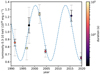 |
Fig. 13. Evolution of the X-ray luminosity of the K dwarf in V471 Tau from the observations summarized in Table 1. The duration of the selected quiescent ranges is color-coded. Solid error bars denote flux errors (see text); dotted bars are the estimated cross-calibration uncertainty. The blue dashed line indicates the best fit with a sinusoidal function with a period of ∼12.7 yr. |
Despite the limitations of the available data, we fit a sinusoidal function to the X-ray luminosities in Fig. 13. The blue dashed line in the plot corresponds to a period of about 12.7 yr, which can be interpreted as activity cycle. We note again, however, that the uneven spacing of the observations, the small number of data points, and the uncertainties of instrumental cross-calibration, do not allow a definitive conclusion about the existence of an X-ray cycle and its properties.
7. Discussions
7.1. Weak differential rotation and active longitude
From our Doppler reconstructions we measured a very weak solar-type surface differential rotation for the K star (Sect. 5.3). Such a weak shear, however, is not surprising as we essentially expect something similar for fast rotating late-type dwarf stars (see the empirical study by Kővári et al. 2017, and their references). In addition, synchronization due to tidal dissipation in close binaries may suppress the rotational shear (Scharlemann 1982). In Hussain et al. (2006) the authors reported almost rigid body rotation for V471 Tau with αDR of 0.0001 ± 0.0005 shear coefficient. In comparison, our result of αDR = 0.0026 ± 0.0006 is still weak, but an order of a magnitude stronger shear based on using much more data and our well-established cross-correlation technique ACCORD (for some applications and tests see, e.g., Kővári et al. 2004, 2012, 2014, 2015, and their references). This technique amplifies independent cross-correlation signals from different epochs to multiply the credibility and reliability of the result. We finally note that our larger shear coefficient is also supported by the short-term photometric period changes (see Sect. 4.2).
The Doppler reconstructions performed in our study indicate that the most dominant surface spot located at around 0.40–0.45 phase at β ≈ 50 − 55° latitude may be a permanent feature (see Figs. 6–8). In the Doppler imaging study by Ramseyer et al. (1995) the authors found that a dominant cool spot appeared at the longitude facing the white dwarf in all four of their Doppler maps (September 1992, October 1992, December 1992, and December 1993). Moreover, the Doppler image from November 2002 (Hussain et al. 2006) also indicated that the most prominent spot was directed toward the white dwarf.
Asymmetric tidal distortion may significantly alter internal dynamos of rapidly rotating convective stars in close binaries (Rottler et al. 2002), which can result in an active longitude around the sub-white dwarf point in the K-dwarf component. Such a non-axisymmetric nature of spot activity is not unusual in close binary systems (Oláh 2006). However, it has also been shown that the condition for the excitation of stable non-axisymmetric fields is weak differential rotation (Scharlemann 1982; Ruediger & Elstner 1994), which we firmly confirmed in the case of V471 Tau.
7.2. Effective temperature rise around ϕ = 0.5 phase
The ≈100 K variation of the surface temperature of the K dwarf along the orbital phase (see Fig. 3) may be interpreted as the irradiation effect of the white dwarf. We have no means to calculate what fraction of the radiative energy from the white dwarf is converted to thermal reprocessing in the photosphere of the K star. However, according to Young et al. (1988, their Table 2), the estimated ratio of the total luminous energy intercepted from the white dwarf to the bolometric output of the K star is ≈0.6% (i.e., below the detection limit of 3% assumed for such a heating mechanism to be efficient in the photosphere). A similar conclusion was drawn by O’Brien et al. (2001), who estimated that the luminosity of the K star would increase only by 1% due to the irradiation from the white dwarf, which would explain the only ≈12 K temperature rise of the sub-white dwarf hemisphere. In contrast, the effective temperature change of ≈100 K in Fig. 3 would assume ≈8% luminosity difference. At this point we speculate that the photospheric temperature rise around ϕ = 0.5 may instead be associated with increased magnetic activity at the sub-white dwarf hemisphere of the K star. It has been determined that faculae-dominated active stars tend to become brighter when their magnetic activity level increases (Radick et al. 1990). We believe that the hemispheric difference in magnetic activity observed in V471 Tau can have a significant effect on the overall hemispheric temperature difference as well (see, e.g., Gondoin 2008; Shapiro et al. 2016). This means that small-scale photospheric bright faculae, permanently present around the active longitude facing the white dwarf, may induce such a rise in the effective temperature.
7.3. Flare statistics
We find that the 198 flares detected in the 71-day K2 data of V471 Tau are distributed randomly over the rotational phase (i.e., no significant phase dependency was found in the flare occurrence). The derived flare energies in Sect. 4.3 range over four magnitudes. Recently, Kővári et al. (2020) have concluded that, in principle, differences between flare energies are due to size effect, regardless of energy range or spectral type (cf. Balona 2015). Accordingly, flare duration is supposed to increase with flare energy (cf. Houdebine 2003). In Fig. 14 we plot logΔt flare duration as a function of log Ef flare energy. The relationship on the log–log plot fitted by a linear function yields a 0.50 ± 0.02 slope. In comparison, Maehara et al. (2015) suggested a generalized function between flare duration and flare energy with a power-law index (slope) of ≈1/3.
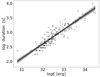 |
Fig. 14. Flare duration vs. flare energy from the K2 data of V471 Tau. The best fit indicates a power-law relationship with 0.5 ± 0.02 index. |
It has been suggested (see, e.g., Parker 1988; Hudson 1991; Saar & Bookbinder 1998) that the more numerous small flaring events have an important role in heating the plasma in the transition region and the corona. This is supported by the power-law index of α ≳ 2.0 derived from flare statistics of magnetically active M dwarf stars (e.g., Ilin et al. 2019, etc.). In comparison, α = 1.7 was obtained for 27 young K 5–7 stars in the Orion Nebula Cluster (Wolk et al. 2005). However, no such difference was found from the flare statistics for 548 M and 343 K-dwarf stars (α = 1.82 and 1.86, respectively) in Lin et al. (2019). Nevertheless, the α index of 1.8 obtained for V471 Tau (see Fig. 5) suggests that the dissipating energy of the flares should have a significant contribution in heating the upper atmosphere.
7.4. Inter-binary Hα emission during activity maximum
The cycle period of the sinusoid fitted to the X-ray luminosity variation in Fig. 13 is comparable to the 13 yr period identified in timing residuals by Vaccaro et al. (2015) and a possible ≈10 yr periodicity from an activity cycle mentioned by Kamiński et al. (2007). Moreover, Kamiński et al. (2007) stated that during observations with MOST in December 2005 the star was much less spotted than in the previous observations of Hussain et al. (2006) (from November 2002) and had very little photometric variability, which the authors interpreted as evidence that the K dwarf was close to an activity minimum. This is consistent with our fit to the X-ray data.
As Fig. 13 shows, about four months ahead of the epochs of the S1-S2 Doppler reconstructions (in 2004) the X-ray luminosity of V471 Tau was around its minimum. While about six months after the epochs of the S3-S4 Doppler images (in 2015) the X-ray luminosity was much higher, according to the data point from Swift. Oddly, such a large difference is not seen when comparing the overall spottedness in the S1-S2 images with that of S3-S4, which are quite similar, despite the ≈9-year time gap between them. However, the Hα line profile variability (see Figs. 11 and 12) showed very different behavior in the two observing runs. The extra Hα emission from the inter-binary space (see Fig. 12) might have something to do with the enhanced X-ray luminosity in 2015 (i.e., around activity maximum). This is supported by the result in Young et al. (1991, see their Fig. 3) who also found an external Hα emission component, originating from somewhere in the inter-binary space beyond the centre of mass of the system, expanding toward the white dwarf, definitely reminiscent of our result plotted in Fig. 12. Moreover, their observations were obtained in 3–4 November 1988 and 29–30 January 1989 (i.e., close to the suspected maximum of the activity cycle ended in 1994) (according to our Fig. 13). Further support can be found in Rottler et al. (2002) for the secular Hα variability in 1985, 1990, and 1992.
We expect that during the magnetic cycle, around activity maximum more and/or more extended magnetic loops develop high above the surface, reaching one stellar radius (Guinan et al. 1986), and in this way a greater amount of cool material enters the upper atmosphere in trapped clumps that are similar to solar prominences. Large prominence-like condensations of cool material were reported from Hα observations of AB Dor Collier Cameron & Robinson (1989), a single K0 dwarf that rotates as rapidly as V471 Tau. Normally, such a clump of cool material appears in absorption in Hα, exactly what we actually see on the far side of the K star around zero phase. However, it can get into emission when heated due to the UV radiation from the white dwarf. The physical process behind heating proposed first by Young et al. (1988) involves fluorescence-induced Hα emission (see also Bois et al. 1991). This scenario could explain the Hα line variability both around the activity minimum (Fig. 11) when there are no extended magnetic loops, and around maximum (Fig. 12) when extended loops with cool material trapped in them are present. Even so, we caution that our ground-based spectroscopic data and the space observations did not overlap exactly and the available space data is limited. Therefore, our conclusion about such a link between the peculiar Hα emission from the vicinity of the L1 point and the proximity of the activity cycle maximum may raise some criticism.
8. Conclusions
We studied the magnetic activity of the K-dwarf component in the close binary system V471 Tau in order to unravel how its magnetic dynamo is affected by the white dwarf. Our related concluding remarks are as follows:
-
We confirm that there is a permanent active longitude on the K star facing the white dwarf over decades, regardless of the actual phase of the magnetic cycle.
-
We confirm a weak solar-type surface differential rotation on the surface of the K star, supporting theoretical expectations.
-
We suggest that frequent flaring should have a significant contribution in heating the corona of the K star.
-
From the long-term evolution of X-ray luminosity we confirm a magnetic activity cycle of ≈12.7 yr, whose traces also appear in the chromospheric (Hα) activity pattern.
-
We find that the inter-binary Hα emission from the vicinity of the L1 point is correlated with the activity cycle: it intensifies during activity maximum and fades away during minimum.
That is, it definitely seems that the magnetic dynamo working in the red dwarf component is constrained by the close white dwarf companion.
Acknowledgments
This publication makes use of VOSA, developed under the Spanish Virtual Observatory project supported by the Spanish MINECO through grant AyA2017-84089. VOSA has been partially updated by using funding from the European Union’s Horizon 2020 Research and Innovation Programme, under Grant Agreement No. 776403 (EXOPLANETS-A). This research has made use of data, software and/or web tools obtained from the High Energy Astrophysics Science Archive Research Center (HEASARC), a service of the Astrophysics Science Division at NASA/GSFC and of the Smithsonian Astrophysical Observatory’s High Energy Astrophysics Division. This work made use of data supplied by the UK Swift Science Data Centre at the University of Leicester. Based on observations obtained with XMM-Newton, an ESA science mission with instruments and contributions directly funded by ESA Member States and NASA. This work was supported by the Hungarian National Research, Development and Innovation Office (NKFIH) grant K-131508 led by ZsK. Authors acknowledge the financial support of the Austrian-Hungarian Action Foundation (grants 101öu13 and 104öu2). LK acknowledges the financial support of the Hungarian National Research, Development and Innovation Office grant NKFIH PD-134784. TB is supported by the Hungarian National Research, Development and Innovation Office grant NKFIH KH-130372. KV acknowledges the financial support of the Hungarian National Research, Development and Innovation Office grants NKFIH KH-130526 and 2019-2.1.11-TT-2019-00056. ML and PO acknowledge financial support of the Austrian Science Fund (FWF): P30949-N36.
References
- Adibekyan, V. Z., Delgado Mena, E., Sousa, S. G., et al. 2012, A&A, 547, A36 [NASA ADS] [CrossRef] [EDP Sciences] [Google Scholar]
- Balona, L. A. 2015, MNRAS, 447, 2714 [NASA ADS] [CrossRef] [Google Scholar]
- Barstow, M. A., Schmitt, J. H. M. M., Clemens, J. C., et al. 1992, MNRAS, 255, 369 [NASA ADS] [CrossRef] [Google Scholar]
- Bayo, A., Rodrigo, C., Barrado Navascués, D., et al. 2008, A&A, 492, 277 [NASA ADS] [CrossRef] [EDP Sciences] [Google Scholar]
- Bois, B., Lanning, H. H., & Mochnacki, S. W. 1991, AJ, 102, 2079 [NASA ADS] [CrossRef] [Google Scholar]
- Bond, H. E., Mullan, D. J., O’Brien, M. S., & Sion, E. M. 2001, ApJ, 560, 919 [NASA ADS] [CrossRef] [Google Scholar]
- Borkovits, T., Rappaport, S. A., Hajdu, T., et al. 2020, MNRAS, 493, 5005 [Google Scholar]
- Carroll, T. A., Kopf, M., & Strassmeier, K. G. 2008, A&A, 488, 781 [NASA ADS] [CrossRef] [EDP Sciences] [Google Scholar]
- Carroll, T. A., Strassmeier, K. G., Rice, J. B., & Künstler, A. 2012, A&A, 548, A95 [NASA ADS] [CrossRef] [EDP Sciences] [Google Scholar]
- Cash, W. 1979, ApJ, 228, 939 [NASA ADS] [CrossRef] [Google Scholar]
- Castelli, F., & Kurucz, R. L. 2004, ArXiv e-prints [arXiv:astro-ph/0405087] [Google Scholar]
- Collier Cameron, A., & Robinson, R. D. 1989, MNRAS, 238, 657 [NASA ADS] [CrossRef] [Google Scholar]
- Csubry, Z., & Kolláth, Z. 2004, in SOHO 14 Helio- and Asteroseismology: Towards a Golden Future, ed. D. Danesy, ESA Special Publ., 559, 396 [Google Scholar]
- Cully, S. L., Dupuis, J., Rodriguez-Bell, T., et al. 1996, in IAU Colloq. 152: Astrophysics in the Extreme Ultraviolet, eds. S. Bowyer, & R. F. Malina, 349 [Google Scholar]
- Donati, J.-F., & Collier Cameron, A. 1997, MNRAS, 291, 1 [NASA ADS] [CrossRef] [Google Scholar]
- Drake, J. J., & Sarna, M. J. 2003, ApJ, 594, L55 [Google Scholar]
- Evans, P. A., Beardmore, A. P., Page, K. L., et al. 2007, A&A, 469, 379 [NASA ADS] [CrossRef] [EDP Sciences] [Google Scholar]
- Evans, P. A., Beardmore, A. P., Page, K. L., et al. 2009, MNRAS, 397, 1177 [Google Scholar]
- Evren, S., Ibanoglu, C., Tunca, Z., & Tumer, O. 1986, Ap&SS, 120, 97 [Google Scholar]
- Flower, P. J. 1996, ApJ, 469, 355 [Google Scholar]
- Gaia Collaboration (Brown, A. G. A., et al.) 2018, A&A, 616, A1 [NASA ADS] [CrossRef] [EDP Sciences] [Google Scholar]
- García-Alvarez, D., Drake, J. J., Lin, L., Kashyap, V. L., & Ball, B. 2005, ApJ, 621, 1009 [NASA ADS] [CrossRef] [Google Scholar]
- Gershberg, R. E. 1972, Ap&SS, 19, 75 [Google Scholar]
- Gondoin, P. 2008, A&A, 478, 883 [NASA ADS] [CrossRef] [EDP Sciences] [Google Scholar]
- Gossage, S., Conroy, C., Dotter, A., et al. 2018, ApJ, 863, 67 [NASA ADS] [CrossRef] [Google Scholar]
- Guinan, E. F., & Ribas, I. 2001, ApJ, 546, L43 [NASA ADS] [CrossRef] [Google Scholar]
- Guinan, E. F., & Sion, E. M. 1984, AJ, 89, 1252 [NASA ADS] [CrossRef] [Google Scholar]
- Guinan, E. F., Wacker, S. W., Baliunas, S. L., Loesser, J. G., & Raymond, J. C. 1986, in New Insights in Astrophysics. Eight Years of UV Astronomy with IUE, eds. E. J. Rolfe, & R. Wilson, ESA Special Publ., 263, 197 [Google Scholar]
- Gustafsson, B., Edvardsson, B., Eriksson, K., et al. 2008, A&A, 486, 951 [NASA ADS] [CrossRef] [EDP Sciences] [Google Scholar]
- Hardy, A., Schreiber, M. R., Parsons, S. G., et al. 2015, ApJ, 800, L24 [NASA ADS] [CrossRef] [Google Scholar]
- Hawley, S. L., Davenport, J. R. A., Kowalski, A. F., et al. 2014, ApJ, 797, 121 [NASA ADS] [CrossRef] [Google Scholar]
- Hill, C. A., Watson, C. A., Shahbaz, T., Steeghs, D., & Dhillon, V. S. 2014, MNRAS, 444, 192 [NASA ADS] [CrossRef] [Google Scholar]
- Houdebine, E. R. 2003, A&A, 397, 1019 [NASA ADS] [CrossRef] [EDP Sciences] [Google Scholar]
- Howell, S. B., Sobeck, C., Haas, M., et al. 2014, PASP, 126, 398 [NASA ADS] [CrossRef] [Google Scholar]
- Hudson, H. S. 1991, Sol. Phys., 133, 357 [Google Scholar]
- Hussain, G. A. J., Allende Prieto, C., Saar, S. H., & Still, M. 2006, MNRAS, 367, 1699 [NASA ADS] [CrossRef] [Google Scholar]
- İbanoǧlu, C., Evren, S., Tas, G., & Çakırlı, Ö. 2005, MNRAS, 360, 1077 [NASA ADS] [CrossRef] [Google Scholar]
- Ilin, E., Schmidt, S. J., Davenport, J. R. A., & Strassmeier, K. G. 2019, A&A, 622, A133 [NASA ADS] [CrossRef] [EDP Sciences] [Google Scholar]
- Jensen, K. A., Swank, J. H., Petre, R., et al. 1986, ApJ, 309, L27 [NASA ADS] [CrossRef] [Google Scholar]
- Kamiński, K. Z., Ruciński, S. M., Matthews, J. M., et al. 2007, AJ, 134, 1206 [NASA ADS] [CrossRef] [Google Scholar]
- Kővári, Zs., Strassmeier, K. G., Granzer, T., et al. 2004, A&A, 417, 1047 [NASA ADS] [CrossRef] [EDP Sciences] [Google Scholar]
- Kővári, Zs., Korhonen, H., Kriskovics, L., et al. 2012, A&A, 539, A50 [NASA ADS] [CrossRef] [EDP Sciences] [Google Scholar]
- Kővári, Z., Bartus, J., Kriskovics, L., Vida, K., & Oláh, K. 2014, in Magnetic Fields throughout Stellar Evolution, eds. P. Petit, M. Jardine, & H. C. Spruit, 302, 198 [Google Scholar]
- Kővári, Zs., Kriskovics, L., Künstler, A., et al. 2015, A&A, 573, A98 [NASA ADS] [CrossRef] [EDP Sciences] [Google Scholar]
- Kővári, Zs., Oláh, K., Kriskovics, L., et al. 2017, Astron. Nach., 338, 903 [NASA ADS] [CrossRef] [Google Scholar]
- Kővári, Zs., Oláh, K., Günther, M. N., et al. 2020, A&A, 641, A83 [EDP Sciences] [Google Scholar]
- Kriskovics, L., Kővári, Zs., Vida, K., et al. 2019, A&A, 627, A52 [CrossRef] [EDP Sciences] [Google Scholar]
- Kupka, F., Piskunov, N., Ryabchikova, T. A., Stempels, H. C., & Weiss, W. W. 1999, A&AS, 138, 119 [NASA ADS] [CrossRef] [EDP Sciences] [MathSciNet] [PubMed] [Google Scholar]
- Lanza, A. F. 2020, MNRAS, 491, 1820 [NASA ADS] [Google Scholar]
- Lin, C. L., Ip, W. H., Hou, W. C., Huang, L. C., & Chang, H. Y. 2019, ApJ, 873, 97 [NASA ADS] [CrossRef] [Google Scholar]
- Lindborg, M., Hackman, T., Mantere, M. J., et al. 2014, A&A, 562, A139 [NASA ADS] [CrossRef] [EDP Sciences] [Google Scholar]
- Maehara, H., Shibayama, T., Notsu, Y., et al. 2015, Earth Planets Space, 67, 59 [NASA ADS] [CrossRef] [Google Scholar]
- Ness, J. U., Güdel, M., Schmitt, J. H. M. M., Audard, M., & Telleschi, A. 2004, A&A, 427, 667 [NASA ADS] [CrossRef] [EDP Sciences] [Google Scholar]
- Notsu, Y., Maehara, H., Honda, S., et al. 2019, ApJ, 876, 58 [Google Scholar]
- O’Brien, M. S., Bond, H. E., & Sion, E. M. 2001, ApJ, 563, 971 [NASA ADS] [CrossRef] [Google Scholar]
- Oláh, K. 2006, Ap&SS, 304, 145 [NASA ADS] [CrossRef] [Google Scholar]
- Pandey, J. C., & Singh, K. P. 2008, MNRAS, 387, 1627 [NASA ADS] [CrossRef] [Google Scholar]
- Parker, E. N. 1988, ApJ, 330, 474 [Google Scholar]
- Piskunov, N., & Valenti, J. A. 2017, A&A, 597, A16 [NASA ADS] [CrossRef] [EDP Sciences] [Google Scholar]
- Radick, R. R., Lockwood, G. W., & Baliunas, S. L. 1990, Science, 247, 39 [NASA ADS] [CrossRef] [Google Scholar]
- Ramseyer, T. F., Hatzes, A. P., & Jablonski, F. 1995, AJ, 110, 1364 [NASA ADS] [CrossRef] [Google Scholar]
- Rottler, L., Batalha, C., Young, A., & Vogt, S. 2002, A&A, 392, 535 [NASA ADS] [CrossRef] [EDP Sciences] [Google Scholar]
- Rucinski, S. M. 1981, Acta Astron., 31, 37 [Google Scholar]
- Ruediger, G., & Elstner, D. 1994, A&A, 281, 46 [Google Scholar]
- Saar, S. H., & Bookbinder, J. A. 1998, in Cool Stars, Stellar Systems, and the Sun, eds. R. A. Donahue, & J. A. Bookbinder, ASP Conf. Ser., 154, 1560 [Google Scholar]
- Scharlemann, E. T. 1982, ApJ, 253, 298 [NASA ADS] [CrossRef] [Google Scholar]
- Schrijver, C. J., & Zwaan, C. 1991, A&A, 251, 183 [NASA ADS] [Google Scholar]
- Shapiro, A. I., Solanki, S. K., Krivova, N. A., Yeo, K. L., & Schmutz, W. K. 2016, A&A, 589, A46 [CrossRef] [EDP Sciences] [Google Scholar]
- Smith, R. K., Brickhouse, N. S., Liedahl, D. A., & Raymond, J. C. 2001, ApJ, 556, L91 [NASA ADS] [CrossRef] [Google Scholar]
- Snowden, S. L. 2002, ArXiv e-prints [arXiv:astro-ph/0203311] [Google Scholar]
- Still, M., & Hussain, G. 2003, ApJ, 597, 1059 [CrossRef] [Google Scholar]
- Taylor, B. J. 2006, AJ, 132, 2453 [NASA ADS] [CrossRef] [Google Scholar]
- Tsujimoto, M., Guainazzi, M., Plucinsky, P. P., et al. 2011, A&A, 525, A25 [NASA ADS] [CrossRef] [EDP Sciences] [Google Scholar]
- Vaccaro, T. R., Wilson, R. E., Van Hamme, W., & Terrell, D. 2015, ApJ, 810, 157 [CrossRef] [Google Scholar]
- Valenti, J. A., & Fischer, D. A. 2005, ApJS, 159, 141 [NASA ADS] [CrossRef] [MathSciNet] [Google Scholar]
- Vida, K., & Roettenbacher, R. M. 2018, A&A, 616, A163 [NASA ADS] [CrossRef] [EDP Sciences] [Google Scholar]
- Vida, K., Bódi, A., Szklenár, T., & Seli, B. 2021, A&A, >in press, https://doi.org/10.1051/0004-6361/202141068 [Google Scholar]
- Wargelin, B. J., Saar, S. H., Pojmański, G., Drake, J. J., & Kashyap, V. L. 2017, MNRAS, 464, 3281 [NASA ADS] [CrossRef] [Google Scholar]
- Wheatley, P. J. 1998, MNRAS, 297, 1145 [NASA ADS] [CrossRef] [Google Scholar]
- Wilson, R. E. 1953, Carnegie Institute Washington D.C. Publication, USA [Google Scholar]
- Wolk, S. J., Harnden, Jr., F. R., Flaccomio, E., et al. 2005, ApJS, 160, 423 [NASA ADS] [CrossRef] [Google Scholar]
- Wood, B. E., Redfield, S., Linsky, J. L., Müller, H.-R., & Zank, G. P. 2005, ApJS, 159, 118 [NASA ADS] [CrossRef] [Google Scholar]
- Young, A., Klimke, A., Africano, J. L., et al. 1983, ApJ, 267, 655 [NASA ADS] [CrossRef] [Google Scholar]
- Young, A., Skumanich, A., & Paylor, V. 1988, ApJ, 334, 397 [NASA ADS] [CrossRef] [Google Scholar]
- Young, A., Rottler, L., & Skumanich, A. 1991, ApJ, 378, L25 [NASA ADS] [CrossRef] [Google Scholar]
Appendix A: Log of spectroscopic data
ESPaDOnS spectra of V471 Tau taken from the CFHT Science Archive.
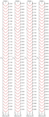 |
Fig. A.1. Observed line profiles (black dots) and their model fits (red lines) for the S1 Doppler reconstruction shown in Fig. 6. The phases of the individual observations are listed on the right side of the panels. |
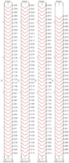 |
Fig. A.2. Same as in Fig. A.1, but for fitted line profiles for the S2 Doppler reconstruction shown in Fig. 6. |
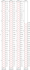 |
Fig. A.3. Same as in Fig. A.1, but for fitted line profiles for the S3 Doppler reconstruction shown in Fig. 8. |
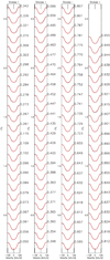 |
Fig. A.4. Same as in Fig. A.1, but for fitted line profiles for the S4 Doppler reconstruction shown in Fig. 8. |
All Tables
Adopted X-ray observations of V471 Tau with their durations and the quiescent periods within them.
Spectral fits to the quiescent parts of the two XMM-Newton observations from 2004 and 2019 and the Swift data from 2015.
All Figures
|
Fig. 1. Part of the Kepler K2 short-cadence data of V471 Tau with a particular flare event occurred when the white dwarf component was in eclipse. |
| In the text | |
|
Fig. 2. Spectral energy distribution for V471 Tau generated by the VOSA SED analyzer tool (Bayo et al. 2008). The synthetic spectrum (blue line) is fitted to the available archival photometry (red dots) from the Tycho, SLOAN/SDSS, Gaia DR2, 2MASS, AKARI/IRC, and WISE surveys. |
| In the text | |
|
Fig. 3. Variation in the surface temperature of the K2 star along the orbital phase. The dots show the temperature values derived individually for each spectra (blue for the 2005 season, red for the 2014–2015 spectra) by spectral synthesis. Open circles around zero phase correspond to those unaffected spectra that were observed when the white dwarf was eclipsed. The temperature rise of ≈100 K at ϕ ≈ 0.5 in both seasons may indicate the irradiation effect of the hot component (see Sect. 3.2 for details). |
| In the text | |
|
Fig. 4. K2 light curve of V471 Tau (top) and residual light variations (bottom) due to spots and flares after extracting the eclipsing binary model (see Sect. 4.1 for details). |
| In the text | |
|
Fig. 5. Cumulative flare-frequency diagram for V471 Tau. The slope of the linear fit (orange line) corresponds to α = 1.8 power-law index. |
| In the text | |
|
Fig. 6. Two Doppler images of V471 Tau from the 2005 data (S1 and S2). The surface temperature reconstructions are plotted in four rotational phases. |
| In the text | |
|
Fig. 7. Combined Doppler image of V471 Tau derived from all the available spectra from 2005 (S1+S2). The surface temperature map is plotted in four rotational phases. |
| In the text | |
|
Fig. 8. Two Doppler images of V471 Tau for the second observing run at the turn 2014–2015 (S3 and S4). The surface temperature reconstructions are plotted in four rotational phases. |
| In the text | |
|
Fig. 9. Combined Doppler image of V471 Tau derived from all the spectra in the second observing run at the turn 2014–2015 (S3+S4). The surface temperature map is plotted in four rotational phases. |
| In the text | |
|
Fig. 10. Average cross-correlation function map derived from the subsequent Doppler images plotted in Figs. 6 and 8. Black represents strong correlation, while light pink indicates no correlation. The quadratic sine fit (solid line) applied to the ridge of the correlation pattern (dots with error bars) suggests a solar-type rotational law with a very weak shear of αDR = 0.0026 ± 0.0006. See Sect. 5.3 for details. |
| In the text | |
|
Fig. 11. Dynamic Hα spectrum from the 2005 data (S1+S2). The individual 1D Hα spectra along the orbital phase are plotted in the rest frame of the K star. Dark green corresponds to deep absorption, while light yellow indicates strong emission. The large amplitude (≈320 km s−1) sine curve is the radial velocity of the white dwarf; the smaller amplitude (≈150 km s−1) sinusoid is the radial velocity of the centre of mass of the binary system. The tick marks on the right indicate the phases of the observations. |
| In the text | |
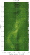 |
Fig. 12. Same as Fig. 11, but for the 2014–2015 data (S3+S4). |
| In the text | |
|
Fig. 13. Evolution of the X-ray luminosity of the K dwarf in V471 Tau from the observations summarized in Table 1. The duration of the selected quiescent ranges is color-coded. Solid error bars denote flux errors (see text); dotted bars are the estimated cross-calibration uncertainty. The blue dashed line indicates the best fit with a sinusoidal function with a period of ∼12.7 yr. |
| In the text | |
|
Fig. 14. Flare duration vs. flare energy from the K2 data of V471 Tau. The best fit indicates a power-law relationship with 0.5 ± 0.02 index. |
| In the text | |
|
Fig. A.1. Observed line profiles (black dots) and their model fits (red lines) for the S1 Doppler reconstruction shown in Fig. 6. The phases of the individual observations are listed on the right side of the panels. |
| In the text | |
|
Fig. A.2. Same as in Fig. A.1, but for fitted line profiles for the S2 Doppler reconstruction shown in Fig. 6. |
| In the text | |
|
Fig. A.3. Same as in Fig. A.1, but for fitted line profiles for the S3 Doppler reconstruction shown in Fig. 8. |
| In the text | |
|
Fig. A.4. Same as in Fig. A.1, but for fitted line profiles for the S4 Doppler reconstruction shown in Fig. 8. |
| In the text | |
Current usage metrics show cumulative count of Article Views (full-text article views including HTML views, PDF and ePub downloads, according to the available data) and Abstracts Views on Vision4Press platform.
Data correspond to usage on the plateform after 2015. The current usage metrics is available 48-96 hours after online publication and is updated daily on week days.
Initial download of the metrics may take a while.