| Issue |
A&A
Volume 650, June 2021
|
|
|---|---|---|
| Article Number | A156 | |
| Number of page(s) | 18 | |
| Section | Galactic structure, stellar clusters and populations | |
| DOI | https://doi.org/10.1051/0004-6361/202040065 | |
| Published online | 24 June 2021 | |
Clustered star formation toward Berkeley 87/ON2
I. Multiwavelength census and the population overlap problem⋆
1
Departamento de Física, Ingeniería de Sistemas y Teoría de la Señal, Universidad de Alicante, Carretera de San Vicente s/n, 03690 San Vicente del Raspeig, Alicante, Spain
e-mail: This email address is being protected from spambots. You need JavaScript enabled to view it.
2
Departamento de Astrofísica, Centro de Astrobiología (CSIC-INTA), Ctra. Torrejón a Ajalvir km 4, 28850 Torrejón de Ardoz, Spain
3
Instituto de Astronomía, Unidad Académica de Ensenada, Universidad Nacional Autónoma de México, Ensenada 22860, Mexico
4
Institute for Astrophysics, University of Vienna, Türkenschanzstrasse 17, 1180 Vienna, Austria
Received:
4
December
2020
Accepted:
8
March
2021
Abstract
Context. Disentangling line-of-sight alignments of young stellar populations is crucial for observational studies of star-forming complexes. This task is particularly problematic in a Cygnus-X subregion where several components, located at different distances, overlap: the Berkeley 87 young massive cluster, the poorly known [DB2001] Cl05 embedded cluster, and the ON2 star-forming complex, which in turn is composed of several H II regions.
Aims. We provide a methodology for building an exhaustive census of young objects that can consistently treat large differences in extinction and distance.
Methods. OMEGA2000 near-infrared observations of the Berkeley 87/ON2 field were merged with archival data from Gaia, Chandra, Spitzer, and Herschel and with cross-identifications from the literature. To address the incompleteness effects and selection biases that arise from the line-of-sight overlap, we adapted existing methods for extinction estimation and young object classification. We also defined the intrinsic reddening index, Rint, a new tool for separating intrinsically red sources from those whose infrared color excess is caused by extinction. Finally, we introduce a new method for finding young stellar objects based on Rint.
Results. We find 571 objects whose classification is related to recent or ongoing star formation. Together with other point sources with individual estimates of distance or extinction, we compile a catalog of 3005 objects to be used for further membership work. A new distance for Berkeley 87, (1673 ± 17) pc, is estimated as a median of 13 spectroscopic members with accurate Gaia EDR3 parallaxes.
Conclusions. The flexibility of our approach, especially regarding the Rint definition, allows overcoming photometric biases caused by large variations in extinction and distance in order to obtain homogeneous catalogs of young sources. The multiwavelength census that results from applying our methods to the Berkeley 87/ON2 field will serve as a basis for disentangling the overlapped populations.
Key words: methods: observational / techniques: photometric / catalogs / open clusters and associations: individual: Berkeley 87 / ISM: individual objects: ON2 / stars: formation
Full Tables 2 and C.1 are only available at the CDS via anonymous ftp to cdsarc.u-strasbg.fr (130.79.128.5) or via http://cdsarc.u-strasbg.fr/viz-bin/cat/J/A+A/650/A156
© ESO 2021
1. Introduction
The closest giant star-forming complex, Cygnus-X, is a privileged site in which to observe the conditions under which massive star clusters are born and mature. The rich variety of star-forming clouds, OB clusters, and associations that are part of Cygnus-X (Le Duigou & Knödlseder 2002; Reipurth & Schneider 2008) is ideal for understanding how feedback from massive stars affects the formation of new clusters in the surroundings. To assess this interplay between components, it is crucial to know the three-dimensional structure of the complex precisely. In other words, the young populations that overlap along the line of sight must be disentangled.
Measuring distances toward Cygnus-X is a challenging task, however. The complex is located in a kinematic avoidance zone (Ellsworth-Bowers et al. 2015), where the line of sight is nearly tangential to the Galactic rotation. This implies that kinematic distances are highly uncertain up to several kiloparsecs, to the point that deciding whether Cygnus-X components are physically connected or if their distances are not even comparable has been a long-standing controversy (Pipenbrink & Wendker 1988; Uyanıker et al. 2001; Schneider et al. 2006; Rygl et al. 2012).
With the advent of the Gaia mission (Gaia Collaboration 2016), the line-of-sight overlap problem can be partially solved. Gaia parallaxes yield accurate distance results for optically visible stellar populations in Cygnus-X (Berlanas et al. 2019; Lim et al. 2019). Distances to dust clouds can also be derived from Gaia parallaxes if reddened stars located behind them are still detectable in optical wavelengths (Zucker et al. 2019, 2020; Alves et al. 2020). These techniques are no longer valid under heavier extinction conditions, however, and they are not applicable to individual point sources that are only detectable in longer wavelengths (e.g., masers, protostars).
In this series of papers, we study a particularly troublesome subregion in southwestern Cygnus-X, where several components are projected onto the same field. The most relevant objects related with clustered star formation are introduced below (and shown in Fig. 1).
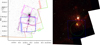 |
Fig. 1. Left: spatial coverage of the OMEGA2000, Chandra, and IRAC observations in the 3.6 μm image of the ON2 region. Right: RGB image (R = [8.0],G = [4.5],B = [3.6]) of the region that is covered by coordinate axes in the left panel, and showing the OMEGA2000 field of view in the same way. Green circles show the position and size of Berkeley 87 (dashed) and [DB2001] Cl05 according to Dias et al. (2014) and Dutra & Bica (2001), respectively. The Cygnus 2N region is marked as a yellow diamond. |
Berkeley 87 is a young massive cluster, located ∼1.7 kpc away. It is famous for hosting massive stars in rare phases of their late evolution, such as the peculiar emission-line variable V439 Cyg (Polcaro et al. 1989; Polcaro & Norci 1998). It is also the only cluster in the Milky Way that is currently known to host an oxygen-rich Wolf-Rayet (WR) star, WR 142 (Barlow & Hummer 1982; Drew et al. 2004; Oskinova et al. 2009; Rate et al. 2020). The first complete characterization of Berkeley 87 was carried out by Turner & Forbes (1982), and further studies were presented by Polcaro et al. (1991), Massey et al. (2001), Turner et al. (2006), Bhavya et al. (2007), Majaess et al. (2008), Sokal et al. (2010), and Oskinova et al. (2010).
ON21 is a star-forming complex whose southern half, ON 2S, is projected close to the center of Berkeley 87. The main components of ON 2S are the G75.77+0.34 H II region and the Cygnus 2N site of massive star formation. The latter hosts several water masers whose distances have been measured by Ando et al. (2011), Xu et al. (2013), and Moscadelli et al. (2019) through trigonometric parallaxes, yielding (3.83 ± 0.13) kpc,  , and (3.72 ± 0.43) kpc, respectively.
[DB2001] Cl05 is an infrared star cluster that seems to be embedded in the G75.77+0.34 cloud. The overdensity of reddened stars was discovered independently by two teams, Dutra & Bica (2001) and Comerón & Torra (2001). While the former simply claimed that this cluster is “related to OH maser ON2, background of cluster Be87” without further explanation, the latter discussed ON2, Berkeley 87 and [DB2001] Cl05 as part of the same complex. No additional research on the embedded cluster was published until Skinner et al. (2019) detected X-ray emission from several of the reddened stars. These authors assumed the same distance as the aligned water masers measured by Xu et al. (2013), 3.5 kpc.
To characterize a young cluster or star-forming region, it is common practice to measure properties such as extinction and distance to one or a few components and then apply the results to the whole system. This simplification often works well because alignments of cluster-forming regions are infrequent, but this is not the case for the ON2 line of sight. Nevertheless, several works on Berkeley 87 and ON2 have proceeded in this way (Giovannelli 2002; Bhavya et al. 2007; Oskinova et al. 2010; Binder & Povich 2018) to obtain results or elaborate discussions that would be called into question if new distances were taken into account. Even though Skinner et al. (2019) correctly pointed out the incompatible distances for Berkeley 87 and ON2, their implicit assumption that [DB2001] Cl05 is physically connected to the aligned masers is still unproven.
In this first paper, we address the line-of-sight overlap problem through a new approach that treats large distance and extinction ranges in a consistent way. The intended outcome is a multiwavelength census of objects potentially belonging to one of the overlapping young populations.
2. Observations and data reduction
This research makes use of deep imaging and photometry from various instruments whose spatial coverages (excluding all-sky surveys) are shown in Fig. 1. Raw observations that were specifically reduced for this work (Sects. 2.1 and 2.2) are complemented with fully calibrated data that were made publicly available by other teams (Sects. 2.3 and 2.4). In Sect. 2.5 the results are merged into a multiwavelength point-source catalog whose astrometry is recalibrated with the Early Data Release 3 (EDR3) of Gaia (Gaia Collaboration 2021).
2.1. Near-infrared
The 15′ × 15′ field described above, centered at α = 20h21m45.1s; δ = +37° 21′42″, was observed on July 7, 2009, with the OMEGA2000 camera mounted on the 3.5-m telescope of the Calar Alto Observatory, Spain. J-, H-, and K-band images were obtained with seeing full width at half maximum (FWHM) values of 1.11, 1.23, and 1.15 arcsec, respectively.
The near-infrared images from the OMEGA 2000 camera were processed with a modified version of the FLAMINGOS pipelines (Levine 2006; Román-Zúñiga 2006). These pipelines are based on IRAF/Fortran and IDL scripts. A first pipeline is used to reduce the raw data through a process that includes instrumental signal subtraction, illumination correction, and two passes of sky subtraction before applying a combination of the dithered exposures into a mosaic by means of an optimized centroid determination. Then a second pipeline provides identification and extraction of most sources present in the combined mosaics using the SExtractor algorithm (Bertin & Arnouts 1996) with a Gaussian filter and a 64-level deblending. Then, point-spread function (PSF) and aperture photometry are performed on all the detected sources using IRAF/DAOPHOT. An astrometric solution is provided by cross matching with Two Micron All-Sky Survey (2MASS; Skrutskie et al. 2006) catalogs of the same observed region. For this dataset, we confirmed that the PSF photometry has significantly better quality than the aperture photometry measurements, which is mostly due to source crowding. Therefore we decided to discard the aperture-based magnitudes. Finally, we used the TOPCAT software (Taylor 2005) for astrometric matching of the J-, H-, and K-band PSF catalogs (and for subsequent catalog matches in this work); a 0.75″ tolerance for the sky position error was carefully chosen because higher separations mainly produced spurious coincidences in regions of high stellar density.
The resulting source list was matched against the 2MASS and UKIDSS (UKIRT Infrared Deep Sky Survey; Lawrence et al. 2007) catalogs for photometric calibration purposes. We performed a comparative analysis, based on which we prefer calibrating with the UKIDSS wide field camera (WFCAM) photometric system (Hewett et al. 2006) for the following reasons. First, the OMEGA2000 and UKIDSS K bandpasses are quite similar2, while the 2MASS KS filter lacks the longest wavelengths (≳2.3 μm), making equivalences more problematic. Second, UKIDSS covers a broader dynamic range, as displayed in the calibration diagrams (Fig. 2a). Third, the lower dispersion of UKIDSS calibration allows a more accurate zeropoint determination. This lower dispersion enables the detection of a weak bimodality in the J-band zeropoint (ΔJZP ∼ 0.07; Fig. 2c) that would not be noticed in the 2MASS calibration. We discovered that the bimodality is spatially correlated with the circular shape of a high-illumination artifact (Fig. 2b) in the OMEGA2000 J-band flat-field image. We solved this issue by setting two different zeropoints in the appropriate regions. Finally, all the zeropoints in the three bands were applied after any significant color terms were discarded.
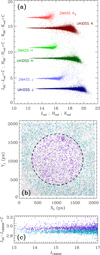 |
Fig. 2. Photometric calibration of OMEGA2000 (“O2”) data. Panel a: comparison of calibration diagrams using 2MASS or UKIDSS as the reference (“ref”) survey. Panel b: location of J-band point sources (colored crosses: JUKIDSS < 17; σJ < 0.035) relative to the flat-field artifact, see Sect. 2.1. Panel c: close-up view of panel a showing the J-band bimodality; symbols are as in panel b. |
For bright sources with saturation or nonlinearity problems (specifically, J < 13.50; H < 12.65; K < 12.25 in the OMEGA2000 field, and J < 11.5; H < 12.04; K = 10.5 in the control field), 2MASS photometry was used instead. The 2MASS magnitudes were converted into the WFCAM photometric system according to the Hodgkin et al. (2009) transformations.
2.2. X-rays
X-ray data of the Berkeley 87/ON2S region were obtained with the Advanced CCD Imaging Spectrometer (ACIS) onboard the Chandra X-ray Observatory in two different epochs: February 2, 2009 (ObsID: 9914; PI: Skinner), and August 13, 2016 (ObsID: 18083; PI: Skinner). The ACIS-I configuration was used, and the net exposure times were 70.15 and 69.07 ks, respectively. Results for these observations have only been published in a partial way: Sokal et al. (2010) and Skinner et al. (2019) analyzed only a limited number of X-ray sources in the field, while Townsley et al. (2019) published an exhaustive catalog, but for the 2009 observation alone. Therefore we carried out our own reduction of both epochs. This produced a homogeneous list of sources in the overlapping region (which includes the [DB2001] Cl05 cluster; see Fig. 1). The raw data were downloaded from the Chandra Data Archive and were processed with version 4.9 of the Chandra Interactive Analysis of Observations (CIAO) software (Fruscione et al. 2006), following the steps listed below.
For each dataset, we obtained a level-2 event file with updated calibration files using the chandra_repro script. Then, images in the broad (0.5–7 keV), soft (0.5–1.2 keV), medium (1.2–2 keV), and hard (2–7 keV) energy bands were extracted for binning factors of 1, 2, and 4 pixels through the fluximage tool. The PSF, which varies strongly throughout the ACIS-I field of view due to geometric distortion, was computed with mkpsfmap for each broadband image, choosing standard values for the enclosed count fraction, 0.393, and monochromatic energy, 1.49 keV. The next step consisted of detecting sources in the broadband images through the wavdetect algorithm (Freeman et al. 2002), taking wavelet scales of 1, 2, 4, 8 and 16 pixels.
The use of three different binning factors is intended to optimize the astrometric accuracy, which is crucial for counterpart identification in such a crowded field. The optimal binning factor for source extraction was decided on a case-by-case basis, as illustrated in Fig. 3. In general, the 1-pixel binning performs better in crowded regions or bright sources, and higher binning factors are preferable near the edges of the ACIS-I field (which are severely affected by geometric distortion).
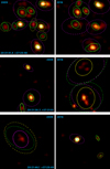 |
Fig. 3. Comparison of X-ray detection ellipses in three 40″ × 40″ closeups, centered at the coordinates that are printed in blue, of the 2009 (left) and 2016 (right) Chandra/ACIS fields, using binning factors of 1 (green), 2 (yellow), and 4 (purple) pixels. Ellipses that were selected for the final source list are drawn with solid lines. The background images are 2-pixel binned. Upper panels: portion of the [DB2001] Cl05 cluster, middle panels: region near the edge of the 2016 field, and lower panels: region near the 2009 edge. |
When the sources were extracted for the 2009 and 2016 fields, the two respective source lists were spatially matched, allowing for a maximum uncertainty of 4″. This value was chosen as a compromise between source separations in the densest regions (e.g., in the upper panels of Fig. 3) and the position errors of Chandra catalog sources that were measured by (Rots & Budavári 2011, see their Fig. 4) for large off-axis angles. In the process, we detected that the 2016 field was shifted by Δα ≈ 0.46″; Δδ ≈ 0.30″ relative to the 2009 epoch, which in turn is better aligned with the OMEGA2000 astrometry. This shift was corrected for so that both epochs are spatially matched.
The final source list contains a total of 247 point sources within the 15′ × 15′ OMEGA2000 field, 54 of which are detected in both epochs. For these common sources, we assigned the coordinates of the smallest detection ellipse.
We note that the small number of two-epoch detections should not be interpreted in terms of variability. On the one hand, the two ACIS fields overlap only in part: the solid angle in common covers 45% of our near-infrared field of view (see Fig. 1). On the other hand, detection depends strongly on geometric distortion, which can change dramatically between epochs for the same object, as explained above and shown in Fig. 3 (especially in the middle and lower panels). Unfortunately, distinguishing between actual variability and distortion as the cause of a nondetection would require an analysis of upper limits. This is beyond the scope of this paper.
We defer a determination of X-ray fluxes to the second paper of this series. Comprehensive results for extinction from infrared counterparts will then allow us to obtain intrinsic fluxes.
2.3. Mid-infrared
Mid-infrared images and the photometric catalog were downloaded from the website of the Cygnus-X Spitzer Legacy Survey project3. The survey catalog includes the 3.6, 4.5, 5.8 and 8.0 μm bands of the Infrared Array Camera (IRAC) and the 24 μm band of the Multiband Imaging Photometer for Spitzer (MIPS).
Because Berkeley 87 is located near a corner of the surveyed region, the spatial coverage of our 15′ × 15′ field of interest is partial in some Spitzer bands. Specifically, the southwestern corner of the OMEGA2000 field was excluded from the 4.5 and 8.0 μm observations (see Fig. 1). We did not include the MIPS observations because they only cover a small portion of the near-infrared field, around its northeastern corner.
2.4. Far-infrared
The ON2 region was observed by the Herschel Space Observatory (Pilbratt et al. 2010) on April 11, 2012 (observation IDs: 1342244190 and 1342244191; PI: Molinari), and April 12, 2012 (observation IDs: 1342244166 and 1342244167; PI: Molinari). These observations were carried out in parallel mode, producing simultaneous scans at the 70 μm and 160 μm bands of the Photodetector Array Camera and Spectrometer (PACS; Poglitsch et al. 2010), and the 250 μm, 350 μm, and 500 μm bands of the Spectral and Photometric Imaging Receiver (SPIRE Griffin et al. 2010). Because of the ∼21′ shift between the PACS and SPIRE pointings in parallel mode, the spatial coverage was complete only for the April 11 SPIRE map and for the April 12 PACS image. We therefore only employed this combination of observations. The four level-2.5 calibrated maps (one for each instrument and each date) and the corresponding point-source catalogs (only available for the PACS bands) were downloaded from the Herschel Science Archive4.
2.5. Multiwavelength merging and astrometric recalibration
In a first attempt of spatial matching of the OMEGA2000 and Spitzer sources, we detected an enhanced dispersion in the RA direction, together with an average offset of 0.38″ to the west. After correcting for the offset, we matched both catalogs within a box, σα = ±1.2″; σδ = ±0.75″, which takes the anisotropic dispersion into account. Because our near-infrared data have a better resolution, the OMEGA2000 coordinates were chosen for the objects in common.
After the near- and mid-infrared catalogs were joined, the Gaia EDR3 catalog was downloaded from the Gaia archive5. Gaia counterparts for our infrared point sources were searched for in a radius of 0.75″, consistently with previous position matches. The median values αIR − αGaia = 0.103″ and δIR − δGaia = 0.162″ were used for the recalibration; the respective standard deviations, 54 mas and 76 mas, prove the excellent performance of the OMEGA2000 relative astrometry.
Merging the resulting catalog with the Chandra and Herschel data was not straightforward owing to astrometric uncertainties that exceed the typical angular separations between near-infrared point sources. The Chandra case is particularly problematic because the astrometric accuracy strongly changes with the position within the field of view.
Figure 4 shows angular distances (θ) between Chandra sources and data points from the infrared catalog. In principle, the gray histogram would lead us to interpret the minimum at ∼1″ as a clear transition between genuine and spurious coincidences. However, examination of X-ray sources whose closest neighbor separations are θnearest > 1″ revealed that the longer θnearest, the larger the detection ellipse, up to a limit of θnearest = 2.0″. This entails that real counterparts are still likely to be found within this range due to variable distortion. Consequently, θnearest ≤ 1″ infrared counterparts are classified as likely, provided that no additional source is present in θ ≤ 2″. The remaining X-ray sources fulfilling θ ≤ 2″ were addressed on a case-by-case basis using the following criteria: position and size of the detection ellipse relative to the location of the candidate counterpart; position of the secondary X-ray detection (i.e., in the alternative epoch), if any; or mid-infrared brightness. Two hundred infrared sources were selected as likely counterparts of Chandra sources, and 24 were marked as doubtful. We were unable to determine any counterpart for the remaining 23 X-ray sources located within the 15′ × 15′ near-infrared field.
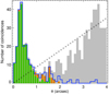 |
Fig. 4. Histogram of angular separations between X-ray and infrared point sources (after absolute astrometric calibration with Gaia). Gray bars include all coincidences, and the blue line only accounts for the nearest infrared neighbor of each X-ray source. Green bars are the number of infrared sources that were finally accepted as counterparts, and the orange portions were marked as doubtful. As a reference, black crosses show the case of a random source distribution (indicative of a case in which all coincidences are spurious). |
Regarding Herschel, the 70 μm and 160 μm catalogs were matched with maximum angular separations of 5″. All 70 μm detections were searched for counterparts in the [5.8] or [8.0] Spitzer bands within a 4″ radius. Because only nine Spitzer counterparts were found, all of them were inspected. All these far- to mid-infrared matches were finally kept as positive, except for one Herschel source that is compatible with the Cygnus 2N compact H II region. This special case is separately discussed in Sect. 2.6 because of its relevance as a distance estimator for the ON2 region.
The final multiwavelength list of sources contains 47 090 objects in total. In order to provide cross-identifications from the literature, coordinates of previously studied objects were obtained from the SIMBAD6 database (Wenger et al. 2000) and matched with our combined source list with a 1″ tolerance. These include 19 stars of known spectral type, which are listed in Table 1. Finally, identifiers from the recent X-ray catalog by Skinner et al. (2019) were also added to our catalog by matching their coordinates in a 1″ radius.
Stars of known spectral type in the OMEGA2000 field.
2.6. Cygnus 2N region
Figure 5 displays multiwavelength source positions over a K-band image of the Cygnus 2N H II region and its surroundings. The brightest PACS point source in the ON2 region (f70 μm = 2066 Jy; f160 μm = 2127 Jy) appears to be coincident with the Cygnus 2N radio continuum source (Matthews et al. 1973; Harris 1974), which in turn is subdivided into three compact sources of different evolutionary state (Sánchez-Monge et al. 2013; Cho et al. 2016). Furthermore, three Spitzer sources with very red colors (one of them is coincident with the EAST ultracompact H II region, as already noted by Sánchez-Monge et al. 2013) are located very close to the far-infrared peak. All of them form a structure that is elongated in the same direction as the Herschel source, as shown with the red contours in Fig. 5. This geometry might indicate that far-infrared radiation in this small region comes from a group of objects that are not resolved by Herschel. In any case, the uncertainty of the 70 μm detection is larger than the separations between the point sources in Fig. 5, as revealed by the discrepancy between the peak position and the PSF-fitted coordinates (see Marton et al. 2017) from the PACS catalog. Likewise, the Chandra detection in the central part of Fig. 5 could also be related to various objects belonging to the Cygnus 2N star-forming region based on the extended size of the detection ellipse, which encompasses multiple infrared sources.
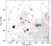 |
Fig. 5. OMEGA2000 K-band image (grayscale) and point-source catalog (small blue crosses) of the Cygnus 2N region. The Herschel/PACS 70 μm map is overplotted as contours with an interval of 3.5 Jy arcsec−2; the positions of the 70 μm and 160 μm detections according to the Herschel public catalog are marked as orange and red circles, respectively. Chandra detection ellipses are drawn as dashed blue lines, and infrared sources detected by Spitzer at wavelengths larger than 5 μm are shown as large pink crosses. The remaining symbols indicate objects reported by Sánchez-Monge et al. (2013): green and turquoise pluses are methanol and water masers, respectively, and purple squares are the centimeter continuum sources that were called CORE (C), EAST (E), and UCHII (U) by these authors. |
These arguments led us to consider both the Herschel and Chandra detections as counterparts of the whole Cygnus 2N H II region. The closest mid-infrared source, which was initially matched with the Herschel source, is now considered as a different catalog entry that matches the EAST object.
Nevertheless, a caveat about the Cygnus 2N X-ray counterpart must be added: This faint source is only detected by wavdetect in the 4-pixel binned image of the 2016 observation, where this source is placed at the edge of the gap between the ACIS-I detectors. We therefore cannot discard that this detection is caused by a reduction artifact. Still, coincidence with the Cygnus 2N region indicates that this Chandra source is real because X-ray emission is commonly associated with regions of massive star formation (Townsley et al. 2014, 2018).
3. Basic observational features and practical definitions
In a first inspection of the multiwavelength data (e.g., images and photometry in Fig. 6, which are discussed below in more detail), we find the following observational features that indicate a superposition of components. First, Berkeley 87 known members (a total of 15) appear to be among the least reddened point sources, implying that valuable information can be provided by Gaia. Second, a conspicuous concentration of very reddened objects toward the [DB2001] Cl05 region can only be detected at X-ray and infrared wavelengths. Based on these features, we provide some practical definitions below to isolate different populations.
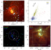 |
Fig. 6. Multiwavelength RGB images (colored as indicated in the upper left corner of each image) of the Berkeley 87/ON2 region, and infrared color–color diagram of the OMEGA2000 field. The extinction vector that is shown in this diagram (panel b) is obtained from Indebetouw et al. (2005), and taking AK/AKS ≈ 0.98 (which is justified in Appendix A). In all the images, the Cl05 region is enclosed by a white or black circle. In the Herschel RGB image (d), the OMEGA2000 field coverage is shown as a white square. An infrared closeup of this field, centered on [DB2001] Cl05, is displayed in panel a, and its Chandra counterpart is shown in panel c. The latter is made of 2-pixel binned images from the 2009 observation; the density of J − H > 1.7 sources is drawn as gray contours (dotted = 55 arcmin−2; dashed = 110 arcmin−2). In all panels, Berkeley 87 spectroscopic members are marked as open blue diamonds, except for WR 142, which is shown as an open blue circle (only in panels b and d); crosses are point sources within the Cl05 region that are simultaneously detected in J, H, K, and [5.8] (i.e., those that are represented in panel b). |
3.1. Preliminary components
Isocontours enclosing sources of increasing J − H colors revealed a conspicuous overdensity of very red (J − H > 1.7) point sources around the position of the [DB2001] Cl05 cluster. Figure 6c shows that this overdensity (gray contours) is roughly coincident with the group of X-ray point sources in the G75.77+0.34 H II region that was previously reported by Skinner et al. (2019). Based on this spatial distribution, we define the “Cl05 region” as the circle of radius 75 arcsec centered at α = 305.414; δ = 37.436 (which is drawn in all RGB images in Fig. 6) to serve as a rough, preliminary delimitation of the embedded cluster. We remark that this definition has merely practical purposes (e.g., to compare point-source properties inside and outside the overdensity) and is not aimed at anticipating any properties of the cluster.
Another striking observational feature of the field is a bimodality in the JHK colors that is clearly visible in color–color diagrams (Fig. 6b and others in Fig. A.1). Because near-infrared color excesses (especially in the J − H case) are mainly affected by extinction (in contrast to the mid-infrared, where intrinsic reddening becomes stronger; see, e.g., Gutermuth et al. 2008; Teixeira et al. 2012), this bimodality may be interpreted as two extinction groups approximately separated by the minimum of the distribution J − H ≈ 1.35, or H − K ≈ 0.65. Hence, we define the low-reddening population (LRP) as composed of J − H ≤ 1.35 sources, or as H − K ≤ 0.65 for those lacking J-band detection. Likewise, we define the high-reddening population (HRP) as meeting J − H > 1.35, or H − K > 0.65 if J is missing.
Preliminarily, Fig. 6 provides evidence that the apparent cluster pair is just a chance alignment of unrelated star formation events. The color–color diagram in panel b reveals a large gap along the extinction vector between Berkeley 87 members (all of which belong to the LRP) and HRP sources located within the Cl05 region. The latter show particularly high K − [5.8] colors, favoring very young ages (see, e.g., Teixeira et al. 2012) for [DB2001] Cl05, in contrast to the Berkeley 87 cluster. Moreover, the distribution of hot dust (bluer colors on the Herschel image in panel d) appears to be spatially compatible with the Cl05 region and incompatible with the projected distribution of hot massive Berkeley 87 members despite the well-known feedback power of this type of stars. The case of WR 142 is especially meaningful because this extremely hot star and its mighty wind (Tramper et al. 2015; Sander et al. 2019) show no heating effects on the aligned dust that is detected by Herschel; this lack of hot matter suggests a distance discrepancy between Berkeley 87 and ON2.
3.2. Intrinsic reddening
We need to distinguish here between intrinsic and interstellar color excess for two main reasons. First, breaking this degeneracy is crucial to correctly estimate interstellar extinction toward each star, especially when only photometric information is available. Second, we aim at finding populations of young stellar objects (YSOs), which are commonly revealed as intrinsically red sources. Although other photometric methods for YSO discovery and classification, based on color excess, have been developed before (e.g., Lada et al. 2006; Gutermuth et al. 2009), these methods require an extensive wavelength coverage in the mid-infrared that is not fulfilled in the Cl05 region. For example, few JHK sources are also detected in [5.8] within this region (pink crosses in Fig. 6). Therefore the incompleteness of near-infrared data demands a more flexible treatment.
Because reddening is dominated by interstellar extinction toward shorter infrared wavelengths (see, e.g., Indebetouw et al. 2005), color-color diagrams that combine one long-wavelength color X = X2 − X1 and one short-wavelength color Y = Y2 − Y1 (e.g., Fig. 6b) are useful for determining the origin of infrared color excess. We specifically refer to (X, Y) diagrams where the X color encompasses K-band wavelengths and longer, and the Y color is part of the JHK range. As shown by Teixeira et al. (2012), these diagrams place most of stars on the main sequence and its interstellar reddening band, while intrinsically red sources are clearly shifted to redder X colors. Based on this idea, we propose measuring intrinsic reddening of each object as a weighted average of the X excesses that are measured in the (X, Y) diagrams where the source is present. Thus, we define the intrinsic reddening index, Rint, as
 (1)
(1)
where each SX, Y is the relative shift along the X direction from the reddening band boundary of each diagram, and WX, Y is the respective weight. The complete definitions of SX, Y, WX, Y, and the reddening band boundaries are presented in Appendix A, together with a discussion of which X and Y colors are included (or excluded). The six resulting color–color diagrams that are finally involved in the Rint calculation are displayed in Fig. A.1.
4. Extinction and distance
This section is aimed at measuring extinction and distance for as many objects as possible in our merged photometric catalog. Because of the unusually complex nature of the field, in which multiple stellar populations are located at different distances, several methods of extinction estimation are combined. On the one hand, we employ intrinsic colors of relatively nearby stars when this information can be obtained either directly or indirectly from the literature. On the other hand, we estimate extinction for a much larger sample by applying the Majewski et al. (2011) method to our photometric data.
4.1. Extinction from individual estimates of intrinsic color
First of all, we address extinction estimation for the stars whose intrinsic colors can be inferred directly from their known spectral types. All of the 19 stars in the catalog with previously published spectra are saturated in the OMEGA2000 images, therefore 2MASS photometry is used instead. Moreover, we take advantage of the V-band photometry published by Turner & Forbes (1982), which includes all these 19 objects.
In general, we relied on the intrinsic colors published by Ducati et al. (2001) for normal stars later than O9 I or B0 V. This is not applicable to the following exceptions: the O8.5-9 III-V star BD+36°4032, for which we used Martins & Plez (2006), and the special cases of WR 142 and V439 Cyg that are addressed separately. Because the two cited works employ the Johnson-Glass photometric system for the near-infrared (Bessell & Brett 1988), intrinsic colors were converted into the 2MASS system through the Carpenter (2001) transformations. For stars earlier than F, we used V − KS to obtain color excess (EV − KS), as its relative uncertainty is the lowest because of the extended wavelength range and because AKS ≪ AV (this makes the result less dependent on the chosen extinction law). For late-type stars, computing EV − KS is no longer appropriate because the uncertainties on intrinsic colors (see, e.g., V − K variations between adjacent spectral subtypes in Ducati et al. 2001) become comparable to the resulting color excess values; in these cases, J − KS was used instead.
The color excess for WR 142 and V439 Cyg cannot be accurately determined in the same way. In the former case, the reason is the lack of knowledge about intrinsic colors for WO stars, which are extremely rare. In the latter case, the strong photometric and spectroscopic variability of this object (Polcaro et al. 1989; Polcaro & Norci 1998) would require simultaneous photometry and spectroscopy. We therefore preferred to adopt the EB − V(V439 Cyg) = 1.53 value that Turner & Forbes (1982) obtained from color excesses of nearby Berkeley 87 members. Likewise, we assigned WR 142 the color excess EV − KS = 3.30 that we computed for an angularly close cluster member, TYC 2684-133-1.
Turner & Forbes (1982) estimated EB − V for 19 additional objects of unknown spectra by assuming that they are B-type stars in the Berkeley 87 main sequence. This assumption in turn is based on the UBV color–color diagram published by these authors. We used these color excess data as well, even though some of them would be excluded later if their Gaia parallaxes are incompatible with the cluster.
After determining the color excesses for the objects collected above (38 in total), we calculated their extinction values as follows. First, AV was obtained for the 18 stars with EV − KS and EJ − KS values through the Rieke & Lebofsky (1985) extinction law, and the AK/AKS ≈ 0.98 correction (see Appendix A). Thirteen of these 18 objects correspond to confirmed B stars, which are the only secured members whose color excesses have been determined independently (unlike WR 142 or V439 Cyg, based on nearby stars). Therefore we took these 13 extinction results (all within the range 3.75 ≤ AV ≤ 5.57, with an average of  ) as representative of Berkeley 87. By dividing each AV result by the corresponding EB − V from Turner & Forbes (1982), we obtained
  and σRV = 0.11 for the sample of 13 confirmed B-type members. Finally, this new RV calibration was used to convert the remaining EB − V estimates (i.e., from V439 Cyg and the Turner & Forbes 1982 B-type candidates) into their visual extinction values.
4.2. Extinction from the RJCE method
Owing to the low number of extinction determinations so far and because nearly all of them are candidate Berkeley 87 members, a substantial extension of the extinction sample is required to separate components along the line of sight. For this purpose, we used the Rayleigh-Jeans Color Excess (RJCE) method, designed by Majewski et al. (2011). These authors provided an equation to compute AKS through H − [4.5] on the basis that the value of this color, (H − [4.5])int, is virtually the same for the majority of spectral types, with notable exceptions (e.g., KM dwarfs) that are discussed below. Because Majewski et al. (2011) employed the 2MASS H-band filter, we have adapted their equation to the OMEGA2000 filter through the appropriate calibration (Sect. 2.1),
![Mathematical equation: $$ \begin{aligned} A_{K_S} = 0.918\,(H_\mathrm{OMEGA2000} -[4.5]-0.13), \end{aligned} $$](/articles/aa/full_html/2021/06/aa40065-20/aa40065-20-eq5.gif) (2)
(2)
which was divided by 0.114 to obtain AV. The AK/AKS ≈ 0.98 correction is already included in this conversion factor.
We caution that the RJCE method is not to be applied for objects whose (H − [4.5])int may deviate significantly from the nominal value of the method (0.08 when H2MASS is employed; 0.13 according to our adapted version), however. The trivial case is the population that shows a significant intrinsic color excess in the mid-infrared, which is precisely what Rint is able to distinguish. We therefore only applied the RJCE method to objects fulfilling Rint ≤ 1.25.
According to Majewski et al. (2011), other objects with deviating (H − [4.5])int values are OB stars, which are bluer, and KM dwarfs, which are redder. This leads to  underestimations and overestimations, respectively. These cases can be excluded by isolating the stellar populations in which these objects are detectable and their extinction values can be measured by the RJCE method, as discussed below.
First, we focus on OB stars, which are rare outside massive or intermediate-mass young (≲108 yr) clusters or associations These objects may be present in the Cl05 region, where the extinction of virtually no HRP sources can be measured with the RJCE method (with the Rint ≤ 1.25 constraint). This lack of RJCE results is caused by a mixture of photometric incompleteness effects, such as those described in Sect. 3.2 and Appendix B.1, and the fact that [DB2001] Cl05 appears to be dominated by Rint > 1.25 objects. Therefore, we can concentrate our efforts on Berkeley 87 and its surroundings. Because the strongest color excess of a cluster member, EB − V = 1.9 (Turner & Forbes 1982), corresponds to AKS = 0.65 (by applying Rieke & Lebofsky 1985), we can safely assume that any underestimated  values for OB stars would be lower than 0.65 in any case. Consequently, we decided to discard all
  results below 0.65 as some of them may be underestimated due to their unidentified OB nature. Because the photometric uncertainty of the RJCE method,
  , is significant in some cases, we only kept results that fulfilled
 (3)
(3)
The low-luminosity KM main-sequence stars are only detectable when they are much closer than Berkeley 87 and extinction is much lower. This implies that Eq. (3) would only be fulfilled by KM dwarfs whose (H − [4.5])int color is too large to cause such an overestimate, in which case they would fail to meet the Rint ≤ 1.25 condition. The validity of this claim is evaluated in Sect. 4.3.3, taking advantage of the Gaia capabilities for measuring nearby unextinguished faint sources.
As a side effect, Eq. (3) excludes not only OB stars and KM dwarfs, but also any other sources that are little affected by extinction. Fortunately, such objects are easily detected by Gaia, which potentially provides data that are more useful for membership determination than extinction.
4.3. Gaia distances
Because of the nature of Gaia observations, parallax data are necessarily focused on populations that are observed under low or mild extinction conditions, such as Berkeley 87. For the purpose of separating populations along the line of sight, this allows Gaia parallaxes to play a role that is complementary to that of the extinction data from Sect. 4.2.
4.3.1. Parallax bias correction
Before proceeding with the distance estimation, we clarify how we treated the systematics of Gaia EDR3 parallaxes. Lindegren et al. (2021) provided a recipe to correct for the parallax bias through an approximate model, which consists of two separate functions for the five- and six-parameter (hereafter 6-p) astrometric solutions. This model is only valid for certain magnitude and color ranges; only 1830 out of 3280 sources with available EDR3 parallaxes in the OMEGA2000 field fall within these ranges.
First, we performed the bias correction for these 1830 objects through gaiadr3_zeropoint7, a Python3 implementation of the Lindegren et al. (2021) recipe. The resulting bias estimates, ϖ − ϖcorr (where ϖcorr is the bias-corrected parallax), are always negative, with average and median values −34 and −36 μas, respectively (cf. the global EDR3 values, −17 and −21 μas; Lindegren et al. 2021).
This evidence of asymetric bias suggests that at least a rough bias correction should also be applied to the remaining 1450 objects before estimating their distances. All these objects falling outside the validity ranges of the Lindegren et al. (2021) model correspond to 6-p astrometric solutions. Therefore the average of the above calculated bias estimates for the 6-p subset, −37 μas, is adopted as a zero-order correction and applied to the 1450 parallaxes.
4.3.2. Procedure for distance estimation
Following the recommendations of Astraatmadja & Bailer-Jones (2016) and Luri et al. (2018), we chose a Bayesian approach to produce distance estimates, using the exponentially decreasing space density (EDSD) prior (Bailer-Jones 2015). This prior employs a single adjustable parameter, the scale length L, and the mode of its probability distribution is equal to 2L. Because we aim at determining where each object is located relative to Berkeley 87, we opted to use a single value for L that makes the mode of the prior equal to a first estimate of the cluster distance, obtained through parallax inversion,
 (4)
(4)
where  is computed as the median of the 13 spectroscopically confirmed members with fractional uncertainties fϖ = σϖ/ϖ < 0.1. Higher fϖ values are avoided here because the parallax inversion becomes strongly biased as a distance estimator (Luri et al. 2018; Bailer-Jones et al. 2018). This yields
  and
and  .
.
We therefore set L = 836.5 pc in the TOPCAT implementation of the Bayesian estimator (which makes use of the EDSD prior) to obtain distance estimates (rest) from all the parallax measurements. Likewise, we computed the 15.87% and 84.13% quantiles (r16, r84) of the probability density function of the posterior. In this way, the confidence interval defined as [r16, r84] is comparable in terms of likelihood to the confidence interval used by Bailer-Jones et al. (2018); in both cases, the enclosed probability is 68.27%, the same as for a Gaussian distribution within a ±1σ interval centered at its maximum. The distance results for the 13 Berkeley 87 members have a median of rBe87 = (1673 ± 17) pc.
We avoided the regime of high fϖ values where the posterior is significantly affected by the prior choice because these values would yield distance results that are spuriously consistent with Berkeley 87. The transition from the data-dominated to the prior-dominated posterior occurs at fϖ ∼ 0.3−0.4 for the EDSD prior (Bailer-Jones 2015; Astraatmadja & Bailer-Jones 2016). Therefore a simple solution would be setting an fϖ threshold well below this transition, for example, fϖ ≤ 0.2. We need to ensure, however, that this constraint would not disregard any valuable results by confirming the produced confidence intervals, Δr = r84 − r16. In our catalog, data points fulfilling f ≈ 0.2 yield relative uncertainties Δr/rest ≈ 0.5, and we consider that any looser distance determinations would not be useful to our goals. Likewise, negative parallaxes (see Luri et al. 2018) can be safely discarded in our case because they always lead to Δr/rest > 0.5. Consequently, we decided to calculate distances only for parallaxes fulfilling 0 < fϖ ≤ 0.2.
Finally, we must add a caveat about the effect of our approach on the validity of the distance results. The procedure we described above is tailored to the scientific goals of this series of papers; in particular, distances are intended to be evaluated relative to the optically visible cluster (i.e., Berkeley 87). Conversely, if optimal calculations for absolute distances were required for other purposes, a more careful election of the scale length should be made. Nevertheless, our prior choice (Eq. (4)) is expected to have a minor effect on distance results provided that the permitted fϖ range is well inside the data-dominated regime.
4.3.3. Distance results vs. extinction
A total of 737 objects fulfill the fϖ requirement in the 15′ × 15′ OMEGA2000 field, 40 of which have a valid extinction estimate available. The latter are represented in Fig. 7, together with a cumulative histogram of all 737 distances, and the AV variation along the Berkeley 87 direction according to the Stilism 3D extinction map (Lallement et al. 2018). Our results are consistent with those from Stilism as long as we take into account that this map may underestimate extinction in directions crossing dense cloud cores (as cautioned before by Capitanio et al. 2017). The abrupt slopes at ∼1.0 and 1.35 kpc may be caused by this condition. The outliers near the upper left corner of Fig. 7 are discussed below.
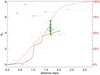 |
Fig. 7. Visual extinction vs. distance estimates, colored as follows: blue shows spectroscopically confirmed Berkeley 87 members, orange shows photometric candidates for Berkeley 87 membership according to Turner & Forbes (1982), magenta shows additional stars of known spectral types, black shows sources that were not previously cataloged, and gray is explained below. Objects whose AV values are obtained in Sects. 4.1 and 4.2 are shown as crosses and diamonds, respectively. The Berkeley 87 distance and AV range are represented as a green rectangle. The extinction along the Berkeley 87 direction according to the Stilism map is drawn as a solid black curve. The errors are shown as dotted lines. The dashed red curve is the cumulative distribution (see the scale on the right axis) for the sample of 737 objects with valid distance results, i.e., those that fulfill 0 < fϖ ≤ 0.2. The gray data point is not part of this sample and is only included to illustrate the effects of relaxing the fϖ constraints (see text). |
Figure 7 can be used to test the elimination of KM dwarfs from the results of the RJCE method, as explained in Sect. 4.2. If the conditions that exclude these nearby red objects (Rint > 1.25 and Eq. (3)) had been ignored, the region of Fig. 7 enclosed by AV > 5 and rest < 0.8 kpc would have been populated with 21 data points of clearly overestimated extinction. After applying the conditions, only two objects remain, and their results are close to the imposed limits (Rint = 1.13, 1.17, and  = 0.74 ± 0.05, 0.86 ± 0.08 for the objects located 367 and 690 pc away, respectively). This test shows that our decontamination of RJCE values is effective but not infallible.
The cumulative distribution shown in red in Fig. 7 illustrates that a great majority of the measured distances are comparable to or shorter than the Berkeley 87 distance. Furthermore, only one out of 737 distances corresponds to an HRP source, implying that Gaia EDR3 cannot be used for measuring populations as extinguished as [DB2001] Cl05 (see Sect. 3.1), at least with the required accuracy. Even if we had relaxed our fractional uncertainty condition up to fϖ = 0.3, we would have only found two HRP objects (one of those whose extinction could be estimated is shown as a gray symbol in Fig. 7), having no evidence of membership to any of the reddened components despite their far distances. These similarly bright objets (K ≈ 9.3) show HRP colors by a small margin (both have J − H ≈ 1.5, H − K ≈ 0.65) and are located angularly far (> 5′) from [DB2001] Cl05, showing no evidence of a young age (not detected by Chandra, Rint ≈ 0.7 for both). This illustrates the importance of complementing Gaia distances with extinction results to collect membership evidence throughout the line of sight.
4.3.4. Distance to Berkeley 87
Inspection of Fig. 7 also reveals that part of the photometric Berkeley 87 candidates listed by Turner & Forbes (1982) have Gaia EDR3 distances that are inconsistent with spectroscopic members. The obvious cases whose membership can be fully discarded are the foreground object Be87-54 ( ) and the background stars Be87-5, Be87-7, and Be87-95 (at
  , 2.02 ± 0.04, and
  , respectively). These three background objects might be part of another cluster or association because they share not only similar parallaxes, but also compatible proper motions.
Because at least some of the Turner & Forbes (1982) candidates are not Berkeley 87 members, we only used spectroscopically confirmed members to measure the distance to this cluster. We adopted the previously calculated median of 13 hot stars, rBe87 = (1673 ± 17) pc, which can be considered as our best distance estimate for Berkeley 87 because no distance results were obtained for any additional spectroscopic members. We note that only the statistical error of the median is considered here.
This result is in excellent agreement with the recent Gaia DR2 measurement of 1661 pc obtained by Cantat-Gaudin et al. (2018), although this result was computed from a different stellar sample and without taking spectral types into account. This agreement slightly contradicts the 1.75 kpc distance obtained by Skinner et al. (2019) as an average of only seven OB stars that were detected in X-rays by Sokal et al. (2010). All these Gaia-based results are located farther away than those from previous spectrophotometric studies in visible wavelengths (Turner & Forbes 1982; Turner et al. 2006, who obtained 0.95 and 1.23 kpc, respectively). This discrepancy is probably caused by a slightly overestimated extinction by Turner & Forbes (1982), who assumed RV = 3.0, while we obtain RV = 2.8 in Sect. 4.1.
5. Classification of young sources
5.1. Infrared selection of YSO candidates
To find and classify young sources through infrared photometry, the multiband YSO selection criteria by Gutermuth et al. (2008) and Gutermuth et al. (2009) (hereafter the G09 method) are commonly applied. This method was designed for a sample of nearby regions with little foreground extinction (in the most obscured cases, comparable to Berkeley 87), and generally located at relatively higher Galactic latitudes. However, the G09 method becomes problematic for observational conditions such as those in the ON2 field, which involve selection biases that jeopardize the efficacy of the method. An illustrative example is provided by the spatial distribution [5.8]-band counterparts of highly reddened JHK sources in the Cl05 region (pink crosses in Fig. 6). While some of these sources can be detected in relatively uncrowded regions displaying little extended emission, source confusion makes detection impossible in the densest most embedded regions. This is a serious hindrance for phase 1 of the G09 method, which requires simultaneous detection in all IRAC bands. To a lesser degree, this issue is still important in the [3.6] and [4.5] bands, which are simultaneously required for phase 2 of the G09 method.
A detailed characterization of selection biases affecting YSO selection in the infrared (including others that involve Galactic extinction and extragalactic contaminants) is provided in Appendix B. To overcome these biases and produce an acceptably homogeneous census of YSO candidates, we proceeded as follows. First, we applied phase 1 of the G09 method, but slightly adapted to the observational conditions of ON2. Second, our own method based on the Rint definition (Sect. 3.1 and Appendix A) was calibrated through results from the first step and was applied to the data instead of phase 2. Finally, supplementary YSO candidates were identified based on the far-infrared data.
5.1.1. IRAC-based selection
First of all, we tested phase 1, as originally published by Gutermuth et al. (2009), on the 15′ × 15′ OMEGA2000 field. This yielded 63 YSO candidates and 31 contaminants. Of the latter, 19 were categorized as extragalactic objects, 14 of which were classified as polycyclic aromatic hydrocarbon (PAH) galaxies, and 5 as broad-line active galactic nuclei (BL-AGN). However, the ratio of extragalactic contaminants to YSO candidates seems unrealistically high for a region with active clustered star formation in the Galactic plane, where extragalactic light is highly extinguished after crossing a long path through the Milky Way. A significant number of YSOs are indeed being misidentified as PAH or BL-AGN galaxies owing to magnitude cuts in the G09 method ([4.5]PAH < 11.5, and [4.5]BL-AGN < 13.5, respectively) that correspond to the YSO population in the nearest kiloparsec.
In order to correct these misidentifications, we modified the magnitude cuts described above as fully explained and justified in Appendix B.2. Briefly, the required adaption consists of changing the BL-AGN limit to one magnitude fainter ([4.5]> 14.5) and finding that only ∼0.64 PAH galaxies are expected in the OMEGA2000 field in the range 12.5 < [4.5] < 15, which is shared by YSOs. We consider this value low enough to simply ignore extragalactic contamination behind ON 2S. We adhered to the remaining steps of phase 1 (namely, removal of shock emission knots and PAH-contaminated apertures, selection of class 0/I candidates, and the same for class II), as in the original G09 method.
We note in the results that WR 142 and three Be-type members of Berkeley 87 (specifically, V439 Cyg, VES 203, and VES 204) are categorized as class II candidates. This is not entirely unexpected because Wolf-Rayet and Be stars commonly show strong mid-infrared excesses (Mauerhan et al. 2011) that originate in their dense extended envelopes (Gehrz et al. 1974; Cohen et al. 1975), whose IRAC colors can resemble those from YSOs. We manually removed these four stars from the YSO candidate list.
Our adapted version of phase 1 finally yielded 46 class 0/I candidates, 26 class II candidates, and 15 PAH-contaminated apertures. In the latter case, accidental PAH contamination cannot be distinguished from that of circumstellar origin. This ambiguity was not important for the observational sample of Gutermuth et al. (2009), which was dominated by T Tauri stars, which rarely show PAH emission (Furlan et al. 2006; Hernández et al. 2007). However, it becomes relevant for Herbig Ae/Be stars, which commonly display strong PAH emission (Acke & van den Ancker 2004; Chen et al. 2016). In any case, we prefer not to jeopardize the reliability of our YSO list (which is crucial for the next section), and therefore we continue to consider these 15 objects as contaminants.
5.1.2. Rint-based selection
We aim at extending the YSO classification to sources that are not detectable in the longest IRAC wavelengths in a similar way as phase 2 of the G09 method, but managing the involved selection effects (Appendix B.1). The main idea behind phase 2 of the G09 method is distinguishing intrinsic reddening from color excess caused by interstellar extinction based on the JHK[3.6][4.5] colors of the reddened sources relative to the corresponding extinction vectors. The intrinsic reddening index (Rint) defined in Sect. 3.2 and Appendix A is designed for the same purpose, but it offers the following advantages. First, Rint can still be calculated when any one of the bands (except for H) is missing, whereas only J can be waived for the classical phase 2; this is especially relevant in the southwestern part of the OMEGA2000 that lacks 4.5 μm observations (Fig. 1). Second, nearly all Rint values are computed by averaging results from two or more (and usually all six) of the color-color combinations used in its definition (Appendix A); this allows us to relax the uncertainty constraints required for the G09 method (σJHK < 0.1; σIRAC < 0.2). This flexibility results in a significant increase in point sources that can be evaluated; quantitative details are discussed in Appendix B.3.
These arguments lead us to propose a new method for identifying additional YSO candidates based on the intrinsic reddening index (hereafter, the Rint method). It consists of determining the value m that makes the condition Rint > m optimal for YSO selection. The success rate (i.e., the proportion of genuine YSOs among the selected sources) is expected to grow with m, although at the expense of leaving out an increasing number of candidates with mild infrared excess. Therefore we have to find a compromise between the number of resulting YSO candidates and an acceptably high success rate. For this purpose, we took the sample analyzed in the adapted phase 1 (i.e., all point sources detected in all IRAC bands), and the resulting YSO candidates (Sect. 5.1.1) are assumed to be true. The behavior of phase 1 YSOs that are recovered by Rint is shown in Fig. 8. For low m values, the success rate steadily rises because few YSOs escape from Rint > m. This trend abruptly changes at m ≈ 1.5, where the number of recovered YSOs begins to fall more steeply than the false positives. For higher m values, success rate variations are not significant and eventually become stochastic due to low number statistics.
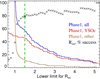 |
Fig. 8. Calibration of the Rint method through the sample and results of the adapted phase 1; see text for explanation. The vertical axis either represents the number of objects for the colored lines or percentages for the black crosses. The horizontal axis must not be interpreted as Rint values, but as Rint ranges. The finally selected criterion, Rint > 1.5, is marked in green. |
On this basis, we chose Rint > 1.5 as the optimal criterion for selecting additional YSO candidates. The green cross in Fig. 8 indicates that ∼80% of objects fulfilling the condition Rint > 1.5 are expected to be real YSOs provided that extragalactic contamination is negligible (which is justified in Appendix B.2). A plausible source of contamination is caused by nearby (< 0.6 kpc) low-mass dwarfs whose Rint would be slightly overestimated. However, only four objects fulfill Rint > 1.5 and rest < 0.6 kpc simultaneously, and all but one are too bright to be main-sequence stars. This means that red dwarfs contribute little to the overestimation of Rint.
When sources were excluded that were classified in previous sections (either as YSO candidates or as contaminants), the Rint method yielded 290 new YSO candidates, 58 (20%) of which are expected to be false positives. Of the 290 new candidates, 94 (8 of which are projected on the Cl05 region) would have never been evaluated with the classical G09 method (including its phase 2; see details in Appendix B.3).
To ensure that false-positive YSO candidates are not produced by high uncertainties, we verified that inaccurate detections were properly compensated for by averaging two or more color-color combinations. Of the 290 new candidates, only 18 Rint values are produced through a single color–color combination, and all of them are photometrically accurate enough to fulfill the uncertainty requirements for the original phase 2, except one with Rint = 6.06, which is high enough to claim that its high infrared excess is authentic.
5.1.3. Far-infrared point sources
To search for additional objects in early phases of star formation, especially those that are too deeply embedded to be detected in the mid-infrared, we examined the list of Herschel/PACS point-source detections. Within the OMEGA2000 field, 11 point sources are detected in the PACS 70 μm band, which is considered as an excellent indicator of the presence of a protostar (Dunham et al. 2008; Könyves et al. 2015). These include the source that corresponds to the Cygnus 2N massive star-forming region (already addressed in Sect. 2.5), 5 YSO candidates found through the adapted phase 1 (Sect. 5.1.1), and 1 LRP object that was discarded as a PAH-contaminated aperture (also in Sect. 5.1.1). Another 70 μm detection, whose IRAC counterpart is the brightest in the field (e.g., [5.8] = 3.93 ± 0.02), cannot be considered as an YSO because it is a carbon star according to Alksnis et al. (2001). We classify the 3 remaining sources as new candidate protostars. One of them is detected in two IRAC bands; the corresponding color (1.03 ± 0.012) is consistent with a class 0/I object.
On the other hand, 27 sources are detected only in the 160 μm band. We consider these objects as candidate starless cores based on Ragan et al. (2012), Lippok et al. (2016) (but see Feng et al. 2016).
5.2. X-ray emitting sources
During the pre-main sequence evolution, the X-ray luminosity decays much more slowly than the infrared excess (Preibisch & Feigelson 2005), which makes YSOs still detectable in X-rays even after they become indistinguishable from main-sequence stars in the infrared, that is, when they become class III sources. For this reason, X-rays are crucial for finding class III YSOs, as shown in many recent observational studies (e.g., Wang et al. 2008, 2009; Stelzer et al. 2012; Román-Zúñiga et al. 2015; Rivera-Gálvez et al. 2015). On the other hand, X-ray emission is often observed in hot luminous stars (Feigelson et al. 2007) with lifetimes of few million years (Georgy et al. 2012). Therefore X-ray point sources are ideal for pinpointing members of any young population, regardless of their evolutionary state, from YSOs to Wolf-Rayet stars.
First of all, we excluded X-ray data without reliable infrared counterparts because most of them are expected to be produced by shocks or background AGN galaxies (see Getman et al. 2005). Of the 200 likely counterparts of Chandra sources (Sect. 2.5), 7 are spectroscopic members of Berkeley 87, 1 is the foreground late-type star TYC 2684-25-1 (F8V, rest = (250 ± 1) pc), and 17 have been classified as YSO candidates in Sect. 5.1 (specifically, 10 with the adapted phase 1, and 7 with the Rint method). The 175 remaining X-ray emitters with reliable infrared counterparts are tentatively classified as class III when Rint ≤ 1.5, or as other X-ray-detected YSO candidates when Rint could not be calculated.
Still, a non-negligible amount of field stars are expected to contaminate our X-ray sample. Fortunately, the strong decay in X-ray luminosity for stars older than ≳108 yr (Micela et al. 1993; Randich 2000; Preibisch & Feigelson 2005), and for supergiants of spectral type later than B1 (Berghöfer et al. 1997; Clark et al. 2019) limits this field-star contamination to foreground stars, such as the aforementioned case of TYC 2684-25-1. This claim is supported by the Gaia distance distribution for Chandra sources (a total of 41, taking only fϖ ≤ 0.2 sources; see Sect. 4.3). This distribution is clearly bimodal: 9 objects are closer than 0.65 kpc, and all but 2 of the remaining sources are farther than 1.35 kpc away (as expected, peaking at the Berkeley 87 distance). We note that this bimodality is not observed in the cumulative histogram of Fig. 7. Consequently, we decided to remove all 10 X-ray sources that are located closer than 1 kpc from the YSO candidate list. As a result, 108 class III objects, along with 58 other YSO candidates identified through X-ray emission, were added to our list of potential members of young populations.
6. The catalog: Discussion and future work
Extinction has been estimated for 1823 (≈3.9%) of the 47 090 entries in our multiwavelength point-source catalog, distance has been calculated for 737 stars (≈1.6%) with accurate Gaia EDR3 parallaxes, and 571 sources (≈1.2%) have been classified as object types that are compatible with recent or ongoing star formation (hot stars, YSO candidates, dense cores). As a whole, at least one of these results is determined for the 3005 objects that are presented in Table 2. Further astrometric and photometric data for these sources are presented in Appendix C.
Catalog of sources with extinction, distance, or object classification results.
We consider that at least one of the properties (extinction, distance, classification) is required to potentially determine membership to one of the young populations that overlap along the line of sight. We note that proper motions are not listed because they have to be complemented with parallax information in this Galactic direction where dependence on distance is weak (see Sect. 1). This task is beyond the scope of the present work and will be presented in the next paper of this series.
Distance information (obtained directly from parallaxes or indirectly from extinction) would be desirable for every object whose classification makes it a suspected member of a young population. However, extinction or distance estimates are available only for 86 out of the 571 sources thus classified. Even worse, for the YSO candidates located within the Cl05 region (71 in total), the distance is only determined in 3 cases, being compatible with Berkeley 87 or more nearby, while extinction is estimated for another 1. This lack of extinction and distance results for the most relevant objects is caused by the following selection effects. First, YSOs are not easily detected in optical wavelengths, and specifically by Gaia, due to intrinsic reddening and extinction (especially in the case of ON2). Second, the majority of YSO candidates is intrinsically redder than Rint = 1.25, which bans them from the RJCE method (see Sect. 4.2). Third, detection in the IRAC 4.5 μm band, which is required for the RJCE method, is significantly affected by the photometric incompleteness effects described in Sect. 3.2 and Appendix B.1.
Owing to these difficulties, further analysis is required to effectively establish membership and separate the overlapping young populations, which may include not only the two clusters, but also young field stars. These objectives will be addressed in the next paper of this series, where the practical definitions established in Sect. 3.1 and the catalog published in Tables 2 and C.1 will be taken as a basis. This future work will also include other analyses that have explicitly been postponed herein, for instance, of X-ray fluxes or proper motions.
7. Conclusions
We have developed new methods for building a census of young objects in cases where distinct young populations overlap along the line of sight. In these cases, point sources are observed at a variety of distances and extinction conditions, and our flexible approach has the ability to overcome the involved selection effects.
The cornerstone of our methodology is the intrinsic reddening index, Rint, which separates intrinsically red objects from those whose color excess is caused by interstellar extinction. Unlike other previously known techniques, Rint is designed to work under conditions of significant photometric incompleteness. We have shown that in this situation, the usefulness of Rint is twofold. On the one hand, it allows avoiding intrinsically red objects when extinction estimation methods are used that are solely based on photometry (e.g., the RJCE method) because these objects would yield overestimated values. On the other hand, Rint can be used to pinpoint YSOs that would otherwise be neglected due to incomplete photometry. Based on the latter, a new method for YSO candidate selection is presented in Sect. 5.1.2.
Our methods were applied to multiwavelength observations (from the far-infrared to X-rays) of a field in which cluster formation has taken place at different distances. As a result, 571 point sources are classified as objects related to recent or ongoing star formation, with evolutionary stages ranging from starless cores to evolved hot massive stars. These include 290 YSO candidates that were found with the Rint method, ∼80% of which are expected to be real YSOs.
Table 2 lists not only objects whose classification is compatible with a young population, but also other unclassified sources whose extinction or distance estimates can lead to membership determinations. Hence, the methods and results presented here will allow distinguishing the overlapping populations and further characterizing the Berkeley 87 and [DB2001] Cl05 clusters in a forthcoming paper.
Historically, “ON2” and “Onsala 2” have been used interchangeably, either for the whole star-forming region or for its smaller constituents (H II regions, masers). This is a source of confusion for the related nomenclature because “Onsala 2N” is not related to “ON 2N”. To clarify the situation, we follow the Oskinova et al. (2010) convention in this series of papers: ON2 is the whole star-forming complex and has a size of about a quarter degree. Its northern and southern halves are called ON 2N and ON 2S, respectively. The brightest (in the mid-infrared) H II region in ON 2S, with a size of ∼2′, is G75.77+0.34. Finally, the ∼10″ sized compact H II region at the northeastern tip of G75.77+0.34 is called Cygnus 2N.
Photometric filter data were retrieved from the SVO Filter Profile Service (http://svo2.cab.inta-csic.es/svo/theory/fps).
http://irsa.ipac.caltech.edu/data/SPITZER/Cygnus-X/; see also the data delivery document at http://irsa.ipac.caltech.edu/data/SPITZER/Cygnus-X/docs/CygnusDataDelivery1.pdf
Set of Identifications, Measurements and Bibliography for Astronomical Data.
The gaiadr3_zeropoint package was downloaded from https://gitlab.com/icc-ub/public/gaiadr3_zeropoint
Acknowledgments
We thank the anonymous referee for her/his constructive comments that improved the manuscript. We are grateful to Luis Aguilar for useful suggestions about Gaia parallaxes. D.dF. acknowledges the UNAM-DGAPA postdoctoral grant, the Generalitat Valenciana APOSTD/220/228 fellowship, and the Spanish Governent AYA2015-68012-C2-2-P project. D.dF. and M.G. have received financial support from Spanish Government project ESP2017-86582-C4-1-R. C.R.-Z. acknowledges support from CONACYT project CB2017-2018 A1-S-9754. C.R.-Z. and E.J.B. acknowledge support from Programa de Apoyo a Proyectos de Investigación e Innovación Tecnológica, UNAM-DGAPA, grants IN108117 and IN109217, respectively. The scientific results reported in this article are based in part on data obtained from the Chandra Data Archive. This research has made use of software provided by the Chandra X-ray Center (CXC) in the application package CIAO. This publication makes use of data products from the Two Micron All Sky Survey, which is a joint project of the University of Massachusetts and the Infrared Processing and Analysis Center/California Institute of Technology, funded by the National Aeronautics and Space Administration and the National Science Foundation. Herschel is an ESA space observatory with science instruments provided by European-led Principal Investigator consortia and with important participation from NASA. This work has made use of data from the European Space Agency (ESA) mission Gaia (https://www.cosmos.esa.int/gaia), processed by the Gaia Data Processing and Analysis Consortium (DPAC, https://www.cosmos.esa.int/web/gaia/dpac/consortium). Funding for the DPAC has been provided by national institutions, in particular the institutions participating in the Gaia Multilateral Agreement. This research has made use of the SIMBAD database, operated at CDS, Strasbourg, France.
References
- Acke, B., & van den Ancker, M. E. 2004, A&A, 426, 151 [NASA ADS] [CrossRef] [EDP Sciences] [Google Scholar]
- Alksnis, A., Balklavs, A., Dzervitis, U., et al. 2001, Baltic Astron., 10, 1 [Google Scholar]
- Alves, J., Zucker, C., Goodman, A. A., et al. 2020, Nature, 578, 237 [NASA ADS] [CrossRef] [Google Scholar]
- Ando, K., Nagayama, T., Omodaka, T., et al. 2011, PASJ, 63, 45 [NASA ADS] [Google Scholar]
- Astraatmadja, T. L., & Bailer-Jones, C. A. L. 2016, ApJ, 832, 137 [NASA ADS] [CrossRef] [Google Scholar]
- Bailer-Jones, C. A. L. 2015, PASP, 127, 994 [NASA ADS] [CrossRef] [Google Scholar]
- Bailer-Jones, C. A. L., Rybizki, J., Fouesneau, M., Mantelet, G., & Andrae, R. 2018, AJ, 156, 58 [NASA ADS] [CrossRef] [Google Scholar]
- Barlow, M. J., & Hummer, D. G. 1982, in Wolf-Rayet Stars: Observations, Physics, Evolution, eds. C. W. H. De Loore, & A. J. Willis, IAU Symp., 99, 387 [CrossRef] [Google Scholar]
- Berghöfer, T. W., Schmitt, J. H. M. M., Danner, R., & Cassinelli, J. P. 1997, A&A, 322, 167 [Google Scholar]
- Berlanas, S. R., Wright, N. J., Herrero, A., Drew, J. E., & Lennon, D. J. 2019, MNRAS, 484, 1838 [NASA ADS] [Google Scholar]
- Bertin, E., & Arnouts, S. 1996, A&AS, 117, 393 [NASA ADS] [CrossRef] [EDP Sciences] [Google Scholar]
- Bessell, M. S., & Brett, J. M. 1988, PASP, 100, 1134 [NASA ADS] [CrossRef] [Google Scholar]
- Bhavya, B., Mathew, B., & Subramaniam, A. 2007, Bull. Astron. Soc. India, 35, 383 [Google Scholar]
- Binder, B. A., & Povich, M. S. 2018, ApJ, 864, 136 [NASA ADS] [CrossRef] [Google Scholar]
- Cantat-Gaudin, T., Jordi, C., Vallenari, A., et al. 2018, A&A, 618, A93 [NASA ADS] [CrossRef] [EDP Sciences] [Google Scholar]
- Capitanio, L., Lallement, R., Vergely, J. L., Elyajouri, M., & Monreal-Ibero, A. 2017, A&A, 606, A65 [NASA ADS] [CrossRef] [EDP Sciences] [Google Scholar]
- Carpenter, J. M. 2001, AJ, 121, 2851 [NASA ADS] [CrossRef] [Google Scholar]
- Chen, P. S., Shan, H. G., & Zhang, P. 2016, New Astron., 44, 1 [NASA ADS] [CrossRef] [Google Scholar]
- Cho, S.-H., Yun, Y., Kim, J., et al. 2016, ApJ, 826, 157 [Google Scholar]
- Clark, J. S., Ritchie, B. W., & Negueruela, I. 2019, A&A, 626, A59 [NASA ADS] [CrossRef] [EDP Sciences] [Google Scholar]
- Cohen, M., Barlow, M. J., & Kuhi, L. V. 1975, A&A, 40, 291 [NASA ADS] [Google Scholar]
- Comerón, F., & Torra, J. 2001, A&A, 375, 539 [NASA ADS] [CrossRef] [EDP Sciences] [Google Scholar]
- Dias, W. S., Monteiro, H., Caetano, T. C., et al. 2014, A&A, 564, A79 [NASA ADS] [CrossRef] [EDP Sciences] [Google Scholar]
- Dotter, A., Chaboyer, B., Jevremović, D., et al. 2008, ApJS, 178, 89 [Google Scholar]
- Drew, J. E., Barlow, M. J., Unruh, Y. C., et al. 2004, MNRAS, 351, 206 [NASA ADS] [CrossRef] [Google Scholar]
- Ducati, J. R., Bevilacqua, C. M., Rembold, S. B., & Ribeiro, D. 2001, ApJ, 558, 309 [NASA ADS] [CrossRef] [Google Scholar]
- Dunham, M. M., Crapsi, A., Evans, N. J., II, et al. 2008, ApJS, 179, 249 [NASA ADS] [CrossRef] [Google Scholar]
- Dutra, C. M., & Bica, E. 2001, A&A, 376, 434 [NASA ADS] [CrossRef] [EDP Sciences] [Google Scholar]
- Ellsworth-Bowers, T. P., Rosolowsky, E., Glenn, J., et al. 2015, ApJ, 799, 29 [Google Scholar]
- Feigelson, E., Townsley, L., Güdel, M., & Stassun, K. 2007, Protostars and Planets V, 313 [Google Scholar]
- Feng, S., Beuther, H., Zhang, Q., et al. 2016, ApJ, 828, 100 [NASA ADS] [CrossRef] [Google Scholar]
- Freeman, P. E., Kashyap, V., Rosner, R., & Lamb, D. Q. 2002, ApJS, 138, 185 [Google Scholar]
- Fruscione, A., McDowell, J. C., Allen, G. E., et al. 2006, in Proc. SPIE, 6270, 62701V [Google Scholar]
- Furlan, E., Hartmann, L., Calvet, N., et al. 2006, ApJS, 165, 568 [NASA ADS] [CrossRef] [MathSciNet] [Google Scholar]
- Gaia Collaboration (Prusti, T., et al.) 2016, A&A, 595, A1 [NASA ADS] [CrossRef] [EDP Sciences] [Google Scholar]
- Gaia Collaboration (Brown, A. G. A., et al.) 2021, A&A, 649, A1 [NASA ADS] [CrossRef] [EDP Sciences] [Google Scholar]
- Gehrz, R. D., Hackwell, J. A., & Jones, T. W. 1974, ApJ, 191, 675 [NASA ADS] [CrossRef] [Google Scholar]
- Georgy, C., Ekström, S., Meynet, G., et al. 2012, A&A, 542, A29 [NASA ADS] [CrossRef] [EDP Sciences] [Google Scholar]
- Getman, K. V., Feigelson, E. D., Grosso, N., et al. 2005, ApJS, 160, 353 [Google Scholar]
- Giovannelli, F. 2002, Mem. Soc. Astron. It., 73, 920 [Google Scholar]
- Griffin, M. J., Abergel, A., Abreu, A., et al. 2010, A&A, 518, L3 [EDP Sciences] [Google Scholar]
- Gutermuth, R. A., Myers, P. C., Megeath, S. T., et al. 2008, ApJ, 674, 336 [NASA ADS] [CrossRef] [Google Scholar]
- Gutermuth, R. A., Megeath, S. T., Myers, P. C., et al. 2009, ApJS, 184, 18 [NASA ADS] [CrossRef] [Google Scholar]
- Harris, S. 1974, MNRAS, 166, 29 [CrossRef] [Google Scholar]
- Hernández, J., Hartmann, L., Megeath, T., et al. 2007, ApJ, 662, 1067 [NASA ADS] [CrossRef] [Google Scholar]
- Hewett, P. C., Warren, S. J., Leggett, S. K., & Hodgkin, S. T. 2006, MNRAS, 367, 454 [NASA ADS] [CrossRef] [Google Scholar]
- Hodgkin, S. T., Irwin, M. J., Hewett, P. C., & Warren, S. J. 2009, MNRAS, 394, 675 [NASA ADS] [CrossRef] [Google Scholar]
- Indebetouw, R., Mathis, J. S., Babler, B. L., et al. 2005, ApJ, 619, 931 [NASA ADS] [CrossRef] [Google Scholar]
- Könyves, V., André, P., Men’shchikov, A., et al. 2015, A&A, 584, A91 [NASA ADS] [CrossRef] [EDP Sciences] [Google Scholar]
- Lada, C. J., Muench, A. A., Luhman, K. L., et al. 2006, AJ, 131, 1574 [Google Scholar]
- Lallement, R., Capitanio, L., Ruiz-Dern, L., et al. 2018, A&A, 616, A132 [NASA ADS] [CrossRef] [EDP Sciences] [Google Scholar]
- Lawrence, A., Warren, S. J., Almaini, O., et al. 2007, MNRAS, 379, 1599 [NASA ADS] [CrossRef] [MathSciNet] [Google Scholar]
- Le Duigou, J. M., & Knödlseder, J. 2002, A&A, 392, 869 [NASA ADS] [CrossRef] [EDP Sciences] [Google Scholar]
- Levine, J. L. 2006, PhD Thesis, University of Florida, USA [Google Scholar]
- Lim, B., Nazé, Y., Gosset, E., & Rauw, G. 2019, MNRAS, 490, 440 [NASA ADS] [CrossRef] [Google Scholar]
- Lindegren, L., Bastian, U., Biermann, M., et al. 2021, A&A, 649, A4 [EDP Sciences] [Google Scholar]
- Lippok, N., Launhardt, R., Henning, T., et al. 2016, A&A, 592, A61 [NASA ADS] [CrossRef] [EDP Sciences] [Google Scholar]
- Luri, X., Brown, A. G. A., Sarro, L. M., et al. 2018, A&A, 616, A9 [NASA ADS] [CrossRef] [EDP Sciences] [Google Scholar]
- Majaess, D. J., Turner, D. G., Lane, D. J., & Moncrieff, K. E. 2008, J. Am. Assoc. Variable Star Observers, 36, 90 [Google Scholar]
- Majewski, S. R., Zasowski, G., & Nidever, D. L. 2011, ApJ, 739, 25 [NASA ADS] [CrossRef] [MathSciNet] [Google Scholar]
- Martins, F., & Plez, B. 2006, A&A, 457, 637 [NASA ADS] [CrossRef] [EDP Sciences] [Google Scholar]
- Marton, G., Calzoletti, L., Perez Garcia, A. M., et al. 2017, ArXiv e-prints [arXiv:1705.05693] [Google Scholar]
- Massey, P., DeGioia-Eastwood, K., & Waterhouse, E. 2001, AJ, 121, 1050 [NASA ADS] [CrossRef] [Google Scholar]
- Mathew, B., Banerjee, D. P. K., Subramaniam, A., & Ashok, N. M. 2012, ApJ, 753, 13 [NASA ADS] [CrossRef] [Google Scholar]
- Matthews, H. E., Goss, W. M., Winnberg, A., & Habing, H. J. 1973, A&A, 29, 309 [NASA ADS] [Google Scholar]
- Mauerhan, J. C., Van Dyk, S. D., & Morris, P. W. 2011, AJ, 142, 40 [NASA ADS] [CrossRef] [Google Scholar]
- Micela, G., Sciortino, S., & Favata, F. 1993, ApJ, 412, 618 [NASA ADS] [CrossRef] [Google Scholar]
- Moscadelli, L., Sanna, A., Goddi, C., et al. 2019, A&A, 631, A74 [NASA ADS] [CrossRef] [EDP Sciences] [Google Scholar]
- Negueruela, I. 2004, Astron. Nachr., 325, 380 [Google Scholar]
- Oskinova, L. M., Hamann, W. R., Feldmeier, A., Ignace, R., & Chu, Y. H. 2009, ApJ, 693, L44 [NASA ADS] [CrossRef] [Google Scholar]
- Oskinova, L. M., Gruendl, R. A., Ignace, R., et al. 2010, ApJ, 712, 763 [CrossRef] [Google Scholar]
- Pilbratt, G. L., Riedinger, J. R., Passvogel, T., et al. 2010, A&A, 518, L1 [CrossRef] [EDP Sciences] [Google Scholar]
- Pipenbrink, A., & Wendker, H. J. 1988, A&A, 191, 313 [Google Scholar]
- Poglitsch, A., Waelkens, C., Geis, N., et al. 2010, A&A, 518, L2 [NASA ADS] [CrossRef] [EDP Sciences] [Google Scholar]
- Polcaro, V. F., & Norci, L. 1998, A&A, 339, 75 [NASA ADS] [Google Scholar]
- Polcaro, V. F., Rossi, C., Norci, L., & Giovannelli, F. 1989, Acta Astron., 39, 323 [Google Scholar]
- Polcaro, V. F., Rossi, C., Persi, P., et al. 1991, Mem. Soc. Astron. It., 62, 933 [Google Scholar]
- Preibisch, T., & Feigelson, E. D. 2005, ApJS, 160, 390 [Google Scholar]
- Ragan, S., Henning, T., Krause, O., et al. 2012, A&A, 547, A49 [NASA ADS] [CrossRef] [EDP Sciences] [Google Scholar]
- Randich, S. 2000, in Stellar Clusters and Associations: Convection, Rotation, and Dynamos, eds. R. Pallavicini, G. Micela, & S. Sciortino, ASP Conf. Ser., 198, 401 [Google Scholar]
- Rate, G., Crowther, P. A., & Parker, R. J. 2020, MNRAS, 495, 1209 [CrossRef] [Google Scholar]
- Reipurth, B., & Schneider, N. 2008, Star Formation and Young Clusters in Cygnus (ASP Monograph Publications), 4, 36 [Google Scholar]
- Rieke, G. H., & Lebofsky, M. J. 1985, ApJ, 288, 618 [Google Scholar]
- Rivera-Gálvez, S., Román-Zúñiga, C. G., Jiménez-Bailón, E., et al. 2015, AJ, 150, 191 [NASA ADS] [CrossRef] [Google Scholar]
- Román-Zúñiga, C. G. 2006, PhD Thesis, University of Florida, USA [Google Scholar]
- Román-Zúñiga, C. G., Ybarra, J. E., Megías, G. D., et al. 2015, AJ, 150, 80 [NASA ADS] [CrossRef] [Google Scholar]
- Rots, A. H., & Budavári, T. 2011, ApJS, 192, 8 [NASA ADS] [CrossRef] [Google Scholar]
- Rygl, K. L. J., Brunthaler, A., Sanna, A., et al. 2012, A&A, 539, A79 [NASA ADS] [CrossRef] [EDP Sciences] [Google Scholar]
- Sánchez-Monge, Á., Kurtz, S., Palau, A., et al. 2013, ApJ, 766, 114 [Google Scholar]
- Sander, A. A. C., Hamann, W. R., Todt, H., et al. 2019, A&A, 621, A92 [NASA ADS] [CrossRef] [EDP Sciences] [Google Scholar]
- Schneider, N., Bontemps, S., Simon, R., et al. 2006, A&A, 458, 855 [NASA ADS] [CrossRef] [EDP Sciences] [Google Scholar]
- Skinner, S. L., Sokal, K. R., & Güdel, M. 2019, ApJ, 871, 116 [CrossRef] [Google Scholar]
- Skrutskie, M. F., Cutri, R. M., Stiening, R., et al. 2006, AJ, 131, 1163 [NASA ADS] [CrossRef] [Google Scholar]
- Sokal, K. R., Skinner, S. L., Zhekov, S. A., Güdel, M., & Schmutz, W. 2010, ApJ, 715, 1327 [NASA ADS] [CrossRef] [Google Scholar]
- Stelzer, B., Preibisch, T., Alexander, F., et al. 2012, A&A, 537, A135 [NASA ADS] [CrossRef] [EDP Sciences] [Google Scholar]
- Taylor, M. B. 2005, in Astronomical Data Analysis Software and Systems XIV, eds. P. Shopbell, M. Britton, & R. Ebert, ASP Conf. Ser., 347, 29 [Google Scholar]
- Teixeira, P. S., Lada, C. J., Marengo, M., & Lada, E. A. 2012, A&A, 540, A83 [NASA ADS] [CrossRef] [EDP Sciences] [Google Scholar]
- Townsley, L. K., Broos, P. S., Garmire, G. P., et al. 2014, ApJS, 213, 1 [NASA ADS] [CrossRef] [Google Scholar]
- Townsley, L. K., Broos, P. S., Garmire, G. P., et al. 2018, ApJS, 235, 43 [NASA ADS] [CrossRef] [Google Scholar]
- Townsley, L. K., Broos, P. S., Garmire, G. P., & Povich, M. S. 2019, ApJS, 244, 28 [CrossRef] [Google Scholar]
- Tramper, F., Straal, S. M., Sanyal, D., et al. 2015, A&A, 581, A110 [NASA ADS] [CrossRef] [EDP Sciences] [Google Scholar]
- Turner, D. G., & Forbes, D. 1982, PASP, 94, 789 [NASA ADS] [CrossRef] [Google Scholar]
- Turner, D. G., Rohanizadegan, M., Berdnikov, L. N., & Pastukhova, E. N. 2006, PASP, 118, 1533 [NASA ADS] [CrossRef] [Google Scholar]
- Uyanıker, B., Fürst, E., Reich, W., Aschenbach, B., & Wielebinski, R. 2001, A&A, 371, 675 [NASA ADS] [CrossRef] [EDP Sciences] [Google Scholar]
- Voroshilov, V. I., Kolesnik, L. N., & Kuznetsov, V. I. 1976, Catalogue of BV Magnitudes and Spectral Classes of 18000 Stars [Google Scholar]
- Wang, J., Townsley, L. K., Feigelson, E. D., et al. 2008, ApJ, 675, 464 [NASA ADS] [CrossRef] [Google Scholar]
- Wang, J., Feigelson, E. D., Townsley, L. K., et al. 2009, ApJ, 696, 47 [NASA ADS] [CrossRef] [Google Scholar]
- Wenger, M., Ochsenbein, F., Egret, D., et al. 2000, A&AS, 143, 9 [NASA ADS] [CrossRef] [EDP Sciences] [Google Scholar]
- Xu, Y., Li, J. J., Reid, M. J., et al. 2013, ApJ, 769, 15 [NASA ADS] [CrossRef] [Google Scholar]
- Zucker, C., Speagle, J. S., Schlafly, E. F., et al. 2019, ApJ, 879, 125 [NASA ADS] [CrossRef] [Google Scholar]
- Zucker, C., Speagle, J. S., Schlafly, E. F., et al. 2020, A&A, 633, A51 [CrossRef] [EDP Sciences] [Google Scholar]
Appendix A: Details on the intrinsic reddening index
As introduced in Sect. 3.2, Rint is defined in terms of the position of the sources in color–color diagrams whose horizontal and vertical axes area mid-infrared color X = X2 − X1 and a near-infrared color Y = Y2 − Y1, respectively. We avoided colors that include the longest IRAC wavelegths ([5.8] and [8.0]) because the small number of detections in these bands would make them impractical for a relatively homogeneous study of the whole stellar population. Regarding the near-infrared colors, J − H is in principle best suited to isolating interstellar reddening, as in Teixeira et al. (2012). However, because J is missing in a large fraction (≈14%) of sources detected in H and K we included H − K as well. Therefore the following options for X and Y are allowed: X = K − [3.6], X = K − [4.5], X = [3.6]−[4.5]; and Y = J − H, Y = H − K.
In the six resulting color–color diagrams (Fig. A.1), the extinction vector is drawn according to the Indebetouw et al. (2005) law. Because the AK value provided by these authors refers to the 2MASS KS band, we applied the correction AK/AKS = 0.98, which we obtained through approximate interpolation of the Indebetouw et al. (2005) law at the effective wavelength of the UKIDSS K bandpass.
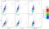 |
Fig. A.1. Color–color diagrams that are used to compute Rint, which is coded as indicated in the color bars for LRP and HRP sources. The reddening band boundaries that are used as a reference (see text) are drawn as dashed pink lines. The 1 Gyr isochrone for solar abundances is drawn in black. The average photometric errors are shown as brown bars just below the β values. |
The next step is to determine in each diagram the boundary between the interstellar reddening band of normal stars and the region in which intrinsically red stars should be placed. More specifically, the boundary at which for each given Y value, X becomes too red to be consistent with a normal star that is only affected by interstellar extinction. To represent a typical population of unreddened stars (such as those found throughout the Galactic disk outside star-forming regions), a 1 Gyr isochrone for solar abundances was taken from the Dartmouth Stellar Evolution Database (Dotter et al. 2008). In each diagram, normal stars are expected to lie within the reddening band that results from sliding the isochrone (shown as a black curve) along the direction of the extinction vector. The limit of the reddening band with the reddest X values (although not strictly, as we clarify below) is the boundary we are looking for. In each Fig. A.1 diagram, the boundary (dashed pink line) follows the equation
 (A.1)
(A.1)
and β(X, Y) takes the value that is printed in the corresponding panel of Fig. A.1. A strict compliance with this boundary definition would imply that all the isochrone data points would have bluer X colors than the boundary. In some cases, however, the sole contribution of low-mass objects, which are not expected to be detectable at Cygnus-X distances, pushes the boundary toward significantly redder colors. To avoid this undesirable effect, the low-mass end of the isochrone was ignored in these cases, and any possible contamination in the foreground (where low-mass stars are detectable) is assessed in Sect. 5.1.2.
Then, for each diagram (X, Y), the relative shift from the reddening band boundary is defined as
![Mathematical equation: $$ \begin{aligned} S_{X,Y} = \frac{X-\left[Y-\beta (X,Y)\right]/\alpha (X,Y)}{\log (\lambda _{X_2} / \lambda _{X_1})} \,, \end{aligned} $$](/articles/aa/full_html/2021/06/aa40065-20/aa40065-20-eq30.gif) (A.2)
(A.2)
and λ stands for the effective wavelength of the corresponding filter. We remark that the shift is defined as relative to the corresponding color baseline, Δ log λ.
Finally, Rint is computed as a weighted average of relative shifts as expressed in Eq. (1). This Rint definition implies that a hypothetical data point that is simultaneously located at all the reddening band boundaries would yield Rint = 1. The weights in Eq. (1) can be tailored to the scientific goals that are addressed; in this work, we chose the following weights that depend on the relative photometric uncertainties:
 (A.3)
(A.3)
Appendix B: Description and treatment of relevant selection biases
B.1. Purely photometric biases affecting the G09 method
Phase 1 of the G09 method requires that sources are simultaneously detected in all four IRAC bands with photometric uncertainties lower than 0.2, while only the [5.8] and [8.0] bands can be waived for phase 2 (which in return needs at least H and K with σ < 0.1). We remark that these conditions are required for being merely evaluated by the method before any classification criteria are applied. Our data are affected by these restrictions in the following ways. First, they would confine our YSO search to the portion of the OMEGA2000 field that is covered by all the four IRAC bands (hereafter the NIR+MIR region; see also Fig. 1), spanning roughly 158 arcmin2. Second, the density of detections meeting the phase 1 requirements decreases toward the Cl05 region (as defined in Sect. 3.1) despite the near-infrared overdensity. The latter is better illustrated in Fig. B.1, which shows the number and distribution of photometric detections in each band for the Cl05 region relative to the NIR+MIR region.
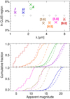 |
Fig. B.1. Illustration of selection biases affecting infrared photometry in the Cl05 region relative to the NIR+MIR region. Top: proportion of detections falling within the Cl05 region, as computed by considering all detections (squares), or only those meeting the corresponding uncertainty requirement for the G09 method (crosses). For comparison, the case of a spatially uniform distribution is shown as gray diamonds. Bottom: cumulative histograms of apparent magnitudes in the Cl05 region (solid lines) and the whole NIR+MIR region (dashed), using the same uncertainty-limited sample as for the crosses in the top panel and the same color code. |
The top panel of Fig. B.1 reveals that the overdensity of near-infrared sources in the Cl05 region, which is especially conspicuous in the K band, turns into an underdensity in IRAC wavelengths, where YSOs were supposed to appear highlighted. This problem is caused by the combined effects of large distance toward ON2 (relative to the regions studied by Gutermuth et al. 2008, 2009) and the IRAC technical features. On the one hand, stellar crowding in [DB2001] Cl05 appears to be excessive for the limited spatial resolution of IRAC (compared to OMEGA2000), which leads to strong source confusion effects. On the other hand, the presence of distant bright clouds aligned with point sources makes the latter hard to detect due to low contrast between both components, which significantly worsens with the distance to the observer. While the measured flux of a point source decreases as 1/r2, the surface brightness of the cloud remains constant (because the covered solid angle also decreases as 1/r2). This effect is particularly strong in the bands that are more affected by PAH emission, [5.8] and [8.0].
Still, a slight increase toward the longest wavelengths is noticeable in the top panel of Fig. B.1, which is interpreted as the presence of disks that slightly compensate for the selection bias.
These biases are not only detrimental to source counts, but also to the magnitude ranges in which the G09 method can be used, as shown in the lower plots of Fig. B.1. Cumulative histograms therein reveal that the G09 method is biased against faint objects in the Cl05 region in comparison with the NIR+MIR field. Although this occurs in every photometric band, the differences between the two samples are larger for the IRAC photometry, and especially in the [5.8] and [8.0] bands, where only detections in the bright tail of the distribution survive contamination from extended PAH emission.
Altogether, the original G09 method can be applied to 3718 sources, 58 (1.56%) of which are part of the Cl05 region. When we only focus on phase 1, 480 sources in total can be assessed, 10 of which (2.1%) lie inside the Cl05 circle. Despite the overdensity of red objects, these proportions are notably lower than the corresponding ratio of solid angles, 3.1%, that would match a spatially uniform distribution. A strict application of the G09 method would indeed miss a very significant part of red sources just in the region where YSOs are expected to be concentrated.
B.2. Extinction-related biases
To distinguish YSO candidates from extragalactic contaminants, the original G09 method included constraints in [4.5] (namely, [4.5]PAH > 11.5; [4.5]BL-AGN > 13.5) that were based on the apparent magnitude distribution of YSOs in the nearest kiloparsec (Gutermuth et al. 2008). In the ON2 region, however, we expect to find YSOs at about four times that distance, implying a brightness decrease of ∼3 mag. Another half magnitude should be added to [4.5] because of the additional foreground extinction (ΔAV ∼ 10, converted through Rieke & Lebofsky 1985; Indebetouw et al. 2005) relative to the Gutermuth et al. (2009) sample. As a consequence, the G09 method would erroneously have discarded any YSOs that fall within a 3.5 mag range from the original limits (i.e., 11.5 < [4.5]PAH < 15; 13.5 < [4.5]BL-AGN < 17).
This issue cannot be simply solved by shifting the [4.5] boundaries accordingly because galaxies might still be present as contaminators within that 3.5 mag range. Extragalactic light is attenuated by interstellar extinction while traveling throughout the Galactic disk, starting from some point far beyond ON2. The total extinction must be higher than the most extinguished stellar populations observed in off-cloud regions, that is, a few dozen visual magnitudes (based on the extent of color–color diagrams along the extinction vector, see, e.g., Fig. 6b). Taking a conservative approach, we assume ΔA[4.5] = 1 (roughly equivalent to ΔAV ≈ 20) for extragalactic sources (relative to the negligible extinction of the Bootes field used by Gutermuth et al. 2008). In our field, the five sources initially categorized as BL-AGN candidates are in the range 13.5 < [4.5] < 14.5, therefore this one-magnitude dimming is enough to simply skip the step of finding BL-AGN contaminants.
The case of extragalactic PAH candidates is more complicated because only 3 out of the 14 initially selected sources lie in the range 11.5 < [4.5] < 12.5. To assess the degree of contamination by PAH galaxies still present among the 11 remaining objects, we relied on the power law that Gutermuth et al. (2008) fit to the differential surface density of PAH galaxies (σPAH([5.8])) in the Bootes field. When we assume a representative color [4.5]−[5.8]≈0.5 for PAH galaxies based on Gutermuth et al. (2009, Fig. 13) and take into account the additional extinction for the ON2 direction relative to Bootes,
![Mathematical equation: $$ \begin{aligned} \sigma _\mathrm{PAH} ^\mathrm{(ON2)} (12.5<[4.5]<15) \approx \sigma _\mathrm{PAH} ^\mathrm{(Boo)} (11 < [5.8] < 13.5) \nonumber \\ = 2 \int _{11}^{13.5} 10^{-18.24} [5.8]^{17.02}\ \mathrm{d} [5.8] = 14.6\,\mathrm{deg} ^{-2}, \end{aligned} $$](/articles/aa/full_html/2021/06/aa40065-20/aa40065-20-eq32.gif) (B.1)
(B.1)
where the factor 2 takes into account that σPAH([5.8]) is defined per half-magnitude bin (Gutermuth et al. 2008). Equation (B.1) implies that the expected number of PAH galaxies within the solid angle covered by the NIR+MIR field is 0.64, or equivalently, that the 11 sources described above have a ∼7% probability each of being a PAH galaxy. If we allow some likelihood of 1 or 2 PAH galaxies that are still misidentified as YSOs, we can therefore skip the elimination of PAH galaxies as we did for BL-AGN candidates above.
Finally, we have to ensure that the Rint method (Sect. 5.1.2) is not affected by extragalactic contaminants. The H-band magnitude that is required by the method is more affected by extinction than mid-infrared bands. Specifically, our above established assumption of ΔA[4.5] = 1 for extragalactic sources would be converted into ΔAH ≈ 3.6 (through Indebetouw et al. 2005). This high H-band extinction is sufficient to cause the relevant extragalactic contaminants to become unobservable (i.e., those that are faint enough not to be detectable in [8.0] or [5.8] despite their YSO-like colors).
B.3. Benefits of Rint for the sample that can be assessed
In this section, we provide a detailed comparison between the point-source samples that can be evaluated by the Rint method (Sect. 5.1.2) and phase 2 of the G09 method. First, we note that all sources that can be assessed with the G09 method can also be evaluated with our whole method (which consists of the adapted phase 1 plus the Rint method), but not vice versa.
Overall, our whole method is capable of evaluating 5048 sources in the OMEGA2000 field, a ∼36% gain relative to the 3718 from Appendix B.1. This increase is in great part attributable to 915 Rint objects in the region that lack 4.5 μm observations; therefore the gain is reduced to only 11% when the remaining solid angle is considered (i.e., in the NIR+MIR region). The superiority of the Rint method is stronger in the Cl05 region, where 75 objects are evaluated, a ∼29% gain (cf. 58 objects from Appendix B.1). Hence it is clear that the Rint method helps mitigate the effects of the selection bias addressed in Appendix B.1 to a significant extent.
When we only focus on the new 290 YSO candidates with Rint > 1.5, the usefulness of the method is even clearer. At least 94 of these would never have been evaluated with the G09 method owing to missing or inaccurate detection in some photometric band. Within the Cl05 region, the G09 method would be unable to assess 8 out of 34 new YSO candidates.
Appendix C: Astrometric and photometric data
Table C.1 shows the astrometric and infrared photometric data for all sources listed in Table 2. We only present astrometric information for the X-ray sources that is relevant to counterpart matching, while X-ray fluxes are postponed to the next paper of this series.
Astrometric data and infrared photometry for the sources listed in Table 2.
All Tables
All Figures
|
Fig. 1. Left: spatial coverage of the OMEGA2000, Chandra, and IRAC observations in the 3.6 μm image of the ON2 region. Right: RGB image (R = [8.0],G = [4.5],B = [3.6]) of the region that is covered by coordinate axes in the left panel, and showing the OMEGA2000 field of view in the same way. Green circles show the position and size of Berkeley 87 (dashed) and [DB2001] Cl05 according to Dias et al. (2014) and Dutra & Bica (2001), respectively. The Cygnus 2N region is marked as a yellow diamond. |
| In the text | |
|
Fig. 2. Photometric calibration of OMEGA2000 (“O2”) data. Panel a: comparison of calibration diagrams using 2MASS or UKIDSS as the reference (“ref”) survey. Panel b: location of J-band point sources (colored crosses: JUKIDSS < 17; σJ < 0.035) relative to the flat-field artifact, see Sect. 2.1. Panel c: close-up view of panel a showing the J-band bimodality; symbols are as in panel b. |
| In the text | |
|
Fig. 3. Comparison of X-ray detection ellipses in three 40″ × 40″ closeups, centered at the coordinates that are printed in blue, of the 2009 (left) and 2016 (right) Chandra/ACIS fields, using binning factors of 1 (green), 2 (yellow), and 4 (purple) pixels. Ellipses that were selected for the final source list are drawn with solid lines. The background images are 2-pixel binned. Upper panels: portion of the [DB2001] Cl05 cluster, middle panels: region near the edge of the 2016 field, and lower panels: region near the 2009 edge. |
| In the text | |
|
Fig. 4. Histogram of angular separations between X-ray and infrared point sources (after absolute astrometric calibration with Gaia). Gray bars include all coincidences, and the blue line only accounts for the nearest infrared neighbor of each X-ray source. Green bars are the number of infrared sources that were finally accepted as counterparts, and the orange portions were marked as doubtful. As a reference, black crosses show the case of a random source distribution (indicative of a case in which all coincidences are spurious). |
| In the text | |
|
Fig. 5. OMEGA2000 K-band image (grayscale) and point-source catalog (small blue crosses) of the Cygnus 2N region. The Herschel/PACS 70 μm map is overplotted as contours with an interval of 3.5 Jy arcsec−2; the positions of the 70 μm and 160 μm detections according to the Herschel public catalog are marked as orange and red circles, respectively. Chandra detection ellipses are drawn as dashed blue lines, and infrared sources detected by Spitzer at wavelengths larger than 5 μm are shown as large pink crosses. The remaining symbols indicate objects reported by Sánchez-Monge et al. (2013): green and turquoise pluses are methanol and water masers, respectively, and purple squares are the centimeter continuum sources that were called CORE (C), EAST (E), and UCHII (U) by these authors. |
| In the text | |
|
Fig. 6. Multiwavelength RGB images (colored as indicated in the upper left corner of each image) of the Berkeley 87/ON2 region, and infrared color–color diagram of the OMEGA2000 field. The extinction vector that is shown in this diagram (panel b) is obtained from Indebetouw et al. (2005), and taking AK/AKS ≈ 0.98 (which is justified in Appendix A). In all the images, the Cl05 region is enclosed by a white or black circle. In the Herschel RGB image (d), the OMEGA2000 field coverage is shown as a white square. An infrared closeup of this field, centered on [DB2001] Cl05, is displayed in panel a, and its Chandra counterpart is shown in panel c. The latter is made of 2-pixel binned images from the 2009 observation; the density of J − H > 1.7 sources is drawn as gray contours (dotted = 55 arcmin−2; dashed = 110 arcmin−2). In all panels, Berkeley 87 spectroscopic members are marked as open blue diamonds, except for WR 142, which is shown as an open blue circle (only in panels b and d); crosses are point sources within the Cl05 region that are simultaneously detected in J, H, K, and [5.8] (i.e., those that are represented in panel b). |
| In the text | |
|
Fig. 7. Visual extinction vs. distance estimates, colored as follows: blue shows spectroscopically confirmed Berkeley 87 members, orange shows photometric candidates for Berkeley 87 membership according to Turner & Forbes (1982), magenta shows additional stars of known spectral types, black shows sources that were not previously cataloged, and gray is explained below. Objects whose AV values are obtained in Sects. 4.1 and 4.2 are shown as crosses and diamonds, respectively. The Berkeley 87 distance and AV range are represented as a green rectangle. The extinction along the Berkeley 87 direction according to the Stilism map is drawn as a solid black curve. The errors are shown as dotted lines. The dashed red curve is the cumulative distribution (see the scale on the right axis) for the sample of 737 objects with valid distance results, i.e., those that fulfill 0 < fϖ ≤ 0.2. The gray data point is not part of this sample and is only included to illustrate the effects of relaxing the fϖ constraints (see text). |
| In the text | |
|
Fig. 8. Calibration of the Rint method through the sample and results of the adapted phase 1; see text for explanation. The vertical axis either represents the number of objects for the colored lines or percentages for the black crosses. The horizontal axis must not be interpreted as Rint values, but as Rint ranges. The finally selected criterion, Rint > 1.5, is marked in green. |
| In the text | |
|
Fig. A.1. Color–color diagrams that are used to compute Rint, which is coded as indicated in the color bars for LRP and HRP sources. The reddening band boundaries that are used as a reference (see text) are drawn as dashed pink lines. The 1 Gyr isochrone for solar abundances is drawn in black. The average photometric errors are shown as brown bars just below the β values. |
| In the text | |
|
Fig. B.1. Illustration of selection biases affecting infrared photometry in the Cl05 region relative to the NIR+MIR region. Top: proportion of detections falling within the Cl05 region, as computed by considering all detections (squares), or only those meeting the corresponding uncertainty requirement for the G09 method (crosses). For comparison, the case of a spatially uniform distribution is shown as gray diamonds. Bottom: cumulative histograms of apparent magnitudes in the Cl05 region (solid lines) and the whole NIR+MIR region (dashed), using the same uncertainty-limited sample as for the crosses in the top panel and the same color code. |
| In the text | |
Current usage metrics show cumulative count of Article Views (full-text article views including HTML views, PDF and ePub downloads, according to the available data) and Abstracts Views on Vision4Press platform.
Data correspond to usage on the plateform after 2015. The current usage metrics is available 48-96 hours after online publication and is updated daily on week days.
Initial download of the metrics may take a while.