| Issue |
A&A
Volume 650, June 2021
|
|
|---|---|---|
| Article Number | A48 | |
| Number of page(s) | 17 | |
| Section | Galactic structure, stellar clusters and populations | |
| DOI | https://doi.org/10.1051/0004-6361/202039899 | |
| Published online | 04 June 2021 | |
New low-mass members of Chamaeleon I and ϵ Cha
1
CENTRA, Faculdade de Ciências, Universidade de Lisboa, Ed. C8, Campo Grande, 1749-016 Lisboa, Portugal
e-mail: This email address is being protected from spambots. You need JavaScript enabled to view it.
2
School of Physics & Astronomy, University of St Andrews, North Haugh, St Andrews KY169SS, UK
Received:
12
November
2020
Accepted:
7
February
2021
Abstract
Aims. The goal of this paper is to increase the membership list of the Chamaeleon star-forming region and the ϵ Cha moving group, in particular for low-mass stars and substellar objects. We extended the search region significantly beyond the dark clouds.
Methods. Our sample has been selected based on proper motions and colours obtained from Gaia and 2MASS. We present and discuss the optical spectroscopic follow-up of 18 low-mass stellar objects in Cha I and ϵ Cha. We characterize the properties of objects by deriving their physical parameters from spectroscopy and photometry.
Results. We add three more low-mass members to the list of Cha I and increase the census of known ϵ Cha members by more than 40%, thereby spectroscopically confirming 13 new members and relying on X-ray emission as youth indicator for 2 more. In most cases the best-fitting spectral template is from objects in the TW Hya association, indicating that ϵ Cha has a similar age. The first estimate of the slope of the initial mass function in ϵ Cha down to the substellar regime is consistent with that of other young clusters. We estimate our initial mass function (IMF) to be complete down to ≈0.03 M⊙. The IMF can be represented by two power laws: for M < 0.5 M⊙ α = 0.42 ± 0.11 and for M > 0.5 M⊙ α = 1.44 ± 0.12.
Conclusions. We find similarities between ϵ Cha and the southernmost part of Lower Centaurus Crux (LCC A0), which lie at similar distances and share the same proper motions. This suggests that ϵ Cha and LCC A0 may have been born during the same star formation event
Key words: stars: low-mass / stars: pre-main sequence / open clusters and associations: individual: ϵ Cha young moving group / brown dwarfs
© ESO 2021
1. Introduction
The Chamaeleon molecular cloud complex is one of the nearest sites of star formation and dominates the dust extinction maps of the region (Luhman et al. 2008). The complex and its surroundings are abundant with pre-main-sequence stars of various ages. The large population of young stellar objects (YSOs) is associated with the Cha I (Luhman 2004a, 2007), Cha II (Spezzi et al. 2008), and Cha III clouds (Fig. 1). Because the Chamaeleon cloud complex is nearby (Cha I d ≈ 190 pc, Cha II d ≈ 210 pc, Dzib et al. 2018, Zucker et al. 2020) and well isolated from other young stellar populations, this cloud complex has been a popular target for studies of low-mass star formation. Cha I harbours a rich population of ∼250 known YSOs with ages of ∼2 Myr, grouped into two subclusters (Luhman 2007; Luhman & Muench 2008; Mužić et al. 2011; Sacco et al. 2017). The Chamaeleon II dark cloud, at a distance of 210 pc (Zucker et al. 2020), has modest star formation activity with a population of 51 confirmed members aged 2–4 Myr (Spezzi et al. 2008). No YSOs are known in the dark cloud Cha III.
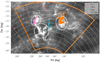 |
Fig. 1. Planck 857 GHz dust map of the Chamaeleon region. The positions of the main dark clouds are denoted with white ellipses. The area studied in this work is encompassed by the orange lines. The known members of Cha I and Cha II star-forming regions are shown as filled orange circles and pink crosses, respectively (Luhman 2007; Luhman & Muench 2008; Mužić et al. 2011; Sacco et al. 2017; Spezzi et al. 2008). The open cyan circles denote the ϵ Cha members (Murphy et al. 2013), and red diamonds are kinematic candidates associated with the A0 group of LCC from Goldman et al. (2018). |
Between the clouds (in projection), we find a more nearby (d ∼ 100 pc) and somewhat older (5–10 Myr) group of YSOs, known as the ϵ Chamaeleontis Association (ϵ Cha, Feigelson et al. 2003; Luhman et al. 2008; Dzib et al. 2018). Once thought to be the result of ejection from the Chamaeleon complex (Sterzik & Durisen 1995), many of these isolated, older pre-main-sequence stars are now believed to form a distinct nearby young co-moving group of ϵ Cha (Murphy et al. 2013).
One of the primary objectives of the survey presented in this paper is the extension of previous censuses of low-mass stars and substellar objects in Cha I, Cha II, and ϵ Cha. To achieve this, we use data from Gaia DR2 (Gaia Collaboration 2018). Gaia data has already been used in combination with near- and mid-infrared surveys to search for new low-mass stars and brown dwarfs in the solar neighbourhood (e.g., Esplin & Luhman 2019, Cánovas et al. 2019).
We confirmed the young age of candidate low-mass objects in Cha I, Cha II and ϵ Cha by performing optical spectroscopy. Analysing low-resolution optical spectra is not only a powerful tool to confirm the youth of low-mass stellar objects, but this method also useful to investigate their physical properties by comparing with spectra of standard stars with well-defined properties and templates. For nearby star-forming regions and associations, such observations can be performed with modest size telescopes. We performed spectroscopic follow-up using the Folded Low Order whYte-pupil Double-dispersed Spectrograph (FLOYDS) installed at the 2 m Faulkes South telescope, which is part of the Las Cumbres Observatory Global Network (LCOGT).
In this paper, we first describe the photometric datasets used for the analysis (Sect. 2) and introduce the known members (Sect. 2.4), followed by the selection of candidates from density maps, proper motions, and colour-magnitude diagrams (CMDs; Sect. 3). In Sect. 4, we present the analysis of the optical spectra. We then characterize the stellar parameters, spatial distribution, and spectral energy distributions (SEDs) of the confirmed members and summarize their properties. In the Appendix, we present the spectral template fits to the FLOYDS spectra obtained in this study.
2. Datasets
The region analysed in this work is located in the coordinate range 140° < α < 210° to −84° < δ < −73°. This large area, as shown in Fig. 1, encompasses the Chamaeleon clouds and the ϵ Cha moving group. The catalogues described in this section were cross-matched using TOPCAT (Taylor 2005) and have a matching radius of 1″.
2.1. Gaia DR2
The Gaia (Gaia Collaboration 2016) Data Release 2 (DR2; Gaia Collaboration 2018) catalogue of the region was queried through VizieR (Ochsenbein et al. 2000). The catalogue was restricted to parallaxes between 3.3 mas and 20 mas (equivalent to distances 50–300 pc) to reduce its size, but at the same time include the distances of interest with a generous margin. Furthermore, we excluded the objects with only one good observation, as reported by the catalogue keyword astrometric_n_good_obs_al.
2.2. 2MASS
The near-infrared photometry was obtained from the Two Micron All Sky Survey (2MASS; Skrutskie et al. 2006), queried through the Infrared Science Archive (IRSA) interface1. We kept only the photometric points with the quality flag (ph_qual) flag values of A, B, or C for any of the three 2MASS bands (J, H, and KS).
2.3. AllWISE
The mid-infared photometry (bands W1, W2, W3, and W4, centred at 3.6μm, 4.6μm, 11.6μm, and 22.1μm) was obtained from the AllWISE project, making use of data from the Wide-field Infrared Survey Explorer cryogenic survey (WISE; Wright et al. 2010). We filtered out the photometry for the bands with signal-to-noise ratio below 5 (keywords w1snr, w2snr, w3snr, and w4snr). Furthermore, the following flag values are accepted for W1 and W2 photometry: cc_flags = 0, ext_flg = 0–3, ph_qual = A or B, and w1flg = w2flg = 0.
2.4. Known members
The principal young populations known to be present towards the surveyed region are Cha I, Cha II, and ϵ Cha. In the north direction, at distances similar to ϵ Cha, we find Lower-Centaurus-Crux (LCC), which is part of the large-scale Sco-Cen OB association (de Zeeuw et al. 1999). In the original work by de Zeeuw et al. (1999) the LCC extends northward of the galactic longitude b > −10°, corresponding to δ ≳ −70°, that is outside the region studied in this work. The same is valid for the previous spectroscopic studies of the LCC candidate objects by Mamajek et al. (2002) and Song et al. (2012). However, a recent study based on Gaia DR2 astrometry (Goldman et al. 2018), searched for young sources over a slightly wider region, in which the authors subdivide the candidate members into four subgroups, which are characterised by the increasing isochronal age from 7 Myr to 10 Myr. The youngest group, labelled A0 by Goldman et al. (2018), partially overlaps with our search area and several of its candidate members were earlier recognised as members of ϵ Cha (Murphy et al. 2013). We denote the candidate members from Goldman et al. (2018) as LCC in Fig. 1, noting that some of these objects may as well be members of ϵ Cha. As we discuss in more detail later, the objects share the same proper motion and parallax space as well as the location in the barycentric Galactic Cartesian coordinate frame. For this reason as well, we do not use Goldman et al. candidates for the new member selection, we rather rely on ϵ Cha members, most of which were also confirmed by spectroscopy.
For our analysis, we take into account the following lists of members: (1) Cha I: A list of 256 spectroscopically confirmed members compiled using the works from Luhman (2007), Luhman & Muench (2008), Mužić et al. (2011), Sacco et al. (2017); (2) Cha II: A list of 51 spectroscopically confirmed members published in Spezzi et al. (2008); (3) ϵ Cha: A comprehensive list of 35 members compiled by Murphy et al. (2013), using kinematic and spectroscopic information. The previously confirmed members, along with the LCC (A0) candidates are shown in Fig. 1.
3. Candidate selection
3.1. On-sky density maps
To examine the large region shown in Fig 1, we first plotted stellar surface density maps limiting each map with a range of distances obtained from Gaia. The kernel density estimations (KDE) of the positions in the 2MASS J−band were plotted for the distance range of 50 pc–300 pc and have steps of 10 pc. The KDEs were obtained using a Gaussian kernel with a bandwidths of 25′, 25′, and 31′ for three-dimensions (RA, Dec, and parallax) for regions A to C, respectively2. This allowed us to visually identify stellar surface overdensities associated with the groups of interest in which we aim to select new candidates. After the visual inspection, we decided to focus on the following cubes, for which we investigated the most prominent stellar overdensities associated with regions:
-
Region A (associated with the Cha I cloud): 150° < α < 180° −79.5° < δ < −74.5° 4.75 mas < ϖ< 5.9 mas (≈170 pc < d < 210 pc)
-
Region B (associated with the Cha II cloud): 185° < α < 210° −79° < δ < −74° 4.55 mas < ϖ< 5.65 mas (≈180 pc < d < 220 pc)
-
Region C (in front of Chamaeleon clouds, associated with ϵ Cha and partially with LCC): 160° < α < 190° −82° < δ < −73° 8.3 mas < ϖ< 20 mas (≈50 pc < d < 120 pc).
The density maps showing these three regions are shown in Fig. 2, along with the known members described in Sect. 2.4.
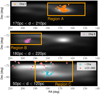 |
Fig. 2. J-band KDE maps for three different distance cuts. The three studied regions are denoted (see Sect. 3), along with the known members of various clusters and associations found in the area. The symbols are the same as in Fig. 1. |
The 3D areas from which regions A and B were selected overlap significantly; as shown in Fig. 2, the coordinate ranges are identical, but both cubes are slightly shifted in parallax range. We restricted our study to the vicinity of Cha II in the second 3D area (middle panel in Fig. 2), even though it is not visually the most prominent. The lower panel in Fig. 2 shows the most complex and extended enhancements in stellar densities. The two elongated overdensities are associated with previously identified young moving group ϵ Cha and recently postulated group A0 form LCC from Goldman et al. (2018). The two density enhancements seem to be separated by a strip of lower surface density. We discuss the relation between the two apparent structures in Sect. 5.1. The elongated shape of the overdensities is a projection effect owing to the large size of the region and its far south location as shown in Fig. 1. The purpose of presenting KDE maps in this work is only to guide our choice of the borders of regions (in α and δ) from which we aim to select new candidates.
3.2. Proper motion and colour selection
The left column of Fig. 3 exhibits the GBP − J, GBP CMDs for the three regions described in the previous section. The previously identified members of Cha I, Cha II, and ϵ Cha are located to the right of the main bulk of the sources, as expected from their pre-main-sequence status. These members are also clustered in the proper motion space (middle and right panels in Fig. 3). To select new candidates, we drew a line in the CMDs separating the field stars and the red photometric candidates, as well as an ellipse in the proper motion space, selected to encompass most of the known members. Our approach to the selection was conservative, aiming for a sample with fewer candidates, but with higher likelihood of membership. The exact functional forms are listed in the Appendix A. The sources that pass the two cuts, and are not on our previous member lists (Sect. 2.4), are considered new candidates for low-mass young members of Cha I, Cha II, ϵ Cha, or LCC. The total number of the new candidates is 35: 12 in region A, 4 in region B, and 19 in region C. All the new candidates are listed in Table 1 and shown in Fig. 4 and their membership status is discussed in more detail in the following sections.
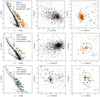 |
Fig. 3. Candidate selection based on colours and proper motions, with each row corresponding to one of the three regions of interest. The panels to the left show the GBP − J, GBP CMDs. The middle panels contain the proper motions; the red rectangle indicates the zoomed-in region of the plot, which is shown in the right-hand side panels. New candidates (green stars) are accepted if their colours and proper motions overlap with those of previously confirmed members (orange diamonds); that is sources are located to the right of the grey line in the panels to the left and inside the grey ellipse shown in the right-hand panels. Precise equations are listed in Appendix A. Photometric members with discrepant proper motions are indicated with blue crosses. The average proper motion uncertainties are shown in the lower right part of the zoomed-in proper motion plots; for region C these values were multiplied by 3 for better visibility. |
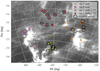 |
Fig. 4. Planck 857 GHz dust map of the Chamaeleon region, showing the candidates identified in this work. The black open circles denote those candidates for which we obtained spectra using FLOYDS spectrograph. |
New candidates.
3.3. Gaia eDR3
After the Gaia Early Data Release 3 (Gaia eDR3) on 3 December 2020 we repeated the candidate selection based on eDR3, applying the identical selection conditions as described in previous sections.
The list of selected candidates remains unchanged for Cha II and ϵ Cha, whereas one additional source passes our selection for the Cha I region. This source has coordinates α, δ = 11:19:36.44, −75:08:32.8; parallax and proper motions ϖ = 5.84 mas and (μα, μδ) = (−23.07, −1.10) mas yr−1. An improvement in the proper motion measurements in eDR3 causes the source to pass our selection criteria for the Cha I region. However, since the release of Gaia eDR3 occurred after the selection and analysis of the candidates and follow-up spectroscopy is already finished, we do not include this additional source in the analysis.
3.4. Spectral energy distributions
The SEDs were constructed using the photometry from Gaia, 2MASS, and WISE; the SED fitting was performed with the help of the Virtual Observatory SED Analyzer (VOSA; Bayo et al. 2008). The VOSA instrument takes the fluxes and distance for each object and looks for the best-fit effective temperature (Teff), fextinction (AV), and surface gravity (log g) by means of χ2 minimisation. For the objects showing excess in the WISE photometry, the SED fitting is performed over the optical and near-infrared portions of the SED. Otherwise the full available range is included in the fit. The metallicity was fixed to the solar value. We used the BT-Settl models (Allard et al. 2011) to probe Teff over the full range offered in VOSA (400–7000 K) with a step of 100 K, and AV between 0 and 5 mag with a step of 0.25 mag (automatically determined by VOSA). The only exception is the candidate #12, which is located in a small dusty cloud north-east of the main Cha I cloud and requires larger values of AV to be considered (AV = 0–10 mag). Furthermore, we allowed log g to vary between 3.5 and 5.0, which encompasses the typical ranges for young cool, very low-mass stars, brown dwarfs, and field stars. However, as previously noted by, for example Bayo et al. (2017), the SED fitting procedure is largely insensitive to log g, resulting in flat probability density distributions over the inspected range. Therefore the two main parameters constrained by this procedure are Teff and AV. The results of the SED fitting for all the candidates are given in the first three columns of Table 2, and are shown in Fig. 5.
 |
Fig. 5. Spectral energy distribution for all the identified candidates. The grey line shows the observed photometry. The filled circles connected with a grey line correspond to the observed photometry corrected from the best-fit value of the extinction, where the black circles are those used for the fitting, and the red circles were ignored owing to excess emission at these wavelengths. The orange diamonds represent the best-fitting BT-Settl model. |
Results of the spectral fitting, EWs, and membership assessment.
4. Spectroscopic follow-up and analysis
4.1. Observations and data reduction
Optical spectra of 18 low-mass candidates were taken using the FLOYDS spectrograph installed at the 2 m Faulkes South telescope, which is part of the Las Cumbres Observatory Global network (LCOGT). The priority in target selection was given to objects in region C, aiming to observe the faintest possible candidates, while maximising the efficiency and the total number of observed objects. At the end of the observing cycle we supplemented our target list by 4 candidates from region A in similar brightness range. The spectrograph provides a wide wavelength coverage of 3200–10 000 Å with a spectral resolution R ∼ 400−700. We set an upper wavelength cut-off at 9000 Å as a result of the strong telluric absorption present at longer wavelengths. Furthermore, we imposed a lower wavelength limit on a portion of our spectra owing to a very low signal-to-noise ratio (S/N) caused by the faintness of cool objects in the blue part of the spectrum. We employed a slit of 1.6″ and observed a flat field and an arc just before and after the science observations. For data reduction, we used the FLOYDS pipeline3, which performs overscan subtraction, flat fielding, defringing, cosmic-ray rejection, order rectification, spectral extraction, and flux and wavelength calibration. The list of the observed objects, along with the dates and exposure times, are given in Table 1. The data observed at two different dates for object #34 were combined to increase S/N, while we treat the two epochs of object #30 separately to analyse the strongly variable Hα emission. The candidates with spectra are denoted with black circles in Fig. 4.
4.2. Spectral type and extinction
The spectra in Fig. 6 clearly show that all the observed objects are cool dwarfs of spectral type M, dominated by various molecular features (mainly TiO and VO; Kirkpatrick et al. 1991, 1995). To derive more precise spectral types and assess if there is any extinction towards the objects, we compare the spectra to an empirical grid consisting of spectral templates:
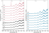 |
Fig. 6. Spectra towards the Chamaeleon region taken with the FLOYDS spectrograph. The spectra towards region A shown in black, and those from region C in pink (δ < −77°) and blue (δ > −77°). Two spectra are shown for object #30, taken at different dates. A strong variability in Hα emission can be appreciated. The region around ∼7600 Å has been masked owing to a pipeline artefact. The central wavelengths of Hα and Na I are indicated at the top of the figure. |
– Field: A grid of field dwarfs with spectral types M1–M9, separated by 0.5 spectral subtypes, was created by averaging a number of available spectra at each subtype4.
– Young: A grid of young objects (1–3 Myr) consists of the spectra of individual objects in Cha I, Taurus, η Cha (Luhman et al. 2003; Luhman 2004a,b,c), and Collinder 69 (Bayo et al. 2011) that have spectral types M1–M9 with a step of 0.25–0.5 spectral subtypes.
– TWA: Spectra of members of the TW Hydrae association (TWA) from Venuti et al. (2019), which have spectral type ranges M3–M5.5 and M8–M9.5 with a step of 0.5–1 spectral subtypes. The age of TWA (8–10 Myr; e.g., Ducourant et al. 2014; Herczeg & Hillenbrand 2014; Donaldson et al. 2016; Bell et al. 2015) make these spectra appropriate to compare with ϵ Cha, expected to be of similar age.
The template spectra were smoothed and rebinned to match the resolution and the wavelength scale of the FLOYDS spectra, and the region around the Hα line was masked (strong Hα may be present both in our spectra and the young templates, which may affect the fit). The spectral templates were reddened by AV = 0–5 mag, with a step of 0.2 mag, using the extinction law from Cardelli et al. (1989). The spectral fitting is performed over the wavelength range covered by the templates, typically 6100–9000 Å. The best-fit spectral type and extinction were determined by minimizing the reduced chi-squared value (χ2) defined as
 (1)
(1)
where O and σO are the object spectrum and its uncertainty, respectively, T the template spectrum, N the number of data points, and m the number of fitted parameters (m = 2).
An example of the best-fit spectra for each set of templates is shown in Fig. 7, for object #18. The remaining fits are shown in Figs. B.1 and B.2. Typically, several best-fit results cluster within ±1 spectral subtype or less, from the best-fit value, irrespective of the age of the objects in the template grid (field, TWA, or young). The extinction AV is zero, or very close to it, for all the objects. Of the 18 objects, 16 are best fit by either of the two younger categories (young or TWA), suggesting a young age for most of the objects. This, however, is not enough to claim youth for these objects, and the final membership assessment requires a closer look into gravity-sensitive spectral features. The derived spectral types and extinctions are given in Table 2.
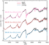 |
Fig. 7. Example of the spectral fitting for object #18 (black). The best-fit young (blue), TWA (red), and field (pink) template are shown, along with the corresponding spectral type, extinction, and the reduced χ2 of the fit. The TWA template provides the best fit to the overall spectrum and to the gravity sensitive sodium feature at ∼8200 Å. |
4.3. Indicators of youth and membership
As demonstrated in Fig. 6 of Mužić et al. (2014), optical spectra of M-dwarfs provide several gravity-sensitive features that allow us to distinguish young from the field stars, even at very low spectral resolution of a few hundred. The two main features that we rely on in this analysis are as follows: the Na I doublet at 8183/8195 Å, which becomes more pronounced (i.e. larger equivalent widths (EWs), and deeper absorption) at high surface gravities (e.g., Martín et al. 1999; Riddick et al. 2007; Schlieder et al. 2012); and the Hα emission, which is a sign of accretion and therefore youth.
Hα emission is commonly present in the spectra of M-type main-sequence stars as a result of a chromospheric activity, whereas in young stars both the activity and accretion may contribute. One way to identify the accreting sources is by means of elevated EWs of Hα with respect to non-accreting pre-main-sequence and main-sequence stars (White & Basri 2003; Barrado y Navascués & Martín 2003; Fang et al. 2009; Alonso-Floriano et al. 2015). We measured the pseudo-EWs5. The results are shown in Fig. 8 as a function of the spectral type. The error bars are calculated as standard deviations from repeated measurements obtained by slightly changing the wavelength range for the pseudo-continuum subtraction, and the range over which the EW is measured.
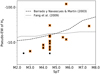 |
Fig. 8. Pseudo-EW measurement for the candidates with spectra (black dots). Two measurements for object #30, separated by about a month, are additionally denoted with open circles, and the objects with other signatures of youth (Na I doublet, X-ray detection or IR-excess) with orange crosses. The criteria separating the accretors from the non-accreting sources are shown by a dashed line (Barrado y Navascués & Martín 2003) and a dotted (Fang et al. 2009) line. |
The criteria used to distinguish between accretion and activity from Barrado y Navascués & Martín (2003) and Fang et al. (2009) are overplotted. Two sources are located above both lines (#22 and #30), while source #34 only passes the Fang et al. criterion. We note, however, that the equivalent plot from that work is more sparsely populated for spectral types later than M6 that of Barrado y Navascués & Martín (2003). Object #30 was observed twice and has about a month passing between the observations. The two measurements are highlighted with open circles in Fig. 8, one of which falls just below the accretion criterion. The continuum and emission line variability commonly occur in low-mass, pre-main-sequence stars (e.g., Nguyen et al. 2009). The Hα variability in several σ Ori (∼3 Myr) low-mass stars has been interpreted as consistent with the presence of cools spots with the filling factors between 0.2–0.4 (Bozhinova et al. 2016). Three more sources at the same spectral type as #30 (M4.5) fall close to it on its lower accretion levels (#20, #32, #35).
The strongest accreting object in our sample, candidate #22, has recently be reported by Schutte et al. (2020), who identify the object as a member of ϵ Cha, showing a strong infrared excess in the WISE data. The spectral type measured from the near-infrared spectra, M6±0.5, is in agreement with the spectral type found in this work.
We closely inspected all the spectra to identify the presence or absence of Hα emission and the strength of the Na I absorption. A dedicated column in Table 2 signals the presence of Hα, and a shallow Na I absorption, which we take as signatures of the young age of the source. The Na I criterion is stronger when assigning the membership to the sources because not all young stars may be accreting. Furthermore, the excess at mid-infrared wavelengths, signalling a presence of a disc or an envelope and strong X-ray emission, are well-established signatures of youth. Alcala et al. (1995) classified these X-ray emitters as WTTS based on presence of Li I (λ6707Å) absorption line and/or Hα emission line. The objects showing either of the two properties are additionally labelled as IRex or X in Table 2. Objects with one or more signatures of youth are considered members of the corresponding star-forming region or young moving group.
4.4. Comments on specific objects
A few of the objects on our candidate list, while not appearing on the member lists considered in Sect. 2.4, were studied in some detail in other works. We searched VizieR (Ochsenbein et al. 2000) and Simbad (Wenger et al. 2000) databases for additional information on the candidates.
Object #7 seems to be a known X-ray-emitting spectroscopic binary and a member of Cha I. Known also as RX J1108.8-7519A, it appears on members lists of Luhman et al. (2008) and Esplin et al. (2017) with a spectral type K6 and was classified as a WTTS by Wahhaj et al. (2010) and a Class III candidate by the machine learning classifier based on WISE photometry (Marton et al. 2016). Object #12 was previously identified as a Class I/II YSO candidate by Marton et al. (2016). Object #13 (AY Cha) was listed as a RR Lyrae variable in the General Catalogue of Variable Stars (Samus’ et al. 2017). It was also identified as a Class I/II YSO candidate by Marton et al. (2016); this is consistent with the SED (shown in Fig. 5), which clearly shows an infrared excess. Knowing that RR Lyrae are stars at a late stage of their evolution, typically associated with globular clusters and high galactic latitudes, we find this classification highly unlikely. We inspected the light curve from the Transiting Exoplanet Survey Satellite (TESS; Ricker et al. 2015). We find that the source shows a clear sinusoidal periodicity and does not show the characteristic RR Lyrae-type shape. We conclude that it is likely that this object is a young pre-main-sequence star. The objects #19, 26, and 27 were included in the list of provisional members of ϵ Cha in Murphy et al. (2013), pending further confirmation. Object #27 was classified as member by Feigelson et al. (2003) with the label ϵ Cha 12, but discarded by Murphy et al. (2013) as an outlier based on the proper motion measurements. The new astrometric information provided by Gaia speaks in favour of their membership, although none of these three objects were part of our spectroscopic follow-up.
4.5. Comparison to atmospheric models
In this section we use the FLOYDS spectra and apply χ2 minimisation to find the best-fit atmosphere model and its corresponding Teff, extinction AV, and log g. For this, we use the BT-Settl models (Allard et al. 2011) in the Teff range between 2000 K and 5000 K, in steps of 100 K and log g = 3.5–5.0 in steps of 0.5 dex. The AV is varied between 0 mag and 5 mag, with the step of 0.2 mag. As before, the extinction law from Cardelli et al. (1989) is employed to redden the models prior to χ2 calculation. The spectral fitting is performed over the full wavelength range of our spectra, from 5000 to 9000 Å. The best-fit parameters for each object are given in Table 2, and shown in Fig. 9. The fitting procedure is the same as in Sect. 3.4 but in this case performed on the optical spectra instead of the broad-band photometry. In both cases the selected models and parameter ranges are the same. In Sect. 3.4 the SED fitting is done for all selected candidates in Cha I, Cha II, and ϵ Cha; in this section we fit the parameters only for 18 sources with FLOYDS spectra.
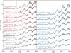 |
Fig. 9. Spectra of our candidates, along with the best-fit BT-Settl model. The models are colour-coded depending on the membership candidacy (grey for Cha I, red ϵ Cha, and blue ϵ Cha/LCC). |
While the overall shape of the spectra can be reasonably well represented by the models, the region around the Hα line does not match the shape of the spectra well. In any case, this region was excluded from the fitting procedure to avoid discrepancies due to Hα emission present in some of the candidate objects. The best-fit models show preference towards low surface gravity: 13/18 objects have log g = 3.5–4, which is characteristic for young low-mass stars and brown dwarfs. The remaining 5 objects have the best-fit log g = 4.5. The Teff and AV obtained by atmosphere model fitting tend to be systematically higher than those obtained both from the SED fitting (ΔTeff = 260 K, ΔAV = 1.5 mag on average) and the template fits (ΔAV = 1.7 mag). Most of our candidates are located in off-cloud regions, that is an extinction close to zero may be expected. A similar trend is present in the results of Bayo et al. (2017), when comparing the Teff and AV derived from fitting the BT-Settl models to the optical spectra and the SED fitting. On the other hand, these authors also report a trend towards determination of higher temperatures when using only optical data versus including the near-infrared spectra in the fit. In the latter case, the best-fit parameters are more in line with those from the SED fitting, which is probably not surprising given that the SEDs in Bayo et al. (2017) and in this work contain both optical and near-infrared photometry.
5. Discussion
5.1. Relation between ϵ Cha and LCC
Candidates from region C overlap with the proposed members of ϵ Cha (Murphy et al. 2013) and, towards the north, with the kinematic candidate members of the LCC A0 subgroup (Goldman et al. 2018). Moreover, there are several sources in common between the two lists. As already pointed out by Murphy et al. (2013), given the similarity in ages, kinematics, distances, and the observed trends in these parameters, a useful demarcation between the southern extent of LCC and ϵ Cha may simply not exist. In this section we try to shed some light on the relation between these two regions, based on the improved astrometry provided by Gaia DR2.
As evident from the surface density plots (Fig. 2), there appears to be a gap between the region where the main bulk of ϵ Cha members reside and the northern portion where the LCC candidates overlap with a smaller portion of the ϵ Cha objects. To investigate the properties of our region C candidates associated with the two overdensities observed in Fig. 2, we divide sources according to the declination, as those south or north of δ = 77°. These are plotted as red and green stars in Fig. 10, in which we show their on-sky positions and Gaia DR2 proper motions, along with the members of ϵ Cha and LCC candidates. The latter are colour-coded according to declination (top plots) and distance (bottom). The LCC candidates show a clear gradient in proper motions both with the on-sky position and with the distance. Both ϵ Cha members and our objects share the proper motion space with the southern-most subgroup of LCC (A0), and cannot be separated either according to the proper motion or the distance. The mean values and the standard deviations of these quantities are as follows:
-
Candidates with δ < −77° (southern portion): μα cos δ = −40.73 ± 1.35 mas yr−1, μδ = −6.14 ± 0.80 mas yr−1, ϖ = 9.58 ± 0.29 mas.
-
Candidates with δ > −77° (northern portion): μα cos δ = −40.32 ± 1.39 mas yr−1, μδ = −7.24 ± 2.04 mas yr−1, ϖ = 9.80 ± 0.39 mas.
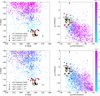 |
Fig. 10. On-sky positions and proper motions of the candidates from region C (red and green stars), along with the members ϵ Cha (black circles Murphy et al. 2013) and Gaia DR2-selected candidate members of LCC (coloured dots Goldman et al. 2018). The LCC sources are coloured according to the declination (top plots) and Gaia DR2 distance (bottom). The distances of ϵ Cha objects in this plot are in the range ∼93–110 pc, similar to our candidates (∼94–113 pc). |
To try to understand better the relation of our candidates with the two structures as per their positions in the Galaxy, in Fig. 11, we show their distribution in the Galactic XYZ coordinate frame, with the axes pointing towards the Galactic centre (X), in the direction of the Galactic rotation (Y), and towards the north Galactic pole (Z). Furthermore, we plot the space occupied by ϵ Cha and LCC according to the BANYAN kinematic models of the nearby moving groups (shaded ellipses; Gagné et al. 2018), and the LCC subgroups A0, A, B, and C from Goldman et al. (2018). While in the XY plane (left panel in Fig. 11) all of the structures show a significant overlap, there is a clear distinction between several structures perpendicular to the Galactic plane. The BANYAN definition of LCC overlaps with the Goldman groups A, B, and C, whereas the A0 group appears as a bridge between those groups and ϵ Cha. According to the BANYAN Σ tool (Gagné et al. 2018), all our candidates have a high probability of being members of ϵ Cha, but the probability of belonging to LCC is mostly non-existent; the reason for this is evident from Fig. 11. Candidate #17 has an 87.5% probability of belonging to ϵ Cha, 8.2% to LCC, and 4.3% to the field. All the remaining candidates have ≳97% probability of belonging to ϵ Cha. The Bayesian probabilities reported by BANYAN Σ are designed to generate recovery rates of 82% when proper motion and distance are used, and 90% when proper motion, radial velocity, and distance are used. Of the 19 region C candidates, 3 have the radial velocities reported in the literature. The age of ϵ Cha derived by Murphy et al. (2013) is 3.7 Myrs, whereas Goldman et al. show the age distribution of A0 that peaks at ∼7 Myr, but extends from ∼3 yr to > 10 Myr. Given both the statistical uncertainties of these estimates, as well as the systematics associated with age derivation from the Hertzsprung Russell (HR) diagrams (the uncertainties in distances and bolometric corrections and the use of different sets of evolutionary models in the two works), these two estimates are basically indistinguishable. The same is true for the two spatial subgroups of region C defined by the dividing line δ = −77°, where the northern subgroup has the mean age determined from the HR diagram (Fig. 12) of 7 ± 5 Myr, and the southern subgroup 6 ± 3 Myr. To conclude, given the present evidence on the age, parallax, proper motions, and the position in the Galaxy, it cannot be excluded that ϵ Cha and the southern extension of the LCC (A0) may have been born during the same star formation event.
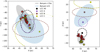 |
Fig. 11. Distribution of the region C candidates in the Galactic XYZ coordinates, where the positive X axis points towards the Galactic centre, Y is in the direction of the Galactic rotation, and Z points towards the north Galactic pole. The candidates are represented by stars, with the colour-coding identical to that of Fig. 10. The shaded ellipses denote the areas occupied by ϵ Cha and LCC members from the BANYAN Σ model (Gagné et al. 2018). The dots indicate the mean positions of the LCC subgroups and the semi-major or minor axes of the dashed ellipses equal 2 standard deviations (Goldman et al. 2018). |
5.2. Hertzsprung-Russell diagram
To construct the HR diagram shown in Fig. 12, we use the Teff and log L determined by VOSA SED fitting. The bolometric luminosity is calculated from the total observed flux, which VOSA determines by integrating the best-fit model, multiplied by the dilution factor (R/d)2, where R is the radius estimated in the fitting process and d is the distance. All 35 candidates are shown in Fig. 12, along with the isochrones (1–30 Myr) and the lines of constant mass from the BT-Settl series. The candidates belonging to region B (Cha II) appear the youngest of the whole sample (≲1 Myr), which is corroborated by the IR excess exhibited by two of objects. The Region A (Cha I) candidates are mostly consistent with ages ≲5 Myr and have a mean age of 3 ± 2 Myr. The Region C is the oldest and has a mean age of 6 ± 4 Myr. This is consistent with the results from fitting spectral templates. In most cases the best-fitting spectral template is from objects in the TW Hya association, indicating that ϵ Cha has a similar age. There is no significant age difference between candidates from the northern (age of 7 ± 5 Myr) and southern (age of 6 ± 3 Myr) part of the region.
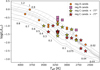 |
Fig. 12. Hertzsprung-Russell diagram for the candidates, along with the BT-Settl isochrones (solid lines) and the lines of constant mass (dotted lines). The isochrones correspond to the ages (1, 2, 3, 4, 5 (darker line), 10, 20, 30) Myr, from top to bottom, and the masses are given in M⊙. The uncertainties in Teff are 100 K, reflecting the spacing of the grid, while those in log L are comparable to or smaller than the symbol sizes. |
5.3. Updated census in ϵ Cha and the IMF
Murphy et al. (2013) compiled a list of 35 members of ϵ Cha based on common kinematics. Our selection yields additional 18 candidates, of which 14 are included in the spectroscopic follow-up; 13 of these are confirmed as young sources. Additionally, sources #19 and #24 are X-ray emitters, which indicates their youth. Our study increases the census of confirmed members of ϵ Cha by 15 new members, which is 43% more. Out of 14 sources for which we obtained spectra, only one seems to belong to the field (see Fig. B.2), that is the confirmation rate of our selection method is larger than 90%. For this reason, we included all of our candidates except that one rejected source in the sample used to calculate the initial mass function (IMF). The final sample for the IMF therefore contains the previously known, confirmed, and candidate members, which is in total 52 objects.
The spectral types obtained from spectral fitting indicate that only one member of ϵ Cha (source #34) is a brown dwarf, which has the latest spectral type of M7.5. All except one member have spectral types later than M4.5. Our spectral fitting was done with steps of 0.5–1 subtypes (see Sect. 4.2). Recently source #20 has been reported by Schutte et al. (2020), who identify the object as accreting brown dwarf with spectral type of M6 ± 0.5 based on infrared spectra. Our fit to optical templates results in spectral type M4.5 ± 1. Taking this into account together with the positions of all sources in the HR diagram, our selection contains 3 brown dwarfs in Cha I and 5 brown dwarfs in ϵ Cha. The IMF estimation for ϵ Cha presented below is to the best of our knowledge the first time reaching the substellar mass regime for this young moving group.
We obtained a mass distribution for each of the objects by running VOSA on 100 different photometry sets. In each realisation the photometry is moved by a random offset within the respective photometry errors (assuming Gaussian distributions). It is worth mentioning that VOSA did not produce results (mass and/or age) in some runs, if the source lies outside the area covered by the isochrones in HR diagram. In order to obtain an evenly sampled mass distribution, we ran a Monte Carlo simulation for each of the 52 sources. The Monte Carlo simulation is very similar to that previously applied by Mužić et al. (2019). The mass of each star is drawn from the distribution derived by multiple realisations of VOSA. This is performed 100 times and for each of the 100 realisations we do 100 bootstraps, that is random samplings with replacement. In other words, starting from a sample with N ≤ 100 members, in each bootstrap we draw a new sample of 100 members, allowing some members of the initial sample to be drawn multiple times. This results in 104 samples of the mass distributions for each star, which are used to derive dN/dM and the corresponding uncertainties.
In Fig. 13, we show the IMF and the corresponding fits in the power-law form dN/dM ∝ M−α. The IMF can be represented by two power laws with a break around 0.5 M⊙. For M < 0.5 M⊙ α = 0.42 ± 0.11 and for M > 0.5 M⊙ α = 1.44 ± 0.12. Both values are in agreement with the power-law slope of low-mass IMF in various star-forming regions (cf. Table 4 in Mužić et al. (2017)). This IMF estimation is only illustrative since the membership of ϵ Cha is still not complete, especially in the substellar regime.
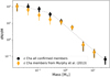 |
Fig. 13. Initial mass function of the ϵ Cha updated census, represented in equal-size bins of 0.2 dex in mass. The results are plotted from Monte Carlo simulations of mass distribution and corresponding uncertainties. The distribution from updated census is shown in black, and the distribution based on Murphy et al. (2013) our membership is shown in yellow. |
We estimate the completeness of the spectroscopically observed sample in ϵ Cha to be GBP = 18.5 mag. Photometry reaches fainter stars when compared to spectroscopy. We estimate the completeness of photometric data used in our selection to be two magnitudes deeper, GBP = 20.5 mag. This corresponds to a mass of M = 0.02−0.03 M⊙ for an age of 5 Myrs. Additionally we do not take into account any information about multiplicity of the objects, even though the majority of the members selected in Murphy et al. (2013) are known to be spectroscopic binaries.
5.4. Distance to ϵ Cha
The distance to ϵ Cha was estimated based on Gaia DR2 data, in a way similar to Mužić et al. (2019). We used a maximum-likelihood procedure (Cantat-Gaudin et al. 2018), maximising the following quantity:
 (2)
(2)
where P(ϖ|d, σϖi) is the probability of measuring a value ϖi for the parallax of star i, if its true distance is d and its measurement uncertainty is σϖi. This approach neglects correlations between parallax measurements of all stars and considers the likelihood for the ϵ Cha distance to be the product of the individual likelihoods of its members.
First we checked the distance to the ϵ Cha moving group based on known members. Out of 35 stars confirmed by Murphy et al. (2013), 32 have distances in the Gaia DR2 catalogue (1″ matching radius). The three missing objects are members of multiple systems (HD104237 B and C, and ϵ Cha AB). Additionally, the parallaxes for two sources are much smaller than the average parallax for the sample (mean ϖ = 9.61 mas, with a standard deviation of 1.00 mas; mean errors σϖ = 0.10 mas, with a standard deviation of 0.15 mas). For 2MASS J11432669-7804454 (eps Cha 17 from Feigelson et al. 2003), the parallax is ϖ = 5.548 ± 0.562 mas (d ≈ 181 ± 18 pc) and the parallax of RX J1220.4-7407 (eps Cha 36 in Feigelson et al. 2003) is ϖ = 6.714 ± 0.698 mas (d ≈ 149 ± 15 pc). Including these sources in the distance estimation does not change the result significantly, nevertheless we suggest re-examining their membership. We obtained a distance of d = 102.2 ± 0.4 pc when using only members from Murphy et al. (2013). When combining with confirmed members from our study, the distance is 102.5 ± 0.6 pc. The new distance estimate is somewhat lower than the kinematic distance estimated by Murphy et al. (2013) (110 ± 7 pc), but these estimates agree within the errors.
6. Conclusions
In this work we take advantage of Gaia DR2 data to investigate the Chamaeleon complex and its projected surroundings. From the optical and near-infrared photometry, we selected 35 objects as candidate members for Cha I (12 candidates), Cha II (4 candidates), and ϵ Cha (18 candidates). We obtained low-resolution optical spectra for 18 of our candidates, 4 in Cha I, and 14 in ϵ Cha. Among these we confirmed the young evolutionary stage of 16 candidates.
From Murphy et al. (2013) we know the membership of 35 objects in ϵ Cha, confirmed based on their kinematics and spectroscopy. We confirmed 13 new members spectroscopically and rely on X-ray emission as youth indicator for 2 more. These 15 new members increase the census of ϵ Cha by 43%. Our spectral fits and the location in the HR diagram show that the new members of the ϵ Cha moving group have a similar age as the TW Hydrae association (8–10 Myr; e.g., Ducourant et al. 2014).
Unfortunately, the significant increase in statistics does not help to improve our understanding of the origin of ϵ Cha and LCC. Murphy et al. (2013) already pointed out that with the given similarity in ages, kinematics, and distances, a simple and obvious separation between LCC and ϵ Cha may not be possible. ϵ Cha and LCC A0, the southernmost group of LCC, occupy the same proper motion space and also cannot be distinguished in distance. The two density enhancements seem to be separated by a strip of lower surface density (see Fig. 2).
However, there is a pattern of several structures from LCC sub-populations (A, B, C; Goldman et al. 2018) and ϵ Cha perpendicular to the Galactic plane (based on BANYAN Σ model; Gagné et al. 2018, see Fig. 11). Since the LCC A0 group appears as a bridge between those groups and ϵ Cha, they may have been born during the same star formation event.
The lower density at the edges of the plots is an artefact. The KDE sums Gaussian contributions from each star and regions close to the edges miss the contribution from the sources located beyond them.
The EW, with respect to a local pseudo-continuum, that is formed by molecular band absorptions dominating the optical spectra of cool dwarfs.
Acknowledgments
We would like to thank the anonymous referee for their valuable comments that helped improve the manuscript. K. K., K. M., and V. A-A. acknowledge funding by the Science and Technology Foundation of Portugal (FCT), Grants No. IF/00194/2015, PTDC/FIS-AST/28731/2017, UIDB/00099/2020, and SFRH/BD/143433/2019. This publication makes use of VOSA, developed under the Spanish Virtual Observatory project supported by the Spanish MINECO through grant AyA2017-84089. VOSA has been partially updated by using funding from the European Union’s Horizon 2020 Research and Innovation Programme, under Grant Agreement no. 776403 (EXOPLANETS-A).
References
- Alcala, J. M., Krautter, J., Schmitt, J. H. M. M., et al. 1995, A&AS, 114, 109 [NASA ADS] [Google Scholar]
- Allard, F., Homeier, D., & Freytag, B. 2011, in 16th Cambridge Workshop on Cool Stars, Stellar Systems, and the Sun, eds. C. Johns-Krull, M. K. Browning, & A. A. West, ASP Conf. Ser., 448, 91 [Google Scholar]
- Alonso-Floriano, F. J., Morales, J. C., Caballero, J. A., et al. 2015, A&A, 577, A128 [NASA ADS] [CrossRef] [EDP Sciences] [Google Scholar]
- Barrado y Navascués, D., & Martín, E. L. 2003, AJ, 126, 2997 [Google Scholar]
- Bayo, A., Rodrigo, C., Barrado Y Navascués, D., et al. 2008, A&A, 492, 277 [NASA ADS] [CrossRef] [EDP Sciences] [Google Scholar]
- Bayo, A., Barrado, D., Stauffer, J., et al. 2011, A&A, 536, A63 [NASA ADS] [CrossRef] [EDP Sciences] [Google Scholar]
- Bayo, A., Barrado, D., Allard, F., et al. 2017, MNRAS, 465, 760 [Google Scholar]
- Bell, C. P. M., Mamajek, E. E., & Naylor, T. 2015, MNRAS, 454, 593 [NASA ADS] [CrossRef] [Google Scholar]
- Bozhinova, I., Scholz, A., & Eislöffel, J. 2016, MNRAS, 458, 3118 [Google Scholar]
- Cánovas, H., Cantero, C., Cieza, L., et al. 2019, A&A, 626, A80 [NASA ADS] [CrossRef] [EDP Sciences] [Google Scholar]
- Cantat-Gaudin, T., Jordi, C., Vallenari, A., et al. 2018, A&A, 618, A93 [NASA ADS] [CrossRef] [EDP Sciences] [Google Scholar]
- Cardelli, J. A., Clayton, G. C., & Mathis, J. S. 1989, ApJ, 345, 245 [NASA ADS] [CrossRef] [Google Scholar]
- de Zeeuw, P. T., Hoogerwerf, R., de Bruijne, J. H. J., Brown, A. G. A., & Blaauw, A. 1999, AJ, 117, 354 [NASA ADS] [CrossRef] [Google Scholar]
- Donaldson, J. K., Weinberger, A. J., Gagné, J., et al. 2016, ApJ, 833, 95 [Google Scholar]
- Ducourant, C., Teixeira, R., Galli, P. A. B., et al. 2014, A&A, 563, A121 [NASA ADS] [CrossRef] [EDP Sciences] [Google Scholar]
- Dzib, S. A., Loinard, L., Ortiz-León, G. N., Rodríguez, L. F., & Galli, P. A. B. 2018, ApJ, 867, 151 [NASA ADS] [CrossRef] [Google Scholar]
- Esplin, T. L., & Luhman, K. L. 2019, AJ, 158, 54 [Google Scholar]
- Esplin, T. L., Luhman, K. L., Faherty, J. K., Mamajek, E. E., & Bochanski, J. J. 2017, AJ, 154, 46 [NASA ADS] [CrossRef] [Google Scholar]
- Fang, M., van Boekel, R., Wang, W., et al. 2009, A&A, 504, 461 [NASA ADS] [CrossRef] [EDP Sciences] [Google Scholar]
- Feigelson, E. D., Lawson, W. A., & Garmire, G. P. 2003, ApJ, 599, 1207 [Google Scholar]
- Gagné, J., Mamajek, E. E., Malo, L., et al. 2018, ApJ, 856, 23 [NASA ADS] [CrossRef] [Google Scholar]
- Gaia Collaboration (Prusti, T., et al.) 2016, A&A, 595, A1 [NASA ADS] [CrossRef] [EDP Sciences] [Google Scholar]
- Gaia Collaboration (Brown, A. G. A., et al.) 2018, A&A, 616, A1 [NASA ADS] [CrossRef] [EDP Sciences] [Google Scholar]
- Goldman, B., Röser, S., Schilbach, E., Moór, A. C., & Henning, T. 2018, ApJ, 868, 32 [Google Scholar]
- Herczeg, G. J., & Hillenbrand, L. A. 2014, ApJ, 786, 97 [Google Scholar]
- Kirkpatrick, J. D., Henry, T. J., & McCarthy, D. W., Jr 1991, ApJS, 77, 417 [Google Scholar]
- Kirkpatrick, J. D., Henry, T. J., & Simons, D. A. 1995, AJ, 109, 797 [Google Scholar]
- Luhman, K. L. 2004a, ApJ, 602, 816 [NASA ADS] [CrossRef] [Google Scholar]
- Luhman, K. L. 2004b, ApJ, 616, 1033 [Google Scholar]
- Luhman, K. L. 2004c, ApJ, 617, 1216 [Google Scholar]
- Luhman, K. L. 2007, ApJS, 173, 104 [NASA ADS] [CrossRef] [Google Scholar]
- Luhman, K. L., & Muench, A. A. 2008, ApJ, 684, 654 [Google Scholar]
- Luhman, K. L., Briceño, C., Stauffer, J. R., et al. 2003, ApJ, 590, 348 [Google Scholar]
- Luhman, K. L., Allen, L. E., Allen, P. R., et al. 2008, ApJ, 675, 1375 [NASA ADS] [CrossRef] [Google Scholar]
- Mamajek, E. E., Meyer, M. R., & Liebert, J. 2002, AJ, 124, 1670 [Google Scholar]
- Martín, E. L., Delfosse, X., Basri, G., et al. 1999, AJ, 118, 2466 [Google Scholar]
- Marton, G., Tóth, L. V., Paladini, R., et al. 2016, MNRAS, 458, 3479 [NASA ADS] [CrossRef] [Google Scholar]
- Murphy, S. J., Lawson, W. A., & Bessell, M. S. 2013, MNRAS, 435, 1325 [NASA ADS] [CrossRef] [Google Scholar]
- Mužić, K., Scholz, A., Geers, V., Fissel, L., & Jayawardhana, R. 2011, ApJ, 732, 86 [Google Scholar]
- Mužić, K., Scholz, A., Geers, V. C., Jayawardhana, R., & López Martí, B. 2014, ApJ, 785, 159 [Google Scholar]
- Mužić, K., Schödel, R., Scholz, A. E., et al. 2017, MNRAS, 471, 3699 [Google Scholar]
- Mužić, K., Scholz, A., Peña Ramírez, K., et al. 2019, ApJ, 881, 79 [Google Scholar]
- Nguyen, D. C., Scholz, A., van Kerkwijk, M. H., Jayawardhana, R., & Brandeker, A. 2009, ApJ, 694, L153 [Google Scholar]
- Ochsenbein, F., Bauer, P., & Marcout, J. 2000, A&AS, 143, 23 [NASA ADS] [CrossRef] [EDP Sciences] [Google Scholar]
- Ricker, G. R., Winn, J. N., Vanderspek, R., et al. 2015, J. Astron. Telesc. Instrum. Syst., 1, 014003 [Google Scholar]
- Riddick, F. C., Roche, P. F., & Lucas, P. W. 2007, MNRAS, 381, 1067 [Google Scholar]
- Sacco, G. G., Spina, L., Randich, S., et al. 2017, A&A, 601, A97 [NASA ADS] [CrossRef] [EDP Sciences] [Google Scholar]
- Samus’, N. N., Kazarovets, E. V., Durlevich, O. V., Kireeva, N. N., & Pastukhova, E. N. 2017, Astron. Rep., 61, 80 [NASA ADS] [CrossRef] [Google Scholar]
- Schlieder, J. E., Lépine, S., & Simon, M. 2012, AJ, 144, 109 [Google Scholar]
- Schutte, M. C., Lawson, K. D., Wisniewski, J. P., et al. 2020, AJ, 160, 156 [Google Scholar]
- Skrutskie, M. F., Cutri, R. M., Stiening, R., et al. 2006, AJ, 131, 1163 [NASA ADS] [CrossRef] [Google Scholar]
- Song, I., Zuckerman, B., & Bessell, M. S. 2012, AJ, 144, 8 [Google Scholar]
- Spezzi, L., Alcalá, J. M., Covino, E., et al. 2008, ApJ, 680, 1295 [NASA ADS] [CrossRef] [Google Scholar]
- Sterzik, M. F., & Durisen, R. H. 1995, A&A, 304, L9 [NASA ADS] [Google Scholar]
- Taylor, M. B. 2005, Astronomical Data Analysis Software and Systems XIV, eds. P. Shopbell, M. Britton, & R. Ebert, ASP Conf. Ser., 347, 29 [Google Scholar]
- Venuti, L., Stelzer, B., Alcalá, J. M., et al. 2019, A&A, 632, A46 [CrossRef] [EDP Sciences] [Google Scholar]
- Wahhaj, Z., Cieza, L., Koerner, D. W., et al. 2010, ApJ, 724, 835 [Google Scholar]
- Wenger, M., Ochsenbein, F., Egret, D., et al. 2000, A&AS, 143, 9 [NASA ADS] [CrossRef] [EDP Sciences] [Google Scholar]
- White, R. J., & Basri, G. 2003, ApJ, 582, 1109 [NASA ADS] [CrossRef] [Google Scholar]
- Wright, E. L., Eisenhardt, P. R. M., Mainzer, A. K., et al. 2010, AJ, 140, 1868 [Google Scholar]
- Zucker, C., Speagle, J. S., Schlafly, E. F., et al. 2020, A&A, 633, A51 [CrossRef] [EDP Sciences] [Google Scholar]
Appendix A: Candidate selection criteria
Functional forms for the candidates selection criteria presented in Fig. 3.
Selection criteria used in this work.
Appendix B: Spectral template fits
In Figs. B.1 and B.2 we show the remaining spectral template fits described in Sect. 4.2.
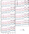 |
Fig. B.1. Spectral fitting results for the candidate objects in regions A and C (southern portion). The observed spectra are shown in black. The best-fit young (blue), TWA (red), and field (pink) template are shown, along with the corresponding spectral type, extinction, and the reduced χ2 of the fit. The Hα emission in some of the template spectra is masked. All the spectra are scaled at 7500 Å and offset for clarity. |
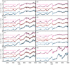 |
Fig. B.2. Spectral fitting results for the candidate objects in the northern portion of region C. The observed spectra are shown in black. The best-fit young (blue), TWA (red), and field (pink) template are shown, along with the corresponding spectral type, extinction, and the reduced χ2 of the fit. The Hα emission in some of the template spectra is masked. All the spectra are scaled at 7500 Å and offset for clarity. For object #34 we do not show the best-fit TWA template, since the grid is missing spectral types in the range M6–M7.5, inclusive, which coincides with the probable spectral type of the object. |
All Tables
All Figures
|
Fig. 1. Planck 857 GHz dust map of the Chamaeleon region. The positions of the main dark clouds are denoted with white ellipses. The area studied in this work is encompassed by the orange lines. The known members of Cha I and Cha II star-forming regions are shown as filled orange circles and pink crosses, respectively (Luhman 2007; Luhman & Muench 2008; Mužić et al. 2011; Sacco et al. 2017; Spezzi et al. 2008). The open cyan circles denote the ϵ Cha members (Murphy et al. 2013), and red diamonds are kinematic candidates associated with the A0 group of LCC from Goldman et al. (2018). |
| In the text | |
|
Fig. 2. J-band KDE maps for three different distance cuts. The three studied regions are denoted (see Sect. 3), along with the known members of various clusters and associations found in the area. The symbols are the same as in Fig. 1. |
| In the text | |
|
Fig. 3. Candidate selection based on colours and proper motions, with each row corresponding to one of the three regions of interest. The panels to the left show the GBP − J, GBP CMDs. The middle panels contain the proper motions; the red rectangle indicates the zoomed-in region of the plot, which is shown in the right-hand side panels. New candidates (green stars) are accepted if their colours and proper motions overlap with those of previously confirmed members (orange diamonds); that is sources are located to the right of the grey line in the panels to the left and inside the grey ellipse shown in the right-hand panels. Precise equations are listed in Appendix A. Photometric members with discrepant proper motions are indicated with blue crosses. The average proper motion uncertainties are shown in the lower right part of the zoomed-in proper motion plots; for region C these values were multiplied by 3 for better visibility. |
| In the text | |
|
Fig. 4. Planck 857 GHz dust map of the Chamaeleon region, showing the candidates identified in this work. The black open circles denote those candidates for which we obtained spectra using FLOYDS spectrograph. |
| In the text | |
|
Fig. 5. Spectral energy distribution for all the identified candidates. The grey line shows the observed photometry. The filled circles connected with a grey line correspond to the observed photometry corrected from the best-fit value of the extinction, where the black circles are those used for the fitting, and the red circles were ignored owing to excess emission at these wavelengths. The orange diamonds represent the best-fitting BT-Settl model. |
| In the text | |
|
Fig. 6. Spectra towards the Chamaeleon region taken with the FLOYDS spectrograph. The spectra towards region A shown in black, and those from region C in pink (δ < −77°) and blue (δ > −77°). Two spectra are shown for object #30, taken at different dates. A strong variability in Hα emission can be appreciated. The region around ∼7600 Å has been masked owing to a pipeline artefact. The central wavelengths of Hα and Na I are indicated at the top of the figure. |
| In the text | |
|
Fig. 7. Example of the spectral fitting for object #18 (black). The best-fit young (blue), TWA (red), and field (pink) template are shown, along with the corresponding spectral type, extinction, and the reduced χ2 of the fit. The TWA template provides the best fit to the overall spectrum and to the gravity sensitive sodium feature at ∼8200 Å. |
| In the text | |
|
Fig. 8. Pseudo-EW measurement for the candidates with spectra (black dots). Two measurements for object #30, separated by about a month, are additionally denoted with open circles, and the objects with other signatures of youth (Na I doublet, X-ray detection or IR-excess) with orange crosses. The criteria separating the accretors from the non-accreting sources are shown by a dashed line (Barrado y Navascués & Martín 2003) and a dotted (Fang et al. 2009) line. |
| In the text | |
|
Fig. 9. Spectra of our candidates, along with the best-fit BT-Settl model. The models are colour-coded depending on the membership candidacy (grey for Cha I, red ϵ Cha, and blue ϵ Cha/LCC). |
| In the text | |
|
Fig. 10. On-sky positions and proper motions of the candidates from region C (red and green stars), along with the members ϵ Cha (black circles Murphy et al. 2013) and Gaia DR2-selected candidate members of LCC (coloured dots Goldman et al. 2018). The LCC sources are coloured according to the declination (top plots) and Gaia DR2 distance (bottom). The distances of ϵ Cha objects in this plot are in the range ∼93–110 pc, similar to our candidates (∼94–113 pc). |
| In the text | |
|
Fig. 11. Distribution of the region C candidates in the Galactic XYZ coordinates, where the positive X axis points towards the Galactic centre, Y is in the direction of the Galactic rotation, and Z points towards the north Galactic pole. The candidates are represented by stars, with the colour-coding identical to that of Fig. 10. The shaded ellipses denote the areas occupied by ϵ Cha and LCC members from the BANYAN Σ model (Gagné et al. 2018). The dots indicate the mean positions of the LCC subgroups and the semi-major or minor axes of the dashed ellipses equal 2 standard deviations (Goldman et al. 2018). |
| In the text | |
|
Fig. 12. Hertzsprung-Russell diagram for the candidates, along with the BT-Settl isochrones (solid lines) and the lines of constant mass (dotted lines). The isochrones correspond to the ages (1, 2, 3, 4, 5 (darker line), 10, 20, 30) Myr, from top to bottom, and the masses are given in M⊙. The uncertainties in Teff are 100 K, reflecting the spacing of the grid, while those in log L are comparable to or smaller than the symbol sizes. |
| In the text | |
|
Fig. 13. Initial mass function of the ϵ Cha updated census, represented in equal-size bins of 0.2 dex in mass. The results are plotted from Monte Carlo simulations of mass distribution and corresponding uncertainties. The distribution from updated census is shown in black, and the distribution based on Murphy et al. (2013) our membership is shown in yellow. |
| In the text | |
|
Fig. B.1. Spectral fitting results for the candidate objects in regions A and C (southern portion). The observed spectra are shown in black. The best-fit young (blue), TWA (red), and field (pink) template are shown, along with the corresponding spectral type, extinction, and the reduced χ2 of the fit. The Hα emission in some of the template spectra is masked. All the spectra are scaled at 7500 Å and offset for clarity. |
| In the text | |
|
Fig. B.2. Spectral fitting results for the candidate objects in the northern portion of region C. The observed spectra are shown in black. The best-fit young (blue), TWA (red), and field (pink) template are shown, along with the corresponding spectral type, extinction, and the reduced χ2 of the fit. The Hα emission in some of the template spectra is masked. All the spectra are scaled at 7500 Å and offset for clarity. For object #34 we do not show the best-fit TWA template, since the grid is missing spectral types in the range M6–M7.5, inclusive, which coincides with the probable spectral type of the object. |
| In the text | |
Current usage metrics show cumulative count of Article Views (full-text article views including HTML views, PDF and ePub downloads, according to the available data) and Abstracts Views on Vision4Press platform.
Data correspond to usage on the plateform after 2015. The current usage metrics is available 48-96 hours after online publication and is updated daily on week days.
Initial download of the metrics may take a while.