| Issue |
A&A
Volume 649, May 2021
|
|
|---|---|---|
| Article Number | A28 | |
| Number of page(s) | 15 | |
| Section | Stellar structure and evolution | |
| DOI | https://doi.org/10.1051/0004-6361/202040050 | |
| Published online | 06 May 2021 | |
The aftermath of nova Centauri 2013 (V1369 Centauri)
1
INAF-OATS, Via G.B. Tiepolo 11, 34143 Trieste, Italy
e-mail: This email address is being protected from spambots. You need JavaScript enabled to view it.
2
Dipartimento di Fisica “Enrico Fermi”, Università di Pisa & INFN-Pisa, Largo Pontecorvo 3, 56127 Pisa, Italy
3
Smithsonian Astrophysical Observatory, MS-03, 60 Garden Street, Cambridge, MA 02138, USA
4
Space Science and Astrobiology Division, NASA Ames Research Center, M/S 245-6, Moffett Field, CA 94035, USA
5
Mullard Space Science Laboratory, University College London, Holmbury St Mary, Dorking, Surrey RH5 6NT, UK
6
Institut für Astronomie & Astrophysik, Eberhard Karls Universität Tübingen, Geschwister-Scholl-Platz, 72074 Tübingen, Germany
Received:
2
December
2020
Accepted:
23
February
2021
Abstract
Context. Classical nova progenitors are cataclysmic variables and very old novae are observed to match systems with high mass transfer rates and (relatively) long orbital periods. However, the aftermath of a classical nova has never been studied in detail.
Aims. We intend to probe the aftermath of a classical nova explosion in cataclysmic variables and observe as the binary system relaxes to quiescence.
Methods. We used multiwavelength time-resolved optical and near-infrared spectroscopy for a bright, well-studied classical nova five years after outburst. We were able to disentangle the contribution of the ejecta at this late epoch using its previous characterization, separating the ejecta emission from that of the binary system.
Results. We determined the binary orbital period (P = 3.76 h), the system separation, and the mass ratio (q ≳ 0.17 for an assumed white dwarf mass of 1.2 M⊙). We find evidence of an irradiated secondary star and no unambiguous signature of an accretion disk, although we identify a second emission line source tied to the white dwarf with an impact point. The data are consistent with a bloated white dwarf envelope and the presence of unsettled gas within the white dwarf Roche lobe.
Conclusions. At more than 5 years after eruption, it appears that this classical nova has not yet relaxed.
Key words: novae, cataclysmic variables / stars: individual: v1369 cen
© ESO 2021
1. Introduction
The classical nova (CN) V1369 Cen (also known as nova Cen 2013 and hereafter abbreviated as Cen) was found in outburst on 2013 December 2.692UT (Waagen 2013). The event has been studied from its maximum to its late nebular phase with high resolution optical and UV spectroscopy, characterizing the ejecta dynamics, geometry, and density (Mason et al. 2018). More than five years after outburst we observed the object again, with the intent of catching the underlying binary in its early relaxation stage and determining the timescale for the system to return to quiescence. Evidence exists of an early accretion disk formation for only a few CNe. For example, photometry of nova Her 1991 (Leibowitz et al. 1992; Leibowitz 1993), U Sco (Schaefer et al. 2011; Ness et al. 2012), and nova LMC 1968 (Kuin et al. 2020) showed broadband eclipses while still declining from the maximum light (i.e., at ≥3–4 mag from peak brightness). Thoroughgood et al. (2001) detected accretion disk double-peaked emission lines in U Sco ∼50 days after the outburst.
In this paper we present results from the analysis of optical and near-infrared (NIR) time-resolved spectroscopy obtained for Cen during two full non-contiguous nights in April 2019 (i.e., 5.4 years after outburst). We also present contemporaneous Swift UVOT photometry and Chandra spectroscopy.
2. Observations and data reduction
2.1. VLT spectroscopic observation
Observations were performed in Paranal at the Very Large Telescope (VLT), Unit Telescope 2 (UT2), equipped with X-shooter, a three-armed (UVB, VIS, and NIR) spectrograph (Vernet et al. 2011). The spectrograph covers the wavelength range 3000 Å – 2.4 μm with a slit width dependent resolution of 5000 < R < 9000 (see Table A.1 for the log of observations).
Novae have orbital periods in the range of 1.5 h to a few days, with the period distribution peaking at about 3–4 h (e.g., Fuentes-Morales et al. 2021). To secure the period of Cen and detect possible intra- and trans-orbit variations, as well as short- and mid-term variability, it was necessary to observe for two full nights separated by about two weeks. Each night was sampled with an exposure time of about 400 s to secure a cadence of 10 min, including overheads. Telescope nodding was preferred over staring mode observations because of verified better pipeline performances in the flux calibration (especially in the blue part of the UVB arm and in the K band) and to potentially subtract the sky in the NIR arm better.
Spectrophotometric standards were only observed, with the same instrument setup, at the beginning and the end of the night so as to not interrupt the time-resolved spectroscopy sequence on Cen. The seeing was unfortunately not consistent throughout the night, which led to uncertainty in the flux calibration due to variation in the fraction of the light entering the spectrograph slit. To limit differential color losses, we used the same guide star for the whole night on both nights. In addition, the science target was reacquired every 1 to 1.5 h (depending on the distance from the meridian passage) to reset the slit orientation at the parallactic angle. The atmospheric dispersion compensators (ADCs) mounted in the UVB and VIS arms further limited the color losses for zenith distances < 60°. Telluric spectra were obtained at the beginning and at the end of each night.
The data were reduced with the European Southern Observatory (ESO) X-shooter pipeline (Modigliani et al. 2010) version 3.2.0 using Gasgano (v. 2.4.8; Hanuschik & Amico 2000) and esorex. The esoreflex version of the pipeline was too demanding in terms of CPU and not user-friendly enough to be considered. We used the “offset” recipe since the “nod” procedure (i.e., the recipe appropriate for the adopted observing strategy) stacks all the exposures taken within an observing block. However, we also used the “stare” recipe for the UVB arm exposures, especially if they were affected by poor seeing. The stare and the offset recipes, because of the different background subtraction procedures, show differences of about 2% in the flux-calibrated spectra taken with decent seeing. However, they produce different emission line profiles in the case of spectra taken with poor seeing conditions.
Flux calibration was only performed with the standard star observed at the end of the night (EG 274) since the standard star at the beginning of the night (LTT 4816) has an incomplete flux table for the NIR wavelengths. EG 274 was used together with the observatory standard of the month (LTT 3218) to assess the accuracy of the flux calibration. The observatory standard of the month, however, was observed with a 5″ slit.
We decided to not remove the telluric absorptions using either the telluric star or the ESO dedicated software (molecfit; Smette et al. 2015) since, working with line profiles (rather than line fluxes), we prefer to see where the information is missing rather than risk tampering with the true emission line structure. For the same reason, we used ESO skycalc1 to generate a list of NIR sky emission lines, which, if not properly removed during the reduction process, were simply removed by connecting the median values of a few bounding pixels.
2.2. Swift photometry
We attempted Swift UV spectroscopy and photometry contemporary to the VLT observations to better constrain the Cen spectral energy distribution (SED). Unfortunately, the UVOT slitless spectra were contaminated by nearby stars, so we are not sure that the extracted spectral slope is reliable. The spectra did not show any significant emission line. Hence, we rely on the photometry alone for any flux estimate. This was obtained on April 21, 2019 (i.e., in between the two VLT runs), as well as two months later. The log of the UVOT observations is in Table A.2 together with the flux measures (see also Sect. 3.3.1).
The photometry was reduced using the Swift CALDB (Breeveld et al. 2011) and the Swift uvotsource tool. Standard aperture and the revised sensitivity loss tables were adopted in the data reduction.
2.3. Chandra x-ray observation
We used Chandra to further constrain the interpretation of the source and to search for any x-ray periodicity that could be the signature of a magnetic white dwarf (WD). We observed Cen with the low resolution ACIS-S spectrograph on board Chandra for ≳4 h. The journal of observations is given in Table A.3. The data reduction was performed using the CIAO software2, in particular, its chandra_repro pipeline for the reprocessing, and the packages specextract and dmextract to extract the Cen spectrum and light curve, respectively. We verified that using different parameters in the extraction process (e.g., detection threshold and background annulus size) did not significantly affect the results. Figure 1 shows the light curve (in 600 and 1500 s time bins; top), and the spectrum (bottom). After preliminary model fitting, which did not help constrain the exact energy distribution of the x-ray emitting source, we determined the absolute flux calibration of the spectrum independent of any model assumption, relying instead on the collected photon energy. The absolute flux calibration was obtained using the instrument response matrix, that is, the effective area in cm2. In so doing, we confirmed that the signal below ∼7 Å and above 12.4 Å (i.e., ∼1.8 to 1.0 keV) is too uncertain to be considered. Therefore, when computing the integrated flux and total luminosity, we limited ourselves to that wavelength range (Sect. 3.3.2).
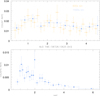 |
Fig. 1. X-ray data. Top: Chandra light curve of Cen in bins of 600 and 1500 s. Bottom: ACIS-S spectrum of Cen. |
3. Data analysis and results
3.1. Acquisition images and 2D frames
During the X-shooter data reduction process, inspection of the raw 2D frames revealed that the [O III]λ4959 showed emission line structures (blobs) that were tilted in some exposures (see Fig. 2, top). This effect is evident only in the [O III]λ4959 line since it is the strongest unsaturated line in the X-shooter UVB+VIS+NIR spectrum3. The presence of tilted emission structures suggests that the ejecta were possibly resolved. To check this hypothesis, we measured the point spread function (PSF) of Cen and five nearby stars in each acquisition frame (i.e., seven frames on night 1 and eight on night 2; Fig. 2, bottom). A Student t-test showed that Cen is somewhat larger than the average PSF in 47% of the frames. Hence, we conclude that the ejecta are marginally resolved. This would explain the occasional variation of the [O III] line profile observed in some spectra, especially on the second night. Possibly depending on the seeing variation and photon statistic, the centering of Cen in the slit might have been affected by bright structures in the ejecta (we used the Johnson V filter for the target acquisition, which at 5000 Å transmits almost 80% of the incoming light; see the instrument manual). Partial resolution of the ejecta may also explain the large uncertainties in the Gaia second data release (DR2) distance (317 pc, Bailer-Jones et al. 2018).
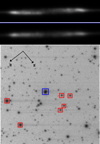 |
Fig. 2. Analysis of the X-shooter images. Top: examples of the [O III]λ4959 emission line as observed in the 2D raw frames. The bright spots correspond to the line structures (i.e., peaks) in the Fig. 3 profile. The wavelength increases from left to right. Bottom: X-shooter acquisition frame. The blue square encloses Cen, while the red ones cover the comparison stars that were used to estimate the seeing PSF. The field shown is 1.47 arcmin squared. |
We were able to use the resolved images to constrain the distance to Cen from its nebular parallax. Using the acquisition frames where the Cen PSF was resolved, we estimated the average size of the nebula to be ⟨FWHM⟩ = 0.44 ± 0.11 arcsec, where the individual values were calculated from  . The expansion velocity to adopt in the nebular parallax computation is not that observed during maximum or early decline, but rather that of the currently emitting ejecta. At the time of the X-shooter observations, the nebular emission lines were produced mainly by the inner ejecta because of the reduced emission measure of the highest velocity gas. Figure 3 shows that the strongest ejecta structures extend up to ∼800 km s−1 along the line of sight. For an ejecta inclination of 40 deg (Mason et al. 2018), this translates to an absolute maximum velocity of ∼1200 km s−1 and to a projected velocity on the sky plane of ∼950 km s−1. The latter produces a distance of about 2.4
 kpc, in agreement with our previous determination given the uncertainties (≃2 kpc, Mason et al. 2018).
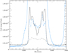 |
Fig. 3. [O III] λ4959 and Hβ line profiles in April 2019 (solid and dashed black lines, respectively), together with the same line profiles from March 2016 (blue lines) showing the change of the emission measure per velocity bin. The [O III] emission lines were about ten times stronger in 2016 than in 2019. |
3.2. The emission-line spectrum
Figure 4 shows the emission lines that dominate the Cen spectrum. We identified over 80 emission lines in the UVB+VIS+NIR spectrum of Cen. Of those, several have a purely ejecta origin, while the others are a varying mix of ejecta and binary contributions (see Appendix B). Pure ejecta lines were identified by their invariant profile, and they comprise forbidden transitions. Numerous permitted transitions also revealed, via their variable profiles, a contribution from the binary underneath. The observed variations are minimal but become obvious when trailed spectrograms are produced. The narrow s-wave in the transitions of the higher Balmer and Paschen H series, He I, and C IIλ4267 lines are clearly of a binary origin. Also of a binary origin are features we nicknamed “fuzzballs”, which appear almost in antiphase with the narrow s-wave. The fuzzballs are most visible in the higher Balmer, Paschen, and Brackett series lines and in the He I transitions. In addition, in the He I and in the NIR H lines, they morph into a complete sinusoidal curve (the “fuzzball-wave”). Figure 5 shows a selection of trailed spectrograms of nebular and permitted transitions. The visibility of the binary s-wave and fuzzballs in the H lines indicates that they have higher opacity and a flatter decrement than the ejecta (which satisfy case-B optically thin conditions). The presence of the fuzzball-wave in the H Paschen and Brackett lines where the s-wave disappears indicates that the gas producing the fuzzballs has a higher opacity than that producing the s-wave.
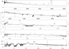 |
Fig. 4. Cen fiducial X-shooter spectrum. The UVB and VIS arm x-axes (top two panels) are in units of Å; NIR arm x-axes (bottom three panels) are in units of μm. The spectrum is not corrected for reddening. |
3.2.1. The radial velocity curve and the binary parameters
The contrast between the binary and the ejecta emissions is low and does not improve significantly after subtracting the ejecta template (e.g., from spectra of previous epochs or from a purely nebular emission line profile). Hence, the binary emissions cannot be fit or measured in individual spectra, but their positions and motions can be measured via a cursor position in the trailed spectrograms, especially for the s-wave. We did so for the s-wave in H I λ3797, 3835, 3889, and 3970, He I λ4026, 44714, 5876, 6678, and 7065, and C II λ4267. We also measured the fuzzball-wave for the He I λ6678 and 7065 trailed spectrograms.
We fit the Heliocentric radial velocity curve of each line separately, each ion (i.e., H I, He I, and C II) separately, and finally all measures together using
![Mathematical equation: $$ \begin{aligned} { v}_r=\gamma +K\times \sin {[(t-t_0)/P]}, \end{aligned} $$](/articles/aa/full_html/2021/05/aa40050-20/aa40050-20-eq4.gif) (1)
(1)
where γ is the systemic velocity, K is the amplitude of the s-wave and can be negative, P is the period, and t is the mid MJD of each exposure. We chose the time of the first red-to-blue crossing on each night for t0. The best fit parameters, γ, K, and P, and their associated errors were determined through a bootstrapping technique (e.g., Wall & Jenkins 2012). Before combining the radial velocity measures from different transitions, we always checked that the χ2 distribution of the individual fits were comparable. We also overplotted the measures from a given line on the trailed spectrogram of other transitions to visually check the consistency. Table 1 gives the best fit for the s-wave parameters obtained by combining all the H I, He I, and C II measurements for each night. It also gives the best fit obtained for individual atomic species or ions. Figure 6 shows the H and He I radial velocity measures together with the global best fit sine functions from night 1.
S-wave radial velocity fits.
The sets of parameters are fairly similar between the two nights. The time elapsed between the s-wave curve of the two nights is 12.995 ± 0.002 days (i.e., shifting night 1 by 12.995 days, its data points superpose well with those of night 2), which corresponds to ∼82.7 or 84.5 cycles for the periods of night 1 and night 2, respectively. Taking all the uncertainties into account, P = (12.995 ± 0.002)/N with 82 ≤ N ≤ 85 or 0.152859 ≤ P ≤ 0.158500 days (i.e., 3.67 ≤ P ≤ 3.80 h). This agrees with the periods and uncertainties in Table 1. For the reminder of the paper, we adopt the orbital period corresponding to exactly 83 cycles as the system’s orbital period: P = 12.995/83 days∼3.76 h.
We ascribe the narrow s-wave emission to regions near the L1 point on the secondary star. This assignment is supported by its regular pattern, its reduced visibility when it moves from maximum blueshift to maximum redshift, and its velocity width.
Looking at Table 1, while it seems reasonable and statistically correct to combine the various transitions from different species to produce a single best fit per night, we note that the best fit for each ion separately produces larger K values for He I lines than for H lines, which, again, have a greater K than C II 4267. This arises from two observational biases. First, not all s-waves are complete, and they are generally weaker in the branch from maximum blueshift to maximum redshift. Second, the s-wave width is not the same for all ions, especially at the velocity extremes. This suggests that the bulk of emission of a given transition is sited differently around the L1 point, perhaps occupying different fractional areas of the substellar hemisphere. Similarly, the systemic γ velocity depends on the ion, γ(HI) > γ(CII) > γ(HeI), and is possibly the result of a velocity gradient in the secondary star “chromosphere”.
The identification of the mean location of the s-wave with the L1 point, together with its radial velocity curve and the period, provides a mean for deriving the binary system parameters: mass ratio, secondary star mass (for an assumed WD mass), and separation. From the relation valid for the center of mass, a1M1 = a2M2, and the definition a = a1 + a2, where M1 and M2 are the primary WD and the secondary donor star mass, a1 and a2 are the distance of each star from the binary center of mass, and a is their separation:
 (2)
(2)
with P being the orbital period and RRL(2) the Roche lobe radius of the secondary star, for which we use the Eggleton (1983) approximation:
 (3)
(3)
If the orbital inclination of the binary is the same as that of the ejecta, i ≈ 40deg, K2 ≈ 270 km s−1, and for a WD mass M1 = 1.2 M⊙ (José et al. 2020), we obtain q ≳ 0.17 and a secondary mass M2 ≈ 0.21 M⊙. Alternatively, we can use the orbital period and the P − M2 and P − R2 empirical relations in Knigge et al. (2011) to constrain the secondary star mass and radius. We find R2 ≈ 0.36 R⊙ and M2 ≈ 0.29 M⊙. Consistent results (R2 ≈ 0.39 R⊙ and M2 ≈ 0.34 M⊙) are found by adopting the Howell et al. (2001) theoretical relations. Hence, for M1 = MWD = 1.2 M⊙, 0.24 ≤ q ≤ 0.28 and a ≈ 1.4 R⊙. For the derived parameters, the secondary star roughly matches an M3.5V-M4.5V spectral type (Torres et al. 2010). These are the spectral types we employ in the analysis in Sect. 3.3.1.
3.2.2. The fuzzballs and the multi-emission simulation
The trailed spectrograms of the VIS arm He I transitions suggest that the fuzzballs are not a confined emission region that appears only at unique orbital phases, but a source that is always visible during its orbital motion around the binary center of mass. This is even more evident in the trailed spectrograms of the H Paschen and Brackett series (see Fig. 5). The superposition of the emission from the fuzzball-wave with the that from the ejecta simply makes it more visible at maximum blueshift and redshift in the bluer H-Balmer transitions. Measuring the fuzzball-wave of the VIS arm He I lines5 and fitting their radial velocity using bootstrapping techniques as we did for the L1 s-wave, we obtained the radial velocity parameters given in Table 2 and Fig. 6. The fuzzball-wave is not exactly in antiphase with the L1 s-wave. So although it arises from a region within the WD Roche lobe, it is not symmetrically distributed around the WD and cannot trace the WD orbital motion. The exact phase difference is ϕRB(s-wave)−ϕRB(fuzzball-wave) ≃ 0.58 periods, meaning that the fuzzball-wave extremes (i.e., max blue- and redshifts) anticipate those of the L1 s-wave by ∼0.08 orbital periods. Within the standard convention where phase 0 is the secondary inferior conjunction6, the secondary star L1 emission reaches maximum blueshift (redshift) at phase 0.75 (0.25), as expected. The fuzzball region, instead, reaches maximum blueshift (redshift) at phases 0.18 (0.68). Red-to-blue crossing occurs at phase ∼0.93. The phase shift suggests that the fuzzball-emitting region could arise from the stream impact point and that we see maximum redshift (blueshift) when we look upstream (downstream).
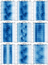 |
Fig. 5. Selected trailed spectrograms from night 1. Darker regions indicate stronger emission (linear intensity scale). From top to bottom and left to right: Hη, Hζ, C II λ4266, He II λ4686, He Iλ7065, He II λ10123, [Ar III] λ7135, H Paschen λ8862, and H Brackett λ15880. The y-axis in each panel indicates the spectrum number in the night time series. The fuzzballs are particularly evident at maximum blueshift around spectra 10 and 30, as well as at maximum redshift around spectra ∼20 and 40 in the Hη, Hζ, He Iλ7065, and H Paschen λ8862 lines. |
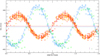 |
Fig. 6. Radial velocities of the s-wave (red and orange diamonds for night 1 and night 2, respectively) and of the fuzzball-wave (blue and green squares for night 1 and night 2, respectively). The red sine curve and horizontal lines are the night 1 best fit radial and γ velocity for the s-wave, respectively (see Sect. 3.2.1 for details). The blue sine curve and horizontal line are the night 1 best fit radial and γ velocity, respectively, for the fuzzball emission (see Sect. 3.2.2 for details). The two vertical bars on the bottom right corner of the panel represent the radial velocity measurement 1σ uncertainties: 30 km s−1 in purple for the UVB arm measurements and 20 km s−1 in dark green for the VIS arm measurements. |
Fuzzball-wave radial velocity fits.
Figure 7 shows a simulation produced by superposing a nebular line profile with a narrow (∼50 km s−1) Gaussian emission and a broader (∼300 km s−1) boxy emission with the phase offset mentioned above and with a velocity amplitude matching the best fit K of the s-wave and fuzzball-wave, respectively. The simulation qualitatively reproduces our observations, supporting the contention that the fuzzballs arise from an emitting region within the WD Roche lobe that is continuously visible around the orbit. We did not obtain significant differences when replacing the boxy profile with a different one (e.g., a disk or double-peaked profile). Thus, although we cannot definitively constrain the geometry or the ultimate nature of the emitting region, the fuzzballs’ source cannot match an accretion disk because of its asymmetric location, phasing, and K value. Instead, it can match a stream impact region within the circum-WD matter.
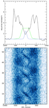 |
Fig. 7. Simulation of the emission line components. Top: Cen nebular line ([Ar III]λ7135, black line), together with the Gaussian (blue) and the “boxy” (green) profiles used in our simulation. Bottom: simulated trailed spectrum. See Sect. 3.2.2 for details. |
Since we are not aware of any cataclysmic variable (CV) with an optically thin hotspot (intended as the classic stream-disk impact point) and an optically thick disk (e.g., Warner 1995; see also Sect. 4), we further checked for possible accretion disk signatures in the emission line wings. Specifically, we inspected the trailed spectrogram after enhancing the contrast at the wing level and searched for any coherent motion using the bisector technique for the wings of isolated and relatively strong emission lines, such as Hβ, Hε, and He II (and [OIII] for consistency). We found values randomly scattered within ≲40 km s−1. The expected WD orbital velocity amplitude for the system parameters in Sect. 3.2.1 is ∼60 km s−1, that is, the probed quantity would be at the limit of our precision.
We also note that the emission lines have FWZI ∼ 1300 km s−1 (where FWZI is the full width zero intensity), implying that they cannot probe any region close to a WD at its expected equilibrium radius, such as the inner accretion disk. This also excludes high velocity wings of the isolated single-peaked emission lines that are observed in some SW Sex type stars (e.g., Rodriguez-Gil et al. 2007).
3.3. The continuum spectrum
Since for most of the night the Cen observations were obtained at a better seeing than the spectrophotometric standard star EG 274, the Cen spectra tend to be overestimated in the blue flux. Selecting the spectra that have UVB and VIS PSFs roughly matching those of EG 274, we can be confident that their SED is accurate. However, the Cen spectra that have PSFs that match or are comparable to those of the spectrophotometric standard in the UVB and VIS arm might have non-matching PSFs in the NIR arm. This is because, in addition to the optics and the seeing, the NIR PSF also depends on sky conditions, such as the humidity and the number and sizes of aerosols. Thus, we chose spectrum 4 for night 1 and spectra 8 and 42 for night 2 as fiducial reference spectra for inferences about the Cen SED (Sect. 3.3.1) and its long-term evolution (Sect. 3.3.4) since they were obtained at a seeing comparable to that of the spectrophotometric standard. The spectra, although from different nights and at slightly different orbital phases, are consistent with the same SED. Their ratios are constant, and they differ in flux by ∼6%, 5%, and 13%, in the UVB, VIS, and NIR arms, respectively.
3.3.1. The SED and its components
Figure 8 shows the Cen SED after correction for interstellar reddening, E(B − V) = 0.15 mag (Mason et al. 2018). The top panel zooms in on the two X-shooter fiducial spectra, while the bottom panel shows the complete data set from the x-ray to the NIR wavelengths. We compared the data with a number of stellar photosphere models and an arbitrarily scaled power law that would be expected for an optically thick accretion disk in steady state (e.g., Pringle 1981). We selected stellar models that most closely matched the two stars composing the binary system. For the donor star we chose a 3100 K, log g = 5 or 4.5 solar abundance model (red lines in the figure) from the Next Generation database (Allard et al. 1997; Hauschildt et al. 1999 and references therein), which is consistent with our results in Sect. 3.2.1 and the Torres et al. (2010) calibrations. For the primary we selected models from the Koester WD database (Koester 2010; Tremblay & Bergeron 2009) and the Tubingen non-local thermodynamic equilibrium (NLTE) model atmosphere database (Rauch et al. 2018). The Tubingen models are He-rich (50% by number). The temperature was limited to the range 40 000–50 000 K, based on the observed s-wave transitions and assuming that the L1 region is excited by the WD. Since we detected only H, He I, and C II transitions and not He II or Ca II, the bulk of the source radiation must be confined within 10 and 50 eV, that is, consistent with a Teff ≤ 50 000 K photosphere. We set log g to 8.25, as appropriate for a ∼1.2 M⊙ WD (as shown by the lines of various blue shades). Both the donor and the WD models have been scaled to the distance of 2 kpc.
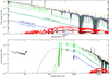 |
Fig. 8. Cen continuum SED and comparison with theoretical models. Top panel: Cen fiducial reference spectrum 4 from night 1 (solid black line) and the fiducial spectrum 8 from night 2 (dotted gray line). Both have been corrected for reddening. The solid orange line represents a power law of power −7/3, as predicted for steady state accretion disks; all the other colored lines are stellar atmosphere models. Their temperatures and gravities are marked in the figure itself (shade of blues for the Koester WD models; shades of green for the Tubingen database stellar atmospheres; shades of red for the Next Generation NLTE cool stars models). Bottom panel: fiducial reference spectrum 4 from night 1 together with the Swift UVOT photometry (filled black circle for the April 2019 observation; open magenta squares for the June 2019 observations), the Chandra spectrum, the same models as in the top panel, and a T = 50 kK log g = 7.0 model with solar abundances (magenta line; Tubingen database). |
It is immediately clear why we detect no signatures from the secondary star: Its fractional contribution is at most a few percent of the total observed flux. For the same reasons, a normal WD cannot be detected, even at UV wavelengths. Both the WD and the donor are outshone by something else. It is also evident that the SED slope does not quite match the steady state accretion disk slope. It is not rare for a CV SED to deviate from that of an optically thick accretion disk (see Sect. 4), although best matches are found, and expected, for disks with high mass transfer rates (e.g., SS Cyg during outburst; Kiplinger 1979; see also Warner 1995). Linear fits to the Swift photometry and points on the optical+NIR continuum show that the Cen SED is better represented by a broken power law with power −2.4 in the near-UV (NUV) range (in good agreement with the optically thick steady state accretion disk) and a steeper slope (power −3.2) longward of ∼4000 Å.
We can proceed by making two different alternative hypotheses: (1) The dominant emitting source is the accretion disk, both in the optical and the NUV. (2) A bloated WD photosphere is the major continuum source in this wavelength range.
For hypothesis 1, we can compute the NUV+optical+NIR luminosity and use it to constrain the accretion disk mass transfer rate. The de-reddened flux of the least overlapping Swift UVOT filters is Fuvw2 + uvw1 = 2.4 × 10⁻¹⁰ ± 1.1 × 10⁻¹³ erg cm−2 s−1, and the average integrated flux of the de-reddened fiducial spectra after removal of the emission lines is FUVB + VIS + NIR = 2.2 × 10⁻¹⁰ ± 4.8 × 10⁻¹² erg cm−2 s−1. This gives a luminosity LNUV − NIR = 1.8 × 1035 erg s−1 ≃ 47 L⊙. Then, approximating Ṁ ∼ 2LRWD/(GMWD), with the usual meaning of the symbols, and adopting MWD = 1.2 M⊙ (hence RWD ≃ 0.0115 R⊙), we get the mass accretion lower limit, log(M⊙ yr−1) ∼ − 7.5, which is larger than what is typical for CVs above the period gap (Howell et al. 2001; Knigge et al. 2011) or measured in old nova systems7 (Selvelli & Gilmozzi 2019). It must be noted that this is a conservative lower limit since we do not have a measure of the far-UV (FUV) flux where most of the accretion disk luminosity is expected to emerge. Using the above power-law fit to the Swift photometry and extending it to the International Ultraviolet Explorer (IUE) range (1250–3050 Å), we can estimate the Cen UV luminosity and compare it to that (uncorrected for geometrical effects) of the old novae in Selvelli & Gilmozzi (2019). We find LIUE ∼ 63 L⊙, which is larger than the values in Table 2 of Selvelli and Gilmozzi, as we will discuss in Sect. 4.
For hypothesis 2, we can check the lowest log g that is compatible with the data. Figure 8 shows that the He-rich photosphere model of T = 50 000 K and log g = 5.7 (lime line) can match our data and the Swift NUV photometry as well as the power-law approximation of the optically thick accretion disk. Models of intermediate log g between this upper limit and that appropriate for an equilibrium WD are also plotted for comparison. The bloated WD photosphere with log g = 5.7 would be as large as ≤0.25 R⊙ (i.e., almost ∼20 times a normal WD radius) and ∼0.3 RRL(WD). As unconventional as this may appear, it is an alternative to the almost Roche lobe filling accretion disks proposed for similarly bright systems (e.g., HR Del; Bruch 1982). In addition, the NUV slope, so similar to that of a stellar photosphere model, together with the flatter optical+NIR continuum, is consistent with an expanded WD envelope whose cooler outer layers are more opaque than the inner ones and are responsible for a flatter optical slope. Any possible absorption lines from such an expanded WD envelope, if present, are masked by the emission lines from the rest of the binary and the ejecta.
3.3.2. The WD accretion rate from the x-ray data
The Chandra spatial resolution is poorer than the estimated nebula size in the optical, and therefore it does not resolve the ejecta. Nevertheless, the x-ray signal detected with Chandra certainly originates in the binary and not from the ejecta. Only a few novae, several decades to a century old, have shown x-ray emission due to the interaction between the interstellar medium and the ejecta (e.g., Takei et al. 2013 and reference therein). Cen is not located in a particularly dense interstellar region, and it is still too soon after its eruption to have accumulated enough ambient material to be detectable in the x-rays.
Cen has an integrated flux of FX ≃ 2.2 × 10⁻¹³ erg s−1 in the range 7–12.4 Å (about 1.0–1.8 keV), corresponding to the luminosity LX = 1 × 1032 erg s−1 for the adopted distance of 2 kpc. Although a direct comparison with published x-ray and optical observations of other bright CVs is not straightforward, because of the slightly different energy and wavelength ranges, we note that the derived luminosity is in line with that derived for other CV and nova-like (NL) systems (e.g., Balman 2020 and reference therein), and the ratio between the x-ray and the optical flux is consistent with that observed in high mass transfer rate systems (e.g., Kuulkers et al. 2006 and references therein).
Where the x-ray originates in the system cannot be definitively assigned at this stage. Considering the error bars and the low source counts, the x-ray signal is consistent with no modulation over the orbital period, indicating that the emitting region is always in view. It could originate in the WD boundary layer, which yields an estimated mass accretion rate of log(M⊙ yr−1)X ∼ −10.8, that is, almost three orders of magnitude smaller than that derived from the optical SED. Alternatively, it could arise from any of the additional regions hypothesized to explain the x-ray optical flux dichotomy (Kuulkers et al. 2006 and reference therein; see also Mukai 2017 and Balman 2020). However, such a low x-ray emission could originate at an impact site within the WD Roche lobe, with the accretion onto the WD being extremely inefficient and therefore remaining undetected.
3.3.3. Short-term SED variations: Within and across nights
In the attempt to construct a continuum light curve from the spectra, we first tried to mitigate the color effects induced by the seeing and the flux calibration (see the beginning of Sect. 3.3). We determined the wavelength dependence of the spatial PSF (each X-shooter arm is a separate cross-dispersed echelle spectrogram) by measuring the width of the spectrum at three points along each separate order. We then fit a quadratic function after normalization to a selected wavelength in each arm and used the fit to roughly correct for slit losses. Such a correction is appropriate for relative comparisons of the continuum flux within an arm. It is not a method for absolute flux calibration or SED reconstruction.
The differential photometry was extracted from portions (10 to 60 Å wide) of the continuum and then compared, for consistency, with the integrated flux of nebular lines, keeping in mind that the continuum source and the nebular lines are not necessarily co-spatial (see Sect. 3.1). We found similar light curve patterns in the continuum and the nebular lines and thus conclude that the source flux is constant to within the precision of our method (∼15, 25, and 20 percent in the UVB, VIS, and NIR arm, respectively). The lack of any intrinsic variability in the K band is particularly interesting since it supports our results from Sect. 3.3.1, indicating that tidal distortion of the secondary star is outshone by a stronger light source, and that a high energy radiation incident on the WD-facing side of the donor does not penetrate deep into the stellar photosphere, affecting only its upper layer.
3.3.4. SED long-term evolution: From late nebular to today
The comparison of our fiducial reference spectra with those from previous epochs provides information about the evolution of the SED. Figure 9 displays the optical part of the fiducial reference, spectrum 4, on night 1 together with the VLT/UVES spectra taken at ∼1.3, 1.6, and 2.3 years after the nova outburst.
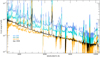 |
Fig. 9. Comparison of the UVES spectra with our fiducial spectrum from night 1. We note that since UVES spectra do not extend into the NIR wavelengths, the X-shooter NIR spectrum is not shown. The spectra have been corrected for interstellar reddening. |
The absolute flux calibration of the UVES spectra is not sufficiently accurate and the blue part of the spectra is likely underestimated since the flux calibration was performed with the observatory standard star, which is observed with a much wider slit than Cen. We verified, using passbands described in Bessel (1976), that the derived synthetic photometry was usually consistent with the American Association of Variable Stars Observers (AAVSO) pre-validated V band photometry but significantly fainter than the B band photometry at the same epochs. Differences as large as 1.4–1.5 mag point to systematics that can be significant, especially for the B band (Munari & Moretti 2012). In addition, the AAVSO photometry can vary among observers, and it typically came from only one observer per epoch. Consequently, we did not adjust the UVES data to the AAVSO photometry. Nevertheless, the UVES spectra are similar to one another and different from that detected with X-shooter in the more pronounced continuum excess below ∼4000 Å, and possibly below ∼8500 Å. This suggests stronger continuum radiation from recombination (mainly H–I free-bound transitions) from the ejecta at the time of the UVES observations. However, the X-shooter spectrum suggests that some recombination continua also come from the binary system and the ongoing accretion. To better understand the relative contribution of the ejecta and the binary, we measured the continuum flux at different portions of the spectrum along with the integrated flux of a few emission lines. Figure 10 shows how the continuum and emission line fluxes decrease. It is evident that the forbidden transitions decline roughly as a power law in time, consistent with forming in an environment of decreasing density and in the absence of any new photoionizing source (Shore et al. 2016). In contrast, the continuum flux and the He II transition flatten out, indicating that a new source is contributing (in addition to recombination from the ejecta).
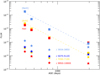 |
Fig. 10. Flux decline rate from day 489 to 1958 as measured in a portion of the continuum (star symbols) as well as in selected emission lines (square symbols): two nebular lines ([Ne III]λ3869 and [Ar III]λ7135) and a permitted one (He II λ10124). |
4. Discussion and conclusions
Cen is a typical CN. Only because of its brightness was it so extensively observed from maximum to late decline up to 5.4 years after the outburst. What makes this nova special is the collected data set that is not available for other systems: multi-epoch UV and optical high resolution spectroscopy from early decline to late nebular stages, Swift x-ray monitoring during the whole outburst, and, now, medium resolution time-resolved optical+NIR spectroscopy complemented with Swift and Chandra observations. The collected observational evidence should, therefore, be representative of any CN of intermediate speed class and inclination.
Observationally, we identify two sinusoidal patterns that vary in antiphase. One is a narrow sine wave with velocity amplitude ∼178 km s−1 (the s-wave). It is fairly narrow and has varying visibility, being more evident during the red-to-blue branch of the radial velocity curve. This phenomenology suggests that it can be assigned to the irradiated face of the secondary star. In particular, since the line width is narrow, the emitting region is fairly small – that is, not extended over the whole hemisphere facing the WD – and is probably confined to the proximity of L1. We rule out the possibility that the narrow s-wave is from the stream (other than possibly the very initial part near L1) because the emission line width would be greater (due to the velocity gradient) and would have a different visibility pattern. More importantly, the stream has too low a density – and therefore a negligible emission measure – to be the dominating source.
Irradiation of the secondary star is observed in CVs (e.g., Catalán et al. 1999, Harrison et al. 2003, Southworth et al. 2008, Schmidtobreick et al. 2018), and it is expected in novae for which an increased mass transfer rate is predicted as a consequence of the expected high WD temperature (Shara et al. 1986; Kovetz et al. 1988). We note, however, that the observed irradiation is not quite as modeled by Barman et al. (2004; and specifically for the CV VV Pup in Mason et al. 2008). Cen displays only emission lines, while the continuum remains unaffected by the incident radiation; the incident high energy flux on the donor does not penetrate deep into the stellar photosphere and only produces a chromosphere-like emission in its upper layer. The temperature inversion caused by the irradiation is, however, different from a typical chromosphere since we detect transitions from higher ionization potential energy ions than in typical stellar chromospheres, namely H, He I, and C II without Na I D and Ca II. The detected species constrain the ionizing source energy distribution. In particular, the lack of singly or doubly ionized metal lines and He II suggests an irradiating source close to ∼50 000 K in color temperature. We propose that the irradiating source is the WD, which is, however, much more extended than expected from the equilibrium mass-radius relation. From this s-wave we derive the system orbital period and, with a few assumptions, system parameters such as the secondary star mass and radius and the mass ratio (see Sect. 3.2.1).
The second sinusoidal pattern is the one we nicknamed fuzzballs because of its very localized visibility in the upper H Balmer series lines. However, its periodic visibility is simply due to the superposition of different contributions: the fuzzball source and the ejecta. As already mentioned, the fuzzballs morph into a complete sinusoidal pattern in the Paschen and Brackett series. The amplitude and phase of the fuzzball-wave match the position of an impact region well. The region appears to be optically thin gas because its emission is not modulated with orbital phase.
In the conventionally adopted picture of CVs (Warner 1995 and references therein), the systems with low mass transfer rates host (at least partially) an optically thin disk that generates emission lines together with a stream-disk impact region (the hotspot). Instead, high mass transfer rate systems tend to have optically thick disks with absorption lines and, occasionally, superposed weak to no emissions. In these systems any hotspot contribution is overwhelmed by the continuum emission from the disk. If we interpret the fuzzball-wave as the hotspot, we face an anomaly since we see emission lines from the impact region but not from the disk. However, SW Sex stars are similarly anomalous systems with only a single-peaked emission producing a relatively large velocity amplitude sinusoidal wave (on the order of a few hundred km/s), and with occasional evidence for an irradiated face of the secondary star. The identifying characteristics of the class (Rodriguez-Gil et al. 2007) are the maximum blueshift of the sinusoidal wave at orbital phase 0.5, transient absorption features at about the same orbital phase, high velocity wings (even up to a few thousand km/s) whose radial velocity curve is offset in phase (by 0.1–0.2) with respect to that of the bulk of the emission, and, as noted by Dhillon et al. (2013), flux variation of the emission lines that drives the broadband photometry variability. SW Sex stars do not necessarily fulfill all these conditions simultaneously (even the prototype itself happens to lack many; Dhillon et al. 2013 and reference therein), but Cen has none of them. The anomaly extends to the continuum emission. Although multiband studies of bright CV SEDs are not numerous, Kiplinger (1979) has shown that the SED of the SS Cyg accretion disk during outburst matches the theoretically predicted SED of an optically thick, geometrically thin accretion disk from the FUV to the mid-IR. Similarly, Ciardi et al. (1998) found that the accretion disk of the NL V592 Cas matches a power-law distribution with power −2.3 from the U to the NIR, in excellent agreement with the Pringle (1981) approximation. In contrast, Hoard & Szkody (1997) report a flat optical continuum (in wavelength) for the SW Sex stars.
The SED analyses of the accretion disk in bright CVs have been generally limited to the UV wavelength because this is where most of the accretion disk flux is emitted. Puebla et al. (2007), analyzing UV spectra (IUE and Hubble Space Telescope, HST) of NL systems and old novae (i.e., systems supposedly hosting a stable accretion disk), found that that optically thick, geometrically thin Keplerian disk models cannot fully reproduce the observations; the authors suggest a number of scenarios that can be explored to improve the fitting and remove degeneracy. Selvelli & Gilmozzi (2013) used IUE, Far Ultraviolet Spectroscopic Explored (FUSE), and HST/STIS spectra of old novae, fitting them with a power law. They found a different power for each nova, ranging from −0.32 to −2.55 or −0.35 to −2.88, depending on the adopted reddening law. Gilmozzi & Selvelli (in prep.) found a similar range of powers (−0.15 to −2.36) analyzing the IUE spectra of NL systems (including SW Sex systems). Selvelli & Gilmozzi (2019) and Gilmozzi & Selvelli (in prep.) also computed the IUE luminosity for each object using the Gaia releases. Even if the Cen UV slope is consistent with that of an optically thick accretion disk and in the range observed for old novae and NL systems, the difference between Cen and NL systems or old novae becomes more obvious when the fluxes are converted to luminosity. The average luminosity of NL systems is ∼3 ± 2 L⊙ and that of old novae is larger and more scattered, ∼6 ± 7 L⊙, depending on the age of the old nova (17–29 to 132–147 yr after outburst). Both results exclude the anomalously bright objects QU Car (for the NL systems) and HR Del (for the old novae), whose luminosities (40 and 64 L⊙, respectively) are much closer to the 63 L⊙ estimated for Cen in Sect. 3.3.1. The reasons to treat those objects separately are the debated nature of QU Car and the relatively young age of HR Del at the time of the IUE observations (12–25 yr). It has been suggested that QU Car belongs to the V Sge star class (Oliveira et al. 2014) and is one of those permanent super soft source binaries that miss detection in the x-ray because of high interstellar extinction. HR Del was an extremely slow nova with an anomalous light curve that could result from unstable burning, as proposed for the recent transient ASASSN-17hx (Mason et al. 2020), and with a similarly extremely large ejecta mass (9 × 10⁻⁴ M⊙; Moraes & Diaz 2009). In other words, both objects are neither typical nor representative of their own class, and both could have ongoing burning and, therefore, a completely different WD structure.
The classic default assumption of a fully reformed stationary accretion disk might not be the most appropriate when confronting a system that only ∼5 years ago experienced a nova outburst, has an extraordinary luminosity, and is still over 1 mag brighter than before the outburst. We need to determine if the assumption of such a disk is realistic. The WD has experienced a thermonuclear runaway (TNR), and it is still unknown whether a disk can survive the blast. Similarly uncertain is how the WD relaxes and on what timescales. It is hard to imagine that the primary Roche lobe is empty except for the WD after the TNR. Any (He) envelope remaining on the WD surface (e.g., Prialnik 1986; Newsham et al. 2014) should relax on thermal timescales once all nuclear burning has ceased8. But even whether that stage has been reached so soon is theoretically uncertain. Unfortunately, observations cannot probe the system status during the optically thick phase of the outburst (which depends on the wavelength). Additionally, theoretical models and simulations have, to date, focused on different issues, such as the TNR nucleosynthesis, the mixing, the ejecta mass, and the ultimate growth of the WD to the Chandrasekhar limit (e.g., Starrfield et al. 2016; José 2016; Yaron et al. 2005; Hillman et al. 2016), and, because of computing time limitations, they are one-dimensional. Last but not least, smooth particle hydrodynamic simulations of accretion disks use idealized initial conditions, for example, an empty Roche lobe (Frank et al. 2002 and references therein).
Instead, adopting an unusual but not unprecedented scenario of a still expanded WD envelope surrounded by gas (from the TNR leftover and from the secondary), we can consistently explain our observations. The expanded WD photosphere scenario was first proposed by Shore et al. (1997) for the ONe nova V1974 Cyg. There, UV spectra taken ∼3 yr after outburst showed that the Lyα absorption from the primary and the continuum were better matched by a log g = 6 photosphere than by the log g = 8 one. While the estimated luminosity was larger than theoretically predicted for a relaxed WD, it was consistent with the derived continuum for an effective temperature of 20 000 K.
For Cen, the bloated WD envelope can account for most of the system luminosity, the exact fraction depending on the chosen log g. The unsettled gas within the WD Roche lobe, while not excluding density concentrations on the orbital plane, explains the lack of accretion disk signatures since bound material in chaotic motion emits all over the place in any given transition. Finally, the fuzzball-wave, being self-similar at any phase, can be explained with the stream impacting optically thin low-density gas without developing any gradient or wake at the impact point.
The proposed scenario is quite different from those for U Sco, LMC 1968, and nova Her 1991, for which evidence of early accretion disk formation has been reported. While the data sets are not directly comparable, these are either recurrent nova systems or extremely fast CNe for which the ejecta masses are orders of magnitude smaller than those of Cen and the super soft source phases are much shorter.
The [O III]λ5007 emission line is saturated in all the exposures except the shortest. The [N II]+Hα blend is present in order 25 and order 24 of the VIS arm. It is saturated in order 25 and much weaker in order 24.
This line, however, seems to be biased by a blending emission.
We did not measure the radial velocity of the H Paschen or Brackett transitions because of their width and low S/N (especially when telluric absorptions or poorly removed sky emission lines are superposed).
The t0 defined in the previous section corresponds to phase 0.5 in this convention.
A direct comparison, however, is not possible since Selvelli and Gilmozzi computed the Ṁ over a different wavelength range and taking inclination and limb darkening effects into account.
The accumulated mass before the outburst is in the range 10−5–10−4 M⊙, but the ejection efficiency is highly uncertain and debated. The other free parameters in the computation of the thermal timescale (WD mass and radius) are similarly uncertain. An estimate for the WD radius, in particular, would require dynamically simulating the WD structural evolution from the time of the ejection through its relaxation to equilibrium. Such models are currently unavailable. Nevertheless, depending on the assumed parameters, estimates of the thermal timescale vary from years to a century. For Cen, assuming that at least ∼3% of the accreted envelope remained on the WD surface (Prialnik 1986), the thermal timescale is ∼4–5 years at the observed luminosity and for WD radii as large as 0.2–0.25 R⊙. However, both the WD luminosity and radius are a decreasing function of time.
Acknowledgments
EM thanks Yazan Al Momany for unveiling SM secrets. The authors also thank Jordi José and Juan Echevarria for discussion and Pierlugi Selvelli both for discussion and for sharing unpublished results. We are very grateful to the referee, John Thorstensen, for having provided constructive feedback that greatly improved our work.
References
- Allard, F., Hauschildt, P. H., Alexander, D. R., et al. 1997, ARA&A, 35, 137 [NASA ADS] [CrossRef] [Google Scholar]
- Bailer-Jones, C. A. L., Rybizki, J., Fouesneau, M., Mantelet, G., & Andrae, R. 2018, AJ, 156, 58 [NASA ADS] [CrossRef] [Google Scholar]
- Balman, S. 2020, AdSpR, 66, 1097 [Google Scholar]
- Barman, T. S., Hauschildt, P. H., & Allard, F. 2004, ApJ, 614, 338 [NASA ADS] [CrossRef] [Google Scholar]
- Bessel, M. S. 1976, PASP, 88, 557 [NASA ADS] [CrossRef] [Google Scholar]
- Breeveld, A. A., Landsman, W., Holland, S. T., et al. 2011, AIPC, 1358, 373 [Google Scholar]
- Bruch, A. 1982, PASP, 94, 916 [NASA ADS] [CrossRef] [Google Scholar]
- Ciardi, D. R., Howell, S. B., Hauschildt, P. H., et al. 1998, ApJ, 504, 450 [NASA ADS] [CrossRef] [Google Scholar]
- Catalán, M. S., Schwope, A. D., & Smith, R. C. 1999, MNRAS, 310, 123 [Google Scholar]
- Dhillon, V. S., Smith, D. A., & Marsh, T. R. 2013, MNRAS, 428, 3559 [NASA ADS] [CrossRef] [Google Scholar]
- Eggleton, P. P. 1983, ApJ, 268, 368 [NASA ADS] [CrossRef] [Google Scholar]
- Frank, J., King, A., & Raine, D. 2002, in Accretion Power in Astrophysics (Cambridge University Press) [Google Scholar]
- Fuentes-Morales, I., Tappert, C., Zorotovic, M., et al. 2021, MNRAS, 501, 6083 [Google Scholar]
- Hanuschik, R., & Amico, P. 2000, Msngr., 99, 6 [Google Scholar]
- Harrison, T. E., Howell, S. B., Huber, M. E., et al. 2003, ApJ, 125, 2609 [Google Scholar]
- Hauschildt, P. H., Allard, F., & Baron, E. 1999, ApJ, 512, 377 [NASA ADS] [CrossRef] [Google Scholar]
- Hillman, Y., Prialnik, D., Kovetz, A., et al. 2016, ApJ, 819, 168 [NASA ADS] [CrossRef] [Google Scholar]
- Hoard, D. W., & Szkody, P. 1997, ApJ, 481, 433 [NASA ADS] [CrossRef] [Google Scholar]
- Howell, S. B., Nelson, L. A., & Rappaport, S. 2001, ApJ, 550, 897 [NASA ADS] [CrossRef] [Google Scholar]
- José, J. 2016, in Stellar Explosions - Hydrodynamics and Nucleosynthesis (Boca Raton: CRC Press) [Google Scholar]
- José, J., Shore, S. N., & Casanova, J. 2020, A&A, 634, A5 [EDP Sciences] [Google Scholar]
- Kiplinger, A. L. 1979, ApJ, 234, 997 [NASA ADS] [CrossRef] [Google Scholar]
- Knigge, C., Baraffe, I., & Patterson, J. 2011, ApJS, 194, 28 [NASA ADS] [CrossRef] [Google Scholar]
- Koester, D. 2010, MmSAI, 81, 921 [Google Scholar]
- Kovetz, A., Prialnik, D., & Shara, M. M. 1988, ApJ, 325, 828 [NASA ADS] [CrossRef] [Google Scholar]
- Kuin, N. P. M., Page, K. L., Mróz, P., et al. 2020, MNRAS, 491, 655 [Google Scholar]
- Kuulkers, E., Norton, A., Schwope, A., et al. 2006, in Compact Stellar X-Ray Sources, eds. W. H. G. Lewin, & M. van der Klis (Cambridge University Press) [Google Scholar]
- Leibowitz, E. M. 1993, ApJ, 411, 29 [Google Scholar]
- Leibowitz, E. M., Mendelson, H., Mashal, E., et al. 1992, ApJ, 385, 49 [NASA ADS] [CrossRef] [Google Scholar]
- Modigliani, A., Goldoni, P., Royer, F., et al. 2010, SPIE, 7737E, 28 [Google Scholar]
- Mason, E., Howell, S. B., Barman, T. S., et al. 2008, A&A, 490, 279 [NASA ADS] [CrossRef] [EDP Sciences] [Google Scholar]
- Mason, E., Shore, S. N., De Gennaro Aquino, I., et al. 2018, ApJ, 853, 27 [NASA ADS] [CrossRef] [Google Scholar]
- Mason, E., Shore, S. N., Kuin, N. P. M., et al. 2020, A&A, 635, A115 [EDP Sciences] [Google Scholar]
- Moraes, M., & Diaz, M. 2009, ApJ, 138, 1541 [Google Scholar]
- Mukai, K. 2017, PASP, 129, 062001 [Google Scholar]
- Munari, U., & Moretti, S. 2012, Balt. A., 21, 22 [Google Scholar]
- Ness, J.-U., Schaefer, B. E., Dobrotka, A., et al. 2012, ApJ, 745, 43 [Google Scholar]
- Newsham, G., Starrfield, S., & Timmes, F. X. 2014, in Stella Novae: Past and Future Decades, eds. P. A. Woudt, & V. A. R. M. Ribeiro, ASP Conf. Ser., 490, 287 [Google Scholar]
- Oliveira, A. S., Lima, H. J. F., Steiner, J. E., et al. 2014, MNRAS, 444, 2692 [Google Scholar]
- Prialnik, D. 1986, ApJ, 310, 222 [NASA ADS] [CrossRef] [Google Scholar]
- Pringle, J. E. 1981, ARA&A, 19, 137 [Google Scholar]
- Puebla, R. E., Diaz, M. P., & Hubeny, I. 2007, AJ, 134, 1923 [Google Scholar]
- Rauch, T., Demleitner, M., Hoyer, D., et al. 2018, MNRAS, 475, 3896 [Google Scholar]
- Rodriguez-Gil, P., Schmidtobreick, L., & Gänsicke, B. T. 2007, MNRAS, 374, 1359 [CrossRef] [Google Scholar]
- Schaefer, B. E., Pagnotta, A., LaCluyze, A. P., et al. 2011, ApJ, 742, 113 [NASA ADS] [CrossRef] [Google Scholar]
- Schmidtobreick, L., Mason, E., Howell, S. B., et al. 2018, A&A, 617, A16 [EDP Sciences] [Google Scholar]
- Selvelli, P. L., & Gilmozzi, R. 2013, A&A, 560, A49 [NASA ADS] [CrossRef] [EDP Sciences] [Google Scholar]
- Selvelli, P. L., & Gilmozzi, R. 2019, A&A, 622, A186 [NASA ADS] [CrossRef] [EDP Sciences] [Google Scholar]
- Shara, M. M., Livio, M., Moffat, A. F. J., et al. 1986, ApJ, 311, 163 [NASA ADS] [CrossRef] [Google Scholar]
- Shore, S. N., Starrfield, S., Ake, T. B., et al. 1997, ApJ, 490, 393 [NASA ADS] [CrossRef] [Google Scholar]
- Shore, S. N., Mason, E., Schwarz, G. J., et al. 2016, A&A, 590, A123 [NASA ADS] [CrossRef] [EDP Sciences] [Google Scholar]
- Smette, A., Sana, H., Noll, S., et al. 2015, A&A, 576, A77 [NASA ADS] [CrossRef] [EDP Sciences] [Google Scholar]
- Southworth, J., Gansicke, B. T., Marsh, T., et al. 2008, MNRAS, 391, 591 [Google Scholar]
- Starrfield, S., Iliadis, C., & Hix, W. R. 2016, PASP, 128, 051001 [NASA ADS] [CrossRef] [Google Scholar]
- Takei, D., Sakamoto, T., & Drake, J. J. 2013, AJ, 145, 18 [NASA ADS] [CrossRef] [Google Scholar]
- Thoroughgood, T. D., Dhillon, V. S., Littlefair, S. P., et al. 2001, MNRAS, 327, 1323 [NASA ADS] [CrossRef] [Google Scholar]
- Torres, G., Andersen, J., & Giménez, A. 2010, A&ARv, 18, 67 [Google Scholar]
- Tremblay, P.-E., & Bergeron, P. 2009, ApJ, 696, 1755 [NASA ADS] [CrossRef] [Google Scholar]
- Vernet, J., Dekker, H., D’Odorico, S., et al. 2011, A&A, 536, A105 [NASA ADS] [CrossRef] [EDP Sciences] [Google Scholar]
- Waagen, E. O. 2013, AAVSO Alert Notice, 492 [Google Scholar]
- Wall, J. V., & Jenkins, C. R. 2012, Practical Statistics for Astronomers, 2nd edn. (Cambridge University Press) [CrossRef] [Google Scholar]
- Warner, B. 1995, Cataclysmic Variable stars (Cambridge University Press), Cambridge Astrphys. Ser., 28 [CrossRef] [Google Scholar]
- Yaron, O., Prialnik, D., Shara, M. M., et al. 2005, ApJ, 623, 398 [NASA ADS] [CrossRef] [Google Scholar]
Appendix A: Log of observations
X-shooter log of observations.
Swift log of observations.
Chandra log of observations.
Appendix B: Emission line list
In this appendix we list the emission lines observed in the X-shooter spectra. A few weak lines could not be identified and have a question mark in the “line ID” column. In the case of uncertain identification, the ion is followed by a question mark in the same column. In the “formation site” column, we indicate an ejecta or binary origin with the abbreviations “ej” or “bi”, respectively. Any emission line whose trailed spectrogram did not show moving features is marked with the “ej” only. However, for some of them there must be a binary contribution as well if other transitions of the same series show “moving features”. This is the case, for example, for Hβ and other H emission lines. The lack of a visible binary contribution is explained by different optical depths (see Sect. 3.2).
Emission lines in the UVB arm of the X-shooter spectrum.
Emission lines in the VIS arm of the X-shooter spectrum.
Emission lines in the NIR arm of the X-shooter spectrum.
All Tables
All Figures
|
Fig. 1. X-ray data. Top: Chandra light curve of Cen in bins of 600 and 1500 s. Bottom: ACIS-S spectrum of Cen. |
| In the text | |
|
Fig. 2. Analysis of the X-shooter images. Top: examples of the [O III]λ4959 emission line as observed in the 2D raw frames. The bright spots correspond to the line structures (i.e., peaks) in the Fig. 3 profile. The wavelength increases from left to right. Bottom: X-shooter acquisition frame. The blue square encloses Cen, while the red ones cover the comparison stars that were used to estimate the seeing PSF. The field shown is 1.47 arcmin squared. |
| In the text | |
|
Fig. 3. [O III] λ4959 and Hβ line profiles in April 2019 (solid and dashed black lines, respectively), together with the same line profiles from March 2016 (blue lines) showing the change of the emission measure per velocity bin. The [O III] emission lines were about ten times stronger in 2016 than in 2019. |
| In the text | |
|
Fig. 4. Cen fiducial X-shooter spectrum. The UVB and VIS arm x-axes (top two panels) are in units of Å; NIR arm x-axes (bottom three panels) are in units of μm. The spectrum is not corrected for reddening. |
| In the text | |
|
Fig. 5. Selected trailed spectrograms from night 1. Darker regions indicate stronger emission (linear intensity scale). From top to bottom and left to right: Hη, Hζ, C II λ4266, He II λ4686, He Iλ7065, He II λ10123, [Ar III] λ7135, H Paschen λ8862, and H Brackett λ15880. The y-axis in each panel indicates the spectrum number in the night time series. The fuzzballs are particularly evident at maximum blueshift around spectra 10 and 30, as well as at maximum redshift around spectra ∼20 and 40 in the Hη, Hζ, He Iλ7065, and H Paschen λ8862 lines. |
| In the text | |
|
Fig. 6. Radial velocities of the s-wave (red and orange diamonds for night 1 and night 2, respectively) and of the fuzzball-wave (blue and green squares for night 1 and night 2, respectively). The red sine curve and horizontal lines are the night 1 best fit radial and γ velocity for the s-wave, respectively (see Sect. 3.2.1 for details). The blue sine curve and horizontal line are the night 1 best fit radial and γ velocity, respectively, for the fuzzball emission (see Sect. 3.2.2 for details). The two vertical bars on the bottom right corner of the panel represent the radial velocity measurement 1σ uncertainties: 30 km s−1 in purple for the UVB arm measurements and 20 km s−1 in dark green for the VIS arm measurements. |
| In the text | |
|
Fig. 7. Simulation of the emission line components. Top: Cen nebular line ([Ar III]λ7135, black line), together with the Gaussian (blue) and the “boxy” (green) profiles used in our simulation. Bottom: simulated trailed spectrum. See Sect. 3.2.2 for details. |
| In the text | |
|
Fig. 8. Cen continuum SED and comparison with theoretical models. Top panel: Cen fiducial reference spectrum 4 from night 1 (solid black line) and the fiducial spectrum 8 from night 2 (dotted gray line). Both have been corrected for reddening. The solid orange line represents a power law of power −7/3, as predicted for steady state accretion disks; all the other colored lines are stellar atmosphere models. Their temperatures and gravities are marked in the figure itself (shade of blues for the Koester WD models; shades of green for the Tubingen database stellar atmospheres; shades of red for the Next Generation NLTE cool stars models). Bottom panel: fiducial reference spectrum 4 from night 1 together with the Swift UVOT photometry (filled black circle for the April 2019 observation; open magenta squares for the June 2019 observations), the Chandra spectrum, the same models as in the top panel, and a T = 50 kK log g = 7.0 model with solar abundances (magenta line; Tubingen database). |
| In the text | |
|
Fig. 9. Comparison of the UVES spectra with our fiducial spectrum from night 1. We note that since UVES spectra do not extend into the NIR wavelengths, the X-shooter NIR spectrum is not shown. The spectra have been corrected for interstellar reddening. |
| In the text | |
|
Fig. 10. Flux decline rate from day 489 to 1958 as measured in a portion of the continuum (star symbols) as well as in selected emission lines (square symbols): two nebular lines ([Ne III]λ3869 and [Ar III]λ7135) and a permitted one (He II λ10124). |
| In the text | |
Current usage metrics show cumulative count of Article Views (full-text article views including HTML views, PDF and ePub downloads, according to the available data) and Abstracts Views on Vision4Press platform.
Data correspond to usage on the plateform after 2015. The current usage metrics is available 48-96 hours after online publication and is updated daily on week days.
Initial download of the metrics may take a while.