| Issue |
A&A
Volume 648, April 2021
|
|
|---|---|---|
| Article Number | A22 | |
| Number of page(s) | 17 | |
| Section | The Sun and the Heliosphere | |
| DOI | https://doi.org/10.1051/0004-6361/202040161 | |
| Published online | 07 April 2021 | |
Transition to turbulence in nonuniform coronal loops driven by torsional Alfvén waves⋆
1
Departament de Física, Universitat de les Illes Balears, 07122 Palma de Mallorca, Spain
e-mail: This email address is being protected from spambots. You need JavaScript enabled to view it.
2
Institute of Applied Computing & Community Code (IAC3), Universitat de les Illes Balears, 07122 Palma de Mallorca, Spain
Received:
18
December
2020
Accepted:
29
January
2021
Abstract
Both observations and numerical simulations suggest that Alfvénic waves may carry sufficient energy to sustain the hot temperatures of the solar atmospheric plasma. However, the thermalization of wave energy is inefficient unless very short spatial scales are considered. Phase mixing is a mechanism that can take energy down to dissipation lengths, but it operates over too long a timescale. Here, we study how turbulence, driven by the nonlinear evolution of phase-mixed torsional Alfvén waves in coronal loops, is able to take wave energy down to the dissipative scales much faster than the theory of linear phase mixing predicts. We consider a simple model of a transversely nonuniform cylindrical flux tube with a constant axial magnetic field. The flux tube is perturbed by the fundamental mode of standing torsional Alfvén waves. We solved the three-dimensional ideal magnetohydrodynamics equations numerically to study the temporal evolution. Initially, torsional Alfvén waves undergo the process of phase mixing because of the transverse variation of density. After only few periods of torsional waves, azimuthal shear flows generated by phase mixing eventually trigger the Kelvin-Helmholtz instability (KHi), and the flux tube is subsequently driven to a turbulent state. Turbulence is very anisotropic and develops transversely only to the background magnetic field. After the onset of turbulence, the effective Reynolds number decreases in the flux tube much faster than in the initial linear stage governed by phase mixing alone. We conclude that the nonlinear evolution of torsional Alfvén waves, and the associated KHi, is a viable mechanism for the onset of turbulence in coronal loops. Turbulence can significantly speed up the generation of small scales. Enhanced deposition rates of wave energy into the coronal plasma are therefore expected.
Key words: magnetohydrodynamics (MHD) / Sun: atmosphere / waves / Sun: oscillations / methods: numerical
Movies are available at https://www.aanda.org
© ESO 2021
1. Introduction
The existence of Alfvén waves in magnetized plasmas was first postulated by Alfvén (1942). In a uniform plasma of infinite extent, Alfvén waves are a type of magnetohydrodynamic (MHD) wave of a pure magnetic nature. They are incompressible, their restoring force is magnetic tension, and they are transverse, that is, they are polarized perpendicularly to the direction of the magnetic field. The energy carried by Alfvén waves strictly propagates along the magnetic field direction (see e.g., Priest 2012; Stix 2012; Jess et al. 2015 for further details). In nonuniform plasmas, MHD waves have mixed properties in general and Alfvén waves are usually coupled with magnetosonic waves. An example is the so-called kink mode in magnetic flux tubes, which is a transverse MHD wave with a highly Alfvénic character (Goossens et al. 2012). Torsional Alfvén waves, which are pure Alfvén waves in straight flux tubes, even in the presence of inhomogenity, are the exception to this rule.
High-resolution and high-cadence observations have shown the ubiquity of transverse MHD waves through the solar atmosphere (see e.g., De Pontieu et al. 2007, 2014; Jess et al. 2009; Morton et al. 2015; Jafarzadeh et al. 2017; Srivastava & Dwivedi 2017). Some of these observations have been interpreted as Alfvén or Alfvénic waves. These waves may play a fundamental role in the transport and dissipation of energy. Consequently, they may contribute to the energy balance of the solar corona (see e.g., Hollweg 1978; Cranmer & van Ballegooijen 2005; Cargill & de Moortel 2011; Mathioudakis et al. 2013; Jess et al. 2015; Soler et al. 2019) and to the acceleration of solar and stellar winds (see e.g., Charbonneau & MacGregor 1995; Cranmer 2009; Matsumoto & Suzuki 2012; Shoda et al. 2018).
Coronal loops are closed magnetic structures whose footpoints are anchored at the photosphere, where plasma motions can excite torsional Alfvén waves (see, e.g., Fedun et al. 2011; Shelyag et al. 2011, 2012; Wedemeyer-Böhm et al. 2012; Mumford et al. 2015; Srivastava et al. 2017). Zaqarashvili (2003) suggested that torsional Alfvén waves could be detected by a periodic variation of spectral-line width. The method was used by Jess et al. (2009) to detect torsional Alfvén waves in a photospheric bright point. De Pontieu et al. (2012) detected ubiquitous torsional motions in spicules with the Swedish Solar Telescope (SST) that could be related with torsional Alfvén waves. More recently, torsional oscillations at coronal heights were reported by Kohutova et al. (2020) with the Interface Region Imaging Spectrograph (IRIS), while Aschwanden & Wang (2020) detected oscillations in the magnetic free energy during solar flares that are interpreted as torsional Alfvén waves.
Torsional Alfvén waves excited at the loop feet can resonate with standing modes of the loop and drive global torsional oscillations (see, e.g., Hollweg 1984). Soler et al. (2021) have investigated the excitation of standing torsional Alfvén waves driven by waves propagating from the photosphere. Due to the presence of cavity resonances, they found that large energy fluxes can be transmitted to the loop by overcoming the filtering effect of the chromosphere. The transmission of energy mostly occurs at a frequency corresponding to the fundamental standing torsional mode of the loop. Soler et al. (2021) concluded that the transmitted energy is not efficiently dissipated in the corona. However, Soler et al. (2021) only considered the linear regime.
Torsional Alfvén waves in transversely nonuniform magnetic flux tubes undergo the process of phase mixing, which is linear in nature (see, e.g., Heyvaerts & Priest 1983; Nocera et al. 1984; De Moortel et al. 2000; Smith et al. 2007; Prokopyszyn et al. 2019). As first shown by Heyvaerts & Priest (1983) and Browning & Priest (1984), shear flows generated during the phase mixing evolution can nonlinearly trigger the Kelvin-Helmholtz instability (KHi). The KHi has been observed in coronal mass ejections and quiescent prominences (see, e.g., Berger et al. 2010; Ryutova et al. 2010; Foullon et al. 2011; Ofman & Thompson 2011; Hillier & Polito 2018). Nevertheless, there are no direct observations of the KHi on coronal loops. The nonlinear evolution of the KHi can induce the formation of eddies and the transition to turbulence, as numerical simulations suggest (see, e.g., Terradas et al. 2008, 2018; Antolin et al. 2015; Magyar & Van Doorsselaere 2016; Howson et al. 2017; Karampelas et al. 2019; Antolin & Van Doorsselaere 2019). These previous works have studied kink oscillations, while the case of torsional oscillations has only been explored by Guo et al. (2019). Turbulence might significantly enhance the efficiency of wave heating of the coronal plasma by rapidly cascading energy from large scales to the dissipative scales (Hillier et al. 2020). Indeed, there is evidence that coronal loops may be in a turbulent state (De Moortel et al. 2014; Liu et al. 2014; Hahn & Savin 2014). However, there has not yet been any direct observational connection between torsional Alfvén waves, the associated KHi, and the alleged turbulence. Here, we numerically investigate this mechanism for the driving of turbulence in coronal loops.
The paper is organized as follows. Section 2 describes the background model and the numerical set-up. In Sect. 3, we include a quasi-linear theoretical analysis where we apply perturbation theory. Some thoughts about excitation of the KHi are also given. Results from the full numerical simulations are shown in Sect. 4. Finally, the conclusions of this work are discussed in Sect. 5.
2. Setup
2.1. Model
To represent a coronal loop, we considered the so-called standard flux tube model frequently used in the wave literature (see, e.g., Edwin & Roberts 1983). The model is made of a cylindrical tube of length L and radius R, embedded in a uniform coronal environment. We used a reference frame so that the z-direction would point along the axis of the flux tube. The magnetic field is straight, longitudinal to the flux tube, and uniform everywhere, namely B = B0ẑ, with B0 the magnetic field strength. The loop footpoints are line-tied at two rigid walls representing the much denser solar photosphere. So, the present model neglects the curvature of the coronal loop and the thin chromospheric layer at the loop feet. A schema of the model can be seen in Fig. 1.
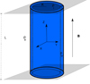 |
Fig. 1. Schema of the coronal flux tube model. The two gray planes located at the ends of the tube represent the solar photosphere where the magnetic field is anchored. |
The coronal loop equilibrium density is nonuniform in the transverse direction only, namely
 (1)
(1)
where r is the radial coordinate, ρi is the density in the uniform inner core, ρe is the uniform external density, and ρtr(r) is the density in a nonuniform transitional layer of thickness l that continuously connects both uniform regions as
![Mathematical equation: $$ \begin{aligned} \rho _{\mathrm{tr} }(r) = \frac{\rho _{\mathrm{i}}}{2}\left\{ \left[1+\frac{\rho _{\rm e}}{\rho _{\mathrm{i}}}\right]-\left[1-\frac{\rho _{\rm e}}{\rho _{\mathrm{i}}}\right]\sin \left[\frac{\pi }{l}\left(r-R\right)\right]\right\} . \end{aligned} $$](/articles/aa/full_html/2021/04/aa40161-20/aa40161-20-eq2.gif) (2)
(2)
The allowed values of l range from l = 0 (abrupt transition) to l = 2R (fully nonuniform loop). We set the equilibrium gas pressure to be a constant everywhere, namely p0, so that the plasma  , where μ is the magnetic permeability. The radial profiles of the equilibrium Alfvén speed,
  , and the equilibrium sound speed,
  , where γ is the adiabatic constant, are displayed in Fig. 2 for a particular set of parameters.
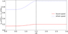 |
Fig. 2. Radial profiles of equilibrium Alfvén and sound speeds in a loop with l/R = 1 and ρi/ρe = 2. The values are normalized with respect to the external Alfvén speed. The vertical dashed lines denote the boundaries of the nonuniform layer. |
2.2. Numerical code
We used the PLUTO code (Mignone et al. 2007) to solve the three-dimensional (3D) ideal MHD equations with a finite-volume, shock capturing spatial discretization on a structured mesh. The equations are as follows:
 (3)
(3)
 (4)
(4)
 (5)
(5)
 (6)
(6)
In these equations,  denotes the total derivative, ρ is the mass density, v is the velocity, p is the gas pressure, and B is the magnetic field. Gravity and nonideal terms are neglected.
The code solves Eqs. (3)–(6) in Cartesian coordinates. We used a Roe-Riemann solver (Roe 1981) to compute the numerical fluxes, a second-order parabolic scheme for spatial reconstruction, and a second-order Runge-Kutta algorithm for temporal evolution. The extended GLM method (Dedner et al. 2002) was employed to keep the solenoidal constraint on the magnetic field. Moreover, an adaptive mesh refinement (AMR) strategy was used (Mignone et al. 2012). The use of AMR allows us to decrease the computational cost by using a high resolution in the region of interest while keeping a lower resolution far from the relevant dynamics. The computational box has a base numerical resolution of 100 × 100 × 100 cells, which are distributed uniformly from −3R to 3R in the x-direction and the y-direction, and from −L/2 to L/2 in the z-direction. We included four levels of refinement in which the cells double the resolution from one level to the next so that the maximum effective resolution is 1600 × 1600 × 1600. For typical values of the loop radius, the effective transverse resolution is ∼10 km. The PLUTO criterion for refinement is based on the second derivative error norm (Lohner 1987) of the perturbation of the total energy, that is, the total energy of the system less the internal and magnetic energy of the background.
Regarding the boundary conditions, we consider outflow conditions, that is, zero gradient, for the pressure, density, the x- and y-components of the magnetic field, while zero velocities are imposed at all boundaries. Concerning the conditions for the z-component of the magnetic field, Bz, we also considered outflow conditions at the lateral boundaries, but Bz is fixed to the equilibrium value, B0, at the bottom and top boundaries, that is, at z = ±L/2, in order to implement the line-tying of the field lines at the photosphere. With these boundary conditions, we checked the nonexistence of significant reflections at the lateral boundaries of the domain during the simulations. Furthermore, a background splitting technique (Powell 1994) was used, which has the advantage that only the magnetic field perturbation over the background magnetic field is evolved by the code.
A recent investigation by Soler et al. (2021) shows that coronal loop torsional oscillations excited by a photospheric broadband driver are dominated by the longitudinal fundamental mode of the loop. In view of this result, we imposed an initial condition for the velocity that aims to excite the longitudinally fundamental mode of standing torsional Alfvén waves. To do so, we imposed the following purely azimuthal velocity field at t = 0:
 (7)
(7)
where v0 is the maximum velocity amplitude and A(r) contains the radial dependence. We shall use the particular form A(r) = A0rexp[−(r2/σ2)] with σ = 0.9R and  is a constant that we obtain from imposing that the maximum value of the velocity is equal to the prescribed value, v0. We note that most of the results discussed in this paper would remain practically unchanged if a different dependence for A(r) was used.
3. Quasi-linear theoretical analysis
Before analyzing the results of the full numerical computations, the purpose here is to solve Eqs. (3)–(6) in an analytic approximated manner when the standing torsional Alfvén waves behave quasi-linearly. These approximate solutions can help us understand the full nonlinear evolution. To do so, we applied a regular perturbation theory (see, e.g., Ballester et al. 2020). In the case of propagating torsional Alfvén waves, a weak nonlinear analysis using the second order thin flux tube approximation can be found in Shestov et al. (2017).
We define the parameter ε ≡ v0/vA, e where vA, e is the external Alfvén speed. Then, assuming ε ≪ 1, we write
where the subscript 0 denotes a background quantity, and the prime ′ denotes a small perturbation. We substituted these expressions into Eqs. (3)–(6) and separated the terms according to their order in ε. The first-order equations in ε govern  , and
, and  , so they describe linear torsional Alfvén waves. The second-order equations in ε2 govern p′, ρ′, and
  and describe nonlinear effects as the ponderomotive force, and the coupling of Alfvén waves with slow magnetoacoustic waves.
3.1. First-order equations: Transverse dynamics
By combining the first-order equations for  and
and  , we can arrive at an equation involving
  alone, namely
 (8)
(8)
where vA, 0(r) is the equilibrium Alfvén velocity, which we recall is a function of the radial direction. Equation (8) is the 1D wave equation with phase velocity equal to the Alfvén speed. We note that in our formalism the actual amplitude of the azimuthal velocity perturbation is  . Equation (8) can be solved for the longitudinally fundamental mode by taking into account the prescribed boundary and initial conditions. The solution is
![Mathematical equation: $$ \begin{aligned} \varepsilon {v}_{\varphi}^\prime ={v}_{0}A(r)\cos \left(\frac{\pi }{L}\; z\right)\cos [\omega _{A}(r) t], \end{aligned} $$](/articles/aa/full_html/2021/04/aa40161-20/aa40161-20-eq22.gif) (9)
(9)
where  is the radially-dependent Alfvén frequency. In turn, the azimuthal magnetic field perturbation is
![Mathematical equation: $$ \begin{aligned} \varepsilon B_{\varphi }^\prime =-B_{0}\frac{{v}_{0}}{\omega _{A}(r)}\frac{\pi }{L} A(r)\sin \left(\frac{\pi }{L}\; z\right)\sin [\omega _{A}(r) t]. \end{aligned} $$](/articles/aa/full_html/2021/04/aa40161-20/aa40161-20-eq24.gif) (10)
(10)
Equations (9) and (10) evidence that standing torsional Alfvén waves excited by the initial perturbation oscillate with the local Alfvén frequency. In the transitional layer, the frequency is nonuniform across the coronal loop. As a result, waves living on adjacent radial positions, excited in phase by our initial condition, will become out of phase as time passes. This is the well-known process of phase mixing (see e.g., Heyvaerts & Priest 1983; Nocera et al. 1984; De Moortel et al. 2000; Smith et al. 2007). Phase mixing continuously decreases the length scale of the disturbances across the loop. In Fig. 3, we illustrate how the azimuthal velocity perturbation is affected by phase mixing in the inhomogeneous region of the flux tube with time. The transverse length scales of the perturbation in the homogeneous inner core and the homogeneous external plasma remain the same at all times. However, the length scale decreases with time in the transitional layer.
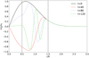 |
Fig. 3. Azimuthal component of the velocity perturbation normalized with respect to the initial amplitude as a function of the radial position at various times. We used l/R = 1, ρi/ρe = 2, L/R = 10, and z = 0. Time is normalized as tvA, e/R. The vertical dashed lines denote the boundaries of the nonuniform layer. |
Following Mann et al. (1995), the effective wave number across the loop can be estimated by
 (11)
(11)
With time, the effective wave number increases. In ideal MHDs, this process works indefinitely. However, in dissipative MHDs, dissipation becomes important for sufficiently high wave numbers at sufficiently long times. Thus, phase mixing transports energy from large to small scales until those small scales can be efficiently dissipated (see, e.g., Ebrahimi et al. 2020). Here, we cannot study the dissipation phase because we restricted ourselves to ideal MHDs.
3.2. Second-order equations: Longitudinal dynamics
In a similar way to what was described in the previous subsection, we combined the second-order equations for  , ρ′, and p′ to obtain an equation for the z-component of the velocity perturbation, namely
 (12)
(12)
where cs, 0(r) is the equilibrium sound speed. Equation (12) is the 1D wave equation with phase velocity equal to the sound speed. We note again that the actual amplitude of the longitudinal velocity perturbation is  . We see the presence of a force term on the right-hand side of Eq. (12), which depends on the perturbation of the magnetic pressure associated with the Alfvén waves. The general solution to Eq. (12) is the sum of the particular and the homogeneous solutions. The homogeneous solution is physically related to the slow magnetoacoustic waves that can propagate freely along the loop at the sound speed. We are not interested in this solution. Conversely, the particular solution is related to the nonlinear longitudinal dynamics associated with the Alfvén waves. In the case that
  is given by Eq. (10), the particular solution to Eq. (12) can be found by direct integration (see, e.g., Martínez-Gómez et al. 2018), namely
![Mathematical equation: $$ \begin{aligned}&\varepsilon ^{2}{v}_{z}^\prime =-{v}^{2}_{0}\frac{A^{2}(r)}{8c_{\mathrm{s},0}(r)}\left[\frac{{v}^{2}_{A,0}(r)}{{v}^{2}_{A ,0}(r)-c^{2}_{\mathrm{s},0}(r)}\right]\sin {\left(\frac{2\pi }{L} z\right)} \nonumber \\&\qquad \qquad \times \Bigg \{\sin \left[\frac{2\pi }{L} c_{\mathrm{s},0}(r) t\right]-\frac{c_{\mathrm{s},0}(r)}{{v}_{A ,0}(r)}\sin \left[2\omega _{A }(r)t\right]\Bigg \}. \end{aligned} $$](/articles/aa/full_html/2021/04/aa40161-20/aa40161-20-eq30.gif) (13)
(13)
Considering the low-β plasma regime so that cs, 0(r) ≪ vA, 0(r), Eq. (13) can be simplified as
![Mathematical equation: $$ \begin{aligned} \varepsilon ^{2} {v}_{z}^\prime \approx -{v}^{2}_{0}\frac{A^{2}(r)}{8c_{\mathrm{s},0}(r)}\sin {\left(\frac{2\pi }{L}\; z\right)}\sin \left[\frac{2\pi }{L} c_{\mathrm{s},0}(r) t\right]. \end{aligned} $$](/articles/aa/full_html/2021/04/aa40161-20/aa40161-20-eq31.gif) (14)
(14)
Equation (14) evidences the existence of longitudinal motions along the flux tube. The amplitude of the longitudinal velocity perturbation depends quadratically on the initial amplitude of the azimuthal velocity, which points out the nonlinear nature of these longitudinal motions. There is a periodic converging (diverging) flow toward (away) from the center of the tube. The result of these flows is the periodic compression and expansion of material around the center of the tube. This is caused by the well-known ponderomotive force (see e.g., Hollweg 1971; Rankin et al. 1994; Tikhonchuk et al. 1995; Terradas & Ofman 2004). The periodicity of these longitudinal motions is L/cs, 0(r), so it depends on the radial position. Thus, the vertical flows associated with the ponderomotive force also become out of phase in adjacent radial positions of the nonuniform layer as time increases. Figure 4 displays the longitudinal velocity normalized as  . With this normalization, the dependence on the initial amplitude is dropped, but the radial structure of the longitudinal flow is kept. For sufficiently long times, a longitudinal velocity shear across the tube in the nonuniform layer is evident.
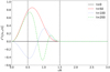 |
Fig. 4. Vertical component of velocity perturbation, normalized as |

3.3. Kelvin-Helmholtz instability: Considerations
The above quasi-linear analysis indicates that the evolution of the torsional Alfvén waves, through phase mixing, results in the occurrence of azimuthal and longitudinal velocity shears in the nonuniform transitional layer. It is well known that a velocity shear in a plasma can drive the KHi (see Chandrasekhar 1961).
The azimuthal shear flows generated by phase mixing can easily develop the KHi, because the velocity shear is perpendicular to the direction of the background magnetic field (see, e.g., Heyvaerts & Priest 1983; Browning & Priest 1984; Soler et al. 2010; Zaqarashvili et al. 2015; Barbulescu et al. 2019). However, the longitudinal shear flows associated with the ponderomotive force cannot develop the KHi since the velocity shear is along the magnetic field. The effect of magnetic tension prevents the instability of sub-Alfvénic flows (Chandrasekhar 1961). Therefore, only the azimuthal shear flows can trigger the KHi in our model.
It is well known by theoretical studies and numerical simulations that the phase-mixing-driven KHi leads to a faster generation of small spatial scales than what the theory of linear phase mixing (Eq. (11)) predicts (see, e.g., Browning & Priest 1984; Pagano et al. 2018; Howson et al. 2020; Van Damme et al. 2020). So, the nonlinear triggering of the KHi can accelerate the energy cascading to the dissipative scales compared with the effect of linear phase mixing alone.
A relevant question that arises is how to determine the onset time of the KHi. In the case that the velocity shear is not steady but periodic, the mathematical analysis is rather involved (see e.g., Kelly 1965; Roberts 1973; Browning & Priest 1984; Hillier et al. 2019; Barbulescu et al. 2019). By assuming strong phase mixing, that is, assuming that the exponential growth time of the KHi is much shorter than the period of the oscillating shear flow, Browning & Priest (1984) provided an approximate expression for the critical onset time. The analysis of Browning & Priest (1984) was done in Cartesian geometry, but it can also be applicable to the cylindrical case studied here. In our model parameters, the expression reads
 (15)
(15)
where A(R) ≈ 0.8 is calculated at a reference point located at the center of the transitional layer, r = R. Equation (15) indicates that the wider the nonuniform layer, the larger the onset time, as is consistent with the fact that phase mixing develops slower in smooth profiles than in sharp ones (Heyvaerts & Priest 1983). In turn, the onset time is inversely proportional to the velocity amplitude of the initial perturbation, which means that the nonlinear triggering of the KHi would occur faster for large amplitudes than for small amplitudes.
Assuming typical values of the coronal Alfvén speed, and the loop length as vA, e= 1000 km s−1, and L = 105 km, the period of the torsional Alfvén wave is P = 2L/vA, e ≈ 3.33 min. In turn, considering a loop radius of R = 3500 km and assuming that the thickness of the nonuniform layer is of the same order, Eq. (15) gives tcrit ≈ 2.92 min for a velocity amplitude of v0 = 100 km s−1 (Kohutova et al. 2020). This simple numerical example indicates that the KHi can be triggered in the loop in a timescale comparable with the period of the torsional oscillations. This implies that the KHi should have a deep impact on the full nonlinear evolution.
4. Numerical simulations
Our aim was to investigate the nonlinear evolution of the phase mixing of torsional Alfvén waves and the triggering of the KHi. We focused on studying how these two mechanisms affect the development of the energy cascade to small scales. Results from the full nonlinear simulations were compared to those from the quasi-linear analytical theory.
Unless otherwise stated, the following reference parameters are used in all simulations: ε = 0.1, ρi/ρe = 2 and L/R = 10, where ε is related to the initial velocity amplitude as v0 = εvA, e. We are aware that the considered value of L/R results in a shorter coronal loop than the loop lengths typically reported in observations. The reason for considering a shorter loop is to speed up the simulation times, since the periods of the torsional oscillations are proportional to L. Considering a longer loop would result in longer simulation times, but the dynamics discussed here would be the same for all practical purposes. The effect of the loop length on the triggering of the KHi is explored in Sect. 4.6.
Concerning the thickness of the nonuniform layer, we considered two cases: a thin-layer case with l/R = 0.4, and a thick-layer case with l/R = 1.5. We considered these two cases because the process of phase mixing, as linear theory predicts, develops at a different pace depending on the inhomogeneity length scale. This is expected to have a strong impact on the nonlinear evolution, including the triggering of the KHi.
In the numerical code, lengths and velocities are normalized with respect to R and vA, e, respectively. Density is normalized with respect to the external density. In turn, time is normalized with respect to the transverse Alfvénic travel time, R/vA, e. In these normalized units, the periods of the internal and external Alfvén waves are  and 20 time units, respectively.
The maximum simulation time is determined by the ability of the four-level AMR scheme to correctly describe the small spatial scales that are generated in the system. To check that, we monitored the total energy integrated in the whole computational domain. We stopped the simulation when the integrated total energy started to decrease significantly, meaning that the developed small scales are beyond the maximum effective resolution of the AMR scheme, and numerical dissipation is becoming significant. By stopping the simulation at that point, we ensured that the simulated dynamics was physically meaningful and minimized the influence that undesirable numerical effects might have. The maximum time that can be correctly simulated according to the energy criterion also coincides with the saturation and subsequent unphysical decrease of the vorticity squared and the current density squared integrated over the whole computational box (this is discussed later, in Sect. 4.2). For the reference parameters given above, the maximum simulation times in the thin-layer and thick-layer cases are t = 86 and t = 150, respectively.
4.1. Nonlinear evolution of phase mixing
Figures 5 and 6 show the temporal evolution of density and the azimuthal component of velocity in a cross-sectional cut at the tube center in the thin-layer and thick-layer cases, respectively. Since the relevant physics is inside and near the flux tube, these figures and the following ones only display cross-sectional cuts in a subdomain where x, y ∈ [−2R,2R], while we recall that the complete numerical domain is larger with x, y ∈ [−3R,3R]. At the beginning of the simulations, the wave evolution agrees with the predictions of quasi-linear theory. As time passes, the alternation between red (positive) and blue (negative) values of the azimuthal component of velocity within the nonuniform layer is a clear evidence that the process of phase mixing is at work (see Heyvaerts & Priest 1983). In the transition region, where the density is nonuniform, adjacent radial positions become out of phase as the simulation evolves, generating azimuthal shear flows and smaller spatial scales across the tube. The development of phase mixing is slower in the thick-layer case than in the thin-layer case because of the smoother Alfvén speed gradient.
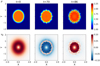 |
Fig. 5. Top: cross-sectional cut of density at the tube center, z = 0, for the thin-layer case at three different simulation times indicated on top of each panel. Bottom: same cut, but for the azimuthal component of velocity. The full temporal evolution is available as an online movie. |
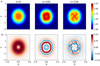 |
Fig. 6. Same as Fig. 5, but for the thick-layer case. We note that the three selected simulation times are different from those of Fig. 5. The full temporal evolution is available as an online movie. |
The cross-sectional cut of density initially shows no significant density variations, which is consistent with the fact that torsional Alfvén waves are incompressible in the linear regime. A slight periodic compression and expansion of the tube area can be seen, owing to the ponderomotive force as the analytical second-order perturbation predicts (see also Hollweg 1971). A better insight into the effect of the ponderomotive force can be visualized in Fig. 7. There, we show the temporal evolution of density and the longitudinal component of velocity in a longitudinal cut along the loop for the thick-layer case. The periodic density enhancement around the tube center caused by the ponderomotive force is evident. The wavelength of the periodic longitudinal flows is half that of the torsional Alfvén wave and their amplitude depends quadratically on the amplitude of the azimuthal perturbation. The longitudinal component of velocity changes sign at the center of the tube, which is a converging/diverging point. These results can be compared to those of Shestov et al. (2017) in the case of weak nonlinear propagating torsional Alfvén waves. In their case, the average of the longitudinal component of velocity along the loop is positive. However, since the present simulations correspond to the fundamental mode of standing waves, the longitudinally averaged velocity, vz, in our case is zero. We note that the longitudinal velocity develops shear in the nonuniform layer when phase mixing evolves. As is consistent with analytic theory, these longitudinal shear flows are much slower than the corresponding azimuthal flows.
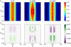 |
Fig. 7. Longitudinal cuts of density (top) and longitudinal component of velocity (bottom) at y = 0 for the thick-layer case at the same simulation times as in Fig. 6. The full temporal evolution is available as an online movie. |
Later in the evolution, the system undergoes a change from a linear to nonlinear regime. The KHi is triggered by the azimuthal shear flows and develops in the nonuniform layer, as the middle and the right panels of Figs. 5 and 6 evidence. No KHi associated with the longitudinal shear flows is seen in Fig. 7. Consistently, the KHi develops earlier and faster in the thin-layer case because of the larger phase-mixing-driven shear flows. Similarly to the results of Guo et al. (2019) for their torsional Alfvén wave model, we observe that the KHi is first triggered around the middle of the transition region, that is, at r ≈ R, where the strongest shear flows occur. Hence, the onset of the KHi appears to be a local phenomenon that does not affect, initially, the entire nonuniform region. In connection to this, we interestingly notice in the bottom right panel of Fig. 6, corresponding to the thick-layer case, that the KHi is only developing at that instant in a relatively small part of the whole nonuniform layer, while the linear phase mixing continues to operate in the remaining transitional region.
The most obvious consequence of the onset of the KHi is the formation of eddies clearly seen in the evolution of density. The internal and external plasmas mix as a result of these vortical motions. As time increases, eddies break down to form smaller and smaller structures. The instability drives the flux tube to a turbulent state. The extent of the turbulent zone increases with time and surpasses the width of the nonuniform layer. At sufficiently long times beyond those simulated here, the whole tube should become turbulent (see Karampelas & Van Doorsselaere 2018 for simulations of kink waves). The simulations show that the turbulence develops in the transverse plane to the magnetic field only. Figure 7 evidences that there is no eddy formation in the longitudinal direction. Thus, we are in a clear situation of nearly 2D Alfvénic turbulence in which the spatial scales perpendicular to the background magnetic field are much smaller than the scales in the magnetic field direction. As shown in Sect. 4.4, this has implications for the energy cascade scaling law.
Since we are studying the fundamental standing mode, the amplitude of the torsional oscillations is maximal at the middle of the tube (z = 0) and zero at the tube ends (z = ±L/2) because of the line-tying condition. Consequently, it is at the z = 0 plane that turbulence develops fastest and strongest. Conversely, at z = ±L/2 the KHi is not triggered, so there is no development of turbulence.
The nonlinear evolution of the torsional oscillations shares many similarities with that of kink MHD modes (see, e.g., Terradas et al. 2008, 2018; Antolin et al. 2015; Magyar & Van Doorsselaere 2016; Howson et al. 2017; Karampelas et al. 2019; Antolin & Van Doorsselaere 2019). In our case, the tube is not displaced laterally as it is for a kink mode, but the KHi develops in a similar fashion. In the case of the kink mode in a transversely nonuniform tube, a previous step is the energy transfer from the global lateral oscillation to localized Alfvén modes in the nonuniform layer owing to resonant absorption. (see, e.g., Terradas et al. 2006; Goossens et al. 2011; Arregui et al. 2011; Soler & Terradas 2015). These localized Alfvén modes with kink azimuthal symmetry are the ones that phase mix and eventually trigger the KHi. We note that the KHi can also be triggered by the kink mode even in tubes with an abrupt density transition (see Antolin & Van Doorsselaere 2019). In that case, resonant absorption does not happen initially, and it is the own azimuthal shear associated with the global kink mode perturbations that triggers the KHi. For the torsional oscillations studied here, there is no global mode, and the resonant absorption mechanism does not occur. In our case, Alfvén modes with torsional azimuthal symmetry are already excited by the initial condition, so the phase mixing starts to operate from the beginning of the simulation.
4.2. Increase of vorticity and current density
Two parameters that help us illustrate the important effect of the KHi on the torsional oscillation evolution are vorticity, ω = ∇ × v, and current density, j = μ−1∇×B. We find that the KHi dramatically increases both quantities because of the small scales that rapidly show up once the KHi is triggered. We compute the vorticity squared and the current density squared in a cross-sectional cut of the tube. The cut is done at the tube center, z = 0, for the vorticity and near one tube end, z ≈ L/2, for the current density. The reason for choosing these different cuts is the different spatial dependences of the two parameters along the tube: vorticity is maximal at the tube center and zero at the ends, while the opposite applies to current density. Figures 8 and 9 show these results for the thin-layer and thick-layer cases, respectively. We used logarithmic scale to better visualize the important change in the magnitude of both quantities.
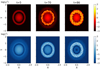 |
Fig. 8. Top: cross-sectional cut at z = 0 of vorticity squared (in logarithmic scale) for the thin-layer case at three different simulation times indicated above each panel. Bottom: same, but for the current density squared at z ≈ L/2. The straight lines seen in some panels are visualization artifacts at the boundaries of different AMR patches. These artifacts are not present in the actual simulation data. The full temporal evolution is available as an online movie. |
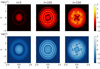 |
Fig. 9. Same as Fig. 8, but for the thick-layer case. We note that the three selected simulation times are different from those of Fig. 8. The full temporal evolution is available as an online movie. |
As expected, both vorticity and current density initially agree with the results from linear analytic theory. Thus, they evolve in the nonuniform layer, and their values increase as a result of phase mixing alone. However, once the KHi sets in, analytic, and numerical results start to differ substantially. The full nonlinear evolution is characterized by the generation of very fine structures in both vorticity and current density, and by a dramatic increase of their magnitudes. Figure 10 shows a comparison between linear analytic results and nonlinear numerical results for the vorticity squared at the final frame of the simulations. The analytic vorticity is computed with the azimuthal velocity component given in Eq. (9). The comparison in the case of the current density squared reveals similar results and for the sake of simplicity is not shown here. The very fine structures in vorticity and current density associated with the KHi can also be seen in previous works of nonlinear kink oscillations (see e.g., Antolin et al. 2014; Howson et al. 2017; Antolin & Van Doorsselaere 2019) where the spatial distribution is slightly different because of the different azimuthal symmetry of the perturbations.
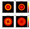 |
Fig. 10. Top: cross-sectional cut at z = 0 of vorticity squared (in logarithmic scale) for the thin-layer case at the final simulation time. The left and right panels correspond to the nonlinear numerical results and the linear analytic results, respectively. Bottom: same, but for the thick-layer case. |
The change of magnitude of vorticity squared and current density squared can be better studied by integrating both quantities over the whole computational domain as
 (16)
(16)
 (17)
(17)
Figure 11 shows the evolution of Ω2 and I2 for both thin-layer and thick-layer cases. A comparison with the values predicted by linear theory is also included.
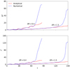 |
Fig. 11. Vorticity squared (top panel) and current density squared (bottom panel) integrated over the whole computational domain as a function of simulation time for both thin-layer (l/R = 0.4) and thick-layer (l/R = 1.5) cases. Red solid lines correspond to linear analytic results, and blue dashed lines correspond to nonlinear numerical results. Vorticity is normalized to the value at t = 0. No normalization is needed for current density since it vanishes at t = 0. |
We find that both integrated quantities increase with time following a slightly oscillatory pattern, and numerical and analytic results initially agree. The increase is faster in the thin-layer case than in the thick-layer case. Such a result is consistent with the behavior of phase mixing (see, e.g., Heyvaerts & Priest 1983). Hence, the initial increase of vorticity and current density is predicted by linear theory and is caused by phase mixing alone. However, once the KHi is triggered in the numerical simulations, both integrated quantities suffer a dramatic increase that is not predicted by linear theory. At the end of the simulations, the numerical values of Ω2 and I2 are significantly larger than those of linear theory.
Previous works have studied vorticity in the case of nonlinear kink waves (e.g., Terradas et al. 2008; Antolin et al. 2015; Karampelas et al. 2017; Howson et al. 2020). Guo et al. (2019) studied the average z-component of vorticity squared integrated at the loop apex for both torsional Alfvén and kink waves. As in these works, we verified that the main contribution to the vorticity squared is its z-component due to the development of strong gradients in the transverse components of velocity. Guo et al. (2019) and Howson et al. (2020) found increasing oscillations in vorticity with time not only due to phase mixing and the KHi, but also because of the continuous driver used to excite the waves. Conversely, here we impose an initial perturbation and let the system evolve. Therefore, in our case, the generation of vorticity and current density is because of phase mixing in the linear regime and the KHi in the nonlinear regime, with no influence from an external driver.
At this point, we feel it is relevant to stress the importance of using a sufficiently high resolution to correctly capture the very fine scales generated because of the KHi. For instance, Fig. 2 of Antolin et al. (2015) shows a cross-sectional cut of the z-component of the vorticity and current density at the apex of a cylindrical tube representing a prominence thread oscillating in the kink mode. They show the same results with low resolution (left panels) and high resolution (right panels). Their high-resolution simulation is able to describe smaller scales and shows higher values of current density and vorticity. Another example can be found in Howson et al. (2017), where they compare ideal MHD simulations of nonlinear kink oscillations with simulations including viscosity and/or resistivity. Their Fig. 6 shows that in the ideal MHD simulation, vorticity increases drastically due to the development of KHi, but after t ≈ 700 s it saturates and decreases, presumably owing to numerical dissipation, which also explains the loss of kinetic energy for t > 700 s (see their Fig. 9). In another ideal simulation but at lower resolution, they show that the saturation of vorticity happens earlier. Simulations including physical dissipation show similar results, pointing out that physical and numerical dissipation can play equivalent roles. If dissipation is strong enough, the KHi can be delayed or can even be suppressed altogether. In the case of torsional Alfvén waves, Guo et al. (2019), in their Fig. 2, did not find the significant increase of vorticity that we obtained after the onset of the KHi. Possible explanations may be that the KHi had not yet completely developed in their simulation, or that numerical diffusion plays a role.
To further investigate the influence of numerical resolution, we have repeated the simulation for the thin-layer case, but using fewer levels of refinement in the AMR scheme. The lower the number of levels, the lower the effective resolution. In Fig. 12, we show the evolution with time of vorticity squared integrated over the whole computational box for these test simulations. These results are also compared to those of linear theory. In all cases and for comparison purposes, the end time of the simulations has been set to that of the four-level simulation. We find that all simulations behave similarly in the linear regime, but after the system transits to the nonlinear regime and the KHi is triggered, the higher the resolution, the larger the increase of vorticity. We obtain the interesting result that the simulations with only one or two levels of refinement are not even able to correctly recover the linear results. In those cases, numerical dissipation is also strong enough to prevent the onset of the KHi, in agreement with Howson et al. (2017). These results confirm the need to use high resolutions to correctly describe the evolution of the KHi and to minimize the significant impact of numerical diffusion.
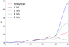 |
Fig. 12. Vorticity squared integrated over the whole computational domain as a function of simulation time for the thin-layer case. The various lines correspond to simulations with different levels of refinement in the AMR scheme: 1 (black dot-dashed line), 2 (brown dotted line), 3 (green dashed line), and 4 (blue solid line). For comparison purposes, the linear analytical value is also shown (red dashed line). Vorticity is normalized to the value at t = 0. |
4.3. Investigating the onset of the KHi
The aim here is to compare the onset time of the KHi obtained from the simulations with the theoretical one predicted by Browning & Priest (1984). The problem with the simulations is to find an objective criterion to define the onset time. The behavior with time of the integrated vorticity squared can be a way to estimate the onset time from the simulation data. As seen in Fig. 11, the slope of the ascending trend of vorticity changes and deviates from the linear result at a specific time that can be associated with the onset of the KHi. We denote this time as τKH. The integrated current density squared also displays a slope change at the same time as vorticity, approximately, but we used the vorticity data. Then, by visual inspection, we determined that τKH ≈ 66 in the thin-layer case, and τKH ≈ 120 in the thick-layer case. Moreover, we compared these estimated onset times with Eq. (15) obtained by Browning & Priest (1984) in the strong phase-mixing limit. Equation (15) gives tcrit ≈ 20 in the thin-layer case and tcrit ≈ 75 in the thick-layer case. Therefore, Eq. (15) predicts that the KHi is triggered earlier than the simulations apparently show.
A reason for this discrepancy may lie in the strong phase-mixing approximation behind Eq. (15). When this approximation is relaxed, we can use the following method provided in Sect. 4 of Browning & Priest (1984) to adapt Eq. (15) to the weak phase-mixing case:
 (18)
(18)
where Tcrit is their dimensionless onset time, which depends on the parameter Ω1 that, in our notation, is
 (19)
(19)
with kz = π/L the parallel wave number to the magnetic field. Figure 7 of Browning & Priest (1984) shows the dependence of Tcrit with Ω1. The strong phase-mixing limit should correspond to the case Ω1 ≫ 1 so that Tcrit → 4 and Eq. (15) is recovered. We note that in their Sect. 4, Browning & Priest (1984) considered the particular case vA, i = 0.5vA, e, while in our model  . However, we assume that the results in their Fig. 7 remain approximately valid in our case. According to the parameters of our simulations, we have Ω1 = 2π/5 ≈ 1.26 for the thin-layer case and Ω1 = 3π/2 ≈ 4.71 for the thick-layer case. Therefore, we are far from the strong phase-mixing limit, especially in the thin-layer case. Using Fig. 7 of Browning & Priest (1984), we approximately determine that Tcrit ≈ 8 for the thin-layer case, so tcrit ≈ 40 according to the modified Eq. (18). This critical time approaches the value inferred from the integrated vorticity slope change but is still lower. For the thick-layer case, the determination of Tcrit is more problematic since Fig. 7 of Browning & Priest (1984) stops at Ω1 = 2 where Tcrit ≈ 7. As Browning & Priest (1984) explained, we can assume that Tcrit approaches the strong phase-mixing value, Tcrit = 4, asymptotically when Ω1 ≫ 1, but for Ω1 ≈ 4.71 we are probably still far from the limit. An educated guess would be to assume that Tcrit is somewhere between the asymptotic value and the last value seen in Fig. 7 of Browning & Priest (1984). So, we roughly approximate Tcrit ≈ 5, which results in tcrit ≈ 94 in the thick-layer case according to the modified Eq. (18). This value is again lower than that obtained from the vorticity data.
One may ask why the critical times of Browning & Priest (1984) are systematically smaller than those inferred from the slope change of the integrated vorticity squared, even when the strong phase-mixing limit is relaxed. The answer to this question is that tcrit of Browning & Priest (1984) corresponds to the time at which the KHi is locally excited within the nonuniform later, while our τKH should be associated with a time for which the KHi has developed enough to globally impact the flux tube dynamics. We recall that τKH is obtained from a quantity that has been integrated over the whole tube, so that local effects are probably blurred. To check this statement, we need a method to estimate, from the simulations, the time at which the KHi is first locally triggered in the nonuniform layer. The evolution of density (see again Figs. 5 and 6) indeed shows that the initial local distortion of density associated with the KHi happens for a somewhat earlier time than τKH, but we need a more robust approach.
Inspired by Terradas et al. (2018; see also Antolin & Van Doorsselaere 2019), we studied the excitation of different azimuthal wave numbers using the azimuthal and radial components of velocity in the transitional layer. We considered a cross-sectional cut at the center of the tube, z = 0, and extracted, from the simulations, the values of the azimuthal and radial components of velocity at the middle of the transition region, r = R, as functions of the azimuthal angle from 0 to 2π. After that, we applied the discrete Fourier transform to the data using the fast Fourier transform (FFT) algorithm in 1D (Cooley & Tukey 1965). Following the notation of Terradas et al. (2018), the discrete Fourier transform can be defined as
 (20)
(20)
where N is the number of samples (points), g(k) is the angular sampling of the azimuthal/radial velocity, and p = 0, …, N − 1 is an integer that plays the role of the azimuthal wave number. p = 0 is the torsional or sausage mode, p = 1 is the kink mode, and p ≥ 2 are the fluting modes (see, e.g., Edwin & Roberts 1983). We find that the Fourier coefficients, G(p), are complex except for p = 0, which is always real. Terradas et al. (2018) found that the Fourier coefficients associated with the azimuthal component of velocity were purely imaginary, while those associated with the radial component were real. They explained that this result is due to parity rules of their initial condition since they only excite the p = 1 kink mode at t = 0. Nonetheless, we excited the p = 0 torsional mode at t = 0, and those parity rules may not apply in our case.
The results of the azimuthal Fourier analysis are shown in Fig. 13 for the thin-layer case and in Fig. 14 for the thick-layer case. In both figures, the top (bottom) panels show the real part of the Fourier coefficients as functions of time obtained from the azimuthal (radial) component of velocity. The studied azimuthal wave numbers are p = 0 (torsional), p = 1 (kink), p = 2 (first fluting), p = 3 (second fluting), p = 4 (third fluting), and p = 12 (eleventh fluting). Additionally, we also plot the result predicted by linear theory, which only contains the p = 0 torsional mode. With vertical dashed lines, we indicate the values of tcrit and τKH for each case.
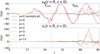 |
Fig. 13. Top panel: real part of the Fourier coefficients with p = 0, 1, 2, 3, 4, and 12 as functions of the computational time for an angular sampling of the azimuthal component of velocity at r = R and z = 0 in the thin-layer case. The two vertical dashed lines correspond to the critical time of Browning & Priest (1984), tcrit = 40, and the onset time inferred from the integrated vorticity slope change, τKH = 66. The linear analytic result, where only the p = 0 mode is present, is overplotted for comparison. Bottom panel: same as top panel but for the radial component of velocity. |
Concerning the azimuthal component of velocity, the p = 0 Fourier coefficient is dominant during the linear regime, while the others are negligible. This remains the case until the development of KHi, which excites higher azimuthal wave numbers. This agrees with the results of Terradas et al. (2018) and Antolin & Van Doorsselaere (2019). We obtain an amplification of the p = 0 Fourier coefficient as time increases. This amplification is due to phase mixing alone, as can be seen by comparing the numerical result with that from linear theory. After the KHi is triggered, not all azimuthal wave numbers are equally excited at a given time. The larger the value of p, the later these modes are excited. Toward the end of the simulations and especially in the thin-layer case, we observe that the amplitude of the Fourier modes with high azimuthal wave numbers can even become comparable to that of the torsional mode because of the nonlinear evolution of the KHi into turbulence. To fully understand why some azimuthal wave numbers are excited before others, a similar theoretical study to that of Browning & Priest (1984) but in cylindrical geometry and with time-varying flows is required. This is beyond the scope of the present paper.
We verified (not shown here) that the excitation of high-order azimuthal wave numbers initially occurs in the nonuniform region only. There is no signature of azimuthal wave numbers other than p = 0 in the uniform core of the tube where the triggering of the KHi is not possible. However, once the KHi is fully developed and the whole tube is driven to a turbulent state, high-order azimuthal wave numbers can be present everywhere.
Regarding the radial component of velocity, we consistently see that all Fourier modes vanish at t = 0 and remain negligible in the linear regime before the excitation of the KHi, since the oscillations are strictly polarized in the azimuthal direction at the beginning. After the triggering of the KHi, nonzero amplitudes of G(p) for the radial component of velocity are found, with the p = 0 mode being the largest contributor.
Recovering the results of the density evolution shown in Figs. 5 and 6, one could tentatively infer that the dominant azimuthal wave numbers are p = 12 and p = 4 in the thin-layer and thick-layer cases, respectively, merely by counting the number of big vortices that appear when the KHi develops. This simple estimation can be compared with the azimuthal Fourier analysis. In Fig. 14, we can see that the p = 4 mode is one of the most relevant modes after the torsional p = 0 mode in the thick-layer case at the end of the simulation, especially for the radial component of velocity. Conversely, in the thin-layer case (Fig. 13), the p = 12 mode is hardly excited in either velocity component. There are several reasons that may explain this discrepancy. For instance, we note that the analysis of azimuthal modes preformed here does not use the density but the velocity components, and is done at a particular radial position, r = R. We checked (not shown here) that the relative amplitude of a particular Fourier mode depends on both the variable used in the analysis and the radial position where the azimuthal sampling is done.
In both thin-layer and thick-layer cases, the critical times of Browning & Priest (1984), tcrit, approximately coincide with the times for which azimuthal wave numbers with p ≠ 0 start to grow within the nonuniform layer. This result confirms us that the onset times obtained from the change of trend in the integrated vorticity squared, τKH, overestimate the actual local onset of the KHi. Instead, τKH should be interpreted as a timescale for which the KHi starts to have a global effect on the flux tube dynamics. In Sect. 4.6, we detail a study of the effect of various model parameters on the value of τKH.
4.4. Turbulent energy cascade to small scales
The results of the numerical simulations clearly indicate that the generation of small spatial scales speeds up when the KHi is triggered, and turbulence develops thereafter. Here, we study how the energy cascades from large to small scales and compare the efficiency of this process in the linear and nonlinear regimes. For this purpose, we calculated the amplitude spectrum of the averaged energy of the perturbations as a function of time. The procedure is described below.
First, we compute the sum of the magnetic and kinetic energy of the transverse perturbations to the background magnetic field in a subdomain where x, y ∈ [−2.03R,2.03R]. Then, we average the energy in y- and z-directions and retain the dependence in the x-direction only. We denote this averaged energy as E̅(x,t). After that, we apply the continuous Fourier transform, which is discretized due to the limited numerical resolution as
 (21)
(21)
where N is the number of samples, k⊥ is the perpendicular wave number, and Δx and x0 are the spatial resolution and the upper limit of the selected subdomain in the x-direction, respectively. The summatory in Eq. (21) is exactly the 1D discrete Fourier transform, which we computed using the FFT algorithm (Cooley & Tukey 1965). Finally, we calculate the modulus of E̅F(k⊥,t), and normalize it with respect to the maximum value in the spectrum at each time. Moreover, to compare with linear results, we repeat this computation, but with the analytic formulas in the linear regime. For simplicity, this analysis was done in the thin-layer case alone. The results of the Fourier transform are plotted in Fig. 15 corresponding to the final frame of the simulation. In Fig. 15, with a vertical line, we show the maximum theoretical wave number across the loop, kmax, generated by phase mixing (we used Eq. (11)). The results of the analytic spectrum for k⊥ > kmax are unphysical and must be ignored because phase mixing cannot generate such large wave numbers (Mann et al. 1995). This is just a numerical artifact caused by the FFT routine when it is forced to be extended to larger wave numbers in order to obtain the same wave-number range as in the numerical spectrum.
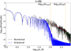 |
Fig. 15. Amplitude spectrum (arbitrary units) of the averaged total energy of the perturbations for the thin-layer case at the end of the simulation for both numerical and linear analytic results. The vertical dot-dashed orange lines denote the maximum phase-mixing-generated wave number, kmaxR ≈ 105, obtained from Eq. (11), and an estimated wave number for which numerical diffusion starts to play a role, kdiffR ≈ 500. The red line is a least-squares linear fit for kmax < k⊥ < kdiff in log-log scale whose slope is −2.07 ± 0.02. The green line is the same fit but for k⊥ > kdiff, whose slope is −3.28 ± 0.07 |
As expected, we verified that at t = 0 and during the initial simulation frames, analytical and numerical spectrums coincide (not shown here). This is the case until the onset of the KHi. Then, the analytical and numerical spectra start to differ for sufficiently high wave numbers. Interestingly, they differ for a wave number that is somewhat smaller than kmax. This clearly confirms that the development of turbulence produces much smaller scales (higher waver numbers) than what phase mixing alone is capable of. For k⊥ > kmax, the amplitude of the numerical spectrum is much larger than that of the analytic spectrum. In fact, as mentioned before, the amplitude of the analytic spectrum should tend to zero for k⊥ > kmax. Therefore, in the full nonlinear results there is a faster cascading of energy to small scales than in the linear regime.
The numerical simulations show that the KHi drives the loop to a turbulent state and that turbulence speeds up the energy transport from large to small scales. One question that may arise is whether the energy cascading obtained here agrees with what is expected under conditions of turbulence. According to turbulence theory (see, e.g., Chorin 1994; Frisch 1995; Pope et al. 2000; Schnack 2009), spectra can be divided into two main regions: the energy-containing range and the universal equilibrium range, which, in turn, contains the inertial subrange and the dissipation range. The scaling of the energy with the wave number in the inertial subrange can give us the information we are looking for.
The wave number that separates the inertial subrange from the energy-containing range is difficult to estimate because it depends on the characteristics of the problem (Pope et al. 2000; Bluteau et al. 2011). A typical spectrum for a driven system should contain a region of small wave numbers where energy increases with the wave number before it decreases in the inertial subrange (Biskamp 2003). However, we do not have this increase in our spectrum because we did not use a driver, which would input energy continuously. Instead, we imposed an initial perturbation. To make sure that the considered wave numbers fell entirely within the inertial subrange, we considered k⊥ > kmax. This choice also excludes the effect of linear phase mixing. On the other hand, the dissipation range, where the energy is dissipated, cannot be studied in ideal MHDs. Under coronal conditions, the critical wave number between the inertial subrange and the dissipation range should be larger than the wave numbers considered in Fig. 15. Nevertheless, although small, some numerical diffusion is at work. To eliminate any effect numerical dissipation may have, we excluded wave numbers higher than an estimated numerical diffusion wave number, kdiff. Therefore, we assume that the inertial subrange approximately corresponds to kmax < k⊥ < kdiff. For the case of Fig. 15, we have kmaxR ≈ 105, and we visually estimated kdiffR ≈ 500 from an evident slope change in the spectrum at high wave numbers (see below).
In order to determine the approximate slope of the numerical spectrum in the inertial subrange, we performed a least-squares linear fit in log-log scale. The result of the best fit is overplotted in Fig. 15. The adjusted slope is −2.07 ± 0.02. On the other hand, an equivalent fit performed in Fig. 15 for k⊥ > kdiff reveals a steeper slope of −3.28 ± 0.07, which is consistent with the assumption that for k⊥ > kdiff numerical diffusion plays a role in this high-wave-number range.
We note that the fit slope in the inertial subrange may change if the estimated boundary wave numbers, namely kmax and kdiff, are modified. We are aware that the choice of these boundary wave numbers is not free from a certain degree of arbitrariness. In spite of this and considering the limitations of this rough estimation, the obtained slope of ≈ − 2 differs from the so-called Kolmogorov law of −5/3 (see e.g., Kolmogorov 1941; Frisch 1995; Pope et al. 2000). The Kolmogorov scaling law is a universal property in hydrodynamic turbulence and also appears in strong MHD turbulence (see, Biskamp 2003; Schnack 2009). The obtained slope is also different for the Iroshnikov-Kraichnan law of −3/2 because of isotropic Alfvénic turbulence (Iroshnikov 1964; Kraichnan 1965). We note that neither the condition of isotropy nor that of strong turbulence are satisfied in our simulations, which may explain why we obtain a different slope. As discussed by Nazarenko (2011) and Schekochihin et al. (2012); see also, Ng & Bhattacharjee (1997), Galtier et al. (2000), in the case of anisotropic weak Alfvénic turbulence that evolves nearly 2D in the plane transverse to the background magnetic field with k⊥ ≫ k∥, as it is indeed the case of our simulations, the energy spectrum should scale as  . This scaling law is compatible with the approximate slope we fit in Fig. 15 for kmax < k⊥ < kdiff. However, we must warn the reader that the −2 power law discussed in Nazarenko (2011) and Schekochihin et al. (2012) is obtained for unbalanced turbulence arising from wave-wave interaction, while the turbulence in our case is driven by the KHi. Therefore, caution is needed with this comparison of the power law (A. Hillier, priv. comm.).
4.5. Effective Reynolds number
A consequence of the faster generation of small scales owing to turbulence is that the dissipative scales should be reached much before than the theory of linear phase mixing predicts (see Terradas & Arregui 2018). A way to further quantify the differences between linear and nonlinear results is to estimate the effective Reynolds number in the simulations as
![Mathematical equation: $$ \begin{aligned} R_{\rm eff}=\frac{\left|\rho \left[\frac{\partial \mathbf v }{\partial t}+\left(\mathbf v \cdot \nabla \right)\mathbf v \right]\right|}{\left|\rho \nu \left[\nabla ^{2}\mathbf v +\frac{1}{3}\nabla \left(\nabla \cdot \mathbf v \right)\right]\right|}. \end{aligned} $$](/articles/aa/full_html/2021/04/aa40161-20/aa40161-20-eq44.gif) (22)
(22)
The numerator of Eq. (22) is the magnitude of the inertial term, whereas the denominator is the magnitude of the viscous force, with ν the kinematic viscosity (see, e.g., Priest 2012). Using R and vA, e as characteristic length and velocity scales, Eq. (22) gives
 (23)
(23)
for typical values of the parameters in the corona. We recall that we performed ideal MHD simulations, so the viscous term is absent from the equations we actually solved. Assuming that the effect of viscosity, if included, would regardless be small during the considered simulation times because we are still far from the dissipative scales, we can approximately study how the Reynolds number would evolve in our simulations.
Figure 16 shows a cross-sectional cut of the effective Reynolds number at the tube center at the end of the simulation times for both thin-layer and thick-layer cases. In order to compare with the linear theory, we also include the results that we obtained using the theoretical expressions of the velocity in the quasi-linear analysis. We also observed the evolution of Reff with the simulation time (not shown here) before the time plotted in Fig. 16. As expected, numerical and theoretical effective Reynolds numbers are initially similar. As time increases, phase mixing is developed in the nonuniform layer, and Reff varies in the form of concentric rings between minimums and maximums. These minimums of Reff are very local, that is, they only occur in very thin regions within the nonuniform layer.
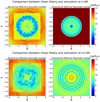 |
Fig. 16. Top: numerical (left) and analytic (right) effective Reynolds number in logarithmic scale at the end time of the simulation in the thin-layer case. These results are calculated in a cross-sectional cut at z = 0. The straight lines seen in the numerical result are visualization artifacts due to the AMR scheme. These artifacts are not present in the actual simulation data. Bottom: same as top panels, but for the thick-layer case. |
When the simulations reach the nonlinear regime, the effective numerical Reynolds number dramatically decreases in the nonuniform layer due to the KHi. The formation of eddies associated with the KHi greatly increases the denominator of Eq. (22), that is, the size of the hypothetical viscous term. As turbulence develops, low values of Reff are found within the entire nonuniform layer. The decrease of Reff is no longer a very local phenomenon, as it happens when phase mixing is operating alone. At the final time of the simulations, the values of Reff are as low as Reff ∼ 106, that is, six orders of magnitude lower than at t = 0. The thick-layer case, where the KHi is less developed than in the thin-layer case, shows an intermediate step in which the dramatic decrease of Reff due to turbulence only occurs in the inner part of the nonuniform region, while in the outermost part of the layer, phase mixing is still at work and larger values of Reff are found.
4.6. Parameter survey
To this point, we considered fixed values for the initial amplitude, ε, the width of the transition region, l/R, the density contrast between the core of the flux tube and the external medium, ρi/ρe, and the loop length, L/R. Here, we explore the effect that each one of these four parameters has on the excitation of the KHi during the nonlinear evolution of the torsional oscillations. To do so, we ran different simulations by keeping three of the parameters fixed and varying the remaining one. We performed 15 different simulations. For each simulation, we computed the vorticity squared integrated over the whole computational domain using Eq. (16) and estimated the value of τKH in each case.
Figure 17 shows the results of the parameter study for fixed ε = 0.1, L/R = 10, and ρi/ρe = 2, and varying l/R = {0.4,0.7,1.0,1.5}. The left panel shows the evolution of integrated vorticity squared as a function of time, where we can clearly identify the linear phase and the subsequent change of slope at t = τKH due to the global onset of the KHi. The right panel shows the estimated values of τKH for every simulation with different l/R. As expected, we find that the onset of KHi is delayed as l/R increases, and, in the linear regime, the slope of the integrated vorticity squared depends on the value of l/R. This is consistent with the fact that the phase-mixing pace depends on the inhomogeneity length scale: it operates faster (slower) when l/R decreases (increases). The strong enough shear flows needed to trigger the KHi occur at a later time as l/R grows. Conversely, after the KHi is triggered, the slope of the integrated vorticity squared is approximately the same for all values of l/R, which points out that the nonlinear evolution of the KHi is less affected by the inhomogeneity length scale.
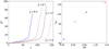 |
Fig. 17. Left panel: vorticity squared integrated over the whole computational domain as a function of the simulation time for ε = 0.1, ρi/ρe = 2.0, L/R = 10, and l/R = {0.4,0.7,1.0,1.5}. The curves are normalized to the integrated vorticity squared at t = 0. Right panel: estimated τKH as a function of the width of the transition region, l/R. |
Figure 18 shows the same analysis, but when l/R = 0.4, L/R = 10, and ρi/ρe = 2 are kept fixed, and we vary ε = {0.06,0.1,0.2,0.25}. As expected, we find that the larger the perturbation amplitude, the earlier the KHi sets in. This is so because larger shear flows are present and the nonlinear regime is more rapidly reached as the amplitude increases. We notice that, as should be the case, all curves in the left panel of Fig. 18 superimpose in the linear regime before the onset of the KHi.
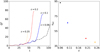 |
Fig. 18. Left panel: same as left panel of Fig. 17, but now the fixed parameters are l/R = 0.4, L/R = 10, and ρi/ρe = 2.0, and we vary ε = {0.06,0.1,0.2,0.25}. Right panel: estimated τKH as a function of the amplitude of the velocity perturbation. |
Finally, Fig. 19 displays the results when l/R = 1.5, L/R = 10, and ε = 0.1 are kept fixed and we vary ρi/ρe = {2,5,6.5,10,13}. The dependence of τKH on the density contrast is not as clear as for the other two parameters. For low-density contrasts, τKH decreases when ρi/ρe increases. However, τKH appears to saturate to a roughly constant value for higher density contrasts. The initial decrease of τKH with ρi/ρe is consistent with the fact that a larger density contrast implies a more abrupt Alfvén speed variation within the nonuniform layer and so a faster development of phase mixing. This seems to be true up to a certain value of the contrast, but the precise value of ρi/ρe becomes irrelevant once it is large enough. We speculate that this behavior may be caused by the functional dependence of the Alfvén speed with the density, namely vA ∼ ρ−1/2.
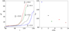 |
Fig. 19. Left panel: same as left panel of Fig. 17, but now the fixed parameters are ε = 0.1, L/R = 10, and ρi/ρe = 2.0, and we vary ρi/ρe = {2,5,6.5,10,13}. Right panel: estimated τKH as a function of the density contrast between the core of the flux tube and the external medium. |
The dependence of τKH with l/R and ε qualitatively agrees with the behavior predicted by the approximate critical time of Browning & Priest (1984) in the strong phase-mixing limit (see Eq. (15)). However, Eq. (15) is independent of the density contrast. The result that τKH turns independent of ρi/ρe for large values of this parameter may indicate that the strong phase-mixing limit of Browning & Priest (1984) becomes more applicable as the density contrast increases.
We recall that for ρi/ρe = 2, the periods of the internal and external Alfvén waves are  and 20 time units, respectively, when L/R = 10. The values of τKH obtained in the above parameter study correspond to few oscillation periods. This means that the KHi is triggered in a relatively short timescale once the torsional oscillation begins. However, the period depends on the loop length and may also have some influence on the KHi onset time. Terradas et al. (2008) and Antolin et al. (2014) showed that the loop length influences the onset of the KHi driven by the kink mode, so it is worth exploring the role of this parameter in the case of torsional waves. Figure 20 displays the integrated vorticity analysis for fixed ε = 0.1, l/R = 0.4, and ρi/ρe = 2, and varying L/R = {8.0,10.0,12.0}. Since now the period of the torsional Alfvén waves are different for each simulation, to fairly compare these simulations, time is normalized to the period of the internal torsional Alfvén wave, namely P = 2L/vA, i. By doing so, we eliminate the implicit dependence of the simulation time with the loop length. Indeed, the results show that τKH/P is weakly affected by the loop length. We find that the longer the loop, the earlier the relative onset time, but the differences are modest for the considered values of L/R. In all cases, the KHi is triggered for times between two and three internal periods for the considered parameters. We must recall that the loops considered here are shorter than those typically observed in the corona. If the trend shown in Fig. 20 holds for longer loops, the important conclusion would be that the KHi can develop in a realistically long loop in a timescale equal to a few periods of the torsional wave.
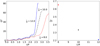 |
Fig. 20. Left panel: same as left panel of Fig. 17, but now the fixed parameters are ε = 0.1, l/R = 0.4, and ρi/ρe = 2.0, and we vary L/R = {8.0,10.0,12.0}. Right panel: estimated τKH as a function of the loop length. We note that in these panels time is normalized to the period of the internal torsional Alfvén wave, P = 2L/vA, i. |
5. Conclusions
We studied the nonlinear evolution of phase-mixed torsional Alfvén waves in a low-β coronal flux tube model with a constant axial magnetic field, which is line tied at the photosphere. This model consists of a tube with a uniform core, a transition layer where the density decreases continuously, and an external medium with uniform density.
The longitudinally fundamental mode of standing torsional Alfvén waves is excited at t = 0. First, the temporal evolution of the waves undergoes a quasi-linear phase that is well predicted by approximate analytical theory. Phase mixing evolves within the nonuniform layer by developing spatial oscillations of the azimuthal components of velocity and magnetic field that lead to the generation of smaller scales (see, e.g., Heyvaerts & Priest 1983). As a result, vorticity and current density increase in the system. In addition, the nonlinear coupling of Alfvén waves with slow magnetoacoustic waves through the ponderomotive force (see, e.g., Hollweg 1971) causes longitudinal flows.
Later in the evolution, the azimuthal shear flows generated by phase mixing trigger the KHi (Browning & Priest 1984). From that time onwards, the numerical results deviate significantly from those of quasi-linear analytic theory. Once the KHi is triggered, higher azimuthal wave numbers than the torsional mode appear in the system. As time increases, the KHi dramatically increases the total values of vorticity and current density and greatly enhances the development of small scales first initiated by phase mixing during the linear phase. The onset time of the KHi can be estimated from the evolution of the vorticity squared integrated over the whole computational box. Although this onset time depends on various model parameters, the KHi is typically triggered after few oscillation periods of the torsional waves. In particular, the parameter study showed that the wider the transition region, the later the KHi starts. Thus, a wide enough transition region can delay the onset and growth of KHi (see Terradas et al. 2018 for a similar result in the case of kink modes). In turn, the larger the velocity amplitude, the earlier the KHi is triggered because the system reaches the nonlinear regime faster. Regarding the density contrast, we find that for a small contrast, the higher the density contrast, the earlier the onset of the KHi. For sufficiently large contrasts, the onset time becomes roughly independent of this parameter. Finally, it is found that the longer the loop, the earlier the KHi is triggered relatively to the oscillation period of the torsional waves.
The KHi onset time estimated from the vorticity evolution always overestimates the critical times predicted analytically by Browning & Priest (1984). The reason for this discrepancy is that the critical time of Browning & Priest (1984) corresponds to the time at which the KHi is locally triggered within the nonuniform layer, while the onset time obtained from the vorticity evolution should be understood as a time for which the KHi has evolved enough to globally impact on the whole flux tube dynamics.
The development of the KHi drives the flux tube to a turbulent state. We find that the energy associated with the perturbations cascades with the perpendicular wavenumber following a −2 power law. Spatial scales much smaller than those generated by phase mixing alone are present during the turbulent phase. As a consequence, the effective Reynolds number decreases in the system much faster than what linear phase mixing predicts, meaning that the dissipative scales are approached much quicker (Terradas & Arregui 2018; Ebrahimi et al. 2020). Our ideal MHD simulations stop before such dissipative scales, which are reached in the corona. Those dissipative scales would eventually be reached at a later time, should turbulence continue to naturally evolve in the flux tube.
After turbulence has developed, the energy cascade to small scales speeds up considerably. Although the considered four-level AMR scheme is able to deal with those small scales during the initial stages of turbulence, it eventually fails to capture the fast generation of fine structures. We stopped our simulations precisely at that time to guarantee the physical validity of the results. For later times, numerical dissipation takes a predominant role and artificially affects the evolution. This highlights how crucial using sufficiently high spatial resolutions is to correctly resolve the fine dynamics associated with the nonlinear, turbulent evolution of the waves.
In connection with the recent results of Soler et al. (2021), the turbulent evolution of the torsional oscillations may provide a way to dissipate the large energy budget transmitted from the photosphere. Soler et al. (2021) conclude that wave energy dissipation is very inefficient in the linear regime. However, the turbulence discussed here may significantly enhance the heating rates (see, e.g., van Ballegooijen et al. 2011, 2017; Asgari-Targhi & van Ballegooijen 2012; Hillier et al. 2020). The results obtained here in this simple flux tube model open the door to more elaborate future studies. In the solar corona, where flux tubes are naturally inhomogeneous, this type of wave-mediated turbulence should occur, and there is much room to explore (see also Magyar et al. 2019). Additional effects to investigate could be, for instance, nonideal terms to study the actual energy dissipation, adding magnetic twist, and the evolution of torsional waves in curved coronal loops.
Movies
Movie associated with Fig. 5 (fig_5_rhovphithin) Access Supplementary Material
Movie associated with Fig. 6 (fig_6_rhovphithick) Access Supplementary Material
Movie associated with Fig. 7 (fig_7_vzrho) Access Supplementary Material
Movie associated with Fig. 8 (fig_8_currvortthin) Access Supplementary Material
Movie associated with Fig. 9 (fig_9_currvortthick) Access Supplementary Material
Acknowledgments
We acknowledge the support from grant AYA2017-85465-P (MINECO/AEI/FEDER, UE). S.D. acknowledges the support from the Spanish Ministry of Science and Innovation for the predoctoral FPI felloship PRE2018-084223. We thank Jaume Terradas for his technical assistance. We also thank the Universitat de les Illes Balears for the use of the Foner cluster. For the simulation data analysis we have used VisIT (Childs et al. 2012) and Python 3.5. In particular, we have used Matplotlib (Hunter 2007), Scipy (Virtanen et al. 2020), and Numpy (Harris et al. 2020). We are thankful to B. Vaidya and his contributors for the tool pyPLUTO. Finally, we thank Andrew Hillier, Tom Van Doorsselaere, and the anonymous referee for helpful comments.
References
- Alfvén, H. 1942, Nature, 150, 405 [NASA ADS] [CrossRef] [Google Scholar]
- Antolin, P., & Van Doorsselaere, T. 2019, Front. Phys., 7, 85 [Google Scholar]
- Antolin, P., Yokoyama, T., & Van Doorsselaere, T. 2014, ApJ, 787, L22 [NASA ADS] [CrossRef] [Google Scholar]
- Antolin, P., Okamoto, T. J., De Pontieu, B., et al. 2015, ApJ, 809, 72 [NASA ADS] [CrossRef] [Google Scholar]
- Arregui, I., Soler, R., Ballester, J. L., & Wright, A. N. 2011, A&A, 533, A60 [NASA ADS] [CrossRef] [EDP Sciences] [Google Scholar]
- Aschwanden, M. J., & Wang, T. 2020, ApJ, 891, 99 [Google Scholar]
- Asgari-Targhi, M., & van Ballegooijen, A. A. 2012, ApJ, 746, 81 [NASA ADS] [CrossRef] [Google Scholar]
- Ballester, J., Soler, R., Terradas, J., & Carbonell, M. 2020, A&A, 641, 17 [Google Scholar]
- Barbulescu, M., Ruderman, M. S., Van Doorsselaere, T., & Erdélyi, R. 2019, ApJ, 870, 108 [Google Scholar]
- Berger, T. E., Slater, G., Hurlburt, N., et al. 2010, ApJ, 716, 1288 [Google Scholar]
- Biskamp, D. 2003, Magnetohydrodynamic Turbulence (Cambridge: Cambridge University Press) [CrossRef] [Google Scholar]
- Bluteau, C. E., Jones, N. L., & Ivey, G. N. 2011, Limnol. Oceanogr. Methods, 9, 302 [Google Scholar]
- Browning, P. K., & Priest, E. R. 1984, A&A, 131, 283 [NASA ADS] [Google Scholar]
- Cargill, P., & de Moortel, I. 2011, Nature, 475, 463 [NASA ADS] [CrossRef] [Google Scholar]
- Chandrasekhar, S. 1961, Hydrodynamic and Hydromagnetic Stability (Oxford: Clarendon Press) [Google Scholar]
- Charbonneau, P., & MacGregor, K. B. 1995, ApJ, 454, 901 [NASA ADS] [CrossRef] [Google Scholar]
- Childs, H., Brugger, E., Whitlock, B., et al. 2012, High Performance Visualization-Enabling Extreme-Scale Scientific Insight, 357 [Google Scholar]
- Chorin, A. 1994, Vorticity and Turbulence, Applied Mathematical Sciences (Springer) [Google Scholar]
- Cooley, J. W., & Tukey, J. W. 1965, Math. Comput., 19, 297 [CrossRef] [MathSciNet] [Google Scholar]
- Cranmer, S. R. 2009, Liv. Rev. Sol. Phys., 6, 3 [Google Scholar]
- Cranmer, S. R., & van Ballegooijen, A. A. 2005, ApJS, 156, 265 [NASA ADS] [CrossRef] [Google Scholar]
- Dedner, A., Kemm, F., Kröner, D., et al. 2002, J. Comput, Phys., 175, 645 [Google Scholar]
- De Moortel, I., Hood, A. W., & Arber, T. D. 2000, A&A, 354, 334 [NASA ADS] [Google Scholar]
- De Moortel, I., McIntosh, S. W., Threlfall, J., Bethge, C., & Liu, J. 2014, ApJ, 782, L34 [Google Scholar]
- De Pontieu, B., McIntosh, S. W., Carlsson, M., et al. 2007, Science, 318, 1574 [Google Scholar]
- De Pontieu, B., Carlsson, M., Rouppe van der Voort, L. H. M., et al. 2012, ApJ, 752, L12 [NASA ADS] [CrossRef] [Google Scholar]
- De Pontieu, B., Rouppe van der Voort, L., McIntosh, S. W., et al. 2014, Science, 346, 1255732 [CrossRef] [Google Scholar]
- Ebrahimi, Z., Soler, R., & Karami, K. 2020, ApJ, 893, 157 [Google Scholar]
- Edwin, P. M., & Roberts, B. 1983, Sol. Phys., 88, 179 [Google Scholar]
- Fedun, V., Shelyag, S., Verth, G., Mathioudakis, M., & Erdélyi, R. 2011, Ann. Geophys., 29, 1029 [Google Scholar]
- Foullon, C., Verwichte, E., Nakariakov, V. M., Nykyri, K., & Farrugia, C. J. 2011, ApJ, 729, L8 [NASA ADS] [CrossRef] [Google Scholar]
- Frisch, U. 1995, Turbulence: The Legacy of A. N. Kolmogorov (Cambridge University Press) [Google Scholar]
- Galtier, S., Nazarenko, S. V., Newell, A. C., & Pouquet, A. 2000, J. Plasma Phys., 63, 447 [NASA ADS] [CrossRef] [Google Scholar]
- Goossens, M., Erdélyi, R., & Ruderman, M. S. 2011, Space Sci. Rev., 158, 289 [Google Scholar]
- Goossens, M., Andries, J., Soler, R., et al. 2012, ApJ, 753, 111 [Google Scholar]
- Guo, M., Van Doorsselaere, T., Karampelas, K., et al. 2019, ApJ, 870, 55 [NASA ADS] [CrossRef] [Google Scholar]
- Hahn, M., & Savin, D. W. 2014, ApJ, 795, 111 [NASA ADS] [CrossRef] [Google Scholar]
- Harris, C. R., Millman, K. J., van der Walt, S. J., et al. 2020, Nature, 585, 357 [CrossRef] [PubMed] [Google Scholar]
- Heyvaerts, J., & Priest, E. R. 1983, A&A, 117, 220 [NASA ADS] [Google Scholar]
- Hillier, A., & Polito, V. 2018, ApJ, 864, L10 [Google Scholar]
- Hillier, A., Barker, A., Arregui, I., & Latter, H. 2019, MNRAS, 482, 1143 [CrossRef] [Google Scholar]
- Hillier, A., Van Doorsselaere, T., & Karampelas, K. 2020, ApJ, 897, L13 [Google Scholar]
- Hollweg, J. V. 1971, J. Geophys. Res., 76, 5155 [NASA ADS] [CrossRef] [Google Scholar]
- Hollweg, J. V. 1978, Sol. Phys., 56, 305 [NASA ADS] [CrossRef] [Google Scholar]
- Hollweg, J. V. 1984, ApJ, 277, 392 [NASA ADS] [CrossRef] [Google Scholar]
- Howson, T. A., De Moortel, I., & Antolin, P. 2017, A&A, 607, A77 [NASA ADS] [CrossRef] [EDP Sciences] [Google Scholar]
- Howson, T. A., De Moortel, I., & Reid, J. 2020, A&A, 636, A40 [CrossRef] [EDP Sciences] [Google Scholar]
- Hunter, J. D. 2007, Comput. Sci. Eng., 9, 90 [NASA ADS] [CrossRef] [Google Scholar]
- Iroshnikov, P. S. 1964, Sov. Astron., 7, 566 [NASA ADS] [Google Scholar]
- Jafarzadeh, S., Solanki, S. K., Gafeira, R., et al. 2017, ApJS, 229, 9 [NASA ADS] [CrossRef] [Google Scholar]
- Jess, D. B., Mathioudakis, M., Erdélyi, R., et al. 2009, Science, 323, 1582 [NASA ADS] [CrossRef] [PubMed] [Google Scholar]
- Jess, D. B., Morton, R. J., Verth, G., et al. 2015, Space Sci. Rev., 190, 103 [Google Scholar]
- Karampelas, K., & Van Doorsselaere, T. 2018, A&A, 610, L9 [NASA ADS] [CrossRef] [EDP Sciences] [Google Scholar]
- Karampelas, K., Van Doorsselaere, T., & Antolin, P. 2017, A&A, 604, A130 [NASA ADS] [CrossRef] [EDP Sciences] [Google Scholar]
- Karampelas, K., Van Doorsselaere, T., & Guo, M. 2019, A&A, 623, A53 [NASA ADS] [CrossRef] [EDP Sciences] [Google Scholar]
- Kelly, R. E. 1965, J. Fluid Mech., 22, 547 [Google Scholar]
- Kohutova, P., Verwichte, E., & Froment, C. 2020, A&A, 633, L6 [NASA ADS] [CrossRef] [EDP Sciences] [Google Scholar]
- Kolmogorov, A. 1941, Akademiia Nauk SSSR Doklady, 30, 301 [Google Scholar]
- Kraichnan, R. H. 1965, Phys. Fluids, 8, 1385 [Google Scholar]
- Liu, J., McIntosh, S. W., De Moortel, I., Threlfall, J., & Bethge, C. 2014, ApJ, 797, 7 [NASA ADS] [CrossRef] [Google Scholar]
- Lohner, R. 1987, Comput. Methods Appl. Mech. Eng., 61, 323 [Google Scholar]
- Magyar, N., & Van Doorsselaere, T. 2016, A&A, 595, A81 [NASA ADS] [CrossRef] [EDP Sciences] [Google Scholar]
- Magyar, N., Van Doorsselaere, T., & Goossens, M. 2019, ApJ, 882, 50 [Google Scholar]
- Mann, I. R., Wright, A. N., & Cally, P. S. 1995, J. Geophys. Res., 100, 19441 [NASA ADS] [CrossRef] [Google Scholar]
- Martínez-Gómez, D., Soler, R., & Terradas, J. 2018, ApJ, 856, 16 [NASA ADS] [CrossRef] [Google Scholar]
- Mathioudakis, M., Jess, D. B., & Erdélyi, R. 2013, Space Sci. Rev., 175, 1 [NASA ADS] [CrossRef] [Google Scholar]
- Matsumoto, T., & Suzuki, T. K. 2012, ApJ, 749, 8 [NASA ADS] [CrossRef] [Google Scholar]
- Mignone, A., Bodo, G., Massaglia, S., et al. 2007, ApJS, 170, 228 [Google Scholar]
- Mignone, A., Zanni, C., Tzeferacos, P., et al. 2012, ApJS, 198, 7 [Google Scholar]
- Morton, R. J., Tomczyk, S., & Pinto, R. 2015, Nat. Commun., 6, 7813 [NASA ADS] [CrossRef] [Google Scholar]
- Mumford, S. J., Fedun, V., & Erdélyi, R. 2015, ApJ, 799, 6 [NASA ADS] [CrossRef] [Google Scholar]
- Nazarenko, S. 2011, Wave Turbulence, 825 (Berlin: Springer) [CrossRef] [Google Scholar]
- Ng, C. S., & Bhattacharjee, A. 1997, Phys. Plasmas, 4, 605 [NASA ADS] [CrossRef] [Google Scholar]
- Nocera, L., Priest, E. R., & Leroy, B. 1984, A&A, 133, 387 [Google Scholar]
- Ofman, L., & Thompson, B. J. 2011, ApJ, 734, L11 [NASA ADS] [CrossRef] [Google Scholar]
- Pagano, P., Pascoe, D. J., & De Moortel, I. 2018, A&A, 616, A125 [NASA ADS] [CrossRef] [EDP Sciences] [Google Scholar]
- Pope, S., Eccles, P., Pope, S., & Press, C. U. 2000, Turbulent Flows (Cambridge University Press) [CrossRef] [Google Scholar]
- Powell, K. G. 1994, An approximate Riemann solver for magnetohydrodynamics (that works more than one dimension), Tech. rep. [Google Scholar]
- Priest, E. R. 2012, Solar Magnetohydrodynamics (Springer Science& Business Media), 21 [Google Scholar]
- Prokopyszyn, A. P. K., Hood, A. W., & De Moortel, I. 2019, A&A, 624, A90 [NASA ADS] [CrossRef] [EDP Sciences] [Google Scholar]
- Rankin, R., Frycz, P., Tikhonchuk, V. T., & Samson, J. C. 1994, J. Geophys. Res., 99, 21291 [NASA ADS] [CrossRef] [Google Scholar]
- Roberts, B. 1973, J. Fluid Mech., 59, 65 [NASA ADS] [CrossRef] [Google Scholar]
- Roe, P. L. 1981, J. Comput. Phys., 43, 357 [Google Scholar]
- Ryutova, M., Berger, T., Frank, Z., Tarbell, T., & Title, A. 2010, Sol. Phys., 267, 75 [Google Scholar]
- Schekochihin, A. A., Nazarenko, S. V., & Yousef, T. A. 2012, Phys. Rev. E, 85 [CrossRef] [Google Scholar]
- Schnack, D. 2009, Lectures in Magnetohydrodynamics: With an Appendix on Extended MHD (Berlin Heidelberg: Springer) [Google Scholar]
- Shelyag, S., Fedun, V., Keenan, F. P., Erdélyi, R., & Mathioudakis, M. 2011, Ann. Geophys., 29, 883 [NASA ADS] [CrossRef] [Google Scholar]
- Shelyag, S., Mathioudakis, M., & Keenan, F. P. 2012, ApJ, 753, L22 [NASA ADS] [CrossRef] [Google Scholar]
- Shestov, S. V., Nakariakov, V. M., Ulyanov, A. S., Reva, A. A., & Kuzin, S. V. 2017, ApJ, 840, 64 [NASA ADS] [CrossRef] [Google Scholar]
- Shoda, M., Yokoyama, T., & Suzuki, T. K. 2018, ApJ, 853, 190 [NASA ADS] [CrossRef] [Google Scholar]
- Smith, P. D., Tsiklauri, D., & Ruderman, M. S. 2007, A&A, 475, 1111 [NASA ADS] [CrossRef] [EDP Sciences] [Google Scholar]
- Soler, R., & Terradas, J. 2015, ApJ, 803, 43 [NASA ADS] [CrossRef] [Google Scholar]
- Soler, R., Terradas, J., Oliver, R., Ballester, J. L., & Goossens, M. 2010, ApJ, 712, 875 [NASA ADS] [CrossRef] [Google Scholar]
- Soler, R., Terradas, J., Oliver, R., & Ballester, J. L. 2019, ApJ, 871, 3 [NASA ADS] [CrossRef] [Google Scholar]
- Soler, R., Terradas, J., Oliver, R., & Ballester, J. L. 2021, ApJ, 909, 190 [Google Scholar]
- Srivastava, A. K., & Dwivedi, B. N. 2017, JApA, 38, 61 [Google Scholar]
- Srivastava, A. K., Shetye, J., Murawski, K., et al. 2017, Sci. Rep., 7, 43147 [Google Scholar]
- Stix, M. 2012, The Sun an Introduction (Springer Science& Business Media) [Google Scholar]
- Terradas, J., & Arregui, I. 2018, Res. Notes Am. Astron. Soc., 2, 196 [Google Scholar]
- Terradas, J., & Ofman, L. 2004, ApJ, 610, 523 [NASA ADS] [CrossRef] [Google Scholar]
- Terradas, J., Oliver, R., & Ballester, J. L. 2006, ApJ, 642, 533 [NASA ADS] [CrossRef] [Google Scholar]
- Terradas, J., Andries, J., Goossens, M., et al. 2008, ApJ, 687, L115 [Google Scholar]
- Terradas, J., Magyar, N., & Van Doorsselaere, T. 2018, ApJ, 853, 35 [NASA ADS] [CrossRef] [Google Scholar]
- Tikhonchuk, V. T., Rankin, R., Frycz, P., & Samson, J. C. 1995, Phys. Plasmas, 2, 501 [NASA ADS] [CrossRef] [Google Scholar]
- van Ballegooijen, A. A., Asgari-Targhi, M., Cranmer, S. R., & DeLuca, E. E. 2011, ApJ, 736, 3 [Google Scholar]
- van Ballegooijen, A. A., Asgari-Targhi, M., & Voss, A. 2017, ApJ, 849, 46 [Google Scholar]
- Van Damme, H. J., De Moortel, I., Pagano, P., & Johnston, C. D. 2020, A&A, 635, A174 [CrossRef] [EDP Sciences] [Google Scholar]
- Virtanen, P., Gommers, R., Oliphant, T. E., et al. 2020, Nat. Methods, 17, 261 [Google Scholar]
- Wedemeyer-Böhm, S., Scullion, E., Steiner, O., et al. 2012, Nature, 486, 505 [NASA ADS] [CrossRef] [PubMed] [Google Scholar]
- Zaqarashvili, T. V. 2003, A&A, 399, L15 [NASA ADS] [CrossRef] [EDP Sciences] [Google Scholar]
- Zaqarashvili, T. V., Zhelyazkov, I., & Ofman, L. 2015, ApJ, 813, 123 [NASA ADS] [CrossRef] [Google Scholar]
All Figures
|
Fig. 1. Schema of the coronal flux tube model. The two gray planes located at the ends of the tube represent the solar photosphere where the magnetic field is anchored. |
| In the text | |
|
Fig. 2. Radial profiles of equilibrium Alfvén and sound speeds in a loop with l/R = 1 and ρi/ρe = 2. The values are normalized with respect to the external Alfvén speed. The vertical dashed lines denote the boundaries of the nonuniform layer. |
| In the text | |
|
Fig. 3. Azimuthal component of the velocity perturbation normalized with respect to the initial amplitude as a function of the radial position at various times. We used l/R = 1, ρi/ρe = 2, L/R = 10, and z = 0. Time is normalized as tvA, e/R. The vertical dashed lines denote the boundaries of the nonuniform layer. |
| In the text | |
|
Fig. 4. Vertical component of velocity perturbation, normalized as |
| In the text | |
|
Fig. 5. Top: cross-sectional cut of density at the tube center, z = 0, for the thin-layer case at three different simulation times indicated on top of each panel. Bottom: same cut, but for the azimuthal component of velocity. The full temporal evolution is available as an online movie. |
| In the text | |
|
Fig. 6. Same as Fig. 5, but for the thick-layer case. We note that the three selected simulation times are different from those of Fig. 5. The full temporal evolution is available as an online movie. |
| In the text | |
|
Fig. 7. Longitudinal cuts of density (top) and longitudinal component of velocity (bottom) at y = 0 for the thick-layer case at the same simulation times as in Fig. 6. The full temporal evolution is available as an online movie. |
| In the text | |
|
Fig. 8. Top: cross-sectional cut at z = 0 of vorticity squared (in logarithmic scale) for the thin-layer case at three different simulation times indicated above each panel. Bottom: same, but for the current density squared at z ≈ L/2. The straight lines seen in some panels are visualization artifacts at the boundaries of different AMR patches. These artifacts are not present in the actual simulation data. The full temporal evolution is available as an online movie. |
| In the text | |
|
Fig. 9. Same as Fig. 8, but for the thick-layer case. We note that the three selected simulation times are different from those of Fig. 8. The full temporal evolution is available as an online movie. |
| In the text | |
|
Fig. 10. Top: cross-sectional cut at z = 0 of vorticity squared (in logarithmic scale) for the thin-layer case at the final simulation time. The left and right panels correspond to the nonlinear numerical results and the linear analytic results, respectively. Bottom: same, but for the thick-layer case. |
| In the text | |
|
Fig. 11. Vorticity squared (top panel) and current density squared (bottom panel) integrated over the whole computational domain as a function of simulation time for both thin-layer (l/R = 0.4) and thick-layer (l/R = 1.5) cases. Red solid lines correspond to linear analytic results, and blue dashed lines correspond to nonlinear numerical results. Vorticity is normalized to the value at t = 0. No normalization is needed for current density since it vanishes at t = 0. |
| In the text | |
|
Fig. 12. Vorticity squared integrated over the whole computational domain as a function of simulation time for the thin-layer case. The various lines correspond to simulations with different levels of refinement in the AMR scheme: 1 (black dot-dashed line), 2 (brown dotted line), 3 (green dashed line), and 4 (blue solid line). For comparison purposes, the linear analytical value is also shown (red dashed line). Vorticity is normalized to the value at t = 0. |
| In the text | |
|
Fig. 13. Top panel: real part of the Fourier coefficients with p = 0, 1, 2, 3, 4, and 12 as functions of the computational time for an angular sampling of the azimuthal component of velocity at r = R and z = 0 in the thin-layer case. The two vertical dashed lines correspond to the critical time of Browning & Priest (1984), tcrit = 40, and the onset time inferred from the integrated vorticity slope change, τKH = 66. The linear analytic result, where only the p = 0 mode is present, is overplotted for comparison. Bottom panel: same as top panel but for the radial component of velocity. |
| In the text | |
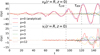 |
Fig. 14. Same as Fig. 13, but for the thick-layer case. Here, tcrit = 94 and τKH = 120. |
| In the text | |
|
Fig. 15. Amplitude spectrum (arbitrary units) of the averaged total energy of the perturbations for the thin-layer case at the end of the simulation for both numerical and linear analytic results. The vertical dot-dashed orange lines denote the maximum phase-mixing-generated wave number, kmaxR ≈ 105, obtained from Eq. (11), and an estimated wave number for which numerical diffusion starts to play a role, kdiffR ≈ 500. The red line is a least-squares linear fit for kmax < k⊥ < kdiff in log-log scale whose slope is −2.07 ± 0.02. The green line is the same fit but for k⊥ > kdiff, whose slope is −3.28 ± 0.07 |
| In the text | |
|
Fig. 16. Top: numerical (left) and analytic (right) effective Reynolds number in logarithmic scale at the end time of the simulation in the thin-layer case. These results are calculated in a cross-sectional cut at z = 0. The straight lines seen in the numerical result are visualization artifacts due to the AMR scheme. These artifacts are not present in the actual simulation data. Bottom: same as top panels, but for the thick-layer case. |
| In the text | |
|
Fig. 17. Left panel: vorticity squared integrated over the whole computational domain as a function of the simulation time for ε = 0.1, ρi/ρe = 2.0, L/R = 10, and l/R = {0.4,0.7,1.0,1.5}. The curves are normalized to the integrated vorticity squared at t = 0. Right panel: estimated τKH as a function of the width of the transition region, l/R. |
| In the text | |
|
Fig. 18. Left panel: same as left panel of Fig. 17, but now the fixed parameters are l/R = 0.4, L/R = 10, and ρi/ρe = 2.0, and we vary ε = {0.06,0.1,0.2,0.25}. Right panel: estimated τKH as a function of the amplitude of the velocity perturbation. |
| In the text | |
|
Fig. 19. Left panel: same as left panel of Fig. 17, but now the fixed parameters are ε = 0.1, L/R = 10, and ρi/ρe = 2.0, and we vary ρi/ρe = {2,5,6.5,10,13}. Right panel: estimated τKH as a function of the density contrast between the core of the flux tube and the external medium. |
| In the text | |
|
Fig. 20. Left panel: same as left panel of Fig. 17, but now the fixed parameters are ε = 0.1, l/R = 0.4, and ρi/ρe = 2.0, and we vary L/R = {8.0,10.0,12.0}. Right panel: estimated τKH as a function of the loop length. We note that in these panels time is normalized to the period of the internal torsional Alfvén wave, P = 2L/vA, i. |
| In the text | |
Current usage metrics show cumulative count of Article Views (full-text article views including HTML views, PDF and ePub downloads, according to the available data) and Abstracts Views on Vision4Press platform.
Data correspond to usage on the plateform after 2015. The current usage metrics is available 48-96 hours after online publication and is updated daily on week days.
Initial download of the metrics may take a while.