| Issue |
A&A
Volume 648, April 2021
|
|
|---|---|---|
| Article Number | A121 | |
| Number of page(s) | 11 | |
| Section | Interstellar and circumstellar matter | |
| DOI | https://doi.org/10.1051/0004-6361/202039746 | |
| Published online | 27 April 2021 | |
Testing the models of X-ray driven photoevaporation with accreting stars in the Orion Nebula Cluster★
1
Universitäts-Sternwarte, Ludwig-Maximilians-Universität München,
Scheinerstraße 1,
81679
München, Germany
e-mail: sflaisch@usm.lmu.de
2
European Southern Observatory, Karl-Schwarzschild-Straße 2,
85748
Garching bei München, Germany
Received:
23
October
2020
Accepted:
1
February
2021
Context. Recent works highlight the importance of stellar X-rays on the evolution of the circumstellar disks of young stellar objects, especially for disk photoevaporation.
Aims. A signature of this process may be seen in the so far tentatively observed dependence of stellar accretion rates on X-ray luminosities. According to models of X-ray driven photoevaporation, stars with higher X-ray luminosities should show lower accretion rates, on average, in a sample with similar masses and ages.
Methods. To this aim, we have analyzed X-ray properties of young stars in the Orion Nebula Cluster determined with Chandra during the COUP observation as well as accretion data obtained from the photometric catalog of the HST Treasury Program. With these data, we have performed a statistical analysis of the relation between X-ray activity and accretion rates using partial linear regression analysis.
Results. The initial anticorrelation found with a sample of 332 young stars is considerably weaker compared to previous studies. However, excluding flaring activity or limiting the X-ray luminosity to the soft band (0.5−2.0 keV) leads to a stronger anticorrelation, which is statistically more significant. Furthermore, we have found a weak positive correlation between the higher component of the plasma temperature gained in the X-ray spectral fitting and the accretion rates, indicating that the hardness of the X-ray spectra may influence the accretion process.
Conclusions. There is evidence for a weak anticorrelation, as predicted by theoretical models, suggesting that X-ray photoevaporation modulates the accretion rate through the inner disk at late stages of disk evolution, leading to a phase of photoevaporation-starved accretion.
Key words: protoplanetary disks / stars: pre-main sequence / planetary systems / stars: statistics / X-rays: stars
The data underlying Figs. 5 and A.1 are only available at the CDS via anonymous ftp to cdsarc.u-strasbg.fr (130.79.128.5) or via http://cdsarc.u-strasbg.fr/viz-bin/cat/J/A+A/648/A121
© ESO 2021
1 Introduction
The interaction between young stellar objects (YSOs) and their circumstellar disks is of fundamental importance for an understanding of planet formation and migration (e.g., Ercolano & Pascucci 2017). During their evolution, many YSOs are surrounded by circumstellar disks, from which material is accreted onto the protostar. This process is thought to be controlled by stellar magnetic field lines connecting the disk with the protostellar surface, leading to a complicated system of magnetic “accretion funnels” that channel the accretion flow (Hartmann et al. 2016). The infalling material generates shocks at the protostellar photosphere, giving rise to strong optical emission lines (in particular Hα) and optical and ultraviolet excess emission, from which the accretion luminosity Lacc can be inferred with spectroscopy (e.g., Alcalá et al. 2017) or photometry (e.g., Venuti et al. 2014). Together with the stellar parameters, the accretion rate Ṁacc can be obtained from Lacc via Ṁacc = LaccR∕(0.8 G M), where R and M are the stellar radius and mass, respectively, while the factor 0.8 originates from the assumption that the infall stems from the magnetically truncated disk with a typical radius of ~5 stellar radii (Hartmann et al. 2016).
Several observational studies support the expectation that the accretion rate is higher for more massive YSOs (e.g., Muzerolle et al. 2003; Natta et al. 2006; Telleschi et al. 2007; Manara et al. 2012; Alcalá et al. 2014, 2017). However, the observed spread of up to two orders of magnitude in accretion rates for stars with similar masses dilutes the Ṁacc−M relation (e.g., Hartmann et al. 2016; Manara et al. 2017; Alcalá et al. 2017). Since the disk material gets dispersed over time, the accretion rate also decreases with isochronal age (e.g., Hartmann et al. 1998). However, there is also evidence for stars with high accretion rates at old ages (e.g., Venuti et al. 2019).
The dispersal of the disk material is caused by strong disk winds. Observational evidence and simulations suggest that irradiation from the central star is an important driving mechanism of these disk winds (Alexander et al. 2014). In particular, models predict X-ray emission to be very efficient in photo-evaporating the circumstellar material (Ercolano et al. 2008a,b, 2009; Owen et al. 2010, 2011, 2012; Picogna et al. 2019; Wölfer et al. 2019), affecting the accretion rate (e.g., Drake et al. 2009) as well as planet formation and migration (e.g., Ercolano & Rosotti 2015; Ercolano & Pascucci 2017; Jennings et al. 2018; Monsch et al. 2019). Compared to main sequence stars, YSOs show highly elevated X-ray activity through all evolutionary stages (Feigelson & Montmerle 1999; Preibisch et al. 2005; Preibisch & Feigelson 2005). Observations (e.g., Preibisch et al. 2005; Telleschi et al. 2007) have shown that the X-ray luminosity of YSOs increases with increasing mass, analogously to the accretion rates.
The Chandra Orion Ultradeep Project (COUP) produced the largest available data set of X-ray emitting YSOs in a star forming region (Getman et al. 2005b). The analysis of these data showed that, on average, accreting YSOs have lower X-ray luminosities than non-accreting YSOs (Preibisch et al. 2005). Initial explanations for this observation were predominantly based on the notion that the accretion process suppresses, disrupts, or obscures the X-ray activity. While Güdel et al. (2007) suggested that the disks may be opaque for parts of the X-ray spectrum, Romanova et al. (2004) and Telleschi et al. (2007) proposed that the accretion process may change the coronal magnetic field structure or even strip off the coronal magnetic field (Jardine et al. 2006), leading to lower X-ray emission. Telleschi et al. (2007) also discussed the possibility that the accreted material may cool the coronal plasma and soften the X-ray emission, making it undetectable for charge-coupled device (CCD) X-ray detectors.
An alternative model introduced by Drake et al. (2009) and based on hydrostatic X-ray photoevaporation calculations suggests that the X-rays modulate the accretion flow according to the X-ray heated disk models from Ercolano et al. (2008a,b, 2009). The ionizing radiation from the central protostar heats up the gas in the surface layers of the disk. If the temperature exceeds the local escape temperature, the hot gas establishes a thermally driven wind and escapes from the disk. Far-ultraviolet (6 eV ≤ E < 13.6 eV) and soft X-ray (0.1 keV < E < 2 keV) radiation is expected to drive the strongest winds by heating up regions with H column densities on the order of 1021 cm−2 to 1022 cm−2. The mass loss associated with the winds interrupts the supply of material into the inner parts of the disk, which is still viscously accreting onto the star. After a few million years, the accretion rate has declined to values lower than the mass loss rate in the context of viscous accretion, and a gap forms in the disk. At this stage, erosion sets in and the accretion rate drops quickly. Stars with higher X-ray luminosities should arrive earlier at this stage and should therefore display lower accretion rates for a given age. A more detailed outline of the process is given in the review of Ercolano & Pascucci (2017).
In order to test this theory, several studies have been carried out: Drake et al. (2009) found an anticorrelation between the accretion rates and the mass-normalized X-ray luminosities in a sample of 44 young stars in the Orion Nebula Cluster (ONC). Previously, the Telleschi et al. (2007) study of 39 sources in the Taurus Molecular Cloud using data from the XMM-Newton Extended Survey pointed toward a similar relation. However, due to the small sample sizes, the results of these studies remained tentative. Bustamante et al. (2016) seemingly confirmed the results with a larger sample of 431 sources in the ONC.
Due to the importance of the Ṁacc−LX relation, we have performed a new analysis and checked the methods of Telleschi et al. (2007) and Bustamante et al. (2016) for possible biases. In particular, we have tested the hypothesis that young stars with similar masses and ages show lower accretion rates for higher X-ray luminosities, on average, using an unbiased partial regression analysis. Furthermore, we have tested how flaring activity may influence the Ṁacc−LX relation and studied the relation between the hardness of the X-ray spectrum and the accretion rates.
2 Sample data and selection
2.1 Source data
With a distance of ~403 pc (Kuhn et al. 2019) from our Sun, the ONC is one of the nearest regions of ongoing star formation (Bally 2008). The deepest and longest X-ray observation of a young stellar cluster in the history of X-ray astronomy is the COUP observation of the ONC with Chandra and the Advanced CCD Imaging Spectrometer (ACIS). An 838 ks exposure was made over a period of 13.2 days in January 2003, producing a data set of 1616 detected X-ray sources (Getman et al. 2005b). The fluxes for 1543 sources were obtained by integrating thermal plasma spectral fits. The total band luminosities for the 73 remaining, faintest, sources were estimated from the incident fluxes and the median energies. For our analysis, we used the total X-ray luminosity corrected for interstellar absorption (corresponding to the total 0.5–8.0 keV band).
Manara et al. (2012) determined accretion rates for 730 young stars with the photometric catalog from the HST Treasury Program (Robberto et al. 2013). They used the Wide Field and Planetary Camera 2 (WFPC2) observations carried out between October 2004 and April 2005 with the F336W (U), F439W (B), F656N (Hα), and F814W (I) filters. The photometric data were used to construct a U–B versus B–I color–color diagram. An isochrone representing the pure photometric emission without accretion was constructed using the synthetic BT-SETTL atmospheric model spectra from Allard et al. (2011), which were calibrated for the optical range. It was then assumed that the displacement of the observed sources from this isochrone is due to a combination of extinction and accretion. Using the Teff estimates from Da Rio et al. (2012), both AV and Lacc could be uniquely determined. With this procedure, the accretion luminosities for 271 sources were determined (the “U-excess sample”). These data were further used to obtain a relation between the accretion luminosities and the Hα luminosities, from which the remaining 459 accretion luminosities were derived (the “Hα sample”). This was possible because the emission in the hydrogen lines is linked to the accretion process (e.g., Hartmann et al. 2016).
For our analysis, we adopted the stellar masses determined by Manara et al. (2012) using the evolutionary models from Siess et al. (2000). However, we also repeated the analysis with the models from D’Antona & Mazzitelli (1994) and Palla & Stahler (1999) for comparison.
2.2 Crossmatching
The crossmatching between the two catalogs was performed with the match_xy routine of the tara-package1 as described in Broos et al. (2011). This routine uses the individual position uncertainties assuming a Gaussian distribution in order to determine a maximum acceptable distance such that ~ 99% of the counterparts in the two catalogs are identified as matches. The positional uncertainties for the X-ray sources were taken from the COUP table, and we assumed a positional uncertainty of 0.1′′ for the HST sources. The most significant match of each X-ray source is denoted the “primary match,” while less significant matches are labeled “secondary matches.” After this classification, the algorithm resolves many-to-one and one-to-many relations. Unambiguous one-to-one relationships are labeled “successful primary matches.” For our sample, this procedure led to 499 successful primary matches.
2.3 Gaia distances of the stars in the sample
From the 499 primary matches, 483 sources have parallaxes listed in the Gaia Early Data Release 3 (EDR3) catalog (Gaia Collaboration 2016, 2021). The mean parallax of the sources amounts to  , corresponding to a mean distance of ≈397.0 pc, which agrees with the distance of
  determined by Kuhn et al. (2019) using the earlier Gaia Data Release 2 (DR2).
We used the Gaia parallax data in order to identify stars that are likely not members of the ONC. In a first step, we selected candidates with a 5 −_ϖ parallax range that does not contain the mean distance. Next, we calculated the individual distances of the candidates. We defined candidates as foreground or background stars if their distances do not overlap, within 1σ, with the distance of the cluster determined by Kuhn et al. (2019). Using these criteria, we identified 11 targets in our sample that are most likely not members of the ONC: COUP 180 ( ), COUP 153 (
 ), COUP 1569 (
 ), COUP 518 (
 ), COUP 958 (
 ), COUP 1516 (
 ), COUP 173 (
 ), COUP 855 (
 ), COUP 1455 (
 ), COUP 847 (
 ), and COUP 1585 (
 ). These targets were removed from our sample, leaving a total of 488 sources.
In order to be consistent with the data from Manara et al. (2012), we scaled the X-ray luminosity to the distance of 414 pc (Menten et al. 2007). This does not affect our correlation analysis since the exact distance does not influence the slope of the relations.
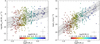 |
Fig. 1 Correlation of the mass accretion rate and the X-ray luminosity with the stellar mass. Left: mass accretion rate vs. stellar mass for young stars in the ONC. The accretion data and the masses are taken from Manara et al. (2012). The dashed line shows a single power-law fit for all objects with masses ≤ 2.0 M⊙. The solid line indicates the fitting result for the mass range 0.2 ≤ M ≤ 2.0, and the shaded region is its 1-σ deviation from the data. The cross indicates the typical uncertainty of the values. Right: same but for the X-ray luminosities taken from Getman et al. (2005a). The fitting parameters are listed in Table 2. |
2.4 Data selection
Following Drake et al. (2009), we set an upper mass limit of M = 2.0 M⊙. This reduced our sample to 453 sources. Like Manara et al. (2012), we further restricted the isochronal age interval according to 5.5 ≤ log(τ[yr]) ≤ 7.3 in order to reduce the amount of outliers in the Hertzsprung-Russell (HR) diagram in our sample. The final sample contains 446 sources.
2.5 Uncertainties of the quantities
The X-ray luminosities were derived from fitting spectral models, which are highly nonlinear (Preibisch et al. 2005). Following the authors, we assumed a typical uncertainty of 0.15 dex, based on the typical uncertainties derived from the spectral fits.
The accretion rates are subject to several uncertainties since they are calculated from values that are themselves subject to substantial uncertainties, such as the extinction and the stellar mass. We assumed typical uncertainties of 0.10 dex for the stellar masses and 0.42 dex for the accretion rates, as estimated by Alcalá et al. (2017) for YSOs in Lupus. The analysis of these authors suggests that the typical uncertainties are not substantially affected by the choice of the evolutionary models.
3 Correlation analysis
3.1 Relation between accretion rate, X-ray luminosity, and stellar mass
The left-hand side of Fig. 1 shows the (logarithmic) accretion rate as a function of the (logarithmic) stellar mass. In the first step, we followed the guideline of Isobe et al. (1990) and determined the slopes, β, of the regression line using different linear regression methods implemented in theInteractive Data Language (IDL) routine SIXLIN. We found values of 1.34 ± 0.14 (ordinary least squares [OLS]), 2.48 ± 0.15 (OLS bisector), 7.39 ± 0.80 (orthogonal reduced major axis), 3.27 ± 0.42 (reduced major axis), and 4.67 ± 0.39 (mean OLS). Since the slopes differ even within the range of their uncertainties, we conclude that the assumptions on which some of the methods are based are not fulfilled by our sample. Therefore, we determined the slopes using the fully Bayesian method from Kelly (2007), which takes the uncertainties of both variables into account. For this task, the IDL implementation LINMIX_ERR was used. The procedure yields a slope of 1.49 ± 0.16, which is consistent with the slope determined with the OLS method.
The dispersion of the regression line is 0.84 dex. This large scatter can be explained by measurement uncertainties and intrinsic variations. The slope agrees, within 1σ, with the value of 1.57 ± 0.23 that Bustamante et al. (2016) found for their Hα-sample, but it is lower than the value of 1.94 ± 0.23 that they found for their U-excess sample. The value agrees with the slope of 1.8 ± 0.2 that Alcalá et al. (2017) determined for Lupus and is at the lower end of the range of the typical findings of 1.5 to 3.1 from other studies (Hartmann et al. 2016).
When using the older tracks from D’Antona & Mazzitelli (1994), the slope becomes 1.77 ± 0.22, which is in agreement with the findings of other studies. In particular, this slope agrees with the value of 1.66 ± 0.07 that Ercolano (2014) found in their total sample, which also contains the accretion rates we used in our analysis. According to the authors, slopes of 1.45–1.70 are expected in the context of X-ray driven photo-evaporative disk dispersal.
However, newer studies of the Ṁacc − M relation provide evidence for a break in the distribution between M = 0.1 M⊙ and M = 0.3 M⊙. Manara et al. (2017) showed statistically that a double power law describes the Ṁacc −M relation slightly better than a single power law for a sample of accreting stars in Chamaeleon I. The slope is steeper for stars with masses lower than ~0.3 M⊙ and flatter for stars with higher masses. A similar behavior was found by Alcalá et al. (2017) for their sample in Lupus. They observed a steeper slope for stars with masses lower than 0.2 M⊙. Possible explanations provided by the authors are a faster evolution for objects with lower masses (Manara et al. 2012) or two different accretion regimes for different masses (Vorobyov & Basu 2009).
The distribution of our sample suggests a similar behavior: performing the linear regression using LINMIX_ERR only for objects with masses ≥0.2 M⊙ leads to the relation
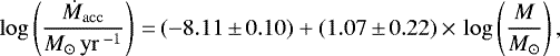 (1)
(1)
with a scatter of 0.80. The slope of 1.07 ± 0.22 is flatter compared to the fitting results for the full sample. Within 1σ, the slope agrees with the value of 1.37 ± 0.24 that Alcalá et al. (2017) found for objects with M ≥ 0.2 M⊙ in Lupus, but is steeper than the slope of 0.56 that Manara et al. (2017) found for M > 0.3 M⊙ in Chamaeleon I.
The right-hand side of Fig. 1 shows the X-ray luminosity as a function of the stellar mass. The dashed line represents the linear fitting result for the whole sample and has a slope of 2.29 ± 0.12, with a spread of 0.61. Limiting the mass range to values ≥0.2 M⊙ leads to a relation with a slightly flatter slope of 2.08 ± 0.16 and a spread of 0.58. The whole relation reads
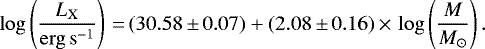 (2)
(2)
The slope is in agreement with the findings from Bustamante et al. (2016) of 1.90 ± 0.17 (Hα-sample), but higher than the value of 1.72 ± 0.17 (U-excess sample) and the value of 1.69 ± 0.11 found by Telleschi et al. (2007) for stars in the Taurus molecular cloud. Furthermore, the slope is larger than the value of 1.28 ± 0.07 found by Ercolano (2014) for their total sample and the 1.44 ± 0.10 obtained byPreibisch et al. (2005) despite the fact that they used the same evolutionary tracks. Repeating the analysis with the mass estimates listed in the COUP table, the slope becomes 1.67 ± 0.21, in agreement with the slope reported by Preibisch et al. (2005).
This indicates that the difference of the slopes is not caused by selection effects. In addition to the uncertainties in the Teff and Lbol values used to determine the masses in the HR diagram, there is also a bias that tends to overestimate the masses for brighter sources, resulting in a flattened relation between the masses and the X-ray luminosities. The bolometric luminosities used by Manara et al. (2012) were corrected for the accretion luminosities, which are particularly high for heavier stars. Furthermore, the ratio Lacc ∕(Lacc + Lbol) increases slightly with increasing mass (see Appendix C). Without this correction, the stellar luminosities are overestimated and the positions of the stars in the HR diagram are shifted toward tracks associated with higher masses. Since it is known that the X-ray luminosity is positively correlated with the bolometric luminosity (e.g., Preibisch et al. 2005), the masses of brighter X-ray sources are overestimated when the bolometric luminosity is not corrected for the accretion luminosity. It is possible that the LX − M relations found for other star forming regions may suffer the same effect.
Since low mass stars are intrinsically fainter, which gives rise to larger uncertainties, we limited further analysis to objects with masses ≥0.2 M⊙. Although this restriction reduces the sample size to 332, it avoids biases arising from the possible bi-model behavior of the Ṁacc − M relationship. Furthermore, this choice reduces the risk of a possible selection bias: The sample from Manara et al. (2012) is expected to be representative of the ONC stellar population down to ~0.1 M⊙. The COUP sample is thought to be complete down to ~0.2 M⊙ for lightly absorbed (AV < 5 mag) stars (Preibisch et al. 2005). We are therefore confident that our analysis will not be affected by a selection bias.
Sources from the U-excess sample make up 39% of our final sample, with sources from the Hα sample making up the remaining 61%. In order to quantitatively test the correlation between the parameters, we used the Spearman correlation coefficient, ρ, implemented in the IDL routine R_CORRELATE. It is 0.62 for the LX − M and 0.32 for the Ṁacc − M relation. The two-sided significance of its deviation from zero (the “p-value”) is < 0.001 for both cases, that is, the probability that the results are not due to a correlation is lower than 0.1%. The linear correlation coefficient, r, determined with LINMIX_ERR is 0.62 ± 0.04 and 0.32 ± 0.06, respectively.
It is worth noting that the slope of the LX − M relation is always higher than the slope of the Ṁacc − M relation in our sample, given the mass and isochronal age constraints of 0.2 M⊙≤ M ≤ 2.0 M⊙ and 5.5 ≤ log(τ∕yr) ≤ 7.3, not only for the evolutionary tracks from Siess et al. (2000) but also for the models from D’Antona & Mazzitelli (1994) and Palla & Stahler (1999). Depending on the chosen model, the slope of the LX −M relation is larger than the slope of the Ṁacc − M relation by factors of 1.6 − 2.0. Thus, a comparison of the connection between the slopes of the LX − M and the Ṁacc−M relations with current model predictions remains inconclusive with the current data set. A new theoretical investigation of the dependence of X-ray photoevaporation mass loss rates on stellar mass is in progress (Picogna et al., in prep.) and will address this point in more detail.
3.2 Relation between X-ray activity and accretion rate
The main goal of this work is to check the hypothesis that, in a sample with similar masses and ages, stars with higher X-ray luminosities show lower accretion rates on average. Since both LX and Ṁacc display a correlation with the stellar mass, one has to take their relation into account when analyzing the relation between LX and Ṁacc.
For thesake of readability, the following short notations are introduced: X stands for the logarithm of the X-ray luminosity, Y for the logarithm of the accretion rate, and m for the logarithm of the stellar mass. In order to illustrate the problem concerning the common mass dependence, a simple model consisting of two relations, X0 and Y0 – both of which are linearly dependent on a third variable, m – is regarded. Furthermore, scatter terms (sx and sy) are added. The scatter may be due to measurement uncertainties and/or the intrinsic variation of X0 and Y0 for identical m. The model is described by the following relations:

Here, X0 and Y0 are the relations one would ideally obtain from a linear regression of the X− m relation and the Y −m relation, respectively.
Since both X and Y depend on m, the X− Y relation will display a correlation, even if there is no intrinsic connection between the two quantities. The slope of this relation is d∕b, which can easily be shown. From Eqs. (5) and (6), it follows that
which is a line with a slope of d∕b. From this exercise, we can conclude that a correlation analysis will suffer spurious correlations if the parameters under consideration depend on a common additional variable, referred to as the “common response variable” in the literature (Shirley et al. 2010, for instance).
To overcome this problem, one usually resorts to a partial or semi-partial regression analysis (Wall & Jenkins 2003; Dey et al. 2019; Drake et al. 2009), which basically consists of two steps: First, the residua of one or more variables are calculated by taking the difference between the observed values and the linear regression solutions regarding the variables and the common response variable. Second, the correlation between the residua (partial correlation) or between the residua and the variables (semi-partial correlation) is investigated.
In our model, we know the linear regression solutions regarding m and can immediately state that the residua are X − X0 = sx and Y − Y0 = sy. Unlike the previous case, there is no shared variable in this approach.
A different method was used by Telleschi et al. (2007) and Bustamante et al. (2016) in their analysis of the relation between LX and Ṁacc. Applied to our model, the method works as follows: The first step is similar to the partial regression analysis; a linear regression on both X and Y with respect to m is performed, resulting in Eqs. (3) and (4). In the next step, the theoretical X as a function of Y if both relations only depend on m is constructed. From Eqs. (3) and (4) it follows that
 (7)
(7)
Next, the “residual X” is calculated as X − X0(Y). We note that Y, not Y0, is inserted into Eq. (7). Finally, a linear regression analysis is performed with the Y - [X − X0(Y)] relation. Telleschi et al. (2007) expected the values to scatter around a constant if [X − X0(Y)] is determined solely by the X - m and Y - m relations. However, this is not the case: from Eqs. (3) to (7) one obtains
 (8)
(8)
Since Y = Y0 + sy depends on sy as well, thismethod introduces a spurious correlation. Solving Eq. (8) for sy and inserting it into Eq. (6) provides
![\begin{equation*} Y[X - X_0(Y)]\,{=}\,c + d \cdot m - \frac{d}{b} \cdot ([X - X_0(Y)] - s_x), \end{equation*}](/articles/aa/full_html/2021/04/aa39746-20/aa39746-20-eq20.png)
implying that the relation will scatter around a line with a slope of − d∕b and not a constant. Since both b and d are positive in our case, this approach will inevitably introduce a bias toward an anticorrelation, even if there is no intrinsic connection between X and Y. In Appendix B, we demonstrate this with a synthetic data set. The approach would work if sy were negligible (in that case, the method is essentially equal to the semi-partial regression approach), but this is not the case: the scatter sy represents the scatter of the Ṁacc − M relation, which is particularly large, as shown in the previous section.
In order to avoid this kind of bias, we instead used the partial regression approach with the residual parameters LX ∕LX(M) and Ṁacc∕Ṁacc(M), where LX (M) and Ṁacc(M) are given by Eqs. (2) and (1). A scatter plot of the values is shown in the left panel of Fig. 2. We propagated the typical uncertainties to the residual values and performed the linear regression with the LINMIX_ERR routine. We found the following relation:
 (9)
(9)
Although the dispersion is large with 0.79 dex, a weak anticorrelation could be found (Spearman’s ρ is − 0.12 with p = 0.031 and a linear correlation coefficient ofr = −0.21 ± 0.07), indicating that, for similar masses, young stars with higher X-ray luminosities show lower accretion rates on average.
Furthermore, the choice of the evolutionary models used for the mass and isochronal age determination influences the result. When using the models from D’Antona & Mazzitelli (1994), the slope is − 0.21 ± 0.12 (ρ = −0.11, p = 0.082, and r = −0.17 ±, 0.09), while the models from Palla & Stahler (1999) lead to a slope of −0.34 ± 0.10 (ρ = −0.19, p = 0.001, and r = −0.28 ± 0.08).
In Fig. 2, the values are color coded according to the masses. A particular trend for different mass regimes is not visible.
The studies carried out by Telleschi et al. (2007) for the Taurus Molecular Cloud and by Bustamante et al. (2016) for the ONC also found an anticorrelation between accretion rates and X-ray activity. However, their results suggest a considerably stronger anticorrelation. As mentioned above, this is due to a bias introduced in the analysis method. Indeed, when using the partial regression method, the U-excess sample of Bustamante et al. (2016) displays no correlation at all, and the Hα-sample even shows a slight positive correlation. Combining the two samples and applying the same restrictions as described in Sect. 2.2 leads to the same weak anticorrelation as found in our analysis if we use the same evolutionary tracks from D’Antona & Mazzitelli (1994), as Bustamante et al. (2016) did.
3.3 Influence of the X-ray energy
Simulations suggest that X-ray photons in the soft band with E ≲ 2 keV are particularly efficient in driving disk winds (Ercolano & Pascucci 2017). Therefore, one would expect a stronger anticorrelation between the soft band (0.5−2.0 keV) X-ray luminosities, LX, soft, and the accretion rates. The LX, soft − M relation, as determined by the LINMIX_ERR method, has a flatter slope of 2.00 ± 0.16 and a spread of 0.58. The residual Ṁacc∕Ṁacc(M) − LX, soft∕LX, soft(M) relation shown on the right-hand side of Fig. 2 displays a slope of − 0.32 ± 0.10. With ρ = −0.14 (p = 0.008) and r = −0.25 ± 0.07, the anticorrelation is more significant. The p value is also below 5% for the models from D’Antona & Mazzitelli (1994) (p = 0.033) and Palla & Stahler (1999) (p < 0.001). The linear correlation coefficients are − 0.21 ± 0.09 and −0.31 ± 0.08, respectively.
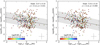 |
Fig. 2 Correlation of the residual mass accretion rate and the residual X-ray luminosity. Left: residual mass accretion rate as a function of residual X-ray luminosity. The regression line was obtained with the Bayesian LINMIX_ERR method, and the shaded region shows its 1σ scatter. The cross indicates the typical uncertainties. There is a weak anticorrelation. Right: residual mass accretion rate as a function of the residual soft band (0.5–2.0 keV) X-ray luminosity. The anticorrelation is stronger and more significant. |
3.4 Influence of flaring activity
In order to check whether flaring activity has an influence on the regression results, we tried to correct the X-ray luminosities from flaring influences. Wolk et al. (2005) identified periods of flaring from the light curves of the COUP sources and defined “characteristic count rates,” which represent the mean quiescent level of X-ray emission outside the time periods with significant flares. The ratio between this characteristic count rate and the mean count rate yields a correction factor, which can be used to determine a “characteristic” X-ray luminosity, LX, char.
The left-hand side of Fig. 3 shows the relation between LX, char and the stellar mass. It displays a significant positive correlation with ρ = 0.64 (p < 0.001) and r = 0.65 ± 0.04. The regression parameters of the LX, char−M relation differ only slightly from the respective values of the LX −M relation and match within their 1-σ uncertainties. With a spread of 0.55, the scatter is slightly smaller. Performing a similar partial regression analysis as the one in Sect. 3.2, but with the new relations, leads to
 (10)
(10)
with ρ = −0.16 (p = 0.004) and r = −0.26 ± 0.07. A scatter plot of the valuesis shown on the right-hand side of Fig. 3. The anticorrelation is stronger and more significant compared to the LX −Ṁacc relation. With a spread of 0.79, the scatter is similar to the corresponding relation without the flaring correction. Using the models from D’Antona & Mazzitelli (1994) for the mass and isochronal age estimates, the slope becomes − 0.32 ± 0.13 (ρ = −0.15, p = 0.017, and = − 0.23 ± 0.09), and the models from Palla & Stahler (1999) lead to a slope of − 0.44 ± 0.11 (ρ = −0.23, p < 0.001, and − 33 ± 0.07). The results suggest that strong flaring may partly disturb the anticorrelation between X-ray luminosity and accretion. The 3D magnetohydrodynamic simulations from Colombo et al. (2019) suggest that flaring activity is indeed able to promote or slow down accretion processes. From this scenario, it is expected that including flaring in the analysis will lead to an increased scatter, which tends to be higher for larger X-ray luminosities. This results in a flatter slope due to regression dilution.
3.5 Influence of stellar age
It is known that the X-ray luminosity decreases with isochronal age for similar masses (e.g., Preibisch & Feigelson 2005; Telleschi et al. 2007). A similar behavior can be observed for the accretion rates (e.g., Manara et al. 2012). We tried to remove the influence of the common isochronal age dependence from the Macc−LX relation. Forthis purpose, we regarded both the mass and the isochronal age simultaneously by fitting planes to the quantities. Uncertainties were not taken into account during this procedure. Scatter plots are shown in Fig. 5, and the regression parameters are listed in Table 1. Performing the partial regression analysis with these relations leads to a more significant anticorrelation:
 (11)
(11)
Spearman’s ρ is − 0.19 (p < 0.001), and the scatter is 0.74. The linear correlation coefficient is − 0.20 ± 0.05. Performing the analysis with the evolutionary tracks from D’Antona & Mazzitelli (1994) leads to a slope of − 0.37 ± 0.09 with ρ = −0.27 (p < 0.001), r = −0.26 ± 0.06, and a scatter of 0.73, while the tracks from Palla & Stahler (1999) yield a slope of −0.36 ± 0.08 with ρ = −0.26 (p < 0.001), r = −0.27 ± 0.06, and a scatter of 0.72. Thus, a significant anticorrelation is present for all three evolutionary models, with consistent slopes within 1σ. A scatter plot of the values is shown in Fig. 6.
In order to reduce the influence of the uncertainties in the individual stellar parameters, we repeated the analysis procedure using the accretion luminosity Lacc instead of Ṁacc. One obtains almost the same relation between the residual values:  . Plotting the residual accretion luminosity as a function of the residual accretion rate reveals that both quantities are almost identical, as seen in Fig. A.1. However, this result must be regarded critically due to the large uncertainties of the isochronal ages (e.g., Soderblom et al. 2014). Da Rio et al. (2014) suggest that the temporal decay of Macc may be overestimated due to a connection between the uncertainties of the mass accretion rates and the uncertainties of the isochronal ages.
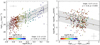 |
Fig. 3 Correlations using the “characteristic” X-ray luminosity LX, char. Left: LX, char vs. M. The cross indicates the typical uncertainties. The LX, char−M relation doesnot differ significantly from the LX−M relation (see Fig. 1). Right: same plot as in Fig. 2, but corrected for flaring activity, as described in Sect. 3.4. The anticorrelation is stronger and more significant. |
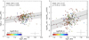 |
Fig. 4 Residual X-ray luminosity (left) and residual mass accretion rate (right) as a function of the higher plasma temperature, T2, gained in the two-component spectral fitting of Getman et al. (2005a). The cross indicates the typical uncertainties. A significant positive correlation is present in both cases. |
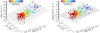 |
Fig. 5 3D plots of LX (left) and Ṁacc (right) with respect to both M and τ. The plots also show the best-fit surface described by the equation logY = A + B × logM + C × logτ, where Y stands for both LX and Ṁacc. The coefficients of the fits are listed in Table 1. The plot points are color coded according to the masses. |
Coefficients of the equation log Y = A + B × log M + C × log τ obtained by fitting LX, Ṁacc, and Lacc as a function of both M and τ using a standard Levenberg-Marquardt regression.
Summary of the correlation analysis results.
3.6 Relation between mass accretion rate and plasma temperature
The COUP X-ray spectra were fitted with a two-temperature thermal plasma model (Getman et al. 2005a). We investigated the relation between the higher temperature component, denoted as T2, and the residual X-ray luminosities and accretion rates. For the analysis, we rejected an obvious outlier with log (T2 [K]) > 8.
The results are summarized in Fig. 4 and Table 2. Both relations display a significant positive correlation, independently of the chosen evolutionary model. This result suggests that the hardness of X-ray spectra, which is associated with higher plasma temperatures, may influence the accretion rates in such a way that stars with harder X-ray spectra display higher accretion rates, on average, for a given mass and age. The development of new X-ray photoevaporation models, performed with spectra of different hardnesses, is in progress (Ercolano et al., in prep.). Since stars with harder X-ray spectra also have a higher X-ray luminosity on average, this effect counteracts the expected anticorrelation between X-ray luminosities and mass accretion rates. This mechanism may provide at least a partial explanation for the weakness of the observed anticorrelation, alongside the various uncertainties of the concerned parameters.
4 Summary and conclusions
We have presented a new analysis of X-ray luminosities of young stars in the ONC determined with Chandra as part of the COUP survey and with accretion data obtained from the photometric catalog of the HST Treasury Program. We have found a weak anticorrelation between residual X-ray luminosities and stellar accretion rates in a sample of 332 young stars. Since all relations analyzed in this work show a large scatter, a strong correlation could not be expected. Furthermore, it cannot be expected that the correlation becomes stronger using a larger sample. The nature of the large scatter is not fully understood. Apart from observational uncertainties, the stellar parameters are also plagued by intrinsic uncertainties due to the physical nature of young stars (see the discussion in Da Rio et al. (2014)). For instance, the X-ray luminosities likely suffer intrinsic differences in the X-ray activity levels of the YSOs (Preibisch et al. 2005). Both the X-ray luminosities and the accretion rates show a temporal variability that contributes to the observed scatter (e.g., Getman et al. 2005a; Venuti et al. 2015). A detailed analysis of the temporal variability of the accretion rates for the young stars in the ONC and its influence on the relation between X-ray emission and accretion is in progress (Flaischlen et. al, in prep.).
Our analysis showed that a stronger and more significant anticorrelation is obtained when the X-ray luminosity calculation is restricted to the soft X-ray regime (0.5−2.0 keV) or when strong flares are excluded. Taking the isochronal age dependence of the parameters into account, the anticorrelation is even more significant. Furthermore, we have found evidence that stars with harder X-ray spectra have higher X-ray luminosities and higher accretion rates on average. Both correlations are predicted by theoretical models of X-ray photoevaporation (Ercolano et al. 2008b, 2009, and in prep.; Owen et al. 2010; Picogna et al. 2019) and support the idea that protoplanetary disks undergo a phase of photoevaporation-starved accretion, as suggested by Drake et al. (2009).
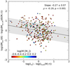 |
Fig. 6 Residual accretion rates vs. residual X-ray luminosities for the ONC taking both the mass and the isochronal age dependencesinto account. The anticorrelation is stronger and more significant. |
Acknowledgements
We wish to thank the referee for helpful suggestions. This work was funded by the Deutsche Forschungsgemeinschaft (DFG, German Research Foundation) in project PR 569/14-1 in the context of the Research Unit FOR 2634/1: “Planet Formation Witnesses and Probes: TRANSITION DISKS”. This project has received funding from the European Union’s Horizon 2020 research and innovation programme under the Marie Sklodowska-Curie grant agreement No 823823 (DUSTBUSTERS). This work has made use of data from the European Space Agency (ESA) mission Gaia (https://www.cosmos.esa.int/gaia), processed by the Gaia Data Processing and Analysis Consortium (DPAC, https://www.cosmos.esa.int/web/gaia/dpac/consortium). Funding for the DPAC has been provided by national institutions, in particular the institutions participating in the Gaia Multilateral Agreement. This research has used data obtained from the Chandra Data Archive and the Chandra Source Catalogue, and software provided by the Chandra X-ray Center (CXC) in the application packages CIAO and TARA. This research has also made use of the SIMBAD database and the VizieR catalog services operated at Strasbourg astronomical Data Center (CDS).
Appendix A Relation between the accretion luminosity and the stellar mass and isochronal age
The top part of Fig. A.1 shows a 3D plot of the accretion luminosity, Lacc, as a function of both the mass and the isochronal age. The parameters of the fitted plane are listed in Table 1. The bottom partof Fig. A.1 shows the residual mass accretion rate as a function of the residual accretion luminosity.
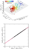 |
Fig. A.1 Correlations of the accretion luminosity Lacc. Top: 3D plotof Lacc with respect to both M and τ. The plot points are color coded according to the masses. Bottom: residual mass accretion rate as a function of the residual accretion luminosity. |
Appendix B Method used by Telleschi and Bustamante with a synthetic data set
In order to illustrate the issue with the method proposed by Telleschi et al. (2007) and described in Sect. 3.2, we tested the method with a simple model and a synthetic data set. A total of 332 logarithmic masses were generated randomly, and the values X0 and Y0 were calculated according to Eqs. (3) and (4), with the parameters a = 30.58 ± 0.07, b = 2.08 ± 0.16, c = −8.11 ± 0.10, and d = 1.07 ± 0.22. The standard deviations of sx and sy were distributed normally and chosen to be similar to the measured values of the ONC (0.58 for X0 and 0.80 for Y0). In this controlled model scenario, we know for sure that there is no intrinsic relation between X and Y. The top part of Fig. B.1 shows the result of the partial regression analysis. As expected, no correlation is indicated. The bottompart shows the result of the method used by Telleschi et al. (2007) and Bustamante et al. (2016) on the samedata set. One can clearly see an anticorrelation. The values scatter around a line with a slope of − d∕b and not around a constant. Spearman’s ρ suggests a strong anticorrelation as well. The color coding reveals a systematic shift in the Y direction that depends on m. We therefore recommend not using this method to study correlations.
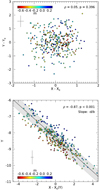 |
Fig. B.1 Correlations of the simulated data. Top: result of the partial regression analysis on a synthetic data set with 332 sources together with normally distributed scatter, which was chosen to be similar to the measured values. There is no correlation, as expected. Bottom: method used by Telleschi et al. (2007) and Bustamante et al. (2016) applied to the same data set. The values scatter around a line with a slope of − d∕b and not around a constant, as assumed by Telleschi et al. (2007). The reason is a common response variable, sy, introduced as an artifact of the analysis method as described in Sect. 3.2. |
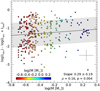 |
Fig. B.2 Ratio Lacc∕(Lacc + Lbol) as a function of the stellar mass. The cross indicates the typical uncertainties. There is a weak positive correlation. |
Appendix C Proportion of the accretion luminosity on the total luminosity
Figure B.2 shows the relation between the logarithmic mass and the logarithm of the ratio Lacc ∕(Lacc + Lbol). The typical uncertainty of Lacc was estimated to be 0.25 dex (Alcalá et al. 2017). We assumed a similar value for Lbol and propagated the error to the ratio. There is a weak positive correlation (ρ = 0.16, p = 0.004). A linear regression using the LINMIX_ERR routines yields a slope of 0.29 ± 0.19 and a linear correlation coefficient of 0.10 ± 0.07. The scatter amounts to 0.67. This result suggests that the proportion of the accretion luminosity on the total luminosity is higher for more massive stars on average. We note that this behavior also follows from the known Lacc −M and Lacc −L relations. Given that the latter is described by Lacc ∝ La and the former by Lacc ∝ Mb, the Lacc∕(Lacc + Lbol) − M relation steadily increases for a > 1 and b > 0.
References
- Alcalá, J. M., Natta, A., Manara, C. F., et al. 2014, A&A, 561, A2 [NASA ADS] [CrossRef] [EDP Sciences] [Google Scholar]
- Alcalá, J. M., Manara, C. F., Natta, A., et al. 2017, A&A, 600, A20 [NASA ADS] [CrossRef] [EDP Sciences] [Google Scholar]
- Alexander, R., Pascucci, I., Andrews, S., Armitage, P., & Cieza, L. 2014, in Protostars and Planets VI, ed. H. Beuther, R. S. Klessen, C. P. Dullemond, & T. Henning, 475 [Google Scholar]
- Allard, F., Homeier, D., & Freytag, B. 2011, in 448, 16th Cambridge Workshop on Cool Stars, Stellar Systems, and the Sun, eds. C. Johns-Krull, M. K. Browning, & A. A. West, ASP Conf. Ser., 91 [Google Scholar]
- Bally, J. 2008, in Handbook of Star Forming Regions, Vol. I, ed. B. Reipurth, Vol. 4 (Astronomical Society of the Pacific Monograph Publications), 459 [Google Scholar]
- Broos, P. S., Townsley, L. K., Feigelson, E. D., et al. 2011, ApJS, 194, 2 [Google Scholar]
- Bustamante, I., Merín, B., Bouy, H., et al. 2016, A&A, 587, A81 [Google Scholar]
- Colombo, S., Orlando, S., Peres, G., et al. 2019, A&A, 624, A50 [NASA ADS] [CrossRef] [EDP Sciences] [Google Scholar]
- D’Antona, F., & Mazzitelli, I. 1994, ApJS, 90, 467 [NASA ADS] [CrossRef] [Google Scholar]
- Da Rio, N., Robberto, M., Hillenbrand, L. A., Henning, T., & Stassun, K. G. 2012, ApJ, 748, 14 [Google Scholar]
- Da Rio, N., Jeffries, R. D., Manara, C. F., & Robberto, M. 2014, MNRAS, 439, 3308 [Google Scholar]
- Dey, B., Rosolowsky, E., Cao, Y., et al. 2019, MNRAS, 488, 1926 [Google Scholar]
- Drake, J. J., Ercolano, B., Flaccomio, E., & Micela, G. 2009, ApJ, 699, L35 [Google Scholar]
- Ercolano, B. 2014, Astron. Nachr., 335, 549 [Google Scholar]
- Ercolano, B., & Rosotti, G. 2015, MNRAS, 450, 3008 [NASA ADS] [CrossRef] [Google Scholar]
- Ercolano, B., & Pascucci, I. 2017, Roy. Soc. Open Sci., 4, 170114 [NASA ADS] [CrossRef] [Google Scholar]
- Ercolano, B., Drake, J. J., Raymond, J. C., & Clarke, C. C. 2008a, ApJ, 688, 398 [NASA ADS] [CrossRef] [Google Scholar]
- Ercolano, B., Young, P. R., Drake, J. J., & Raymond, J. C. 2008b, ApJS, 175, 534 [Google Scholar]
- Ercolano, B., Clarke, C. J., & Drake, J. J. 2009, ApJ, 699, 1639 [NASA ADS] [CrossRef] [Google Scholar]
- Feigelson, E. D., & Montmerle, T. 1999, ARA&A, 37, 363 [NASA ADS] [CrossRef] [Google Scholar]
- Gaia Collaboration (Prusti, T., et al.) 2016, A&A, 595, A1 [NASA ADS] [CrossRef] [EDP Sciences] [Google Scholar]
- Gaia Collaboration (Brown, A. G. A., et al.) 2021, A&A, in press, https://doi.org/10.1051/0004-6361/202039657 [Google Scholar]
- Getman, K. V., Feigelson, E. D., Grosso, N., et al. 2005a, ApJS, 160, 353 [Google Scholar]
- Getman, K. V., Flaccomio, E., Broos, P. S., et al. 2005b, ApJS, 160, 319 [Google Scholar]
- Güdel, M., Telleschi, A., Audard, M., et al. 2007, A&A, 468, 515 [NASA ADS] [CrossRef] [EDP Sciences] [Google Scholar]
- Hartmann, L., Calvet, N., Gullbring, E., & D’Alessio, P. 1998, ApJ, 495, 385 [NASA ADS] [CrossRef] [Google Scholar]
- Hartmann, L., Herczeg, G., & Calvet, N. 2016, ARA&A, 54, 135 [NASA ADS] [CrossRef] [Google Scholar]
- Isobe, T., Feigelson, E. D., Akritas, M. G., & Babu, G. J. 1990, ApJ, 364, 104 [Google Scholar]
- Jardine, M., Cameron, A. C., Donati, J.-F., Gregory, S. G., & Wood, K. 2006, MNRAS, 367, 917 [Google Scholar]
- Jennings, J., Ercolano, B., & Rosotti, G. P. 2018, MNRAS, 477, 4131 [NASA ADS] [CrossRef] [Google Scholar]
- Kelly, B. C. 2007, ApJ, 665, 1489 [Google Scholar]
- Kuhn, M. A., Hillenbrand, L. A., Sills, A., Feigelson, E. D., & Getman, K. V. 2019, ApJ, 870, 32 [Google Scholar]
- Manara, C. F., Robberto, M., Da Rio, N., et al. 2012, ApJ, 755, 154 [Google Scholar]
- Manara, C. F., Testi, L., Herczeg, G. J., et al. 2017, A&A, 604, A127 [NASA ADS] [CrossRef] [EDP Sciences] [Google Scholar]
- Menten, K. M., Reid, M. J., Forbrich, J., & Brunthaler, A. 2007, A&A, 474, 515 [NASA ADS] [CrossRef] [EDP Sciences] [Google Scholar]
- Monsch, K., Ercolano, B., Picogna, G., Preibisch, T., & Rau, M. M. 2019, MNRAS, 483, 3448 [NASA ADS] [CrossRef] [Google Scholar]
- Muzerolle, J., Hillenbrand, L., Calvet, N., Briceño, C., & Hartmann, L. 2003, ApJ, 592, 266 [Google Scholar]
- Natta, A., Testi, L., & Randich, S. 2006, A&A, 452, 245 [NASA ADS] [CrossRef] [EDP Sciences] [Google Scholar]
- Owen, J. E., Ercolano, B., Clarke, C. J., & Alexander, R. D. 2010, MNRAS, 401, 1415 [NASA ADS] [CrossRef] [Google Scholar]
- Owen, J. E., Ercolano, B., & Clarke, C. J. 2011, MNRAS, 412, 13 [NASA ADS] [CrossRef] [Google Scholar]
- Owen, J. E., Clarke, C. J., & Ercolano, B. 2012, MNRAS, 422, 1880 [NASA ADS] [CrossRef] [Google Scholar]
- Palla, F., & Stahler, S. W. 1999, ApJ, 525, 772 [Google Scholar]
- Picogna,G., Ercolano, B., Owen, J. E., & Weber, M. L. 2019, MNRAS, 487, 691 [Google Scholar]
- Preibisch, T., & Feigelson, E. D. 2005, ApJS, 160, 390 [Google Scholar]
- Preibisch, T., Kim, Y.-C., Favata, F., et al. 2005, ApJS, 160, 401 [Google Scholar]
- Robberto, M., Soderblom, D. R., Bergeron, E., et al. 2013, ApJS, 207, 10 [Google Scholar]
- Romanova, M. M., Ustyugova, G. V., Koldoba, A. V., & Lovelace, R. V. E. 2004, ApJ, 616, L151 [Google Scholar]
- Shirley, K. E., Small, D. S., Lynch, K. G., Maisto, S. A., & Oslin, D. W. 2010, Ann. Appl. Stat., 4, 366 [Google Scholar]
- Siess, L., Dufour, E., & Forestini, M. 2000, A&A, 358, 593 [Google Scholar]
- Soderblom, D. R., Hillenbrand, L. A., Jeffries, R. D., Mamajek, E. E., & Naylor, T. 2014, in Protostars and Planets VI, eds. H. Beuther, R. S. Klessen, C. P. Dullemond, & T. Henning, 219 [Google Scholar]
- Telleschi, A., Güdel, M., Briggs, K. R., Audard, M., & Palla, F. 2007, A&A, 468, 425 [Google Scholar]
- Venuti, L., Bouvier, J., Flaccomio, E., et al. 2014, A&A, 570, A82 [NASA ADS] [CrossRef] [EDP Sciences] [Google Scholar]
- Venuti, L., Bouvier, J., Irwin, J., et al. 2015, A&A, 581, A66 [NASA ADS] [CrossRef] [EDP Sciences] [Google Scholar]
- Venuti, L., Stelzer, B., Alcalá, J. M., et al. 2019, A&A, 632, A46 [CrossRef] [EDP Sciences] [Google Scholar]
- Vorobyov, E. I., & Basu, S. 2009, ApJ, 703, 922 [Google Scholar]
- Wall, J. V., & Jenkins, C. R. 2003, Practical Statistics for Astronomers, Cambridge Observing Handbooks for Research Astronomers (Cambridge University Press) [Google Scholar]
- Wölfer, L., Picogna, G., Ercolano, B., & van Dishoeck, E. F. 2019, MNRAS, 490, 5596 [CrossRef] [Google Scholar]
- Wolk, S. J., Harnden, F. R., J., Flaccomio, E., et al. 2005, ApJS, 160, 423 [Google Scholar]
All Tables
Coefficients of the equation log Y = A + B × log M + C × log τ obtained by fitting LX, Ṁacc, and Lacc as a function of both M and τ using a standard Levenberg-Marquardt regression.
All Figures
|
Fig. 1 Correlation of the mass accretion rate and the X-ray luminosity with the stellar mass. Left: mass accretion rate vs. stellar mass for young stars in the ONC. The accretion data and the masses are taken from Manara et al. (2012). The dashed line shows a single power-law fit for all objects with masses ≤ 2.0 M⊙. The solid line indicates the fitting result for the mass range 0.2 ≤ M ≤ 2.0, and the shaded region is its 1-σ deviation from the data. The cross indicates the typical uncertainty of the values. Right: same but for the X-ray luminosities taken from Getman et al. (2005a). The fitting parameters are listed in Table 2. |
| In the text | |
|
Fig. 2 Correlation of the residual mass accretion rate and the residual X-ray luminosity. Left: residual mass accretion rate as a function of residual X-ray luminosity. The regression line was obtained with the Bayesian LINMIX_ERR method, and the shaded region shows its 1σ scatter. The cross indicates the typical uncertainties. There is a weak anticorrelation. Right: residual mass accretion rate as a function of the residual soft band (0.5–2.0 keV) X-ray luminosity. The anticorrelation is stronger and more significant. |
| In the text | |
|
Fig. 3 Correlations using the “characteristic” X-ray luminosity LX, char. Left: LX, char vs. M. The cross indicates the typical uncertainties. The LX, char−M relation doesnot differ significantly from the LX−M relation (see Fig. 1). Right: same plot as in Fig. 2, but corrected for flaring activity, as described in Sect. 3.4. The anticorrelation is stronger and more significant. |
| In the text | |
|
Fig. 4 Residual X-ray luminosity (left) and residual mass accretion rate (right) as a function of the higher plasma temperature, T2, gained in the two-component spectral fitting of Getman et al. (2005a). The cross indicates the typical uncertainties. A significant positive correlation is present in both cases. |
| In the text | |
|
Fig. 5 3D plots of LX (left) and Ṁacc (right) with respect to both M and τ. The plots also show the best-fit surface described by the equation logY = A + B × logM + C × logτ, where Y stands for both LX and Ṁacc. The coefficients of the fits are listed in Table 1. The plot points are color coded according to the masses. |
| In the text | |
|
Fig. 6 Residual accretion rates vs. residual X-ray luminosities for the ONC taking both the mass and the isochronal age dependencesinto account. The anticorrelation is stronger and more significant. |
| In the text | |
|
Fig. A.1 Correlations of the accretion luminosity Lacc. Top: 3D plotof Lacc with respect to both M and τ. The plot points are color coded according to the masses. Bottom: residual mass accretion rate as a function of the residual accretion luminosity. |
| In the text | |
|
Fig. B.1 Correlations of the simulated data. Top: result of the partial regression analysis on a synthetic data set with 332 sources together with normally distributed scatter, which was chosen to be similar to the measured values. There is no correlation, as expected. Bottom: method used by Telleschi et al. (2007) and Bustamante et al. (2016) applied to the same data set. The values scatter around a line with a slope of − d∕b and not around a constant, as assumed by Telleschi et al. (2007). The reason is a common response variable, sy, introduced as an artifact of the analysis method as described in Sect. 3.2. |
| In the text | |
|
Fig. B.2 Ratio Lacc∕(Lacc + Lbol) as a function of the stellar mass. The cross indicates the typical uncertainties. There is a weak positive correlation. |
| In the text | |
Current usage metrics show cumulative count of Article Views (full-text article views including HTML views, PDF and ePub downloads, according to the available data) and Abstracts Views on Vision4Press platform.
Data correspond to usage on the plateform after 2015. The current usage metrics is available 48-96 hours after online publication and is updated daily on week days.
Initial download of the metrics may take a while.