| Issue |
A&A
Volume 648, April 2021
|
|
|---|---|---|
| Article Number | A18 | |
| Number of page(s) | 18 | |
| Section | Galactic structure, stellar clusters and populations | |
| DOI | https://doi.org/10.1051/0004-6361/202039192 | |
| Published online | 07 April 2021 | |
Infrared photometry and CaT spectroscopy of globular cluster M 28 (NGC 6626)⋆
1
Instituto de Astronomía, Universidad Católica del Norte, Av. Angamos 0610, Antofagasta, Chile
e-mail: This email address is being protected from spambots. You need JavaScript enabled to view it.
2
Millennium Institute of Astrophysics, Av. Vicuña Mackenna 4860, 782-0436 Macul, Santiago, Chile
3
Instituto de Astrofísica, Pontificia Universidad Católica de Chile, Av. Vicuña Mackenna 4860, 782-0436 Macul, Santiago, Chile
4
Instituto de Física-FCEN, Universidad de Antioquia, Calle 70 No. 52-21, Medellin, Colombia
5
Departamento de Astronomía, Universidad de Concepción, Casilla 160-C, Concepción, Chile
6
Dipartimento di Fisica e Astronomia, Universitá di Padova, Vicolo Osservatorio 3, 35122 Padova, Italy
7
Instituto de Física y Astronomía, Universidad de Valparaíso, Av. Gran Bretaña 1111, Playa Ancha, Casilla 5030, Chile
8
Gemini Observatory/NSF’s NOIRLab, 670 N. A‘ohoku Place, Hilo, HI 96720, USA
9
Space Telescope Science Institute, 3700 San Martin Drive, Baltimore, MD 21218, USA
10
Instituto de Investigación Multidisciplinario en Ciencia y Tecnología, Universidad de La Serena, Avenida Raúl Bitrán s/n, La Serena, Chile
11
Departamento de Física y Astronomía, Facultad de Ciencias, Universidad de La Serena, Av. Juan Cisternas 1200, La Serena, Chile
12
Departamento de Física, Facultad de Ciencias Exactas, Universidad Andres Bello, Av. Fernandez Concha 700, Las Condes, Santiago, Chile
13
Vatican Observatory, 00120 Vatican City State, Italy
Received:
15
August
2020
Accepted:
19
January
2021
Abstract
Context. Recent studies show that the inner Galactic regions host genuine bulge globular clusters, but also halo intruders, complex remnants of primordial building blocks, and objects likely accreted during major merging events.
Aims. In this study we focus on the properties of M 28, a very old and massive cluster currently located in the Galactic bulge.
Methods. We analysed wide-field infrared photometry collected by the VVV survey, VVV proper motions, and intermediate-resolution spectra in the calcium triplet range for 113 targets in the cluster area.
Results. Our results in general confirm previous estimates of the cluster properties available in the literature. We find no evidence of differences in metallicity between cluster stars, setting an upper limit of Δ[Fe/H] < 0.08 dex to any internal inhomogeneity. We confirm that M 28 is one of the oldest objects in the Galactic bulge (13–14 Gyr). From this result and the literature data, we find evidence of a weak age–metallicity relation among bulge globular clusters that suggests formation and chemical enrichment. In addition, wide-field density maps show that M 28 is tidally stressed and that it is losing mass into the general bulge field.
Conclusions. Our study indicates that M 28 is a genuine bulge globular cluster, but its very old age and its mass loss suggest that this cluster could be the remnant of a larger structure, possibly a primeval bulge building block.
Key words: Galaxy: bulge / globular clusters: individual: M28 / globular clusters: general
Based on observations gathered at the European Southern Observatory (programme ID 091.D-0535A), and with ESO-VISTA telescope (programme ID 172.B-2002).
© ESO 2021
1. Introduction
Our understanding of the complexity of Galactic globular clusters (GCs) has expanded impressively in the last decade after the discovery that they can host multiple stellar populations with different chemical enrichment histories (e.g., Piotto et al. 2015). The classical definition that they are simple stellar populations (i.e. initially chemically homogeneous aggregates of coeval stars) is now outdated. Carretta et al. (2009) showed that a certain degree of inhomogeneity of light chemical elements (C, N, O, Na, Mg, and Al) is observed in all GCs, and the only exception confirmed so far is Ruprecht 106 (Villanova et al. 2013), and possibly HP 1 (Barbuy et al. 2016). The coexistence of stars with different chemical compositions in the same cluster is believed to be due to the very early evolution of the system, where a second generation (or possibly more; e.g., Villanova et al. 2017) of stars formed from gas polluted by matter chemically processed by the first cluster stars. Intermediate-mass asymptotic giant branch stars (D’Antona et al. 2002), fast-rotating massive stars (Decressin et al. 2007), and massive binaries (de Mink et al. 2010) are the most accredited candidate polluters, but none of these self-enrichment scenarios is free of problems (see Renzini et al. 2015), and their origin is still hotly debated.
A spread in iron content is a characteristic restricted to only a few very massive globulars, such as ω Centauri (e.g., Piotto et al. 2005; Johnson et al. 2008) and M 54 (Carretta et al. 2010). In the self-enrichment model this is interpreted as the consequence of high initial cluster mass, enough to retain the highly accelerated ejecta of supernovae explosions (e.g., Lee et al. 2009). Ferraro et al. (2009) discovered the existence of two horizontal branches (HBs) in the bulge GC Terzan 5, a signature of the presence of two distinct stellar populations, with different spatial distributions, metallicities (Origlia et al. 2011), and possibly helium content (D’Antona et al. 2010) and/or ages (Ferraro et al. 2009). These peculiarities suggested that we might be witnessing the relic of a large building block of the Galactic inner spheroid (Lanzoni et al. 2010). Infrared data collected by the Vista Variables in the Vía Láctea (VVV) ESO public survey (Minniti et al. 2010) suggested a split HB even in NGC 6440 and NGC 6569 (Mauro et al. 2012). These two metal-rich GCs, as in Terzan 5, are among the 10 most massive of the 64 GCs within 4 kpc of the Galactic centre. More recent studies have excluded the presence of a significant metallicity spread in these clusters (Muñoz et al. 2017; Johnson et al. 2018). A spread in the content of heavy elements, however, is most likely present in M 22, another very massive GC lying in the inner regions of the Galaxy (Da Costa et al. 2009; Marino et al. 2009, 2011), although this too is still debated (Mucciarelli et al. 2015; Lee 2016).
Minniti (1995a) first suggested that there is a population of GCs that are associated with the Milky Way bulge, on the basis of metallicities, kinematics, and spatial distribution. M 28 (NGC 6626) is a poorly studied bulge GC located in the inner 3 kpc of the Galactic centre. In many aspects it is similar to the extensively analysed M 22, as it is also metal poor, is as massive as M 22 and NGC 6569 (Harris 1996; Peterson & Reed 1987), and shows a blue and extended HB. Still, it must be noted that it is more metal rich than M 22 by 0.4 dex (Villanova et al. 2017, hereafter V17), and Bica et al. (2016) classified it as a genuine bulge cluster, while they considered M 22 a likely Halo intruder. Few studies so far have estimated the age of M 28, but they all suggest that it should be a very old object (Testa et al. 2001; Roediger et al. 2014; Villanova et al. 2017; Kerber et al. 2018); indeed, it might be one of the oldest objects in the Galactic bulge.
The aforementioned peculiarities, and its similarity with M 22, make M 28 a good candidate cluster to search for an internal spread of iron. Prieto et al. (2012) analysed the properties of RR Lyrae variables in this cluster, and suggested the presence of multiple stellar populations to explain their peculiar hybrid Oosterhoff behaviour. Mauro et al. (2014, hereafter M14) re-analysed the calcium triplet (CaT) measurements of Rutledge et al. (1997, hereafter R97), and the resulting metallicity distribution appears wide, with possibly two peaks separated by ∼0.2 dex (see their Fig. 27). On the contrary, V17 claimed no intrinsic spread of metallicity among their 17 red giant branch (RGB) stars in M 28 because the observed measured dispersion of σ[Fe/H] = 0.06 dex equals the estimated errors.
In this work we investigate M 28 and its peculiarities further by means of VVV infrared photometry and low-resolution spectroscopy. In particular, our aim is to estimate the cluster age, and to analyse the possibility of an internal spread of iron via CaT spectroscopy of a large sample of stars.
2. Observations and data reduction
2.1. Photometric data
The infrared (IR) photometry of M 28 was performed on the data collected by the Vista Variables in the Vía Láctea survey (Minniti et al. 2010; Hempel et al. 2014). The data were acquired between 2010 July 1 and 2011 September 11 with the VIRCAM camera mounted on the VISTA 4m telescope at the Paranal Observatory (Emerson & Sutherland 2010), and reduced at the Cambridge Astronomical Survey Unit (CASU)1 with the VIRCAM pipeline (Irwin et al. 2004). During the observations the weather conditions fell within the survey’s constraints for seeing, airmass, and Moon distance (Minniti et al. 2010), and the quality of the data was satisfactory.
VIRCAM is an array of 16 independent 2048 × 2048 pixel detectors. We retrieved from the Vista Science Archive website2 the 175 frames collected by individual chips required to cover a wide field up to  from the cluster centre, in the three JHKs bands of the VVV survey. Each frame covered an area of approximately 10′ × 10′, and overlapped with contiguous images so that any point in the field was sampled by at least two frames. The retrieved data covered an area of ∼40′ × 30′ in Galactic longitude and latitude, respectively, with the cluster slightly off centre. The pixel scale was 0
 34, and the effective exposure time was 8s in the H and Ks bands, and 24s in J band (see Saito et al. 2012, for a more detailed description of the VVV data).
The PSF photometry was performed with the VVV-SkZ_pipeline (Mauro et al. 2013), based on the DAOPHOT II and ALLFRAME codes (Stetson 1994). The results were calibrated in the 2MASS astrometric and photometric system (Skrutskie et al. 2006), as detailed in Moni Bidin et al. (2011) and Chené et al. (2012). Between 45 and 55 2MASS stars were used in each frame for this process, with magnitudes in the range H = 9.8–11.8, J = 10.5–12.5, and Ks = 9.5–11.5. The VVV frames saturate at Ks≈12, but Mauro et al. (2013) showed that the PSF fit can recover correct magnitudes up to about two magnitudes above saturation. At brighter magnitudes, the completeness progressively declines. Cluster stars brighter than Ks = 8.5 are nevertheless so scarce, that we decided not to complement our VVV catalogue with the bright 2MASS sources present in the field. The trend of errors as a function of magnitude is shown in Fig. 1. The completeness of the VVV catalogue is limited by a lower detection rate in the J band, mainly because cluster stars are fainter in J than in the other bands, due to their red colour. Defining a successful detection only when the source is measured in all three bands, artificial star experiments on VVV frames showed us that our PSF photometry is complete at a level higher than 90% down to Ks≈17.5, although this is an average value because the completeness inevitably varies with crowding conditions in the wide area under study. The completeness rapidly fades at fainter magnitudes, dropping below 50% at Ks≈18.5.
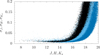 |
Fig. 1. Photometric errors as a function of magnitude in the J (blue), H (light blue), and Ks (black) bands. |
The density of the detected sources is shown in Fig. 2. In the figure the cluster field is mapped with 17″ × 17″ pixels, further smoothed with a 3 × 3 pixel boxcar. The map is relatively smooth, with a gentle gradient increasing with the negative Galactic latitude (i.e. the stellar density increases slightly toward the Galactic plane). The interstellar reddening is not constant in the field (see Sect. 3.6 and Fig. 10), but the stellar counts show no feature that can be caused by variations of extinction. On the contrary, they increase with it toward the Galactic plane. Hence, the stellar counts are negligibly affected by differential reddening.
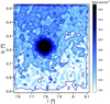 |
Fig. 2. Density map of the sources with Ks < 17.5 detected in the VVV frames. The density values in the blue-scale bar are in units of sources per arcmin2. The contour levels are shown at steps of 25 sources arcmin−2 from the minimum average background. |
2.2. Spectroscopic data
The spectra of 113 stars in the field of M 28 were collected in service mode with the ESO high-resolution multi-fibre spectrograph FLAMES/GIRAFFE (Pasquini et al. 2002) mounted on the VLT-UT2. The employed grating LR8 returned spectra in the range 8180–9365 Å, where the CaT spectral feature (a triplet of calcium lines at 8498, 8542, and 8662 Å) is found, with resolution R = 6500. All the spectra were collected with a single 900s exposure with one fibre configuration. The targets were selected by VVV photometry, to span the upper cluster RGB in the range Ks = 8.5–12. Priority was given to the stars in the inner cluster regions; however, due to fibre positioning limitations, objects up to  from the centre were observed. Their position in the cluster colour-magnitude diagram (CMD) is shown in Fig. 3, while the fibre IDs, coordinates, and photometric data are given in the first five columns of Table A.1.
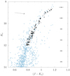 |
Fig. 3. Position of the spectroscopic targets in the VVV colour-magnitude diagram. The sources detected within 2′ of the cluster centre are overplotted in light blue. Solid dots, open symbols, and crosses indicate the stars classified as cluster members, additional member candidates, and field stars, respectively. Average errors as a function of magnitudes are plotted on the right, and the arrow shows the direction of interstellar reddening. |
The data were pre-reduced (bias-subtracted and flat-fielded), extracted, and wavelength-calibrated with the dedicated pipeline3. The wavelength calibration solution was based on the lamp spectra collected simultaneously during observations with five dedicated fibres. The spectra were extracted with an optimum algorithm (Horne 1986), and the average of 11 fibres allocated to the sky background was subtracted. The spectra were eventually normalised by fitting a low-order polynomial to the continuum, avoiding the three strong Ca II lines falling in the spectral range. The signal-to-noise ratio of the final spectra varied from ∼75 for the faintest targets (Ks≈12) to about 300 for the brightest objects (Ks≈8.6).
3. Infrared photometry
3.1. Radial density profile
Our analysis starts with the study of the spatial distribution of cluster stars because the definition of the cluster area in the wide field under analysis will often be needed throughout our work. Several studies have recently found that catalogue values of GC centres are typically discrepant by at least several arcseconds (e.g., Goldsbury et al. 2010; Watkins et al. 2015).
To determine the coordinates of the cluster centre, we calculated the average position of the stars within 3′ from the centre given by Noyola & Gebhardt (2006), and the result was used as input of a new iteration of the algorithm. The convergence was reached in three iterations, when the new centre differed from the input value by less than one pixel ( 34). We restricted the analysis to objects brighter than Ks = 16 to reduce the effects of incompleteness and the contamination of the Galactic background. The routine implicitly assumes that the field counts are homogeneous, else the result could drift from the cluster centre. However, the photometric cut of faintest sources (where the ratio of cluster to field stars is lowest) and the small area employed in the calculation prevented the small gradient seen in Fig. 2 from affecting the results. The centre was found at RA = 18:24:32.58, Dec = −24:52:13.6, less than 5″ from the definition of Noyola & Gebhardt (2006), and
  from that of Miocchi et al. (2013).
The centre previously defined was used to derive the radial density profile. To this end, we divided the area up to 13′ from the cluster centre in 180 annuli centred on it, with width  . We then calculated the density of the sources with Ks < 16.5 detected in each annulus. The result is shown in Fig. 4. The stellar counts rapidly decline outward to a constant value of ∼86 stars per arcmin2 at r > 11′, but they are hardly distinguishable from the field density already at r ∼ 4−5′. The star counts are severely affected by crowding in the central region, and the density stops increasing inward at
  . This incompleteness prevents us from studying the density profile in the inner area. Hence, we fit a King (1962) profile to the data at r > 2′, fixing the core radius
  from Trager et al. (1993). We verified that the results are insensitive to this assumption, mainly because our fit only deals with the outer regions and the bin width is narrower than rc itself. As a consequence, the results were unchanged when assuming alternative values from the literature (
 or
or  , Chun et al. 2015; Kerber et al. 2018). The best fit is shown in Fig. 4, and it returns
  . The fit curve also shows that the stellar counts start to be affected by incompleteness already at
  .
.
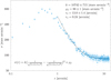 |
Fig. 4. Radial density profile of detected sources with Ks < 16. The curve shows the best-fit King profile in the range r = 2−13′. |
Previous measurements in the literature for M 28 report a tidal radius of  (Trager et al. 1993) and
  (Chun et al. 2015). Our result is slightly larger than theirs, but compatible within the errors. However, it must be considered that the non-uniform stellar background seen in Fig. 2, and the presence of the tidal structures discussed in Sect. 3.6, can easily lead to an overestimate of the tidal radius.
3.2. Decontaminated colour-magnitude diagram
Figure 4 shows that although the cluster occupies a large area in the sky, its density rapidly approaches the field background in the outer regions. For example, the annulus between r = 4′ and r = 5′ would statistically include about 400 cluster stars, but a field population six times larger. We therefore limit the cluster study to the area r < 4′ (hereafter defined as ‘cluster area’), to maximise the contrast between cluster stars and field contamination. The field contamination is relevant even in this area, where about 4300 field stars are expected out of a total of ∼9200 detections. Hence, we defined a field control area as an annulus centred on the cluster, with inner radius  and area equal to the cluster area. This region is still within the cluster tidal radius, but the expected cluster star density is so low in it that its effect on the following analysis is negligible.
We adopted a procedure similar to that used in Moni Bidin et al. (2011), based on the method of Gallart et al. (2003), to clean the CMD of the cluster area from the field contamination. The code scans the list of stars in the field area, and for each object it finds the star in the cluster area with the smallest distance d in the CMD, defined by
 (1)
(1)
where k is an arbitrary coefficient weighting a difference in colour with respect to a difference in Ks. A match is obtained when d is smaller than an arbitrary threshold dmax, and the star is removed from the catalogue of cluster sources. The parameters dmax and k involved in the process are, however, rather arbitrary. We fixed dmax = 0.3 magnitudes as in Gallart et al. (2003) and Moni Bidin et al. (2011); this choice revealed a good compromise between enough tolerance and the need to avoid associations between stars with very different photometry. Gallart et al. (2003) assumed k = 7 in their optical photometry, while Moni Bidin et al. (2011) extensively argued that in their VVV data a much smaller value (k = 1–2) was the preferable choice. We therefore experimented with small values, and eventually adopted k = 1 in our study.
The decontaminated CMD is shown in Fig. 5, superimposed on all sources from the cluster area. All the cluster sequences clearly emerge in the cleaned diagram, in particular the sub-giant (SGB) and asymptotic giant (AGB) branches, and a well-populated blue HB. Most of the field stars have been removed by the decontamination procedure, in particular the background RGB redder and fainter then the cluster sequence. A very slight residual contamination remains, observable in particular in correspondence to the field red clump and its upper main sequence (MS). This is most likely a consequence of the photometric incompleteness in the central cluster regions, which causes a small global under-detection of field stars. The few objects found between the cluster HB and RGB, however, could be (at least in part) cluster blue stragglers rather than field contaminants. This residual field contamination takes the shape of horizontal patterns in the faint red edge of the CMD, due to our choice of k = 1. This value implies that an offset in magnitude and in colour have the same weight in Eq. (1), but the circles of equal d become very elongated ellipses in a CMD that spans ten magnitudes in Ks and only one in (J − Ks).
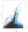 |
Fig. 5. Original (blue dots) and decontaminated (black dots) CMD of the cluster area (r < 4′). The arrow and the error bars are as in Fig. 3. The dotted line shows the saturation limit in VVV frames. |
Before the study of the decontaminated CMD, we felt it was worth analysing the differential reddening in the cluster field to check to what extent it can affect the results. To this end, we generated a series of artificial CMDs by means of Monte Carlo simulations, based on the cluster isochrone derived in Sect. 3.3 and the photometric errors as a function of magnitude shown in Fig. 1. The quantity of artificial stars at each magnitude was fixed to match the observed luminosity function of the decontaminated CMD to take into account observational effects such as the catalogue incompleteness in the inner regions. The results are shown in Fig. 6. The two panels look very similar, except for the aforementioned residual contamination in the observed diagram, and the presence of observed HB and AGB stars, not accounted for in the simulation. We calculated the width of the lower RGB in both the observed and synthetic diagrams in the magnitude interval Ks = 13.5−14.5, assuming the difference as being entirely due to differential reddening in the cluster area. For the observed CMD, a two-sigma clipping algorithm was applied to exclude from the calculation the cluster HB, and the residual contamination by the bulge MS seen on the redder side of the cluster RGB at this magnitude range. The observed sequence is slightly larger than the simulated one, and the quadratic difference of their widths indicates that the reddening variation is about ΔE(J − Ks) ≈ 0.024, equivalent to ΔE(B − V) ≈ 0.05. This value is in line with the reddening map shown in Fig. 10. This result shows that the differential reddening is small in the cluster field, and it will not be a major issue in the following analysis of the CMD.
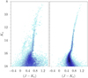 |
Fig. 6. Hess diagram of the decontaminated cluster CMD (left panel), and of a synthetic CMD calculated from the cluster isochrone and the photometric errors (right panel). |
3.3. Isochrone fit
We used the decontaminated CMD to derive the cluster reddening, distance, and age by means of isochrone fitting. We first defined the fiducial cluster sequence, with a fourth-order polynomial, fitting three sections of the CMD separately: the RGB (Ks< 15.5), the upper MS and turnoff region (Ks> 16), and the SGB intermediate between them. HB and AGB stars, along with the residual contamination from the field upper MS at about Ks≈15, (J − Ks) ≈ 0.55, were excluded from the fit to avoid spurious results. Nevertheless, the upper AGB merges with the RGB at its brightest end, and it was probably not fully removed. In addition, we applied a reduction algorithm in the turnoff and upper MS part to enhance the visibility of the cluster sequence and facilitate the fit. This consisted in dividing the data in random groups of ten stars of similar magnitude (ΔKs < 0.02), and substituting each group with a single point with its mean colour and magnitude. The results of this reduction algorithm, along with the fiducial cluster sequence, are shown in Fig. 7.
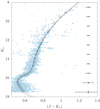 |
Fig. 7. Fiducial line of the cluster sequence (squares), and the best-fit DSED isochrones for τ = 12.5, 13.5, and 14.5 Gyr (dotted, full, and dashed curve, respectively). The decontaminated cluster CMD is shown as light blue points. |
We used the isochrones from the Dartmouth Stellar Evolutionary Database (DSED; Dotter et al. 2008) to derive the cluster parameters. We adopted a set of ages from τ = 11 to 15 Gyr in steps of 0.5 Gyr, with fixed values ![Mathematical equation: $ \left[ \frac{\mathrm{Fe}}{\mathrm{H}}\right]=-1.3 $](/articles/aa/full_html/2021/04/aa39192-20/aa39192-20-eq18.gif) and
and ![Mathematical equation: $ \left[ \frac{\mathrm{\alpha}}{\mathrm{Fe}}\right]=-0.4 $](/articles/aa/full_html/2021/04/aa39192-20/aa39192-20-eq19.gif) (V17). Testa et al. (2001) found evidence for a canonical helium abundance in M 28, and Kerber et al. (2018) showed that even a mild helium enhancement of ΔY = +0.05 is not compatible with the mean magnitude of its RR Lyrae stars. Hence, we adopted a normal helium abundance (Y = 0.2477) in our study.
(V17). Testa et al. (2001) found evidence for a canonical helium abundance in M 28, and Kerber et al. (2018) showed that even a mild helium enhancement of ΔY = +0.05 is not compatible with the mean magnitude of its RR Lyrae stars. Hence, we adopted a normal helium abundance (Y = 0.2477) in our study.
The SGB and lower RGB (Ks = 13–16) are the best-defined sequences in the diagram. Hence, we used them as references to adjust the cluster reddening E(J − Ks) and distance modulus (m − M)Ks for each isochrone independently, leaving the upper RGB and the turnoff region as diagnostics for τ. All the isochrones returned the same value of reddening E(J − Ks) = 0.20 ± 0.02, where the error was deduced by the width of the lower RGB, which is the dominant source of uncertainty when defining the fiducial cluster sequence and the best-fit isochrone. Assuming a standard reddening law and the absorption relations of Cardelli et al. (1989), this translates into E(B − V) = 0.38 ± 0.04. This result is slightly larger than the value E(B − V) = 0.35 or 0.36 given by the Schlegel et al. (1998) maps corrected as prescribed by Bonifacio et al. (2000) or Schlafly & Finkbeiner (2011), respectively, but it agrees with older literature estimates, which are in the range E(B − V) = 0.37−0.40 (Webbink 1985; Zinn 1985; Reed et al. 1988). More recent measurements preferred even higher values, E(B − V) = 0.42−0.44 (Davidge et al. 1996; Testa et al. 2001; Kerber et al. 2018). The assumption of a standard reddening law might be weak in this region of the sky, but we do not detect any systematic difference between the estimates based on IR photometry (Testa et al. 2001, and ours), and those based on optical data.
The best-fit distance modulus decreases with age, at the approximate pace of about 0.1 magnitudes per Gyr, from (m − M)Ks = 14.0 at τ = 10.5 Gyr to (m − M)Ks = 13.5 at τ = 14.5 Gyr. The best-fit isochrones for cluster age τ = 12.5, 13.5, and 14.5 Gyr are shown in Fig. 7. By construction, they all coincide on the lower RGB, where they were forced to match the cluster sequence to derive the best-fit reddening and distance modulus. They all fit the RGB rather well up to Ks = 12, but at brighter magnitude the results are uncertain due to the paucity of stars and the probable contamination of the derived cluster sequence by AGB objects. Some stars in the upper RGB, however, could be variable, which adds additional uncertainty to the fit of the brightest sequence. On the fainter end of the diagram (Ks > 15.5), on the other hand, the curves present different behaviours. Isochrones younger than 13 Gyr are definitely too blue on the main sequence, while the oldest solutions with τ ≥ 14 Gyr fail to reproduce the turnoff region at Ks ≈ 16. We therefore conclude that M 28 must be a very ancient object, with age in the range τ = 13–14 Gyr. This is older than the age found by Kerber et al. (2018) with the same DSED isochrones (12.1 ± 1.0 Gyr), although they found an older age (14.1 ± 1.0 Gyr) with BaSTI models (Pietrinferni et al. 2006). Within this age range, the distance modulus is constrained to (m − M)Ks = 13.6 ± 0.1, which translates into an absolute distance modulus of (m − M)0 = 13.5 ± 0.1, and a distance of d = 5.01 ± 0.23 kpc, assuming a standard reddening law to derive AKs from E(J − Ks). This assumption is safe in this case because AKs is small (of the order of 0.1 magnitudes), and any local deviations from the standard law produces a deviation one order of magnitude smaller than the error on (m − M)Ks. Our distance estimate is very similar to the recent result of Kerber et al. (2018, (m − M)0 = 13.51−13.67, depending on the isochrone set used), based on Hubble Space Telescope data.
3.4. Spectroscopic vs photometric stellar and cluster parameters
The spectroscopically derived temperature, gravity, and metallicity values of cluster members can be used to derive the cluster reddening and distance, avoiding the high degeneracy of multiple-parameter isochrone fits. Unfortunately, spectroscopic and photometric parameters often differ, and the differences strongly increase at low metallicity (see e.g., Sbordone et al. 2015, and references therein). Here we check the consistency of the spectroscopic measurements of V17 with those that can be derived from our IR photometry.
In Fig. 8 we compare the V17 results in the temperature-gravity plane with a DSED isochrone with τ = 13.5 Gyr and ![Mathematical equation: $ \left[ \frac{\mathrm{Fe}}{\mathrm{H}}\right]=-1.29 $](/articles/aa/full_html/2021/04/aa39192-20/aa39192-20-eq20.gif) (V17). The position of stars in this diagram is independent of reddening, distance, and age. We show only one isochrone in the figure because DSED curves with τ = 12.5, 13.5, 14.5 Gyr are totally indistinguishable in the plot. Figure 8 suggests a general agreement between the V17 and the DSED isochrones, but also the presence of a systematic, because the sample shows a drift to lower gravities at decreasing temperatures. This might be a consequence of deviations from local thermodynamic equilibrium (LTE), as non-LTE over-ionisation in the atmosphere of cool red giants can offset the spectroscopic gravities based on LTE ionisation equilibrium of iron lines (see e.g., Sitnova et al. 2015; Mashonkina et al. 2016).
(V17). The position of stars in this diagram is independent of reddening, distance, and age. We show only one isochrone in the figure because DSED curves with τ = 12.5, 13.5, 14.5 Gyr are totally indistinguishable in the plot. Figure 8 suggests a general agreement between the V17 and the DSED isochrones, but also the presence of a systematic, because the sample shows a drift to lower gravities at decreasing temperatures. This might be a consequence of deviations from local thermodynamic equilibrium (LTE), as non-LTE over-ionisation in the atmosphere of cool red giants can offset the spectroscopic gravities based on LTE ionisation equilibrium of iron lines (see e.g., Sitnova et al. 2015; Mashonkina et al. 2016).
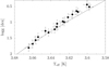 |
Fig. 8. Comparison between the V17 results (filled dots) and DSED isochrones (full curves), in the temperature-gravity plane. The errors shown are the internal uncertainties from V17. |
We transformed the spectroscopic effective temperature of the 17 targets of V17 into a theoretical colour (J − Ks)0 by means of the temperature-colour relation of Alonso et al. (1999). These relations are valid for (J − Ks) < 1, while the observed colour of our reddest targets is (J − Ks) ≈ 1.1. However, taking into account the reddening obtained in Sect. 3.3, their intrinsic colour is still within the range of validity of the Alonso et al. (1999) relations. The (J − K) colour in the TCS system used by Alonso et al. (1999) was transformed to the 2MASS system by means of the 2MASS4 and Alonso et al. (1998) equations. From the difference with the observed VVV colour, we obtained an estimate of the reddening for each star. The results span the range E(J − Ks) = 0.12−0.22, with average and standard deviation of E(J − Ks) = 0.17 ± 0.03. Under the assumption of a standard absorption law, this translates into E(B − V) = 0.33 ± 0.04. We do not see a clear gradient or pattern in the spatial distribution of E(B − V) of the 17 stars, but the average value of the western half of the sample is 0.03 magnitudes more reddened than the eastern half. This difference is negligible compared to the errors, but in line with the Schlegel et al. (1998) map that shows a tiny gradient of ΔE(B − V) = 0.02 increasing toward the west.
The spectroscopically derived reddening is lower than previous measurements in the literature, but still compatible within 1σ with our photometric estimate. To match our reddening estimate based on the isochrone fit, the V17 temperatures should be cooler by ∼80 K. A correction of all temperatures by this quantity would drift the observed points in Fig. 8 away from the theoretical isochrone, and an additional correction of gravities by +0.20 dex would be needed to recover the agreement in this plot. The errors quoted by V17 are smaller than these systematics by about a factor of two, but they represent only internal uncertainties.
If absolute magnitudes are derived from the isochrone assuming the V17 parameters, the distance modulus is overestimated by +0.8 magnitudes with respect to the value obtained from the isochrone fit (Sect. 3.3), and the resulting distance d ≈ 7.5 kpc is larger by 50%. We find that an offset of +160 K in temperature and +0.35 dex in gravity should be applied to the V17 measurements to force a match with isochrone fit reddening and distance modulus, while still keeping the agreement with the theoretical isochrone found in Fig. 8.
To further compare photometric and spectroscopic temperatures, we elaborated a method to estimate temperatures from photometric colours that can account for differential reddening and a non-standard reddening law. We therefore projected the position of the 17 V17 targets in the Two Colour Diagram (TCD) onto the same DSED isochrone used in Fig. 8 (τ = 13.5 Gyr and ![Mathematical equation: $ \left[ \frac{\mathrm{Fe}}{\mathrm{H}}\right]=-1.29 $](/articles/aa/full_html/2021/04/aa39192-20/aa39192-20-eq21.gif) ). We adopted the (J − Ks)−(Gbp − Ks) plane, where Gbp is the bluest Gaia band, because (G − Ks) is highly reddening-dependent while (J − Ks) is poorly affected by it. As a consequence, this combination returns an almost vertical reddening line, maximising its angle with the DSED isochrone and thus minimising the uncertainties of the projection procedure.
). We adopted the (J − Ks)−(Gbp − Ks) plane, where Gbp is the bluest Gaia band, because (G − Ks) is highly reddening-dependent while (J − Ks) is poorly affected by it. As a consequence, this combination returns an almost vertical reddening line, maximising its angle with the DSED isochrone and thus minimising the uncertainties of the projection procedure.
To avoid constraining the reddening law, we did not fix the slope of the reddening line in the TCD. Instead, we first corrected the (J − Ks) colours by the average cluster reddening E(J − Ks) = 0.20 previously determined, and connected each star to the point on the isochrone at its de-reddened (J − Ks)0. This calculation returned a different slope for each star; the values were then averaged to obtain our best estimate of the reddening line slope. This value was eventually kept fixed and used to project the targets onto the isochrone, and the intersection provided the photometric temperature and gravity of each star. This procedure thus assumes a unique (but not necessarily standard) reddening law, but it allows different reddening for each star because the length of the projection may vary from object to object.
We estimated the errors on the derived temperature and gravities calculating how these parameters were affected by the variation of one input quantity. We assumed a change of 1 Gyr and 0.05 dex respectively for age and metallicity, the VVV photometric errors for magnitudes and colours, our 1σ uncertainty for E(J − Ks); instead, for the slope of the reddening line we adopted the error-on-the-mean obtained during the estimate of this quantity. These uncertainties were then quadratically summed, obtaining an error of ∼100 K for Teff and ∼0.2 dex for log g.
The absolute magnitude in all bands can also be obtained from the projection on the isochrone. We thus derive E(J − Ks) = 0.20 ± 0.01 and (m − M)Ks = 13.5 ± 0.2 as the mean reddening and distance modulus for the 17 sample stars. These values perfectly match those obtained by means of the isochrone fit in the CMD (Sect. 3.3).
The photometric temperatures and gravities are systematically higher than the spectroscopic estimates of V17, with mean differences of ΔTeff = 167 ± 45 K and Δlog g = 0.39 ± 0.09. These values are essentially identical to those previously derived by comparison with cluster parameters derived from isochrone fit in the CMD. The standard deviation of the differences indicate that the external errors of the V17 measurements are approximately of the same order of magnitude as the uncertainties of our photometric estimates. In conclusion, the spectroscopic stellar parameters are much lower than the photometric values, and they lead to an underestimate of cluster reddening and a large overestimate of distance.
3.5. Proper motions
The temporal interval spanned by VVV observations is large enough to measure stellar proper motions (PMs). We used 76 VVV epochs acquired by the survey between 2010 and 2015, to derive the PM of all VVV sources within 6′ of the cluster centre. To this end, we employed the same procedure described in detail in Contreras Ramos et al. (2017), which returns values relative to the mean motion of bulge RGB stars in Galactic coordinates (μl, μb). Whenever needed during the analysis, we used the formulae from Poleski (2013) to transform  to the equatorial components
  , where
  and
and  . Our final catalogue comprised more than 64000 sources down to Ks ∼ 18.3.
The computed PMs show the presence of two populations: a wide distribution made up of bulge stars centred at  , as expected, and a small clump offset from the main distribution by ∼1–2 mas yr−1 in both coordinates. This is a clear signature of the different kinematics of the cluster with respect to the Galactic bulge. This conclusion is demonstrated in the vector point diagram (VPD; see Fig. 9), where we show the PM distribution of stars located along the cluster and field sequences observed in Fig. 5.
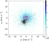 |
Fig. 9. VVV relative proper motions of stars in the cluster sequence (black dots), superimposed on the distribution of field stars. |
To derive the mean relative PM of the cluster, we performed a visual selection of cluster stars using both the CMD and the VPD. The procedure returned about 1000 likely members with Ks < 15 close (Δ(J − Ks) ≈ ± 0.02) to the cluster red RGB. After cleaning with a 2σ clipping algorithm to remove residual field contamination, we obtain the average cluster value of  mas yr−1. The quoted errors are the statistical errors-on-the-mean. To derive the absolute values, we matched the list of field RGB stars that have been used as reference stars to derive relative PMs with the Gaia DR2 database (Gaia Collaboration 2016, 2018a). We restricted the reference star sample to those stars showing relatively low PM errors (< 2 mas yr−1). After a 2σ clipping algorithm to clean the list from outlier measurements, the matched list comprised ∼400 objects. The comparison with Gaia measurements revealed a zero-point absolute offset of our relative PMs of
  mas yr−1. After applying this correction to the cluster value, the derived absolute PM for M 28 resulted
  mas yr−1 in equatorial components. Our result is in good agreement with the latest results of Gaia (Gaia Collaboration 2018b), and the later estimate of Vasiliev (2019), while there are some small differences with previous values from the literature, as shown in Table 1.
Literature estimates of the cluster proper motion.
3.6. Tidal structures
The wide field covered by VVV data is useful to study the possible presence of tidal structures around the cluster. To this end, we generated the density map of all stars with Ks < 17.5 located within Δ(J − Ks) = ± 0.05 from the best-fit isochrone defined in Sect. 3.3. This width was fixed to maximise the selection of cluster objects, taking into account photometric errors and the reddening variations in the wide 40′ × 30′ field under study. We also produced a similar map including all stars with Ks < 17.5 to study the behaviour of the general field. We then normalised both maps by the average stellar density calculated in the SW corner of the area, outside the cluster tidal radius where the field density has its minimum. Then, the normalised map of the general field was subtracted from the cluster map to remove the trend of the background field density.
The resulting map is shown in Fig. 10, normalised in units of the background noise, along with the Schlegel et al. (1998) reddening map of the same area. The cluster is actually doughnut-shaped in the map due to the decrease of completeness of our catalogue in the central regions (see Sect. 3.1 and Fig. 4), but this is not clear in the figure because the saturation limit of the colour scale was set at a lower level to observe the faint structures far from the centre. This also happened in Fig. 2 (compare the colour scale in Fig. 2 with the stellar counts in Fig. 4). Outside the inner dense regions, we detect a series of structures around the cluster. The most prominent feature is a long clumpy stripe in the direction opposite to the cluster motion. In addition, a tail extending toward the Galactic centre is also visible. A leading arm in the direction of the cluster motion is not found, while a reduced structure toward the Galactic anti-centre might be present, but more distant from the cluster centre than the other features. These structures do not follow the trend of the reddening map, nor the general gradient increasing with Galactic latitude observed in Fig. 2.
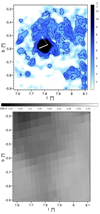 |
Fig. 10. Upper panel: normalised background-subtracted density map of the cluster area, in units of the background noise (σ). Contour levels are shown at 3σ, 4σ, and 5σ. The full white arrow shows the direction of the cluster proper motion, while the dashed arrow points toward the Galactic centre. Lower panel: Schlegel et al. (1998) reddening map of the same area as the upper panel. The reddening values in the greyscale bar are given in E(B − V). |
Kundu et al. (2019) studied RRLyrae extensions in 56 GCs, finding extra-tidal RR Lyrae in 20% of them, but they did not detect such stars in the area of M 28. However, Chun et al. (2012, 2015) claimed the detection of two tidal tails extending toward the Galactic centre and anti-centre, and a clumpy structure in the direction opposite to the cluster PM. All these structures are visible at a ∼2σ level in their maps (see Fig. 6 of Chun et al. 2015). Their work maps an area much larger than our, and the tail toward the Galactic anti-centre is clearly visible only beyond the cluster tidal radius. Our results closely reproduce theirs, confirming the existence of these tidal features.
4. CaT spectroscopy
4.1. Radial velocities
The radial velocity (RV) of target stars was measured cross-correlating (Simkin 1974; Tonry & Davis 1979) the three CaT lines with synthetic templates drawn from the library of Coelho et al. (2005) with [Fe/H] = −1.5, [α/Fe] = +0.4, and temperature and gravity varying with the position of the star on the cluster RGB. The cross-correlation was performed with the IRAF5 task fxcor. The measurements were reduced to heliocentric velocities, and the results are given in the sixth column of Table A.1. Our sample has five stars in common with V17, and the differences (in the sense ours−theirs) are small, within −2.1 and +0.2 km s−1. However, our RV is smaller than that of V17 for four of these five objects, and the mean difference is −0.8 km s−1, which suggests the presence of a tiny zero-point offset between the two measurement sets. This difference is of the order of our errors. We also have four targets in common with R97. The differences in this case are huge, with R97 RVs being higher by 20–40 km s−1. The average difference is +29 km s−1, which is similar to the difference between our estimate of the cluster RV and theirs (see Table 2).
Literature estimates of the cluster RV.
The RV distribution of all the targets is shown in Fig. 11 as a grey histogram. A peak at RV ≈ 10 km s−1 is evident, but the measurements are distributed in a wide range, indicating a relevant contamination by field stars. To reduce it and derive a more reliable cluster RV, we therefore analysed only the stars within r < 5′ of the centre, where the cluster dominates over the field density (see Fig. 4). The RV distribution of this sub-sample is shown in Fig. 11 as a black histogram. Only seven outliers with |RV|> 30 km s−1 are left, and they are all found at the faintest end of the magnitude distribution (Ks > 11). This is not surprising as the field contamination is expected to increase in the lower section of the RGB. We eventually obtained the cluster mean RV and dispersion fitting the probability plot (Hamaker 1978; Lutz & Hanson 1992) of this r < 5′ sample, excluding these six targets (see Moni Bidin et al. 2012, for more details on the fitting procedure). We thus find  km s−1 and σRV = 7.7 ± 0.5 km s−1, where the errors on these estimates was derived from the χ2 statistics of the fit. This value of the velocity dispersion is lower than but still consistent with the σRV = 9.4 ± 1.5 km s−1 found by V17. However, a unique definition of σRV from measurements of single stars is not straightforward because the velocity dispersion varies in a GC with distance from the centre, and the observed targets are distributed in a wide range of r. In Fig. 12 we show the variation in σRV with radial distance derived from our data. Our sample is not large enough to study the radial profile of the RV dispersion, but a decrease in σRV with r is clear. The trend derived by us is also very similar to the profile reported by Baumgardt et al. (2019)6, shown in the same figure for comparison. We find that the dispersion is roughly constant in the first 2′ from the centre, hence we limit the calculation to the targets with r < 2′, finding σRV, c = 8.4 ± 0.5 km s−1 for the central value. This result, which should still be regarded as a lower limit, matches the older estimate of Pryor & Meylan (1993), who proposed a central dispersion of 8.6 ± 1.3 km s−1. We therefore confirm that the internal velocity dispersion is high in M 28, indicating that this is a massive cluster.
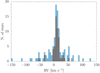 |
Fig. 11. Histogram of RV distribution of all spectroscopic targets (blue histogram), and targets within 4′ from the cluster centre (black histogram). |
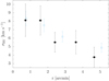 |
Fig. 12. Radial profile of the RV dispersion deduced from our sample. The big black dots are obtained binning our sample in steps of |

In the present analysis we have not accounted for the possible presence of binary stars, that could potentially affect the estimates of  and σRV. However, binaries are very rare in GC. According to the study of Lucatello et al. (2015), who found that the best estimate of the binary fraction among cluster RGB stars is ∼2%, less then one binary system should statistically be found in the sample of 21 stars with r < 2′. In addition, Bianchini et al. (2016) showed that the incidence of binaries on σRV is marginal, even when the binary fraction is high, because the velocity dispersion of the binary system sub-population is reduced by cluster dynamical effects.
Table 2 reports all the measurements of the cluster RV available in the literature. Previous results such as Rutledge et al. (1997) were very likely affected by high field contamination, while more recent estimates converge toward a similar value. Our result is slightly lower than the latest measurements by V17 and Gaia Collaboration (2018b).
4.2. Cluster membership
As discussed in Sect. 4.1, the spectroscopic sample is substantially contaminated by field stars, which must be removed to study the cluster metallicity distribution. Unfortunately, the PM information presented in Sect. 3.5 is not a useful tool in this context. Only 68 targets (∼60%) fell in the r < 6′ field covered by the PM catalogue. Moreover, all our targets are saturated in the VVV frames. While the VVV-SkZ_pipeline can recover an accurate photometry up to ≈3 magnitudes above the saturation level (Mauro et al. 2013), the astrometry is more sensitive to saturation, and our VVV PM catalogue misses 23 (∼34%) of the brightest remaining objects. In conclusion, we have PM estimates for only 45 targets (∼40%). In addition, the field-cluster separation in Fig. 9 is comparable to the error for single stars in most of the cases. Hence, we did not use the PM information to classify our targets, but we used it a posteriori to confirm the likelihood of our classification.
A first cleaning was performed inspecting the Na I doublet at 8195 Å, a feature very sensitive to stellar gravity and prominent in the spectra of dwarf stars (e.g., Collins et al. 2017). The 46 targets showing a very deep and strong doublet were classified as field dwarfs and excluded from further analysis. They are flagged as ‘dwarf’ in Table A.1.
Figure 11 shows that a combined selection on radial distance and RV can remove most of the residual contamination by field giants. To this end, we adopted a two-level selection, similar to that adopted by Salgado et al. (2013), where strict criteria are used to define the best cluster candidates, and looser criteria for an additional list of probable members. Considering that the cluster RV dispersion is 7.5 km s−1 (Sect. 4.1), and that at r ≈ 7′ the cluster density is already very close to the field level (Fig. 4), we first excluded from the analysis the 18 targets with either r > 7′ or |ΔRV|> 16 km s−1, where |ΔRV| is the difference between the target and cluster RVs. A flag was assigned to the remaining stars when r > 4′, and when |ΔRV|> 8 km s−1. Then, the 32 stars with no flag (r < 4′ and |ΔRV|< 8 km s−1) were selected as cluster members, those with two flags were excluded, and the 17 targets with one flag were considered as an additional set of lower-probability members. This selection criterion based solely on RVs and radial distance would have excluded all but three stars previously flagged as foreground dwarfs. Even these three surviving dwarfs (no. 49, 52, and 67) would have been classified only as possible members of lower probability.
In Fig. 13 we plot the VVV PM of the 45 targets for which this information is available, indicated with different symbols according to our classification. The PMs of all stars defined as cluster members or probable members are compatible with the cluster value, except for a group of targets at large negative  affected by large uncertainties. One object is found far from the cluster PM, and inside the 1σ ellipse of the field PM distribution. This star was removed from the CaT metallicity analysis. Foreground dwarfs and non-member red giants, on the contrary, are found prevalently at high positive
  far from the cluster value, and only two of them are potentially compatible with cluster membership. Hence, the PMs confirm that the results of our classification strategy are reliable. We also checked this classification with Gaia parallaxes. Among the stars classified as members or lower-probability members, we found only two targets whose parallaxes are incompatible with a distance of 5 kpc at ∼3σ level, while 30% of the objects classified as non-members do not survive this criterion. The two aforementioned stars were excluded from analysis.
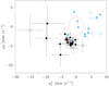 |
Fig. 13. Relative proper motion of the spectroscopic targets, according to our classification: dwarf stars and non-members (filled and empty blue dots), cluster members and probable cluster members (full and empty black dots). The large and small ellipses are centred on the cluster and field mean value, respectively, with semi-axis equal to the standard deviation of the distributions. |
4.3. CaT measurements
After RV measurements the spectra were shifted to laboratory wavelengths, and then we measured the equivalent widths (EWs) of the three CaT lines. The CaT feature is a powerful tool for estimating the metallicity of stars in clusters unreachable by high-resolution spectroscopy. However, as we show later, systematics can arise from differences in the procedure (e.g., continuum definition and normalisation, EW measurements). It would therefore not be safe to estimate the cluster metallicity from our measurements without a set of standard objects to correct for the systematics and to adjust the relation between our CaT indexes and the metallicity scale. Fortunately, the metallicity of M 28 metallicity has recently been measured from high-resolution spectra with accuracy (V17). Hence, here we focus only on star-to-star differences, which are independent from such calibration.
The spectral windows for the continuum definition on both sides of each line were taken from R97. The EWs were measured fitting each observed line with a Voigt profile in a broad band, namely 8490–8506 Å, 8532–8552 Å, and 8653–8671 Å. A variety of algorithms can be found in the literature to combine the three measurements into one value per star. Some authors prefer the direct sum of all the lines (e.g., Armandroff & Zinn 1988; Olszewski et al. 1991), while others use only the two strongest features (e.g., Armandroff & Da Costa 1991; Saviane et al. 2012), or a sum weighted with some specific values (R97). We experimented with these three alternatives, but identical results in terms of internal metallicity distribution were obtained in all the cases. Hence, hereafter we adopt the sum of the three lines (ΣEW) as the final value for each star, but this choice is irrelevant for our conclusions. The results are given in the eighth column of Table A.1. No measurement is given for the stars classified as dwarfs in Sect. 4.2. The EW of these objects was indeed largely discrepant, most of them returning a value more than 40% higher than the cluster average.
Our sample comprises four stars in common with R97. When we combine the EWs of the three Ca lines with the same weighted sum adopted in their work, and we compare the results, we find that the slope of our measurements to the R97 measurements is 0.96. However, our measurements are systematically higher, by 15% on average. The bands of line and continuum definition are the same in the two works, but R97 derived EWs by integration of the observed line profile instead of a fit, and this is likely the source of the difference. This is in line with the analysis of R97, who pointed out that there is a zero-point offset between the various methods to derive EWs, but the slopes are consistent with unity. Unfortunately, they do not directly analyse the case of a Voigt profile. Hence, as a consistency check, we repeated the measurements for these four stars with the same algorithm, but adopting a Gaussian function for the line fit. The resulting values were then corrected by means of the transformation formula proposed by R97. These measurements closely match those of R97, consistent within the errors with unit slope and zero offset.
The strength of the CaT lines depends on the evolutionary stage of the giant star as well as its metallicity. The value of ΣEW increases along the RGB, with a linear dependence on magnitude. This degeneracy must be removed to derive an estimate of metallicity for each individual star. To this end we followed the procedure of M14. We linearly fit the position of the 32 cluster stars in the ΣEW − ΔKs plane, where ΔKs = (Ks, HB − Ks), and Ks, HB is the magnitude of RGB at the HB level. We adopted Ks, HB = 13.0 from M14. We note that the intersection of HB and RGB is not visible in the cluster CMD (Cohen et al. 2017), but the exact value of Ks, HB is not relevant as long as we analyse the internal metallicity distribution. An incorrect definition of this parameter would only result in an identical zero-point offset for all the targets. We thus found the following solution (see Fig. 14):
 (2)
(2)
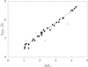 |
Fig. 14. Sum of the EW of the three CaT lines (ΣEW) of target stars, as a function of their magnitude difference with respect to the HB level (ΔKs). Full and empty dots are used for the cluster members and the additional possible cluster members, respectively. The line shows the linear fit of the cluster members. |
The slope is much steeper than that found by M14 combining the same VVV photometric data with spectroscopic measurements of Saviane et al. (2012, 0.385 Å mag−1), and R97 (0.348 Å mag−1). Part of this difference is due to the adopted algorithm for ΣEW because our direct sum of three EWs increases more with line strength then the sum of only two features (Saviane et al. 2012), or a weighted mean that reduces the contribution of some of them (R97). We verified that the slope reduces to ≈0.53 Å mag−1 if we adopt these algorithms for ΣEW. Another factor affecting the slope of the relation is the method used to measure EWs. When fitting the lines with a Gaussian profile, and correcting the results with the aforementioned equations given by R97, we found a slope of 0.387 Å mag−1, very similar to the result of M14.
The slope of Eq. (2) indicates how ΣEW grows with ΔKs at a fixed metallicity, while for a fixed ΔKs the value ΣEW depends on metallicity alone. To study the internal metallicity distribution of cluster stars, we therefore derived for each star the vertical distance from the cluster relation (Eq. (2)) in the ΣEW − ΔKs plane:
 (3)
(3)
We note that the star 66 is an outlier among cluster members at the fainter end of the sample, with ΔKs ≈ 1.4 and ΔΣEW < −250 mÅ7. This target was removed from the fit, and transferred to the group of possible additional cluster members in the following analysis. However, if this target is included, the zero-point and slope of Eq. (2) change by only 1σ (ΣEW = 5.872 + 0.656 × ΔKs).
The main source of uncertainty on ΔΣEW is the measurement error on the EWs of the three lines. To estimate it, we summed the spectra of the eight brightest targets with Ks < 9.1 (excluding those flagged as non-members or foreground dwarfs) to create a high-quality template spectrum. This was then multiplied by a linear function of random slope to alter its continuum, and degraded to S/N = 90, 170, and 250, to match the spectral quality of the observed spectra of the faintest, intermediate, and brightest targets, respectively. The same measurement routine was run on these artificial spectra as for the real data, and the procedure was repeated 100 times. The results showed a rms scatter decreasing with S/N, namely 45, 40, and 32 mÅ for the three cases, that was assumed as the measurement error on ΔΣEW. We also repeated the whole procedure adopting as a template a synthetic spectrum drawn from the Coelho et al. (2005) library, with Teff = 4250 K, log g = 1.5, ![Mathematical equation: $ \left[\frac{\mathrm{Fe}}{\mathrm{H}}\right]=-1.5 $](/articles/aa/full_html/2021/04/aa39192-20/aa39192-20-eq38.gif) , and
, and ![Mathematical equation: $ \left[\frac{\alpha}{\mathrm{Fe}}\right]=+0.4 $](/articles/aa/full_html/2021/04/aa39192-20/aa39192-20-eq39.gif) , and we found very similar results.
, and we found very similar results.
Another source of error on ΔΣEW are the uncertainties on the fit parameters in Eq. (2). We estimated these measuring how the dispersion of ΔΣEW varied when the parameters were altered by ±1σ. We found that it quadratically increased by 9 mÅ at all magnitude ranges. The photometric uncertainties on Ks are in the range 0.010–0.015 magnitudes, and they propagate into an error on ΔΣEW smoothly increasing with magnitude from 6 to 10 mÅ. Quadratically summing the measurement errors, and the uncertainties introduced by the fitting procedure and by photometric errors, we eventually obtained the final errors σΔΣ = 34, 42, and 47 mÅ in the bright, intermediate, and faint magnitude ranges, respectively.
4.4. Internal metallicity distribution
The global observed dispersion of ΔΣEW is σΔΣ, obs = 66 mÅ, comparable but slightly larger than the estimated errors σΔΣ. However, σΔΣ, obs = 11 mÅ for the five brightest stars with ΔKs > 4, much smaller than σΔΣ, while it slightly increases at fainter magnitudes from 71 mÅ for ΔKs = 2−4 to 74 mÅ for the ten faintest objects. If the measurements are scattered by an intrinsic spread, this should be of the order of  = 57 mÅ at all magnitudes fainter than ΔKs = 2.
The distribution histogram of ΔΣEW is shown in Fig. 15. The dark shaded area indicates a classical histogram in bins of 40 mÅ for the 32 stars considered cluster members, and the empty histogram is obtained including the 17 additional member candidates. The dotted line is the result of overlapping bins of the same width, in steps of 10 mA. The solid curve shows a continuous function obtained substituting to each star a Gaussian centred on the corresponding ΔΣEW, with width σ equal to the mean observational error (45 mÅ), and unit maximum height. One star classified as a cluster member and four lower-probability members are not shown in the figure because they are found at |ΔΣEW| > 200 mÅ, and they will not be considered further.
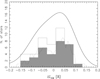 |
Fig. 15. Histogram of distribution of ΔΣEW for the observed targets. Different algorithms are shown, as detailed in the text. |
The histograms of Fig. 15 suggest a bimodal distribution, with two peaks at approximately ΔΣEW = ±50 mÅ, symmetric with respect to the mean cluster value (ΔΣEW = 0). Nevertheless, a series of independent tests agreed that this bimodality has no statistical significance. The Shapiro-Wink test (Shapiro & Wilk 1965) is considered one of the most powerful tools in the literature to test the normality of a distribution of small samples. The related Shapiro-Wink statistics for our 31 cluster members is W = 0.967, and it indicates that the data have a ∼47% probability of being normally distributed. This decreases to ∼33% if the 13 additional stars are included. The KMM algorithm8 (McLachlan & Basford 1988; Ashman et al. 1994) is somehow more optimistic, assigning the null hypothesis of a single Gaussian distribution a probability of 13% (20% when the 13 additional candidate members are included). KMM is a maximum-likelihood algorithm that assesses the improvement in fitting a multi-group model over a single-group model, and it has been repeatedly applied to astrophysical datasets (e.g., Ostrov et al. 1993; Lee & Geisler 1993; Bird 1994). A Kolmogorov-Smirnov test indicates that the ΣEW of the 31 members has a 55% probability of being drawn from a Gaussian distribution with σ = 66 mÅ, which increases to 75% if the additional member candidates are also considered. This suggests no significant statistical evidence of bimodality. In addition, if we compare the distributions with a Gaussian of width σ = 45 mÅ (equalling the estimated errors), the same probability is reduced but still acceptable (18% for the member stars, and 13% when the additional candidates are included). Hence, the test negates a statistical significance even to the observed dispersion ΔΣEW being wider than the estimated errors.
It would be very instructive to translate the values of ΔΣEW into ![Mathematical equation: $ \left[\frac{\mathrm{Fe}}{\mathrm{H}}\right] $](/articles/aa/full_html/2021/04/aa39192-20/aa39192-20-eq41.gif) , to estimate the errors, the possible internal spread, and the separation between the two peaks of a bimodal distribution, directly in a metallicity scale. However, we could not use ΔΣEW–
, to estimate the errors, the possible internal spread, and the separation between the two peaks of a bimodal distribution, directly in a metallicity scale. However, we could not use ΔΣEW–![Mathematical equation: $ \left[\frac{\mathrm{Fe}}{\mathrm{H}}\right] $](/articles/aa/full_html/2021/04/aa39192-20/aa39192-20-eq42.gif) calibrations from the literature (e.g., M14) because our EW measurements are not on the same scale of the previous works, as shown in Sect. 4.3. We obtained a rough metallicity scale for our measurements from the stars in common with R97. We first derived a metallicity value for each of them by means of the M14 calibration; then we used them to fit a linear relation between
calibrations from the literature (e.g., M14) because our EW measurements are not on the same scale of the previous works, as shown in Sect. 4.3. We obtained a rough metallicity scale for our measurements from the stars in common with R97. We first derived a metallicity value for each of them by means of the M14 calibration; then we used them to fit a linear relation between ![Mathematical equation: $ \left[\frac{\mathrm{Fe}}{\mathrm{H}}\right] $](/articles/aa/full_html/2021/04/aa39192-20/aa39192-20-eq43.gif) and our ΔΣEW values. The fit indicates that ΔΣEW = 100 mÅ corresponds to about
and our ΔΣEW values. The fit indicates that ΔΣEW = 100 mÅ corresponds to about ![Mathematical equation: $ \Delta\left[\frac{\mathrm{Fe}}{\mathrm{H}}\right]\approx0.15 $](/articles/aa/full_html/2021/04/aa39192-20/aa39192-20-eq44.gif) dex. This rough result is reasonable, as it indicates that our estimate of the observational errors (∼45 mÅ) equals ≈0.07 dex in metallicity, which is closely comparable with the accuracy expected by M14 for relative CaT measurements. According to this scale the two peaks observed in Fig. 15 would be separated by ≈0.13–0.14 dex, and the spread of 57 mÅ enhancing the observed distribution compared to the estimated errors would be about 0.08 dex.
dex. This rough result is reasonable, as it indicates that our estimate of the observational errors (∼45 mÅ) equals ≈0.07 dex in metallicity, which is closely comparable with the accuracy expected by M14 for relative CaT measurements. According to this scale the two peaks observed in Fig. 15 would be separated by ≈0.13–0.14 dex, and the spread of 57 mÅ enhancing the observed distribution compared to the estimated errors would be about 0.08 dex.
5. Discussion
5.1. Dynamical mass
The large velocity dispersion found in Sect. 4.1 is in line with the high cluster total luminosity. In Fig. 16, we show the central RV dispersion and the absolute integrated magnitude in the V band for all the Galactic GCs for which these estimates are available. All data were drawn from the Harris (1996) catalogue, except for M 28, where we compare our RV dispersion with the average of the available absolute magnitude estimates (Webbink 1985; Peterson & Reed 1987; van den Bergh et al. 1991). The plot shows that our result closely fits the σRV − MV relation for Galactic GCs. However, we note that our estimate should still be regarded as a lower limit for the central value because it is obtained for stars distributed in the inner 2′ from the centre.
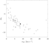 |
Fig. 16. Absolute luminosity in the V band as a function of the central RV dispersion of all GCs in the Harris (1996) catalogue with available measurements. The black dot represents M 28, with our dispersion measurement. |
The large velocity dispersion suggests that M 28 should be a massive cluster. To confirm this we estimated its dynamical mass from the King (1966) model, as modified by Illingworth (1976, Eq. (9)), assuming  , d = 5.01 ± 0.23 kpc, and σRV, c = 8.4 ± 0.5 km s−1 from this work, and
  from the literature (see Sect. 3.1). The model parameter μ was calculated from the tidal and core radii as in Illingworth & Illingworth (1976). We thus find
  . Alternatively, we find
  from the de Vaucouleurs (1959) model (Illingworth 1976, Eq. (13)), with the half-light radius re = 2.25 ± 0.37 pc (van den Bergh et al. 1991).
Mandushev et al. (1991) showed that the simplified single-mass King model at the basis of our estimate should underestimate  by about 0.3 dex with respect to more elaborated multi-component King models. It should be noted that if we applied this offset to our result, our two independent estimates would actually coincide. Very interestingly, our value based on this single-mass King model is very similar to the result obtained by Mandushev et al. (1991) with the same method, while the higher value returned by the de Vaucouleurs model matches the more recent estimate of Baumgardt & Hilker (2018) based on more elaborated N-body simulations.
We do not correct our result obtained from the King model for the expected underestimate, but we do assume the weighted average of our two results as our best estimate for the cluster mass,  , which is intermediate between the results of Mandushev et al. (1991) and Baumgardt & Hilker (2018). According to these two compilations, this value classifies M 28 as one of the 30% most massive systems among the 147 catalogued Galactic GCs.
5.2. Bulge age-metallicity relation
Our analysis of VVV photometry indicates that M 28 is a very old cluster, indeed one of the oldest objects in the Galactic bulge, as previously suggested in the literature (Testa et al. 2001; Roediger et al. 2014; Villanova et al. 2017; Kerber et al. 2018). On the other hand, while some metal-poor halo intruders can be found in the inner Galactic regions (e.g., Myeong et al. 2019), M 28 is also one of the most metal-poor objects catalogued as a genuine bulge GC by Bica et al. (2016). To put this result into context, in Fig. 17 we compare the age and metallicity estimates available in the literature for bulge GCs. We included NGC 6569 as a genuine bulge cluster, although Bica et al. (2016) classify it as an ‘outer shell’ object, while we excluded Terzan 5, because its complex stellar population suggests that its origin is probably distinct from that of the other objects in the sample (Lanzoni et al. 2010). For metallicity, we based our value on the most recent high-resolution spectroscopic measurements whenever possible, namely for HP1 (Barbuy et al. 2016), M 28 (V17), NGC 6522 (Barbuy et al. 2009), NGC 6528 (Muñoz et al. 2018), NGC 6558 (Barbuy et al. 2007), and NGC 6569 (Johnson et al. 2018). For all other objects (NGC 6304, NGC 6553, NGC 6624, NGC 6637, NGC 6652, NGC 6717, NGC 6723), we relied on the compilation of Carretta et al. (2009). The main reference for age estimates were Dotter et al. (2010, NGC 6304, NGC 6624, NGC 6637, NGC 6717, and NGC 6723) and VandenBerg et al. (2013, NGC 6304, NGC 6624, NGC 6637, NGC 6652, NGC 6717, NGC 6723), plus additional measurements for single clusters, namely HP1 (Kerber et al. 2019), NGC 6522 (Meissner & Weiss 2006; Barbuy et al. 2009; Kerber et al. 2018), NGC 6528 (Calamida et al. 2014; Feltzing & Johnson 2002; Momany et al. 2003; Lagioia et al. 2014), NGC 6553 (Zoccali et al. 2001), NGC 6558 (Barbuy et al. 2007), NGC 6569 (Saracino et al. 2019), and NGC 6624 (Saracino et al. 2016). When more than one measurement is available, in Fig. 17 we show the mean value, with the error-on-the-mean as an associated uncertainty.
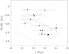 |
Fig. 17. Age-metallicity relation of bulge clusters. The dashed line indicates the linear fit of the data, while the dotted line shows a similar relation for halo objects. Empty light blue dots are used for the single literature measurements, while full black dots show the average value for each cluster. The outlier NGC 6553 is shown as a triangle, while M 28 is shown as a larger diamond. |
Figure 17 shows that an age-metallicity relation (AMR) is most likely present among bulge GCs: all objects with [Fe/H] ≲ −0.8 are older than ∼12.5 Gyr, while all but one of the more metal-rich GCs are younger than ∼12.0 Gyr. The only exception to this general trend is NGC 6553, which is one of the oldest (13 ± 1 Gyr) and most metal-rich ([Fe/H] = −0.16 ± 0.06) clusters in the sample. The AMR is clear but not well defined, because the objects span a rather narrow range in age, and the age measurements are affected by large errors. These uncertainties also blur the intrinsic dispersion that might indicate the degree of inhomogeneity in the chemical composition at early epochs. While metallicities are in general accurately measured by high-resolution spectroscopic studies, the use of different model isochrones introduces systematics in the age estimates (see e.g., Kerber et al. 2018), and a homogeneous determination for all the objects would be required. Even so, we observe that as the bulk of the age determinations come from a handful of works with many objects in common, the systematics between them tend to cancel out. An AMR is observable in Fig. 17 even if it considers only the single measurements instead of averages, although with an increased dispersion.
In Fig. 17 the AMR of the Galactic halo GCs is also shown for comparison. This was obtained with a linear fit of age and metallicities from the VandenBerg et al. (2013) compilation, considering objects classified as halo members by Leaman et al. (2013), and excluding members of the Sagittarius galaxy (e.g., Mottini & Wallerstein 2008). The comparison shows that the bulge GC system clearly formed and evolved extremely fast. At the earliest stages, 13–14 Gyr ago, it formed clusters 5–10 times more metal rich than in the halo; then it further increased its metal content by one order of magnitude in about 2 Gyr.
5.3. Cluster orbit
The first orbit calculation for M 28 was presented by Dinescu et al. (1999), who found a thick-disk solution. However, this result was based on the early PM measurements of Cudworth & Hanson (1993), which are not confirmed by more recent estimates (see Table 1). Casetti-Dinescu et al. (2013) later presented a new solution based on updated measurements, and found an eccentric and disruptive orbit, confined within ∼3.0 kpc of the Galactic centre, with a pericentre at only R ∼ 0.5 kpc. The authors also suggested that M 28 is currently close to the apocentre. Chemel et al. (2018) started from quite different PMs (see Table 1), but obtained similar results, although their solution is less eccentric.
We calculated again the orbit solution for this cluster in light of our new results for RV, PM, and distance presented in Table 3. This task was performed with the web-code GravPot169 (Fernandez-Trincado 2017), whose calculation is based on a Galactic gravitational potential driven by the Besançon Galaxy Model mass distribution (Robin et al. 2003). GravPot16 includes a prolate bar, as modelled in Robin et al. (2012), and this is important for all those clusters like M28 whose orbit enters into or is confined to this region of the Galaxy. We assumed R⊙ = 8.2 kpc and (U⊙, V⊙, W⊙) = (11, 252, 7) km s−1 as solar radius and solar velocity components (Schönrich et al. 2010). We integrated the orbit forward for 3 Gyr. We report the projection of the orbit on the (X, Y) and (X, Z) Galactic planes in Fig. 18. The upper panel shows that the orbit is confined within the bulge region. The cluster minimum distance from the Galactic centre is 0.8 kpc, while the maximum distance is 3.8 kpc. The orbit in the lower panel, on the other hand, suggests a maximum height of about 1.4 kpc. The eccentricity and the Z-component of the orbital angular momentum (LZ) are 0.49 and 0.3 kpc km s−1, respectively.
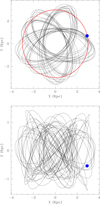 |
Fig. 18. Orbit of M 28 in Galactic cartesian coordinates, in the XY (upper panel) and XZ (lower panel) plane. The blue dot gives the actual position of the cluster, and the red circle indicates the distance of 3 kpc from the Galactic centre. |
Derived cluster parameters.
6. Conclusions
We have analysed wide-field VVV photometric data, VVV proper motions, and intermediate-resolution CaT spectroscopy to study the properties of the bulge globular cluster M 28. The main cluster parameters obtained in this work are presented in Table 3. Our results in general agree with previous measurements in the literature, confirming the properties of this cluster in terms of reddening, distance, and angular size. We also find that the recent estimates of the cluster RV are converging to a value in the range  km s−1, slightly lower than the 17 km s−1 quoted in the Harris (1996, December 2010 web version) catalogue. The orbit, calculated from our measurements of RV, PM, and distance, is confined within 3.8 kpc of the Galactic centre, and 1.4 kpc of the plane. M 28 is therefore a genuine bulge cluster.
The internal RV dispersion of M 28 is high, with a central value of σRV, c = 8.4 ± 0.5 km s−1, from which we obtained a rough estimate of the total cluster mass of  . This should still be an underestimate, both because σRV, c was estimated from stars up to
  from the centre, andbecause of a probable underestimate introduced by the use of a single-mass King model, as discussed in Sect. 5.1. This result places M 28 among the 30% most massive GCs in the Milky Way.
M 28 is undergoing mass loss as a consequence of Galactic tidal forces and shock effects. We detected a tail of stars trailing the cluster in its motion, and a structure directed toward the Galactic plane, as expected by models of GC tidal tails formations (e.g., Küpper et al. 2010; Montuori et al. 2007). In particular, the structures directed toward the Galactic plane and centre are a consequence of relevant tidal shocks from the disk and bulge. Then, despite its present-day high mass, M 28 must have been an even larger structure in the past.
We find that this cluster, with an age of 13–14 Gyr, is one of the oldest objects in the Galactic bulge. We put this result in the context of the bulge evolution history, comparing the age and the metallicity of all bulge GCs with reliable measurements in the literature. The resulting AMR demonstrates that the bulge system evolved quickly, forming clusters 5–10 times more metal-rich than in the halo at the earliest stages, then increasing its metal content by one order of magnitude in about two Gyrs.
Our CaT measurements show no hint of any metallicity inhomogeneity inside the cluster. We found no statistical significance of a double distribution of iron content, and we derived an upper limit to any internal metallicity spread of 0.08 dex. We thus strengthen with a larger statistical sample (32 stars) the result found by V17 in their high-resolution analysis of 17 red giant stars. Hence, M 28 can be considered a classical GC, with large star-to-star variations of light elements (V17), but a homogeneous metallicity.
In conclusion, the age and metallicity of M 28, its orbit, and the absence of chemical peculiarities (V17), support the Bica et al. (2016) classification of a genuine bulge GC. However, its very old age, its high mass, and its evident mass loss suggest that this cluster should be the remnant of a larger structure, possibly a very massive GC or a primeval bulge building block, as previously suggested by Lee et al. (2007) and Chun et al. (2012).
IRAF is distributed by the National Optical Astronomy Observatories, which are operated by the Association of Universities for Research in Astronomy, Inc., under cooperative agreement with the National Science Foundation.
For a more readable notation, in this section and hereafter we use the units mÅ, where 1 mÅ = 10−3 Å.
Acknowledgments
The authors thanks the referee for their very helpful comments and suggestions. C. M. B., S. V., and D. M. acknowledge support from FONDECYT through regular projects 1150060, 1170518, and 1170121. D. M. and D. G. gratefully acknowledge support from the BASAL Centre for Astrophysics and Associated Technologies (CATA) through grant AFB 170002. D. G. also acknowledges financial support from the Dirección de Investigación y Desarrollo de la Universidad de La Serena through the Programa de Incentivo a la Investigación de Académicos (PIA-DIDULS). Support to J. B. and M. Z. is provided by the Ministry for the Economy, Development and Tourism, Programa Iniciativa Científica Milenio grant IC120009, awarded to the Millennium Institute of Astrophysics (MAS), and by ANID, Millennium Science Initiative ICN12_009 awarded to the Millennium Institute of Astrophysics (MAS). A.-N. C. is supported by the Gemini Observatory, which is operated by the Association of Universities for Research in Astronomy, Inc., on behalf of the international Gemini partnership of Argentina, Brazil, Canada, Chile, and the United States of America. We gratefully acknowledge data from the ESO Public Survey program ID 179.B-2002 taken with the VISTA telescope, and products from the Cambridge Astronomical Survey Unit (CASU). This work has made use of data from the European Space Agency (ESA) mission Gaia (https://www.cosmos.esa.int/gaia), processed by the Gaia Data Processing and Analysis Consortium (DPAC, https://www.cosmos.esa.int/web/gaia/dpac/consortium). Funding for the DPAC has been provided by national institutions, in particular the institutions participating in the Gaia Multilateral Agreement. This investigation made use of data from the Two Micron All Sky Survey, which is a joint project of the University of Massachusetts and the Infrared Processing and Analysis Center/California Institute of Technology, funded by the National Aeronautics and Space Administration and the National Science Foundation.
References
- Alonso, A., Arribas, S., & Martinez-Roger, C. 1998, A&AS, 131, 209 [NASA ADS] [CrossRef] [EDP Sciences] [Google Scholar]
- Alonso, A., Arribas, S., & Martínez-Roger, C. 1999, A&AS, 140, 261 [NASA ADS] [CrossRef] [EDP Sciences] [Google Scholar]
- Armandroff, T. E., & Da Costa, G. S. 1991, AJ, 101, 1329 [NASA ADS] [CrossRef] [Google Scholar]
- Armandroff, T. E., & Zinn, R. 1988, AJ, 96, 92 [NASA ADS] [CrossRef] [Google Scholar]
- Ashman, K. M., Bird, C. M., & Zepf, S. E. 1994, AJ, 108, 2348 [NASA ADS] [CrossRef] [Google Scholar]
- Barbuy, B., Zoccali, M., Ortolani, S., et al. 2007, AJ, 134, 1613 [NASA ADS] [CrossRef] [Google Scholar]
- Barbuy, B., Zoccali, M., Ortolani, S., et al. 2009, A&A, 507, 405 [NASA ADS] [CrossRef] [EDP Sciences] [Google Scholar]
- Barbuy, B., Cantelli, E., Vemado, A., et al. 2016, A&A, 591, A53 [NASA ADS] [CrossRef] [EDP Sciences] [Google Scholar]
- Baumgardt, H., & Hilker, M. 2018, MNRAS, 478, 1520 [Google Scholar]
- Baumgardt, H., Hilker, M., Sollima, A., & Bellini, A. 2019, MNRAS, 482, 5138 [Google Scholar]
- Bianchini, P., Norris, M. A., van de Ven, G., et al. 2016, ApJ, 820, L22 [Google Scholar]
- Bica, E., Ortolani, S., & Barbuy, B. 2016, PASA, 33, e028 [NASA ADS] [CrossRef] [Google Scholar]
- Bird, C. M. 1994, AJ, 107, 1637 [NASA ADS] [CrossRef] [Google Scholar]
- Bonifacio, P., Monai, S., & Beers, T. C. 2000, AJ, 120, 2065 [NASA ADS] [CrossRef] [Google Scholar]
- Calamida, A., Bono, G., Lagioia, E. P., et al. 2014, A&A, 565, A8 [NASA ADS] [CrossRef] [EDP Sciences] [Google Scholar]
- Cardelli, J. A., Clayton, G. C., & Mathis, J. S. 1989, ApJ, 345, 245 [NASA ADS] [CrossRef] [Google Scholar]
- Carretta, E., Bragaglia, A., Gratton, R., D’Orazi, V., & Lucatello, S. 2009, A&A, 508, 695 [NASA ADS] [CrossRef] [EDP Sciences] [Google Scholar]
- Carretta, E., Bragaglia, A., Gratton, R. G., et al. 2010, ApJ, 714, L7 [NASA ADS] [CrossRef] [Google Scholar]
- Casetti-Dinescu, D. I., Girard, T. M., Jílková, L., et al. 2013, AJ, 146, 33 [NASA ADS] [CrossRef] [Google Scholar]
- Chemel, A. A., Glushkova, E. V., Dambis, A. K., et al. 2018, Astrophys. Bull., 73, 162 [CrossRef] [Google Scholar]
- Chené, A.-N., Borissova, J., Clarke, J. R. A., et al. 2012, A&A, 545, A54 [NASA ADS] [CrossRef] [EDP Sciences] [Google Scholar]
- Chun, S.-H., Kim, J.-W., Kim, M. J., et al. 2012, AJ, 144, 26 [Google Scholar]
- Chun, S.-H., Kang, M., Jung, D., & Sohn, Y.-J. 2015, AJ, 149, 29 [NASA ADS] [CrossRef] [Google Scholar]
- Coelho, P., Barbuy, B., Meléndez, J., Schiavon, R. P., & Castilho, B. V. 2005, A&A, 443, 735 [NASA ADS] [CrossRef] [EDP Sciences] [Google Scholar]
- Cohen, R. E., Moni Bidin, C., Mauro, F., Bonatto, C., & Geisler, D. 2017, MNRAS, 464, 1874 [Google Scholar]
- Collins, M. L. M., Tollerud, E. J., Sand, D. J., et al. 2017, MNRAS, 467, 573 [Google Scholar]
- Contreras Ramos, R., Zoccali, M., Rojas, F., et al. 2017, A&A, 608, A140 [NASA ADS] [CrossRef] [EDP Sciences] [Google Scholar]
- Cudworth, K. M., & Hanson, R. B. 1993, AJ, 105, 168 [NASA ADS] [CrossRef] [Google Scholar]
- Da Costa, G. S., & Armandroff, T. E. 1995, AJ, 109, 2533 [NASA ADS] [CrossRef] [Google Scholar]
- Da Costa, G. S., Held, E. V., Saviane, I., & Gullieuszik, M. 2009, ApJ, 705, 1481 [NASA ADS] [CrossRef] [Google Scholar]
- D’Antona, F., Caloi, V., Montalbán, J., Ventura, P., & Gratton, R. 2002, A&A, 395, 69 [NASA ADS] [CrossRef] [EDP Sciences] [Google Scholar]
- D’Antona, F., Ventura, P., Caloi, V., et al. 2010, ApJ, 715, L63 [NASA ADS] [CrossRef] [Google Scholar]
- Davidge, T. J., Cote, P., & Harris, W. E. 1996, ApJ, 468, 641 [NASA ADS] [CrossRef] [Google Scholar]
- Decressin, T., Meynet, G., Charbonnel, C., Prantzos, N., & Ekström, S. 2007, A&A, 464, 1029 [NASA ADS] [CrossRef] [EDP Sciences] [Google Scholar]
- de Mink, S. E., Pols, O. R., Langer, N., & Izzard, R. G. 2010, in Star Clusters: Basic Galactic Building Blocks Throughout Time and Space, eds. R. de Grijs, & J. R. D. Lépine, IAU Symp., 266, 169 [Google Scholar]
- de Vaucouleurs, G. 1959, Handbuch der Physik, 53, 275 [Google Scholar]
- Dinescu, D. I., Girard, T. M., & van Altena, W. F. 1999, AJ, 117, 1792 [NASA ADS] [CrossRef] [Google Scholar]
- Dotter, A., Chaboyer, B., Jevremović, D., et al. 2008, ApJS, 178, 89 [Google Scholar]
- Dotter, A., Sarajedini, A., Anderson, J., et al. 2010, ApJ, 708, 698 [NASA ADS] [CrossRef] [Google Scholar]
- Emerson, J., & Sutherland, W. 2010, Messenger, 139, 2 [Google Scholar]
- Feltzing, S., & Johnson, R. A. 2002, A&A, 385, 67 [NASA ADS] [CrossRef] [EDP Sciences] [Google Scholar]
- Fernandez-Trincado, J. G. 2017, PhD Thesis, University Bourgogne-Franche-Comté, France [Google Scholar]
- Ferraro, F. R., Dalessandro, E., Mucciarelli, A., et al. 2009, Nature, 462, 483 [NASA ADS] [CrossRef] [PubMed] [Google Scholar]
- Gaia Collaboration (Prusti, T., et al.) 2016, A&A, 595, A1 [NASA ADS] [CrossRef] [EDP Sciences] [Google Scholar]
- Gaia Collaboration (Helmi, A., et al.) 2018a, A&A, 616, A12 [NASA ADS] [CrossRef] [EDP Sciences] [Google Scholar]
- Gaia Collaboration (Brown, A. G. A., et al.) 2018b, A&A, 616, A1 [NASA ADS] [CrossRef] [EDP Sciences] [Google Scholar]
- Gallart, C., Zoccali, M., Bertelli, G., et al. 2003, AJ, 125, 742 [NASA ADS] [CrossRef] [Google Scholar]
- Goldsbury, R., Richer, H. B., Anderson, J., et al. 2010, AJ, 140, 1830 [NASA ADS] [CrossRef] [Google Scholar]
- Hamaker, H. C. 1978, Appl. Stat., 27, 76 [Google Scholar]
- Harris, W. E. 1996, AJ, 112, 1487 [NASA ADS] [CrossRef] [Google Scholar]
- Hempel, M., Minniti, D., Dékány, I., et al. 2014, Messenger, 155, 24 [Google Scholar]
- Hesser, J. E., Shawl, S. J., & Meyer, J. E. 1986, PASP, 98, 403 [NASA ADS] [CrossRef] [Google Scholar]
- Horne, K. 1986, PASP, 98, 609 [NASA ADS] [CrossRef] [EDP Sciences] [Google Scholar]
- Illingworth, G. 1976, ApJ, 204, 73 [NASA ADS] [CrossRef] [Google Scholar]
- Illingworth, G., & Illingworth, W. 1976, ApJS, 30, 227 [Google Scholar]
- Irwin, M. J., Lewis, J., Hodgkin, S., et al. 2004, in Society of Photo-Optical Instrumentation Engineers (SPIE) Conference Series, eds. P. J. Quinn, A. Bridger, et al., 5493, 411 [Google Scholar]
- Johnson, C. I., Pilachowski, C. A., Simmerer, J., & Schwenk, D. 2008, ApJ, 681, 1505 [NASA ADS] [CrossRef] [Google Scholar]
- Johnson, C. I., Rich, R. M., Caldwell, N., et al. 2018, AJ, 155, 71 [CrossRef] [Google Scholar]
- Kerber, L. O., Nardiello, D., Ortolani, S., et al. 2018, ApJ, 853, 15 [NASA ADS] [CrossRef] [Google Scholar]
- Kerber, L. O., Libralato, M., Souza, S. O., et al. 2019, MNRAS, 484, 5530 [NASA ADS] [CrossRef] [Google Scholar]
- King, I. 1962, AJ, 67, 471 [NASA ADS] [CrossRef] [Google Scholar]
- King, I. R. 1966, AJ, 71, 64 [Google Scholar]
- Kinman, T. D. 1959, MNRAS, 119, 157 [NASA ADS] [Google Scholar]
- Kundu, R., Minniti, D., & Singh, H. P. 2019, MNRAS, 483, 1737 [NASA ADS] [CrossRef] [Google Scholar]
- Küpper, A. H. W., Kroupa, P., Baumgardt, H., & Heggie, D. C. 2010, MNRAS, 401, 105 [NASA ADS] [CrossRef] [Google Scholar]
- Lagioia, E. P., Milone, A. P., Stetson, P. B., et al. 2014, ApJ, 782, 50 [NASA ADS] [CrossRef] [Google Scholar]
- Lanzoni, B., Ferraro, F. R., Dalessandro, E., et al. 2010, ApJ, 717, 653 [NASA ADS] [CrossRef] [Google Scholar]
- Leaman, R., VandenBerg, D. A., & Mendel, J. T. 2013, MNRAS, 436, 122 [NASA ADS] [CrossRef] [Google Scholar]
- Lee, J.-W. 2016, ApJS, 226, 16 [NASA ADS] [CrossRef] [Google Scholar]
- Lee, M. G., & Geisler, D. 1993, AJ, 106, 493 [NASA ADS] [CrossRef] [Google Scholar]
- Lee, Y.-W., Gim, H. B., & Casetti-Dinescu, D. I. 2007, ApJ, 661, L49 [NASA ADS] [CrossRef] [Google Scholar]
- Lee, J.-W., Kang, Y.-W., Lee, J., & Lee, Y.-W. 2009, Nature, 462, 480 [NASA ADS] [CrossRef] [PubMed] [Google Scholar]
- Lucatello, S., Sollima, A., Gratton, R., et al. 2015, A&A, 584, A52 [NASA ADS] [CrossRef] [EDP Sciences] [Google Scholar]
- Lutz, T. E., & Hanson, R. B. 1992, in Astronomical Data Analysis Software and Systems I, eds. D. M. Worrall, C. Biemesderfer, & J. Barnes, ASP Conf. Ser., 25, 257 [Google Scholar]
- Mandushev, G., Staneva, A., & Spasova, N. 1991, A&A, 252, 94 [NASA ADS] [Google Scholar]
- Marino, A. F., Milone, A. P., Piotto, G., et al. 2009, A&A, 505, 1099 [NASA ADS] [CrossRef] [EDP Sciences] [Google Scholar]
- Marino, A. F., Sneden, C., Kraft, R. P., et al. 2011, A&A, 532, A8 [NASA ADS] [CrossRef] [EDP Sciences] [Google Scholar]
- Mashonkina, L. I., Sitnova, T. N., & Pakhomov, Y. V. 2016, Astron. Lett., 42, 606 [NASA ADS] [CrossRef] [Google Scholar]
- Mauro, F., Moni Bidin, C., Cohen, R., et al. 2012, ApJ, 761, L29 [NASA ADS] [CrossRef] [Google Scholar]
- Mauro, F., Moni Bidin, C., Chené, A.-N., et al. 2013, RM&AC, 49, 189 [Google Scholar]
- Mauro, F., Moni Bidin, C., Geisler, D., et al. 2014, A&A, 563, A76 [NASA ADS] [CrossRef] [EDP Sciences] [Google Scholar]
- Mayall, N. U. 1946, ApJ, 104, 290 [NASA ADS] [CrossRef] [Google Scholar]
- McLachlan, G. J., & Basford, K. E. 1988, Mixture Models. Inference and Applications to Clustering (New York: Dekker) [Google Scholar]
- Meissner, F., & Weiss, A. 2006, A&A, 456, 1085 [NASA ADS] [CrossRef] [EDP Sciences] [Google Scholar]
- Minniti, D. 1995a, A&AS, 113, 299 [NASA ADS] [Google Scholar]
- Minniti, D. 1995b, AJ, 109, 1663 [NASA ADS] [CrossRef] [Google Scholar]
- Minniti, D., Lucas, P. W., Emerson, J. P., et al. 2010, New A, 15, 433 [NASA ADS] [CrossRef] [Google Scholar]
- Miocchi, P., Lanzoni, B., Ferraro, F. R., et al. 2013, ApJ, 774, 151 [NASA ADS] [CrossRef] [Google Scholar]
- Momany, Y., Ortolani, S., Held, E. V., et al. 2003, A&A, 402, 607 [NASA ADS] [CrossRef] [EDP Sciences] [Google Scholar]
- Moni Bidin, C., Mauro, F., Geisler, D., et al. 2011, A&A, 535, A33 [NASA ADS] [CrossRef] [EDP Sciences] [Google Scholar]
- Moni Bidin, C., Carraro, G., & Méndez, R. A. 2012, ApJ, 747, 101 [NASA ADS] [CrossRef] [Google Scholar]
- Montuori, M., Capuzzo-Dolcetta, R., Di Matteo, P., Lepinette, A., & Miocchi, P. 2007, ApJ, 659, 1212 [NASA ADS] [CrossRef] [Google Scholar]
- Mottini, M., & Wallerstein, G. 2008, AJ, 136, 731 [NASA ADS] [CrossRef] [Google Scholar]
- Mucciarelli, A., Lapenna, E., Massari, D., et al. 2015, ApJ, 809, 128 [Google Scholar]
- Muñoz, C., Villanova, S., Geisler, D., et al. 2017, A&A, 605, A12 [NASA ADS] [CrossRef] [EDP Sciences] [Google Scholar]
- Muñoz, C., Geisler, D., Villanova, S., et al. 2018, A&A, 620, A96 [NASA ADS] [CrossRef] [EDP Sciences] [Google Scholar]
- Myeong, G. C., Vasiliev, E., Iorio, G., Evans, N. W., & Belokurov, V. 2019, MNRAS, 488, 1235 [Google Scholar]
- Noyola, E., & Gebhardt, K. 2006, AJ, 132, 447 [NASA ADS] [CrossRef] [Google Scholar]
- Olszewski, E. W., Schommer, R. A., Suntzeff, N. B., & Harris, H. C. 1991, AJ, 101, 515 [Google Scholar]
- Origlia, L., Rich, R. M., Ferraro, F. R., et al. 2011, ApJ, 726, L20 [Google Scholar]
- Ostrov, P., Geisler, D., & Forte, J. C. 1993, AJ, 105, 1762 [NASA ADS] [CrossRef] [Google Scholar]
- Pasquini, L., Avila, G., Blecha, A., et al. 2002, Messenger, 110, 1 [NASA ADS] [Google Scholar]
- Peterson, C. J., & Reed, B. C. 1987, PASP, 99, 20 [NASA ADS] [CrossRef] [Google Scholar]
- Pietrinferni, A., Cassisi, S., Salaris, M., & Castelli, F. 2006, ApJ, 642, 797 [NASA ADS] [CrossRef] [Google Scholar]
- Piotto, G., Villanova, S., Bedin, L. R., et al. 2005, ApJ, 621, 777 [NASA ADS] [CrossRef] [Google Scholar]
- Piotto, G., Milone, A. P., Bedin, L. R., et al. 2015, AJ, 149, 91 [NASA ADS] [CrossRef] [Google Scholar]
- Poleski, R. 2013, ArXiv e-prints [arXiv:1306.2945] [Google Scholar]
- Prieto, G., Catelan, M., Contreras Ramos, R., et al. 2012, A&A, 543, A148 [EDP Sciences] [Google Scholar]
- Pryor, C., & Meylan, G. 1993, in Structure and Dynamics of Globular Clusters, eds. S. G. Djorgovski, & G. Meylan, ASP Conf. Ser., 50, 357 [Google Scholar]
- Pryor, C., McClure, R. D., Fletcher, J. M., & Hesser, J. E. 1989, AJ, 98, 596 [Google Scholar]
- Reed, B. C., Hesser, J. E., & Shawl, S. J. 1988, PASP, 100, 545 [NASA ADS] [CrossRef] [Google Scholar]
- Renzini, A., D’Antona, F., Cassisi, S., et al. 2015, MNRAS, 454, 4197 [NASA ADS] [CrossRef] [Google Scholar]
- Robin, A. C., Reylé, C., Derrière, S., & Picaud, S. 2003, A&A, 409, 523 [NASA ADS] [CrossRef] [EDP Sciences] [Google Scholar]
- Robin, A. C., Marshall, D. J., Schultheis, M., & Reylé, C. 2012, A&A, 538, A106 [NASA ADS] [CrossRef] [EDP Sciences] [Google Scholar]
- Roediger, J. C., Courteau, S., Graves, G., & Schiavon, R. P. 2014, ApJS, 210, 10 [Google Scholar]
- Rutledge, G. A., Hesser, J. E., Stetson, P. B., et al. 1997, PASP, 109, 883 [Google Scholar]
- Saito, R. K., Hempel, M., Minniti, D., et al. 2012, A&A, 537, A107 [NASA ADS] [CrossRef] [EDP Sciences] [Google Scholar]
- Salgado, C., Moni Bidin, C., Villanova, S., Geisler, D., & Catelan, M. 2013, A&A, 559, A101 [NASA ADS] [CrossRef] [EDP Sciences] [Google Scholar]
- Saracino, S., Dalessandro, E., Ferraro, F. R., et al. 2016, ApJ, 832, 48 [NASA ADS] [CrossRef] [Google Scholar]
- Saracino, S., Dalessandro, E., Ferraro, F. R., et al. 2019, ApJ, 874, 86 [Google Scholar]
- Saviane, I., da Costa, G. S., Held, E. V., et al. 2012, A&A, 540, A27 [NASA ADS] [CrossRef] [EDP Sciences] [Google Scholar]
- Sbordone, L., Monaco, L., Moni Bidin, C., et al. 2015, A&A, 579, A104 [NASA ADS] [CrossRef] [EDP Sciences] [Google Scholar]
- Schlafly, E. F., & Finkbeiner, D. P. 2011, ApJ, 737, 103 [NASA ADS] [CrossRef] [Google Scholar]
- Schlegel, D. J., Finkbeiner, D. P., & Davis, M. 1998, ApJ, 500, 525 [NASA ADS] [CrossRef] [Google Scholar]
- Schönrich, R., Binney, J., & Dehnen, W. 2010, MNRAS, 403, 1829 [NASA ADS] [CrossRef] [Google Scholar]
- Shapiro, S. S., & Wilk, M. B. 1965, Biometrika, 52, 591 [Google Scholar]
- Simkin, S. M. 1974, A&A, 31, 129 [NASA ADS] [Google Scholar]
- Sitnova, T., Zhao, G., Mashonkina, L., et al. 2015, ApJ, 808, 148 [Google Scholar]
- Skrutskie, M. F., Cutri, R. M., Stiening, R., et al. 2006, AJ, 131, 1163 [NASA ADS] [CrossRef] [Google Scholar]
- Stetson, P. B. 1994, PASP, 106, 250 [NASA ADS] [CrossRef] [Google Scholar]
- Testa, V., Corsi, C. E., Andreuzzi, G., et al. 2001, AJ, 121, 916 [NASA ADS] [CrossRef] [Google Scholar]
- Tonry, J., & Davis, M. 1979, AJ, 84, 1511 [NASA ADS] [CrossRef] [Google Scholar]
- Trager, S. C., Djorgovski, S., & King, I. R. 1993, in Structure and Dynamics of Globular Clusters, eds. S. G. Djorgovski, & G. Meylan, ASP Conf. Ser., 50, 347 [Google Scholar]
- van den Bergh, S., Morbey, C., & Pazder, J. 1991, ApJ, 375, 594 [NASA ADS] [CrossRef] [Google Scholar]
- VandenBerg, D. A., Brogaard, K., Leaman, R., & Casagrande, L. 2013, ApJ, 775, 134 [NASA ADS] [CrossRef] [Google Scholar]
- Vasiliev, E. 2019, MNRAS, 484, 2832 [NASA ADS] [CrossRef] [Google Scholar]
- Villanova, S., Geisler, D., Carraro, G., Moni Bidin, C., & Muñoz, C. 2013, ApJ, 778, 186 [NASA ADS] [CrossRef] [Google Scholar]
- Villanova, S., Moni Bidin, C., Mauro, F., Munoz, C., & Monaco, L. 2017, MNRAS, 464, 2730 [NASA ADS] [CrossRef] [Google Scholar]
- Watkins, L. L., van der Marel, R. P., Bellini, A., & Anderson, J. 2015, ApJ, 803, 29 [Google Scholar]
- Webbink, R. F. 1981, ApJS, 45, 259 [NASA ADS] [CrossRef] [Google Scholar]
- Webbink, R. F. 1985, in Dynamics of Star Clusters, eds. J. Goodman, & P. Hut, IAU Symp., 113, 541 [Google Scholar]
- Zinn, R. 1985, ApJ, 293, 424 [Google Scholar]
- Zoccali, M., Renzini, A., Ortolani, S., Bica, E., & Barbuy, B. 2001, AJ, 121, 2638 [NASA ADS] [CrossRef] [Google Scholar]
Appendix A: Additional table
Data of the observed target stars.
All Tables
All Figures
|
Fig. 1. Photometric errors as a function of magnitude in the J (blue), H (light blue), and Ks (black) bands. |
| In the text | |
|
Fig. 2. Density map of the sources with Ks < 17.5 detected in the VVV frames. The density values in the blue-scale bar are in units of sources per arcmin2. The contour levels are shown at steps of 25 sources arcmin−2 from the minimum average background. |
| In the text | |
|
Fig. 3. Position of the spectroscopic targets in the VVV colour-magnitude diagram. The sources detected within 2′ of the cluster centre are overplotted in light blue. Solid dots, open symbols, and crosses indicate the stars classified as cluster members, additional member candidates, and field stars, respectively. Average errors as a function of magnitudes are plotted on the right, and the arrow shows the direction of interstellar reddening. |
| In the text | |
|
Fig. 4. Radial density profile of detected sources with Ks < 16. The curve shows the best-fit King profile in the range r = 2−13′. |
| In the text | |
|
Fig. 5. Original (blue dots) and decontaminated (black dots) CMD of the cluster area (r < 4′). The arrow and the error bars are as in Fig. 3. The dotted line shows the saturation limit in VVV frames. |
| In the text | |
|
Fig. 6. Hess diagram of the decontaminated cluster CMD (left panel), and of a synthetic CMD calculated from the cluster isochrone and the photometric errors (right panel). |
| In the text | |
|
Fig. 7. Fiducial line of the cluster sequence (squares), and the best-fit DSED isochrones for τ = 12.5, 13.5, and 14.5 Gyr (dotted, full, and dashed curve, respectively). The decontaminated cluster CMD is shown as light blue points. |
| In the text | |
|
Fig. 8. Comparison between the V17 results (filled dots) and DSED isochrones (full curves), in the temperature-gravity plane. The errors shown are the internal uncertainties from V17. |
| In the text | |
|
Fig. 9. VVV relative proper motions of stars in the cluster sequence (black dots), superimposed on the distribution of field stars. |
| In the text | |
|
Fig. 10. Upper panel: normalised background-subtracted density map of the cluster area, in units of the background noise (σ). Contour levels are shown at 3σ, 4σ, and 5σ. The full white arrow shows the direction of the cluster proper motion, while the dashed arrow points toward the Galactic centre. Lower panel: Schlegel et al. (1998) reddening map of the same area as the upper panel. The reddening values in the greyscale bar are given in E(B − V). |
| In the text | |
|
Fig. 11. Histogram of RV distribution of all spectroscopic targets (blue histogram), and targets within 4′ from the cluster centre (black histogram). |
| In the text | |
|
Fig. 12. Radial profile of the RV dispersion deduced from our sample. The big black dots are obtained binning our sample in steps of |
| In the text | |
|
Fig. 13. Relative proper motion of the spectroscopic targets, according to our classification: dwarf stars and non-members (filled and empty blue dots), cluster members and probable cluster members (full and empty black dots). The large and small ellipses are centred on the cluster and field mean value, respectively, with semi-axis equal to the standard deviation of the distributions. |
| In the text | |
|
Fig. 14. Sum of the EW of the three CaT lines (ΣEW) of target stars, as a function of their magnitude difference with respect to the HB level (ΔKs). Full and empty dots are used for the cluster members and the additional possible cluster members, respectively. The line shows the linear fit of the cluster members. |
| In the text | |
|
Fig. 15. Histogram of distribution of ΔΣEW for the observed targets. Different algorithms are shown, as detailed in the text. |
| In the text | |
|
Fig. 16. Absolute luminosity in the V band as a function of the central RV dispersion of all GCs in the Harris (1996) catalogue with available measurements. The black dot represents M 28, with our dispersion measurement. |
| In the text | |
|
Fig. 17. Age-metallicity relation of bulge clusters. The dashed line indicates the linear fit of the data, while the dotted line shows a similar relation for halo objects. Empty light blue dots are used for the single literature measurements, while full black dots show the average value for each cluster. The outlier NGC 6553 is shown as a triangle, while M 28 is shown as a larger diamond. |
| In the text | |
|
Fig. 18. Orbit of M 28 in Galactic cartesian coordinates, in the XY (upper panel) and XZ (lower panel) plane. The blue dot gives the actual position of the cluster, and the red circle indicates the distance of 3 kpc from the Galactic centre. |
| In the text | |
Current usage metrics show cumulative count of Article Views (full-text article views including HTML views, PDF and ePub downloads, according to the available data) and Abstracts Views on Vision4Press platform.
Data correspond to usage on the plateform after 2015. The current usage metrics is available 48-96 hours after online publication and is updated daily on week days.
Initial download of the metrics may take a while.