| Issue |
A&A
Volume 647, March 2021
|
|
|---|---|---|
| Article Number | A194 | |
| Number of page(s) | 13 | |
| Section | Extragalactic astronomy | |
| DOI | https://doi.org/10.1051/0004-6361/202039807 | |
| Published online | 02 April 2021 | |
Fast rotating and low-turbulence discs at z ≃ 4.5: Dynamical evidence of their evolution into local early-type galaxies
1
Kapteyn Astronomical Institute, University of Groningen, Postbus 800, 9700 AV Groningen, The Netherlands
e-mail: This email address is being protected from spambots. You need JavaScript enabled to view it.
2
Argelander Institut für Astronomie, Universität Bonn, Auf dem Hügel 71, Bonn 53121, Germany
3
AIM, CEA, CNRS, Université Paris-Saclay, Université Paris Diderot, Sorbonne Paris Cité, 91191 Gif-sur-Yvette, France
4
National Radio Astronomy Observatory, 520 Edgemont Road, Charlottesville, VA 22903, USA
5
Núcleo de Astronomía, Facultad de Ingeniería y Ciencias, Universidad Diego Portales, Av. Ejército 441, Santiago, Chile
Received:
30
October
2020
Accepted:
2
February
2021
Abstract
Massive starburst galaxies in the early Universe are estimated to have depletion times of ∼100 Myr and thus be able to convert their gas very quickly into stars, possibly leading to a rapid quenching of their star formation. For these reasons, they are considered progenitors of massive early-type galaxies (ETGs). In this paper, we study two high-z starbursts, AzTEC/C159 (z ≃ 4.57) and J1000+0234 (z ≃ 4.54), observed with ALMA in the [C II] 158-μm emission line. These observations reveal two massive and regularly rotating gaseous discs. A 3D modelling of these discs returns rotation velocities of about 500 km s−1 and gas velocity dispersions as low as ≈ 20 km s−1, leading to very high ratios between regular and random motion (V/σ ≳ 20), at least in AzTEC/C159. The mass decompositions of the rotation curves show that both galaxies are highly baryon-dominated with gas masses of ≈1011 M⊙, which, for J1000+0234, is significantly higher than previous estimates. We show that these high-z galaxies overlap with z = 0 massive ETGs in the ETG analogue of the stellar-mass Tully-Fisher relation once their gas is converted into stars. This provides dynamical evidence of the connection between massive high-z starbursts and ETGs, although the transformation mechanism from fast rotating to nearly pressure-supported systems remains unclear.
Key words: galaxies: formation / galaxies: evolution / galaxies: kinematics and dynamics / galaxies: high-redshift / galaxies: starburst
© ESO 2021
1. Introduction
Over the last decade, we have witnessed the accumulation of stunning new data that are changing our view of very distant galaxies down to the early epochs of their formation. The dynamics of high-z galaxies can be very efficiently studied using a variety of emission lines. Optical recombination and forbidden lines are mostly used in the redshift range 0 ≲ z ≲ 3.5 (e.g. Förster Schreiber et al. 2009; Stott et al. 2016; Turner et al. 2017), while at z ≳ 4 the main contribution has come from CO and [C II] 158-μm data (e.g. Carilli & Walter 2013).
One of the most surprising results to have emerged is the ubiquitous presence of rotating gaseous discs in high-z galaxies (e.g. Genzel et al. 2006). Initial estimates of the amount of rotation-dominated galaxies of around 30% (Förster Schreiber et al. 2009) have been significantly revised to the point that the dynamics of the vast majority of galaxies at z ≈ 1 − 5 is now considered to be dominated by rotation (Wisnioski et al. 2019; Lelli et al. 2018, 2021; Loiacono et al. 2019; Neeleman et al. 2020; Rizzo et al. 2020). This revision has been the consequence of major improvements in the quality of the data and data analysis. Kinematic data of high-z galaxies suffer two main shortcomings: low angular resolutions and a low signal-to-noise ratio (S/N). Both, however, have improved in recent years thanks, for instance, to the use of adaptive optics (AO) techniques in the optical (Förster Schreiber et al. 2018) and the progressive addition of new antennas to the Atacama Large Millimeter/submillimeter Array (ALMA) interferometer.
The second advance of recent years has been the development of new software that allows the extraction of the entirety of the information contained in data cubes (e.g. Di Teodoro & Fraternali 2015; Bouché et al. 2015). The kinematics of disc (rotation-dominated) galaxies is studied by modelling the galaxy as a series of concentric rings characterised by different geometrical and kinematic parameters (tilted-ring model; Rogstad et al. 1974). Emission-line velocity fields can be easily fitted with a tilted-ring model to extract the rotation curve when the galaxy is observed at high angular resolution, as what happens for nearby systems (e.g. Battaglia et al. 2006; de Blok et al. 2008). However, as the angular resolution decreases, line profiles from different parts of the disc, characterised by different line-of-sight velocities, blend together in the same resolution element, an effect known as ‘beam smearing’ (Swaters et al. 2009). The best way to correct for this observational bias is to build artificial observations (3D tilted-ring models) and compared them directly with the emission in the data cube, without extracting 2D maps. A public code that carries out this type of analysis is 3DBAROLO (Di Teodoro & Fraternali 2015), which we use in this work.
This paper focuses on two starburst galaxies at z ≈ 4.5 observed with ALMA in the [C II] 158-μm emission line. Starburst high-z galaxies are characterised by intense emission at wavelengths from far-infrared (FIR) to millimetre due to the re-processing of the ultraviolet (UV) light produced by young stars (e.g. Casey et al. 2014). A sub-class of these sources, selected for their particularly strong sub-millimetre emission, are called sub-millimetre galaxies (SMGs; Weiß et al. 2009; Karim et al. 2013). The typical star formation rate (SFR) of these startbursts is of the order of hundreds of M⊙ yr−1 (da Cunha et al. 2015), though exceeding 1000 M⊙ yr−1 in some cases (Magnelli et al. 2012; Swinbank et al. 2014; Jiménez-Andrade et al. 2020). These galaxies also have very high stellar masses, M⋆ ∼ 1011 M⊙, leading to a specific star formation rate (sSFR) of ∼10−8 yr−1, which is characteristic of systems that are building their stellar component extremely rapidly (Gómez-Guijarro et al. 2018; Lang et al. 2019; Dudzevičiūtė et al. 2020). Estimates of the gas mass in massive high-z starbursts return values comparable with their stellar mass; this gas is thought to be mostly in molecular form (Ivison et al. 2010; Harrington et al. 2018). The depletion times (MH2/SFR) are very short (∼100 Myr), again pointing at a rapid transformation of their gas reservoir into stars (Jiménez-Andrade et al. 2020; Birkin et al. 2021).
The environment of high-z starbursts is thought to be violent and highly dynamic. On the one hand, the extreme star formation activity in the galaxy is likely the consequence of a major merger or powerful gas accretion from the surroundings (Riechers et al. 2011; Aguirre et al. 2013; Jiménez-Andrade et al. 2020). On the other, star formation at these extraordinary rates is expected to cause intense supernova feedback that can eject a large portion of the gas (e.g. Hayward & Hopkins 2017). Active galactic nuclei (AGNs) are also observed in high-z starbursts, providing additional energy injection into the surrounding gas (e.g. Zeballos et al. 2018).
The kinematics of galaxies at z ≳ 4 has, until recent years, been challenging to study. Rest-frame optical emission lines cannot be used at these high redshifts, while the Lyα line, due to resonant scattering, does not constitute a reliable kinematic tracer (e.g. Cantalupo et al. 2019). Before the advent of ALMA, pioneering works provided indications of high rotation velocities using CO emission lines (Greve et al. 2005). Observations with the Very Large Array (VLA) have given the first clear resolved observation of a regularly rotating disc in the SMG GN20 (Hodge et al. 2012). These authors reported a CO disc extending to a radius of about 7 kpc and with a rotation exceeding 500 km s−1, assuming an inclination of the disc of 30°. The dynamics of high-z galaxies and AGNs has also been studied with the [C II] 158-μm line, which is the brightest atomic fine-structure line in the interstellar medium (ISM) and is thought to be a good tracer of both molecular and atomic gas (Carilli & Walter 2013). This field has been revolutionised by ALMA, which led to the detection of several systems displaying regular gas kinematics (Carniani et al. 2013; De Breuck et al. 2014; Oteo et al. 2016; Jones et al. 2017). These galaxies tend to show very high rotation velocities, a signature of a population of massive objects, but less massive discs are also coming into reach (Neeleman et al. 2020; Rizzo et al. 2020).
Massive high-z starbursts, and SMGs in particular, are thought to be progenitors of present-day (passive) early-type galaxies (ETGs; Cimatti et al. 2008; Fu et al. 2013; Toft et al. 2014; Gómez-Guijarro et al. 2018). Indeed, due to their extremely high SFRs, they form most of their stellar component at z > 2 and are expected to have a sharp decline in their star formation history thereafter. This hypothesis can also be tested dynamically, by investigating the shape of their gravitation potential. Here we present a dynamical study of two starburst galaxies at z ≈ 4.5, AzTEC/C159 and J1000+0234, observed with ALMA in the [C II] 158-μm transition. Our 3D approach reveals the existence of fast rotating and remarkably low-turbulence discs in these galaxies. Section 2 presents the physical properties of our two galaxies. Section 3 describes the 3D kinematic modelling of both galaxies and our main results, while Sect. 4 discusses the reliability of our measures and the possible future evolution of our starbursts. Section 5 sums up. Throughout the paper we use Planck cosmological parameters (Planck Collaboration VI 2020).
2. Galaxy and data presentation
We present results for two galaxies at z ≈ 4.5, AzTEC/C159 and J1000+0234, observed with ALMA in the [C II] 158-μm fine-structure transition. AzTEC/C159 was first detected through the ASTE/AzTEC-COSMOS 1.1- mm survey (Aretxaga et al. 2011). It is located at z ≃ 4.57 and has an estimated SFR ≈ 700 M⊙ yr−1 and a stellar mass M⋆ ≃ 4.5 ± 0.4 × 10¹⁰ M⊙ (Smolčić et al. 2015; Gómez-Guijarro et al. 2018). Low angular resolution observations in CO (J = 2 → 1) and CO (J = 5 → 4) revealed a tentative double-peaked profile consistent with a rotating disc (Jiménez-Andrade et al. 2018). The total mass of molecular gas is MH2 ≃ 1.5 ± 0.3 × 10¹¹ M⊙, estimated using an αCO factor of 4.3 M⊙(K km s−1 pc 2)−1 (see details in Jiménez-Andrade et al. 2018). Gómez-Guijarro et al. (2018) also estimated an effective radius of  at rest-frame FIR wavelengths, which is indicative of a very compact object. The galaxy is not detected by the Hubble Space Telescope (HST) in the F814W filter and was unfortunately not observed in the infrared (IR) filters (Gómez-Guijarro et al. 2018). We report the main physical properties of AzTEC/C159 in Table 1.
Physical properties of AzTEC/C159.
J1000+0234 (also known as AzTEC/C17) was selected as a V-band dropout in the COSMOS field and appears as a 3-σ detection in JCMT/AzTEC-COSMOS. It is located at z ≃ 4.54 and has an IR-estimated SFR of 440 M⊙ yr−1 with large uncertainties (Table 2). Its stellar mass is also rather uncertain: Smolčić et al. (2015) reported a value of 8.7 × 10¹⁰ M⊙, while Gómez-Guijarro et al. (2018) obtained 1.4 × 10¹⁰ M⊙. Both authors fit the spectral energy distribution (SED) of J1000+0234 but used different techniques and considered different sizes for the actual source (see Gómez-Guijarro et al. 2018, for details). J1000+0234 appears in HST images as being composed of two sources with confirmed similar redshifts (Capak et al. 2008). These are visible in the top left panel of Fig. 4: The first is clearly associated with the [C II] emission, while the second is located in the south and is significantly outside the region of the line emission. The source on the west side of the HST image is a foreground galaxy. Because of this peculiar configuration and the large velocity offset revealed by the Lyα emission (Capak et al. 2008), J1000+0234 has been classified as a merger. Table 2 summarises the physical properties of this galaxy.
Physical properties of J1000+0234.
With 870- μm flux densities of ≈7 mJy, as measured from the continuum emission observed in the line-free band-7 channels, both AzTEC/C159 and J1000+0234 form part of the unblended bright field population of sub-millimetre sources (e.g. Karim et al. 2013; Stach et al. 2018; Simpson et al. 2020). Given that the bulk of these SMGs that have been interferometrically detected at 870- μm flux densities above 6 mJy reside at much lower redshifts (zmed = 2.9, Simpson et al. 2020) compared to our two galaxies, they belong to a rather rare sub-class of the broader SMG population. In the following, we refer to these two galaxies as starbursts (see also Gómez-Guijarro et al. 2018) given that the available constraints for their stellar mass content and ongoing star formation activity places them above the z ≳ 4 main sequence of star forming galaxies (Steinhardt et al. 2014; Caputi et al. 2017; Iyer et al. 2018). However, it should be noted that more robust constraints, in particular of their stellar mass budget and spatial distribution (e.g. through observations with the James Webb Space Telescope), are needed to clarify their starburst nature.
Our two starburst galaxies were observed during ALMA Cycle 2 (program 2012.1.00978.S; PI: A. Karim) in June 2014. They were part of an original sample of the only seven spectroscopically confirmed (Ly-α detection using Keck/DEIMOS) z ≳ 4 galaxies in the COSMOS field (e.g. Schinnerer et al. 2008). The ALMA band 7 was used to cover the emission of [C II] 158-μm at z ≈ 4.5. Only three galaxies of the original sample were eventually observed, the third being Vd-17871, which we do not present here as the data are not of sufficient quality for a reliable kinematic fit. Standard data reduction was carried out using CASA; details can be found in Gómez-Guijarro et al. (2018). Data cubes were produced using a standard Briggs robust parameter of 0.5 and 2, leading to slightly different angular resolutions (less than a 10% difference). For the present analysis, we used data cubes with robust=2 (which maximises the S/N) for AzTEC/C159 and robust=0.5 (a compromise between resolution and S/N) for J1000+0234. For both sources, we produced data cubes with different channel separations. The low spectral resolution data cube, with a channel separation of ≈ 25 km s−1, has a higher S/N per channel and gives the most reliable kinematic fit and a better comparison between data and models. The high spectral resolution data, with a channel separation of ≈ 10 km s−1, were used to better constrain the (intrinsic) gas velocity dispersion in AzTEC/C159 (Sect. 3.5). We note that in this type of data, the channel separation can be considered equal to the velocity resolution (full width at half maximum) of the data. The observational properties of the data cubes are given in Tables 3 and 4.
[C II] observational properties of AzTEC/C159.
[C II] observational properties of J1000+0234.
3. Data analysis and results
We analysed our data with the software 3DBAROLO (Di Teodoro & Fraternali 2015) in order to characterise the source geometry and the kinematics of the gas. In this section, we present the rotation curves and velocity dispersions obtained for both galaxies, first using the low spectral resolution (but high S/N) data cubes and then focusing on the velocity dispersion of AzTEC/C159 at high spectral resolution. Throughout this paper, we use the term ‘velocity dispersion’ to refer to the intrinsic value, corrected for instrumental effects (spatial and spectral resolution). The non-corrected quantity is referred to as the ‘broadening’ of the emission line.
3.1. 3D kinematic fit of AzTEC/C159
The total-flux map and velocity field of the [C II] 158-μm emission of AzTEC/C159 obtained with the low spectral resolution data cube (Table 3) are shown in the top panels of Fig. 1. The total-flux map (analogous to a zeroth moment) has been constructed by summing the emission across all channel maps after the application of a mask. The mask is calculated by 3DBAROLO through smoothing and clipping the data cube, followed by a source detection in the 3D space (Di Teodoro & Fraternali 2015). After several experiments with either only smoothing and clipping or only source detection, we found that a combination of the two produces the best result of a mask that is not too tight around the emission but also not so large as to include too much noise. The top left panel of Fig. 1 shows the total-flux map in contours1 overlaid on an HST image at the location of AzTEC/C159; it shows no detection in the F814W filter, which roughly corresponds to rest-frame far-UV. This lack of detection is likely due to the intense dust absorption (Gómez-Guijarro et al. 2018). The detection in IR with Spitzer Infrared Array Camera (IRAC) is compact and does not give us information about the morphology of this source (see Fig. 1 in Smolčić et al. 2015).
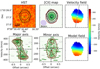 |
Fig. 1. [C II] 158-μm observations and modelling of AzTEC/C159. Top left panel: HST F814W image with the [C II] 158-μm total-flux map contours overlaid; the source is not detected by HST. Top middle panel: total-flux map (green shape and black contours) of the [C II] 158-μm emission; the lowest contour is at about 2.5 times the rms noise in this map, and the other contours are at 2, 4, and 8 times this level. In red we show the outer contour of the total-flux map of the model obtained with 3DBAROLO (convoluted with the observational beam, shown in the bottom left corner). Top right panel: velocity (weighted-mean) field of the [C II] 158-μm line. Bottom left panel: position-velocity diagram along the kinematic major axis of the galaxy (grey line across the velocity field); the data are in green shades and contours, while the best-fit 3DBAROLO model is in red contours. Contour levels are at −2, 2, 4, and 8 times the rms noise per channel. Bottom centre panel: position-velocity diagram along the kinematic minor axis of the galaxy displayed analogously to the major-axis plot. Bottom right panel: velocity (weighted-mean) field of the best-fitting 3DBAROLO model. |
The total-flux map of the [C II] line of AzTEC/C159 is clearly resolved, and it appears slightly elongated in, roughly, the north-south direction (we note that this is nearly orthogonal to the beam elongation). The velocity field of the galaxy (top right panel of Fig. 1) shows a clear gradient aligned with the geometrical elongation of the source, an indication that we are in the presence of a rotating disc. The morphology of the velocity field is largely dominated by the beam smearing. Therefore, the velocity field has not been used in the fit of the kinematics in any way, and it is only shown here as an illustration. Figure 1 also presents two position-velocity (p-v) diagrams (green shade and contours) along the major and the minor kinematic axes. The p-v diagram along the major axis shows an extremely clear pattern of rotation, with a considerable symmetry between approaching and receding sides. The p-v diagram along the minor axis is instead typical of galaxies with a fast rising rotation curve seen at low angular resolution (see Fig. 7 in Di Teodoro & Fraternali 2015).
In order to fit the line emission from a galaxy, 3DBAROLO creates 3D realisations of tilted-ring models (Rogstad et al. 1974). In practice, this is a mock observation built as a kinematic model of concentric rings where the gas motion is characterised by (1) rotation and (2) random motions (that we ascribe to turbulence). After producing the mock observation, the algorithm convolves it with the beam before calculating and eventually minimising the residuals between data and model. This approach allows us to account for the beam smearing effect in the best possible way, that is, during the fitting process (Di Teodoro et al. 2016; Iorio et al. 2017; Mancera Piña et al. 2020). Our AzTEC/C159 data have very few resolution elements across the galaxy, and thus we chose to use only two rings. These rings define two adjacent annuli, each with a radial width of 0.23″. Given the size of the beam (Table 3), this choice makes the properties extracted from the two rings not fully independent.
The geometrical parameters of the rings were determined automatically by 3DBAROLO. The centre of the rings was found by the source detection algorithm and confirmed by the kinematic fit (Table 1). The kinematic centre of AzTEC/C159 is about 0.15″ away from the VLA radio continuum peak in Smolčić et al. (2015). The systemic (central) frequency of the source, which corresponds to a systemic redshift, was determined by 3DBAROLO using the global [C II] profile (see Fig. 2 in Jiménez-Andrade et al. 2018) and was refined by about 10 km s−1 following an inspection of the p-v diagrams. The position angle of the disc is nicely constrained by the gradient in the velocity field (the top right panel of Fig. 1).
The most problematic parameter is the inclination of the disc along the line of sight. This was estimated by trial and error and by comparing the outer contours of the model total-flux map with the total [C II] 158-μm map. Both the total-flux map and the channel maps (Fig. 2) clearly exclude a highly inclined disc, pointing to values between 30 and 50 degrees with the most likely value around 40°, which we take as our fiducial. To test this trial-and-error result, we also computed the residuals between the total-flux maps of the 3DBAROLO models with varying inclinations and the observed map. This technique was used in Mancera Piña et al. (2020), who showed its good performance through intensive experiments, including with mock data obtained from hydrodynamic simulations. The residuals that we found display a clear minimum at 42°, confirming the trial-and-error value. The red ellipse overlaid in the top middle panel of Fig. 1 shows the outer contour of a model produced with an inclination of 40 degrees; we note how it follows the outer contour of the data almost in its entirety. Given the uncertainty of dealing with a disc at a relatively low inclination, we chose to adopt a conservative error of 10° in the final value (Table 1). This error in inclination is the main contributor to the uncertainty in the rotation velocity for AzTEC/C159.
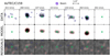 |
Fig. 2. Comparison between data and 3DBAROLO best-fit model for AzTEC/C159. Top row: seven representative channel maps showing the [C II] 158-μm emission of AzTEC/C159 (low spectral resolution data cube; see Table 3). The contours are at −2, 2, 4, and 8 times the rms noise per channel (σ). Line-of-sight velocities with respect to systemic velocity (set at v = 0) are shown on top of each channel map. Middle row: channel maps of the axi-symmetric best-fit model obtained with 3DBAROLO; the contours are at the same levels as in the data. Bottom row: residuals (data minus model); pink contours are negative (−2σ), and light blue contours are positive (+2σ). In all panels, the green cross shows the dynamical centre, whose coordinates are given in Table 1. |
We finally ran 3DBAROLO keeping all the geometrical parameters and the systemic frequency fixed and simultaneously fitting the rotation velocity and the velocity dispersion of the gas. The surface density of the model is derived directly from the data as an azimuthal average within the annuli. In Fig. 1, we overlay the contours from our best-fit model cube on the p-v diagrams along the major and minor axes, while in Fig. 2 we show some representative channel maps of the data and model as well as the resulting residuals. It is clear from these comparisons that the fit is of very high quality and that the [C II] emission of AzTEC/C159 is reproduced very well by a disc in differential rotation.
3.2. Rotation curve analysis of AzTEC/C159
The values of rotation velocity and velocity dispersions in the two rings are shown in Fig. 3. In order to calculate the errors, 3DBAROLO performs a Monte Carlo sampling of the parameter space around the best-fit value. However, this does not take into account the uncertainties on parameters that have been fixed in the fit. As mentioned, the main uncertainty for AzTEC/C159 is given by the relatively low inclination angle of the disc. Therefore, we calculated the errors by re-running 3DBAROLO and fixing the inclination first to 30° (the upper bound in rotation velocity) and then to 50° (the lower bound). The resulting errors were summed in quadrature with the nominal (Monte Carlo) errors of the fit, which in any case are subdominant. For consistency, we used the same method to estimate the errors in the velocity dispersion.
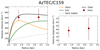 |
Fig. 3. Best-fit rotation velocities and velocity dispersions of AzTEC/C159. Left panel: rotation velocities of the two annuli in which we decomposed the disc of AzTEC/C159. The orange and green curves show the contribution of stars and gas, respectively, modelled as exponential discs, the dashed grey curve shows that of a dark matter halo modelled as an NFW profile, and the black curve is the sum of all components. This comparison is illustrative and not fitted to the data points. Right panel: gas velocity dispersion in the two annuli obtained using the low spectral resolution data cube (see Sect. 3.5 for the high-resolution values). |
The two annuli return rotation velocities and velocity dispersions consistent with each other. Regarding the rotation velocity, this result hints at a flat rotation curve, although we caution that our two rings are not fully independent and that it is difficult to draw conclusions about the precise shape of the curve. The resulting rotation velocity, averaged between that of the two rings, is very high,  , consistent with the value found by Jones et al. (2017) if we use their inclination of 30°. From this rotation velocity (assuming it is equal to the circular speed vc), we can derive a dynamical mass2 out to the outer measured point of
  . As an illustration, in Fig. 3 (left panel) we show the contribution of two razor-thin exponential discs (Freeman 1970) to represent the contribution of stars and gas. For the stars, we used the FIR effective radius of
  determined at ≈870 μm (rest-frame ≈160 μm) by Gómez-Guijarro et al. (2018). We converted this FIR radius to an approximate rest-frame optical effective radius using a multiplicative factor of 1.4 (Fujimoto et al. 2017). From this we derived the exponential scale-length Rd using the standard conversion Rd = Re/1.678. Such a stellar component, with the measured stellar mass3 of 4.5 × 10¹⁰ M⊙ (Table 1), gives a contribution that appears to reproduce the high rotation velocity close to the centre of the galaxy well (first point of the rotation curve).
We derived the exponential scale-length of the gas disc from the [C II] zeroth moment map using Galfit (Peng et al. 2010a) and obtained Rgas = 1.3 ± 0.4 kpc. This, combined with a gas mass of 1.5 × 10¹¹ M⊙ (Jiménez-Andrade et al. 2018), gives the contribution shown by the green curve in Fig. 3. For the dark matter halo, we assumed a Navarro-Frenk-White (NFW) profile (Navarro et al. 1996) with a concentration c200 = 3.4, which is appropriate for halos of very different masses at these redshifts (Dutton & Macciò 2014), and a mass M200 = 2 × 10¹² M⊙ (e.g. Rizzo et al. 2020). Despite the large mass, it is clear that the dark matter remains subdominant (see dashed grey curve) and only completely unrealistic values of M200 > 1014 M⊙ would give a contribution in these inner regions of the galaxy comparable to the baryons. Using alternative profiles for the dark matter halo (such as the pseudo-isothermal profile) also makes only a negligible difference. Unfortunately, the low angular resolution of our data does not allow for a full decomposition of the rotation curve (Cimatti et al. 2019); however, we can derive two important indications from this analysis. First, it is clear that the dynamical properties of AzTEC/C159 show that we are dealing with an extremely baryon-dominated object (the baryon-to-dark mass ratio at the outer measured point is ≈10). Second, the available estimates of masses and sizes of both the stellar and gaseous discs are in good agreement with our inferred dynamical properties.
The velocity dispersion in Fig. 3 (right panel) shows large error bars but favours values of the order of a few tens of km s−1. We note that this value is close to the velocity resolution of our data, meaning that the velocity dispersion cannot be reliably measured by 3DBAROLO. Clearly, this points to a strongly rotation-dominated system, with values of V/σ ≳ 10. We return to this point in Sect. 3.5.
3.3. 3D kinematic fit of J1000+0234
In this section, we describe the data of our second galaxy, J1000+0234, and the kinematic fit that we performed with 3DBAROLO to obtain the rotation velocity and the velocity dispersion. A number of descriptions are similar to those in Sect. 3.1 and are thus only briefly repeated.
The total-flux map of the [C II] 158-μm emission of J1000+0234 is shown in the top (left and middle) panels of Fig. 4. Contrary to AzTEC/C159, this galaxy appears very elongated in [C II] emission, with an axis ratio of roughly two despite the low angular resolution. It should be noted that the ALMA beam is elongated in the opposite direction. Thus, the [C II] morphology points to a highly inclined (nearly edge-on) galaxy. As mentioned, HST shows a complex structure characterised by two emission regions, one of which overlaps with the [C II] emission although not with the peak of this emission. This again can be due to dust absorption, and, as a consequence, the morphology of the stellar component in J1000+0234 is largely unconstrained.
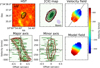 |
Fig. 4. [C II] 158-μm observations and modelling of J1000+0234. Top left panel: HST WFC3 F160W image with the [C II] 158-μm total-flux map contours overlaid. Top middle panel: total-flux map (green shapes and black contours) of the [C II] emission; the lowest contour is at about 3 times the rms noise in this map, and the other contours are at 2, 4, and 8 times this level. In red we show the outer contour of the total-flux map of the best-fit model obtained with 3DBAROLO (convoluted with the observational beam, shown in the bottom right corner). Top right panel: velocity (weighted-mean) field of the [C II] 158-μm line. Bottom left panel: position-velocity diagram along the kinematic major axis of the galaxy (grey line overlaid on the velocity field); the data are in green shades and contours, while the 3DBAROLO model is in red contours. Contour levels are at −2, 2, 4, and 8 times the rms noise per channel. Bottom centre panel: position-velocity diagram along the kinematic minor axis of the galaxy displayed analogously to the major-axis plot. Bottom right panel: velocity (weighted-mean) field of the best-fit 3DBAROLO model. |
The velocity field of J1000+0234 (top right panel in Fig. 4) shows a regular gradient along the elongation of the emission, suggesting rotation. This is corroborated by the p-v diagram along the major axis of the emission shown in the bottom left panel. As for AzTEC/C159, we see here the typical pattern of a rotating disc observed at low angular resolution (Di Teodoro & Fraternali 2015). The p-v diagram along the minor axis again shows a very broad emission indicative of a very fast rising rotation curve combined with a strong beam smearing effect. As already noted by Schinnerer et al. (2008) for CO, the global extent of the emission line exceeds 1000 km s−1. In the following, we show that this is the result of the very fast (differential) rotation of the gaseous disc.
The fitting of J1000+0234 with 3DBAROLO is somewhat easier than that of AzTEC/C159 given the high inclination of the disc, which makes the final value of the rotation velocity very robust. Here, we have assumed an inclination of the disc of 75°. This value was obtained using trial and error and by comparing the model total-flux map with that of the data; the red contour in the top middle panel of Fig. 4 shows that a model with this inclination reproduces the [C II] outer contour very well. The calculation of the residuals between total-flux maps of 3DBAROLO models with varying inclinations and the observed total-flux map returns a minimum at 73°, confirming the trial-and-error value.
The other parameters of the disc were determined in a way analogous to AzTEC/C159. Small adjustments with respect to 3DBAROLO estimates were performed after visual inspection, but they were of the order of, or smaller than, the quoted errors (Table 2). The systemic frequency is somewhat uncertain because the emission is so broad that it reaches the edge of the ALMA band. However, the shape of the channel maps (Fig. 5) and of the p-v diagrams in Fig. 4 indicate that the disc emission beyond the edge of the band must be very limited (at most a channel or two, assuming symmetry between the approaching and receding sides). The kinematic centre that we found is 0.4″ away from the peak of the CO (J = 4 → 3) emission in Schinnerer et al. (2008), which was obtained from data with a resolution of roughly 2″.
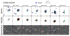 |
Fig. 5. Comparison between data and 3DBAROLO best-fit model for J1000+0234. Top row: seven representative channel maps showing the [C II] 158-μm emission of J1000+0234. The contours are at −2, 2, 4, and 8 times the rms noise per channel (σ). Line-of-sight velocities with respect to the systemic velocity (set at v = 0) are shown on top of each channel map. Middle row: channel maps of the axi-symmetric best-fit model obtained with 3DBAROLO; the contours are at the same levels as in the data. Bottom row: residuals (data−model); pink contours are negative (−2σ), and light blue contours are positive (+2σ). In all panels, the green cross shows the dynamical centre, whose coordinates are given in Table 2. |
Once all the geometrical parameters were fixed (Table 2), we ran 3DBAROLO to simultaneously fit rotation velocity and velocity dispersion. Given the size of the galaxy along the major axis and the orientation of the beam, we used three adjacent annuli that were each 0.2″ wide. Regarding AzTEC/C159, this is a small oversampling of our data (see Table 4) that makes the three values that we obtained not fully independent. However, it allows us to have an indication of the shape of the rotation curve in this galaxy. The emission of the best-fit model is shown overlaid on the p-v diagrams in Fig. 4. In Fig. 5, we show the comparison between seven representative channel maps of the [C II] emission of J1000+0234 and our best-fit model. The bottom panels show the residuals of the emission: data−model. It is clear from these comparisons that the [C II] 158-μm emission of J1000+0234 is reproduced very well by an axi-symmetric disc in differential rotation.
3.4. Rotation curve analysis of J1000+0234
Given the high inclination of the disc of J1000+0234, the obtained rotation velocities are quite robust and the errors are significantly smaller than for AzTEC/C159. Figure 6 (left panel) shows the measured points and the errors obtained as sums in quadrature of the nominal errors from the fit and the generous variation in inclination of ±10°. The rotation curve appears quite flat as the velocities of all the rings are compatible. We recall that, due to our slight oversampling, these points are not fully independent from one another; however, the fact that the first and the third ring are at the same rotation velocity is a good indication of a flat curve. The average rotation velocity across the disc is very high, vrot = 538±40 km s−1, leading to a dynamical mass within the last measured point of (2.3 ± 0.3) × 1011 M⊙.
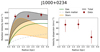 |
Fig. 6. Best-fit rotation velocities and velocity dispersions of J1000+0234. Left panel: rotation velocities measured in J1000+0234 (red points) compared to the contributions of different matter components. This comparison is illustrative and not fitted to the data points. Orange lines and shades indicate the contribution of the stellar component given the two estimates of stellar mass present in the literature. The solid green curve indicates the contribution of the gas disc, which is assumed exponential and is derived from the [C II] 158-μm distribution. The dashed grey curve indicates the contribution of a dark matter halo given by an NFW profile with a virial mass of M200 = 2 × 10¹² M⊙. The black lines and shade indicate the total contribution of all components. Right panel: [C II] velocity dispersion measured in J1000+0234. |
As for AzTEC/C159, the presence of only three (and not fully independent) points does not allow for a full decomposition of the rotation curve (Cimatti et al. 2019). However, calculating the contributions of the various matter components is highly instructive. As mentioned, the stellar mass of J1000+0234 is largely unconstrained as there are two very different determinations in the literature. The stellar size cannot be determined directly since the source is heavily absorbed in the HST bands and is essentially unresolved by Spitzer at near-infrared (NIR) wavelengths (Smolčić et al. 2015). Therefore, as for AzTEC/C159, we used the FIR effective radius Re = 700 pc (Gómez-Guijarro et al. 2018), multiplied by 1.4 to convert it to an approximate optical rest-frame effective radius (Fujimoto et al. 2017) and divided by 1.678 to get an exponential scale-length Rd. This leads, for the two values of stellar masses, to the shaded orange area in Fig. 6. Thus, the inner point of the rotation curve can be reproduced by a stellar component if the stellar mass is on the high side of the range (Table 2).
For the gaseous disc, we used the [C II] 158-μm zeroth moment map to obtain an exponential scale-length Rgas = 1.5 ± 0.2 kpc from Galfit (Peng et al. 2010a). We calculated the contribution to the rotation curve of this component and found that, in order to reproduce the outer point at 3.3 kpc, the gas mass has to be significantly larger than the estimate from Schinnerer et al. (2008) of 2.8 × 10¹⁰ M⊙. This estimate was obtained from CO (J = 4 → 3) using a low αCO factor (0.8 M⊙(Kkm s−1 pc2)−1) that is likely not appropriate for an object such as J1000+0234 (Papadopoulos et al. 2012; Jiménez-Andrade et al. 2018). The top panel of Fig. 6 shows the contribution of a gaseous disc with a mass Mgas = 1.5 × 10¹¹ M⊙. We note that, as for AzTEC/C159, this is the total mass of the extrapolated exponential profile, which we used to determine the central surface density as  . However, given that the scale-length is quite large (Rgas = 1.5 kpc), only ≈73% of this mass (≈1.1 × 10¹¹ M⊙) resides within the extent of the [CII] disc: Rext ≈ 0.6″ ≈ 4 kpc. This mass leads to a ratio between [C II] luminosity and gas mass (both in standard units), α[C II] ≈ 8 (using the luminosity L′ in Carilli & Walter 2013), in agreement with values determined for other high-z starbursts (Gullberg et al. 2018). We also note that J1000+0234 and AzTEC/C159 having similar gas masses is in line with their having similar dust masses (Smolčić et al. 2015) and [C II] fluxes (Tables 1 and 2). All these considerations indicate that the gas mass of J1000+0234 is likely ≈1 × 10¹¹ M⊙.
The top panel of Fig. 6 also shows the contribution from the dark matter halo and the combination of all components (black lines and the grey band). For the dark matter halo, we have assumed an NFW profile (Navarro et al. 1996) with a concentration c200 = 3.4 and a mass M200 = 2 × 10¹² M⊙ (see Sect. 3.2). As for AzTEC/C159, the dark matter is almost negligible in these inner regions of the galaxy for any realistic choice of the virial mass. We can conclude that the inner kiloparsecs of J1000+0234 probed by our data are fully baryon-dominated, with the gas mass slightly larger than the stellar mass.
The right panel of Fig. 6 shows the [C II] velocity dispersion in J1000+0234 that we derived with 3DBAROLO. The values are, as for AzTEC/C159, quite low, leading to a V/σ of the order of ten. However, being the galaxy at high inclination, these velocity dispersions should be considered to be more uncertain than those of AzTEC/C159. They could in fact be overestimated as some line broadening can occur, along the line of sight, because of projection effects. This effect is difficult to account for, but it becomes less important in the outer disc; therefore, a realistic value of the velocity dispersion is potentially given by the last ring at ≈ 30 km s−1. In the following, we attempt to give a better quantification of the velocity dispersion using data at high spectral resolution and focusing on AzTEC/C159.
3.5. The [C II] velocity dispersion in AzTEC/C159
The [C II] disc of AzTEC/C159 is seen at a relatively low inclination with respect to the line of sight. This makes its rotation velocity quite sensitive to small variations of inclination and therefore relatively uncertain (see error bars in Fig. 3). However, the gas velocity dispersion is, in these situations, robustly measured. In order to obtain such a measure, we used 3DBAROLO, which allows us to properly account for beam smearing (see Sect. 3.3). We obtained values of about 40 km s−1 though with very large uncertainties due to the fact that our data cube (Table 3) has a velocity resolution of 27 km s−1, which makes it very difficult to reliably measure dispersions around that value.
We thus produced a high spectral resolution data cube with a channel separation of 10.3 km s−1. This reduces the S/N per channel but still allows us to obtain a reliable kinematic fit. Figure 7 shows the emission in this data cube through p-v diagrams along and perpendicular to the major axis, analogous to those shown in Fig. 1. The pattern of rotation is very clear, as in the low spectral resolution data cube, but the emission tends to break up in the middle channels close to systemic velocity due to the low S/N. The quality of the fit obtained with 3DBAROLO (shown in red contours) also appears very good at these high spectral resolutions. This fit returns an extremely low velocity dispersion, σgas = 16 ± 13 km s−1 (averaging the two rings), again of the order of the channel resolution. These low values of velocity dispersion are robust over any initial guesses for the fit, which we made to vary between σguess = 10 km s−1 and σguess = 300 km s−1. The values of the rotation velocity obtained with this high spectral resolution data cube are fully compatible with those presented in Sect. 3.1.
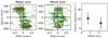 |
Fig. 7. Data and best-fit 3DBAROLO model of AzTEC/C159 at high spectral resolution. Left panel: position-velocity diagram along the kinematic major axis of AzTEC/C159 (see Fig. 1) obtained using the high spectral resolution data cube (Table 3). The [C II] 158-μm emission in the data is in green shades and contours, while the 3DBAROLO model is in red contours. Contour levels are at −2, 2, 4, and 8 times the rms noise per channel. Centre panel: position-velocity diagram along the kinematic minor axis displayed analogously to the major-axis plot. Right panel: [C II] velocity dispersion obtained from the high spectral resolution data cube. |
To further test the reliability of the above fit, we ran 3DBAROLO with the spacepar keyword turned on. This keyword allows the user to explore the full parameter space of two parameters by calculating the residual (|model−data|) in a grid with arbitrary spacing. We used as free parameters the rotation velocity (vrot) and the velocity dispersion (σgas) and explored a large portion of the space around the best-fit values determined above. This exploration was done for the two rings separately, and the final result is shown in Fig. 8. There we see the values of the residual for any pair of vrot and σgas in a range of about 200 km s−1 in each direction. It is clear that the exploration of both rings shows a well-defined absolute minimum, and there is no sign of a secondary minimum. The contours show regions where the residuals are at two, five, and ten times the absolute minimum. The favoured models are clearly at vrot ≈ 500 km s−1 and σgas ≲ 20 km s−1, in agreement with the best-fit values determined above.
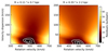 |
Fig. 8. Exploration of the large-scale parameter space of the residuals between the data and the models, calculated as the absolute value of model minus data; as data, we used the high spectral resolution data cube of AzTEC/C159, and each model is built with a different pair of vrot and σgas, with the other parameters kept fixed. Left panel: residuals in the inner ring; contours show levels where the residuals exceed 2, 5, and 10 times the minimum value, respectively. Right panel: same, but for the outer ring. |
We also ran kinematic fits of our two galaxies using Galpak3D (Bouché et al. 2015). We found values for the rotation velocities, the velocity dispersions, and the inclinations that are fully consistent, within the errors, with the 3DBAROLO runs.
4. Discussion
In the previous sections, we have seen the results of 3D kinematic fits of the ALMA [C II] 158-μm data cubes of two starburst galaxies at z ≈ 4.5 obtained with the software 3DBAROLO. These two galaxies, which show a number of similarities with each other based on their photometric properties (see Tables 1 and 2), also appear very similar in terms of dynamical properties as estimated from the [C II] gas kinematics. The general picture that we obtain is of very fast rotating gas discs with relatively low velocity dispersion as well as V/σ values comparable to z = 0 spiral galaxies. In the following sections, we discuss the reliability of our results as well as possible evolution scenarios for these galaxies that emerge from our dynamical analysis.
4.1. Determining if velocity gradients can indicate anything other than rotation
In Sects. 3.1 and 3.3, we have seen how well a model of a rotating disc can reproduce the emission in the data cubes of both AzTEC/C159 and J1000+0234. We wanted to determine whether this is a unique possibility or if there are other configurations that can give a similar pattern. In general, a velocity gradient seen at low angular resolution should be taken with caution. At high angular resolution, a rotating disc gives an extremely distinctive pattern that leaves no room for alternative interpretations (Swaters et al. 2002; Fraternali et al. 2002; Walter et al. 2008). However, velocity gradients can also be evidence of outflows (Martini et al. 2018), mergers (Sweet et al. 2019), or, potentially, gas inflow. Thus, in particular at high redshift, one should question whether or not these phenomena can play a role.
However, a careful inspection of our data, looking both at the channel maps and the p-v diagrams, reveals the distinctive aspect of our velocity gradients. The channel maps of both galaxies show a remarkably clear pattern of a rotating disc with a flat rotation curve as the emission accumulates at the extreme (approaching and receding) channels (see panels 2 and 6, from left to right, in Figs. 2 and 5), becoming dimmer instead close to systemic velocity. This is also plainly visible in the p-v diagrams in Figs. 1 and 4 and especially in Fig. 7, where we also see, by looking at the model contours, that a rotating disc with a flat rotation curve predicts precisely this pattern. Moreover, the relatively low inclination of AzTEC/C159 allows us to admire another distinctive feature of rotating discs: the ‘butterfly’ opening of the channel maps close to the systemic velocity (Fig. 2). Finally, both galaxies show a velocity gradient nicely aligned with the elongation of the [C II] emission (i.e. the morphological and kinematic axes coincide), a further feature of rotating discs. We conclude that there is no reason to doubt that the structures that we are observing in these two galaxies are rotating discs at z ≈ 4.5. This is in line with recent results obtained for similar galaxies at slightly higher angular resolution (Neeleman et al. 2020; Lelli et al. 2021) and with the help of gravitational lensing (Rizzo et al. 2020).
4.2. Understanding the low gas turbulence in AzTEC/C159
The gas velocity dispersion of AzTEC/C159 (Sect. 3.5) is significantly lower relative to values determined by other authors for similar systems (e.g. Hodge et al. 2012; Carniani et al. 2013) as well as expectations from numerical simulations (Zolotov et al. 2015; Pillepich et al. 2019, but see Kohandel et al. 2020). From the observational side, our result is a combination of two improvements with respect to other works as (1) we used 3DBAROLO to fully account for the beam smearing and (2) we used a data cube at very high spectral resolution (≈ 10 km s−1). From the theoretical side, it is useful to estimate whether such a low dispersion can be expected from simple arguments.
We assumed that the velocity dispersion that we measure for the [C II] is representative of the cold molecular ISM of AzTEC/C159, which has a total mass Mgas ≃ 1.5 × 10¹¹ M⊙ (Table 1). Given the SFR of this galaxy of 740 M⊙ yr−1, one would expect a supernova rate (SNR) of SNR ≈ 7 yr−1, assuming a standard initial mass function. The energy input from supernovae that can feed turbulence is then
 (1)
(1)
where we have taken the standard total energy per supernova of 1051 erg and an efficiency of transferring kinetic energy to the ISM of 10% (Chevalier 1974; Ohlin et al. 2019). The total turbulent (kinetic) energy of the gas disc of AzTEC/C159 can simply be estimated as
 (2)
(2)
where σgas is the gas velocity dispersion that we can expect to measure and the factor 3 comes from the fact that this dispersion is measured along the line of sight. Turbulence is dissipated on timescales of τ ≈ h/σgas (Mac Low 1999), where h is the scale-height of the disc that unfortunately is unknown and we assume to be in the range h = 100 − 500 pc. To maintain turbulence at the observed value, supernovae must provide energy at the rate Ėturb = Eturb/τ. By equating this energy input (see also Rizzo et al. 2020) with the one available in Eq. (1), we can estimate a gas velocity dispersion of
 (3)
(3)
and, considering the range in h and the errors in the SNR (i.e. the SFR) and MH_2, we obtain that σgas is in the range 22–50 km s−1 for an efficiency η = 0.1. In conclusion, the values of gas velocity dispersion that we have measured are on the low side of this estimate. They could point to an overestimate of the SFR or a relatively low efficiency of energy transfer to the ISM (of a few percent). Recent similar estimates, carried out in local galaxies, indeed show that only a few percent of the supernova energy goes to the feeding of the ISM turbulence (Bacchini et al. 2020).
In this context, it is important to point out that a velocity dispersion of ≈ 20−30 km s−1, although lower than other literature determinations, is still quite large considering that the [C II] 158-μm line is tracing a rather cold component of the ISM. In local galaxies, molecular gas has typical velocity dispersions of ≈ 5 km s−1 (Marasco et al. 2017; Koch et al. 2019; Bacchini et al. 2020), while atomic neutral gas has ≈ 10 km s−1 (e.g. Tamburro et al. 2009; Bacchini et al. 2019). Thus the gas velocity dispersions that we are measuring in our high-z starburst galaxies are higher than those of z = 0 discs, but not exceedingly so.
In the above analysis, we have focused on AzTEC/C159, which gives the most reliable measure of the velocity dispersion. The high inclination of J1000+0234 is, instead, likely broadening the line profiles, an effect that 3DBAROLO can only partially compensate for (Di Teodoro & Fraternali 2015). Moreover, the large uncertainties in SFR and gas mass (Table 2) would make the above calculation not very predictive since Eq. (3) returns values in the range 14−100 km s−1 for η = 0.1.
4.3. Evolution of high-z starbursts
Massive starburst galaxies at z ≈ 4 are believed to be the progenitors of massive ETGs (e.g. Toft et al. 2014). This expectation is mostly based on the extremely high SFRs combined with high stellar and gas masses. The depletion time of these galaxies is typically significantly less than 1 Gyr, pointing to the possibility that the whole stellar population can be formed before, say, z ≈ 2 − 3 and that the galaxy will eventually evolve passively and through dry mergers. Massive ETGs at z ≈ 2 are indeed observed, with stellar masses comparable to local ETGs and rather compact sizes (e.g. Cimatti et al. 2008; Cappellari 2016). Our results allow us to test this evolutionary hypothesis dynamically.
The kinematics and dynamics of local ETGs are typically studied using stellar absorption lines (Thomas et al. 2007; Cappellari et al. 2013; Corsini et al. 2017; Zhu et al. 2018). However, some ETGs have cold gas that allows a variety of kinematic studies (Davis et al. 2011a; Serra et al. 2014; Shelest & Lelli 2020). In particular, it is relatively common for ETGs (roughly 20% of cases) to have central compact discs of molecular gas with typical sizes of ∼1 kpc that allow us to probe the gravitational potential in the inner regions (Davis et al. 2013). These discs often show regular rotation patterns displayed by the global profiles (Davis et al. 2011b) and by resolved observations (Young 2005; North et al. 2019). It has been shown (Davis et al. 2016) that these CO discs fulfil the ETG analogue of a stellar-mass Tully-Fisher relation (Tully & Fisher 1977). We show this relation in Fig. 9 for the sample of galaxies in Davis et al. (2016). We note that the velocities were slightly revised due to better determinations of the inclinations of the discs (Davis, priv. comm.) and that the masses are determined from the K-band luminosity assuming a mass-to-light ratio M/L = 0.5 M⊙/L⊙, K. In the same figure, we also include our two high-z starbursts. For their rotation velocities, we used the values that we obtained from their [C II] discs, which are similar in size to the CO discs in local ETGs. For the stellar masses, we used the estimated stellar mass (empty symbols), and we estimated their ‘final’ mass by assuming that they will convert all their gas into stars (filled symbols). For J1000+0234, we used an average stellar mass between the two estimates (Table 2) and the gas mass that we determined through the rotation curve decomposition (Sect. 3.4). After the conversion of gas into stars, our two high-z starbursts appear to fully overlap with the local ETGs.
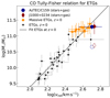 |
Fig. 9. Stellar-mass Tully-Fisher (analogue) relation for ETGs at z = 0 from Davis et al. (2016) compared with the positions of our starburst galaxies at z ≈ 4.5. In the local ETGs, the rotational speed is derived from the inner CO discs, while in our galaxies it is obtained from the [C II] line. The empty symbols show the positions of our galaxies based on the observed stellar mass, while the filled symbols show their positions assuming that all the observed gas mass is converted into stars. |
A number of considerations can be drawn from the comparison presented in Fig. 9. First, it appears that the inner potential well of our galaxies at z ≈ 4.5, quantified by their circular speed, is indeed comparable with that of the most massive ETGs that we observe today. Second, the conversion of the gas mass into stellar mass, which is expected to occur in a few hundred megayears (depletion time), can make these galaxies lie in the same scaling relation as massive local ETGs. We note that although we are unable to give a precise quantification of the stellar effective radius of our galaxies, it is likely that they will be smaller than those of local ETGs that have the same stellar mass (van der Wel et al. 2014; Cappellari 2016), as was shown by Gómez-Guijarro et al. (2018) using the FIR sizes. Thus, the effective radius of these galaxies will likely grow with time, which will also have potential consequences on the precise value of the inner circular speed. However, in general terms, we can envisage a scenario in which our galaxies convert all their gas into stars, go through a quenching phase (e.g. Peng et al. 2010b), and then evolve passively and through mergers to be observed today at the massive end of the ETGs.
The most puzzling aspect of the above scenario is the extremely fast rotation velocity that we measured. On the one hand, there is no surprise that the circular speed in these high-z starbursts is 500 km s−1 because it is also the case for the most massive local ETGs. On the other hand, however, we observe a very large mass (∼1011 M⊙) of gas rotating at that speed; when this gas is turned into stars, it is conceivable to imagine that these stars will rotate very fast. Thus, we should end up with an extremely massive and compact rotation-supported stellar disc. Stellar discs with similar properties have been found in a some gravitationally lensed galaxies at z ≈ 2 − 2.5 (Newman et al. 2015; Toft et al. 2017), and it is possible that the two starbursts studied in this paper are progenitors of this kind of object. However, it is important to note that the V/σ values of the z ≈ 2 stellar discs are much smaller than what we measured in our z ≈ 4.5 starbursts.
In the local Universe, stellar discs rotating at v > 300 km s−1 are extraordinarily rare (Posti et al. 2018; Ogle et al. 2019), and it is unlikely that they are the end point of the evolution of high-z starburst galaxies, given the reasons mentioned above. Therefore, it appears necessary that the stars that form in these high-z fast rotating and cold discs redistribute into a pressure-supported system analogous to a slow rotator ETG (Cappellari 2016). A phenomenon that can help in this direction is a major merger or a large number of minor mergers (see discussion in Rizzo et al. 2020). However, it is tempting to also consider the possibility of global disc instabilities (e.g. Ostriker & Peebles 1973; Sellwood et al. 2013). We leave the exploration of these possibilities to future works.
5. Conclusions
We have studied the kinematics of two starburst galaxies at z ≈ 4.5 (AzTEC/C159 and J1000+0234) using the [C II] 158-μm emission line observed with ALMA at an angular resolution of ≈0.3″, which corresponds to ≈2 kpc. We have modelled the [C II] emission using the code 3DBAROLO, which fits a tilted-ring galaxy model in 3D space by producing artificial data cubes that include all observational biases. In particular, 3DBAROLO is capable of accounting for the effect of beam smearing, which is particularly severe with data at these angular resolutions. The main results of this work are as follows.
-
The [C II] 158-μm emission of our two galaxies is perfectly reproduced by models of gas discs in regular (differential) rotation.
-
The best-fit rotation velocities are
 and 538±40 km s−1 for AzTEC/C159 and J1000+0234, respectively. The errors in the former galaxy are larger due to the relatively low inclination of the disc.
 -
We show that the masses of the stellar and gaseous disc components needed to reproduce these rotation velocities are compatible with the literature values for AzTEC/C159, while J1000+0234 requires higher values of ≈1011 M⊙. Both galaxies are strongly baryon-dominated in the probed regions (the inner few kiloparsecs) with a negligible dark matter contribution.
-
The best-fit gas (intrinsic) velocity dispersions are at least a factor of ten lower than the rotation velocities. As these values are of the order of the velocity resolution of our initial data cube, we repeated the kinematic fit for AzTEC/C159 in a data cube with a spectral resolution of 10 km s−1, finding a best-fit velocity dispersion σgas = 16±13 km s−1, which leads to V/σ ≳ 20.
-
We showed that the surprisingly low velocity dispersion of AzTEC/C159 can be compatible with turbulence fed by supernovae with an efficiency η ≲ 10%.
-
Our galaxies appear to have potential wells (demonstrated by the measured circular speeds) that are very similar to those of local massive ETGs. A comparison of their positions in the ETG analogue of the stellar-mass Tully-Fisher relation, obtained from the rotation of CO discs in ETGs, reveals an almost perfect overlap provided that all the observed gas in our high-z galaxies is converted into stars.
In conclusion, our results provide dynamical support to the idea that high-z starbursts are progenitors of local ETGs. If the galaxies already have extremely deep potential wells at z ≈ 4.5, the conversion of gas into stars, combined with the subsequent quenching of star formation, should produce objects that can then both structurally and dynamically evolve passively into ETGs. The puzzle that remains unsolved concerns the transformation of a highly rotation-supported system into a likely slow rotator ETG.
We note that, given that we are using a mask, the noise is not constant across the total-flux map, although we have verified that the variations along the outer contours shown in Figs. 1 and 4 are small (less than 20%). For more details about the S/N levels of outer contours in these types of maps, see Iorio et al. (2017).
This is calculated with the standard formula  (with Rout the radius of the outer ring), which gives an estimate that is correct within 10% for exponential discs at radii R ≳ 2.2Rd, i.e. around and beyond the peak of their contribution (Binney & Tremaine 2008). The errors in the dynamical mass are calculated considering the 1-σ uncertainty in vc.
This stellar mass, as well as the gas mass below, are used to derive the central surface brightness of the exponential disc as  .
.
Acknowledgments
We thank Timothy Davis for providing his data on local ETGs, Eric Emsellem for stimulating discussions and Ian Smail for helpful comments. We also thank an anonymous referee for an useful and constructive report. FF acknowledges support from the Friedrich Wilhelm Bessel Research Award Programme of the Alexander von Humboldt Foundation. AK and BM acknowledge support by the Collaborative Research Council 956, sub-project A1, funded by the Deutsche Forschungsgemeinschaft (DFG). C.G.G. acknowledges support from the European Research Council (ERC) Consolidator Grant funding scheme (project ConTExt, grant number: 648179). This work makes use of the following ALMA data: 2012.1.00978.S and 2015.1.01564.S. ALMA is a partnership of ESO (representing its member states), NSF (USA), and NINS (Japan), together with NRC (Canada), NSC and ASIAA (Taiwan), and KASI (Republic of Korea), in cooperation with the Republic of Chile. The Joint ALMA Observatory is operated by ESO, AUI/NRAO, and NAOJ.
References
- Aguirre, P., Baker, A. J., Menanteau, F., Lutz, D., & Tacconi, L. J. 2013, ApJ, 768, 164 [NASA ADS] [CrossRef] [Google Scholar]
- Aretxaga, I., Wilson, G. W., Aguilar, E., et al. 2011, MNRAS, 415, 3831 [Google Scholar]
- Bacchini, C., Fraternali, F., Iorio, G., & Pezzulli, G. 2019, A&A, 622, A64 [NASA ADS] [CrossRef] [EDP Sciences] [Google Scholar]
- Bacchini, C., Fraternali, F., Iorio, G., et al. 2020, A&A, 641, A70 [CrossRef] [EDP Sciences] [Google Scholar]
- Battaglia, G., Fraternali, F., Oosterloo, T., & Sancisi, R. 2006, A&A, 447, 49 [NASA ADS] [CrossRef] [EDP Sciences] [Google Scholar]
- Binney, J., & Tremaine, S. 2008, Galactic Dynamics (Second Edition) [Google Scholar]
- Birkin, J. E., Weiss, A., Wardlow, J. L., et al. 2021, MNRAS, 501, 3926 [Google Scholar]
- Bouché, N., Carfantan, H., Schroetter, I., Michel-Dansac, L., & Contini, T. 2015, AJ, 150, 92 [NASA ADS] [CrossRef] [Google Scholar]
- Cantalupo, S., Pezzulli, G., Lilly, S. J., et al. 2019, MNRAS, 483, 5188 [NASA ADS] [CrossRef] [Google Scholar]
- Capak, P., Carilli, C. L., Lee, N., et al. 2008, ApJ, 681, L53 [Google Scholar]
- Cappellari, M. 2016, ARA&A, 54, 597 [NASA ADS] [CrossRef] [Google Scholar]
- Cappellari, M., Scott, N., Alatalo, K., et al. 2013, MNRAS, 432, 1709 [NASA ADS] [CrossRef] [Google Scholar]
- Caputi, K. I., Deshmukh, S., Ashby, M. L. N., et al. 2017, ApJ, 849, 45 [NASA ADS] [CrossRef] [Google Scholar]
- Carilli, C. L., & Walter, F. 2013, ARA&A, 51, 105 [Google Scholar]
- Carniani, S., Marconi, A., Biggs, A., et al. 2013, A&A, 559, A29 [NASA ADS] [CrossRef] [EDP Sciences] [Google Scholar]
- Casey, C. M., Narayanan, D., & Cooray, A. 2014, Phys. Rep., 541, 45 [Google Scholar]
- Chevalier, R. A. 1974, ApJ, 188, 501 [NASA ADS] [CrossRef] [Google Scholar]
- Cimatti, A., Cassata, P., Pozzetti, L., et al. 2008, A&A, 482, 21 [NASA ADS] [CrossRef] [EDP Sciences] [Google Scholar]
- Cimatti, A., Fraternali, F., & Nipoti, C. 2019, Introduction to Galaxy Formation and Evolution: From Primordial Gas to Present-Day Galaxies [Google Scholar]
- Corsini, E. M., Wegner, G. A., Thomas, J., Saglia, R. P., & Bender, R. 2017, MNRAS, 466, 974 [NASA ADS] [CrossRef] [Google Scholar]
- da Cunha, E., Walter, F., Smail, I. R., et al. 2015, ApJ, 806, 110 [Google Scholar]
- Davis, T. A., Alatalo, K., Sarzi, M., et al. 2011a, MNRAS, 417, 882 [NASA ADS] [CrossRef] [Google Scholar]
- Davis, T. A., Bureau, M., Young, L. M., et al. 2011b, MNRAS, 414, 968 [NASA ADS] [CrossRef] [Google Scholar]
- Davis, T. A., Alatalo, K., Bureau, M., et al. 2013, MNRAS, 429, 534 [NASA ADS] [CrossRef] [Google Scholar]
- Davis, T. A., Greene, J., Ma, C.-P., et al. 2016, MNRAS, 455, 214 [NASA ADS] [CrossRef] [Google Scholar]
- de Blok, W. J. G., Walter, F., Brinks, E., et al. 2008, AJ, 136, 2648 [NASA ADS] [CrossRef] [Google Scholar]
- De Breuck, C., Williams, R. J., Swinbank, M., et al. 2014, A&A, 565, A59 [NASA ADS] [CrossRef] [EDP Sciences] [Google Scholar]
- Di Teodoro, E. M., & Fraternali, F. 2015, MNRAS, 451, 3021 [Google Scholar]
- Di Teodoro, E. M., Fraternali, F., & Miller, S. H. 2016, A&A, 594, A77 [NASA ADS] [CrossRef] [EDP Sciences] [Google Scholar]
- Dudzevičiūtė, U., Smail, I., Swinbank, A. M., et al. 2020, MNRAS, 494, 3828 [Google Scholar]
- Dutton, A. A., & Macciò, A. V. 2014, MNRAS, 441, 3359 [Google Scholar]
- Förster Schreiber, N. M., Genzel, R., Bouché, N., et al. 2009, ApJ, 706, 1364 [NASA ADS] [CrossRef] [Google Scholar]
- Förster Schreiber, N. M., Renzini, A., Mancini, C., et al. 2018, ApJS, 238, 21 [NASA ADS] [CrossRef] [Google Scholar]
- Fraternali, F., van Moorsel, G., Sancisi, R., & Oosterloo, T. 2002, AJ, 123, 3124 [NASA ADS] [CrossRef] [Google Scholar]
- Freeman, K. C. 1970, ApJ, 160, 811 [Google Scholar]
- Fu, H., Cooray, A., Feruglio, C., et al. 2013, Nature, 498, 338 [NASA ADS] [CrossRef] [Google Scholar]
- Fujimoto, S., Ouchi, M., Shibuya, T., & Nagai, H. 2017, ApJ, 850, 83 [NASA ADS] [CrossRef] [Google Scholar]
- Genzel, R., Tacconi, L. J., Eisenhauer, F., et al. 2006, Nature, 442, 786 [NASA ADS] [CrossRef] [PubMed] [Google Scholar]
- Gómez-Guijarro, C., Toft, S., Karim, A., et al. 2018, ApJ, 856, 121 [Google Scholar]
- Greve, T. R., Bertoldi, F., Smail, I., et al. 2005, MNRAS, 359, 1165 [Google Scholar]
- Gullberg, B., Swinbank, A. M., Smail, I., et al. 2018, ApJ, 859, 12 [NASA ADS] [CrossRef] [Google Scholar]
- Harrington, K. C., Yun, M. S., Magnelli, B., et al. 2018, MNRAS, 474, 3866 [NASA ADS] [CrossRef] [Google Scholar]
- Hayward, C. C., & Hopkins, P. F. 2017, MNRAS, 465, 1682 [Google Scholar]
- Hodge, J. A., Carilli, C. L., Walter, F., et al. 2012, ApJ, 760, 11 [Google Scholar]
- Iorio, G., Fraternali, F., Nipoti, C., et al. 2017, MNRAS, 466, 4159 [NASA ADS] [Google Scholar]
- Ivison, R. J., Smail, I., Papadopoulos, P. P., et al. 2010, MNRAS, 404, 198 [NASA ADS] [Google Scholar]
- Iyer, K., Gawiser, E., Davé, R., et al. 2018, ApJ, 866, 120 [CrossRef] [Google Scholar]
- Jiménez-Andrade, E. F., Magnelli, B., Karim, A., et al. 2018, A&A, 615, A25 [NASA ADS] [CrossRef] [EDP Sciences] [Google Scholar]
- Jiménez-Andrade, E. F., Zavala, J. A., Magnelli, B., et al. 2020, ApJ, 890, 171 [Google Scholar]
- Jones, G. C., Carilli, C. L., Shao, Y., et al. 2017, ApJ, 850, 180 [NASA ADS] [CrossRef] [Google Scholar]
- Karim, A., Swinbank, A. M., Hodge, J. A., et al. 2013, MNRAS, 432, 2 [NASA ADS] [CrossRef] [Google Scholar]
- Koch, E. W., Rosolowsky, E. W., Schruba, A., et al. 2019, MNRAS, 485, 2324 [CrossRef] [Google Scholar]
- Kohandel, M., Pallottini, A., Ferrara, A., et al. 2020, MNRAS, 499, 1250 [Google Scholar]
- Lang, P., Schinnerer, E., Smail, I., et al. 2019, ApJ, 879, 54 [NASA ADS] [CrossRef] [Google Scholar]
- Lelli, F., De Breuck, C., Falkendal, T., et al. 2018, MNRAS, 479, 5440 [NASA ADS] [CrossRef] [Google Scholar]
- Lelli, F., Di Teodoro, E. M., Fraternali, F., et al. 2021, Science, 371, 713 [Google Scholar]
- Loiacono, F., Talia, M., Fraternali, F., et al. 2019, MNRAS, 489, 681 [Google Scholar]
- Mac Low, M.-M. 1999, ApJ, 524, 169 [NASA ADS] [CrossRef] [Google Scholar]
- Magnelli, B., Lutz, D., Santini, P., et al. 2012, A&A, 539, A155 [NASA ADS] [CrossRef] [EDP Sciences] [Google Scholar]
- Mancera Piña, P. E., Fraternali, F., Oman, K. A., et al. 2020, MNRAS, 495, 3636 [CrossRef] [Google Scholar]
- Marasco, A., Fraternali, F., van der Hulst, J. M., & Oosterloo, T. 2017, A&A, 607, A106 [NASA ADS] [CrossRef] [EDP Sciences] [Google Scholar]
- Martini, P., Leroy, A. K., Mangum, J. G., et al. 2018, ApJ, 856, 61 [NASA ADS] [CrossRef] [Google Scholar]
- Navarro, J. F., Frenk, C. S., & White, S. D. M. 1996, ApJ, 462, 563 [Google Scholar]
- Neeleman, M., Prochaska, J. X., Kanekar, N., & Rafelski, M. 2020, Nature, 581, 269 [Google Scholar]
- Newman, A. B., Belli, S., & Ellis, R. S. 2015, ApJ, 813, L7 [NASA ADS] [CrossRef] [Google Scholar]
- North, E. V., Davis, T. A., Bureau, M., et al. 2019, MNRAS, 490, 319 [NASA ADS] [CrossRef] [Google Scholar]
- Ogle, P. M., Jarrett, T., Lanz, L., et al. 2019, ApJ, 884, L11 [Google Scholar]
- Ohlin, L., Renaud, F., & Agertz, O. 2019, MNRAS, 485, 3887 [NASA ADS] [CrossRef] [Google Scholar]
- Ostriker, J. P., & Peebles, P. J. E. 1973, ApJ, 186, 467 [NASA ADS] [CrossRef] [Google Scholar]
- Oteo, I., Ivison, R. J., Dunne, L., et al. 2016, ApJ, 827, 34 [NASA ADS] [CrossRef] [Google Scholar]
- Papadopoulos, P. P., van der Werf, P., Xilouris, E., Isaak, K. G., & Gao, Y. 2012, ApJ, 751, 10 [NASA ADS] [CrossRef] [Google Scholar]
- Peng, C. Y., Ho, L. C., Impey, C. D., & Rix, H.-W. 2010a, AJ, 139, 2097 [NASA ADS] [CrossRef] [Google Scholar]
- Peng, Y.-J., Lilly, S. J., Kovač, K., et al. 2010b, ApJ, 721, 193 [NASA ADS] [CrossRef] [Google Scholar]
- Pillepich, A., Nelson, D., Springel, V., et al. 2019, MNRAS, 490, 3196 [NASA ADS] [CrossRef] [Google Scholar]
- Planck Collaboration VI. 2020, A&A, 641, A6 [NASA ADS] [CrossRef] [EDP Sciences] [Google Scholar]
- Posti, L., Fraternali, F., Di Teodoro, E. M., & Pezzulli, G. 2018, A&A, 612, L6 [NASA ADS] [CrossRef] [EDP Sciences] [Google Scholar]
- Riechers, D. A., Carilli, L. C., Walter, F., et al. 2011, ApJ, 733, L11 [Google Scholar]
- Rizzo, F., Vegetti, S., Powell, D., et al. 2020, Nature, 584, 201 [Google Scholar]
- Rogstad, D. H., Lockhart, I. A., & Wright, M. C. H. 1974, ApJ, 193, 309 [NASA ADS] [CrossRef] [Google Scholar]
- Schinnerer, E., Carilli, C. L., Capak, P., et al. 2008, ApJ, 689, L5 [Google Scholar]
- Sellwood, J. A. 2013, in Dynamics of Disks and Warps, eds. T. D. Oswalt, & G. Gilmore, 5, 923 [Google Scholar]
- Serra, P., Oser, L., Krajnović, D., et al. 2014, MNRAS, 444, 3388 [NASA ADS] [CrossRef] [Google Scholar]
- Shelest, A., & Lelli, F. 2020, A&A, 641, A31 [EDP Sciences] [Google Scholar]
- Simpson, J. M., Smail, I., Dudzevičiūtė, U., et al. 2020, MNRAS, 495, 3409 [CrossRef] [Google Scholar]
- Smolčić, V., Karim, A., Miettinen, O., et al. 2015, A&A, 576, A127 [NASA ADS] [CrossRef] [EDP Sciences] [Google Scholar]
- Stach, S. M., Smail, I., Swinbank, A. M., et al. 2018, ApJ, 860, 161 [NASA ADS] [CrossRef] [Google Scholar]
- Steinhardt, C. L., Speagle, J. S., Capak, P., et al. 2014, ApJ, 791, L25 [Google Scholar]
- Stott, J. P., Swinbank, A. M., Johnson, H. L., et al. 2016, MNRAS, 457, 1888 [NASA ADS] [CrossRef] [Google Scholar]
- Swaters, R. A., van Albada, T. S., van der Hulst, J. M., & Sancisi, R. 2002, A&A, 390, 829 [NASA ADS] [CrossRef] [EDP Sciences] [Google Scholar]
- Swaters, R. A., Sancisi, R., van Albada, T. S., & van der Hulst, J. M. 2009, A&A, 493, 871 [NASA ADS] [CrossRef] [EDP Sciences] [Google Scholar]
- Sweet, S. M., Fisher, D. B., Savorgnan, G., et al. 2019, MNRAS, 485, 5700 [NASA ADS] [CrossRef] [Google Scholar]
- Swinbank, A. M., Simpson, J. M., Smail, I., et al. 2014, MNRAS, 438, 1267 [Google Scholar]
- Tamburro, D., Rix, H. W., Leroy, A. K., et al. 2009, AJ, 137, 4424 [NASA ADS] [CrossRef] [Google Scholar]
- Thomas, J., Saglia, R. P., Bender, R., et al. 2007, MNRAS, 382, 657 [NASA ADS] [CrossRef] [Google Scholar]
- Toft, S., Smolčić, V., Magnelli, B., et al. 2014, ApJ, 782, 68 [NASA ADS] [CrossRef] [Google Scholar]
- Toft, S., Zabl, J., Richard, J., et al. 2017, Nature, 546, 510 [Google Scholar]
- Tully, R. B., & Fisher, J. R. 1977, A&A, 500, 105 [Google Scholar]
- Turner, O. J., Cirasuolo, M., Harrison, C. M., et al. 2017, MNRAS, 471, 1280 [NASA ADS] [CrossRef] [Google Scholar]
- van der Wel, A., Franx, M., van Dokkum, P. G., et al. 2014, ApJ, 788, 28 [NASA ADS] [CrossRef] [Google Scholar]
- Walter, F., Brinks, E., de Blok, W. J. G., et al. 2008, AJ, 136, 2563 [Google Scholar]
- Weiß, A., Kovács, A., Coppin, K., et al. 2009, ApJ, 707, 1201 [NASA ADS] [CrossRef] [Google Scholar]
- Wisnioski, E., Förster Schreiber, N. M., Fossati, M., et al. 2019, ApJ, 886, 124 [CrossRef] [Google Scholar]
- Young, L. M. 2005, ApJ, 634, 258 [NASA ADS] [CrossRef] [Google Scholar]
- Zeballos, M., Aretxaga, I., Hughes, D. H., et al. 2018, MNRAS, 479, 4577 [NASA ADS] [CrossRef] [Google Scholar]
- Zhu, L., van den Bosch, R., van de Ven, G., et al. 2018, MNRAS, 473, 3000 [NASA ADS] [CrossRef] [Google Scholar]
- Zolotov, A., Dekel, A., Mandelker, N., et al. 2015, MNRAS, 450, 2327 [NASA ADS] [CrossRef] [Google Scholar]
All Tables
All Figures
|
Fig. 1. [C II] 158-μm observations and modelling of AzTEC/C159. Top left panel: HST F814W image with the [C II] 158-μm total-flux map contours overlaid; the source is not detected by HST. Top middle panel: total-flux map (green shape and black contours) of the [C II] 158-μm emission; the lowest contour is at about 2.5 times the rms noise in this map, and the other contours are at 2, 4, and 8 times this level. In red we show the outer contour of the total-flux map of the model obtained with 3DBAROLO (convoluted with the observational beam, shown in the bottom left corner). Top right panel: velocity (weighted-mean) field of the [C II] 158-μm line. Bottom left panel: position-velocity diagram along the kinematic major axis of the galaxy (grey line across the velocity field); the data are in green shades and contours, while the best-fit 3DBAROLO model is in red contours. Contour levels are at −2, 2, 4, and 8 times the rms noise per channel. Bottom centre panel: position-velocity diagram along the kinematic minor axis of the galaxy displayed analogously to the major-axis plot. Bottom right panel: velocity (weighted-mean) field of the best-fitting 3DBAROLO model. |
| In the text | |
|
Fig. 2. Comparison between data and 3DBAROLO best-fit model for AzTEC/C159. Top row: seven representative channel maps showing the [C II] 158-μm emission of AzTEC/C159 (low spectral resolution data cube; see Table 3). The contours are at −2, 2, 4, and 8 times the rms noise per channel (σ). Line-of-sight velocities with respect to systemic velocity (set at v = 0) are shown on top of each channel map. Middle row: channel maps of the axi-symmetric best-fit model obtained with 3DBAROLO; the contours are at the same levels as in the data. Bottom row: residuals (data minus model); pink contours are negative (−2σ), and light blue contours are positive (+2σ). In all panels, the green cross shows the dynamical centre, whose coordinates are given in Table 1. |
| In the text | |
|
Fig. 3. Best-fit rotation velocities and velocity dispersions of AzTEC/C159. Left panel: rotation velocities of the two annuli in which we decomposed the disc of AzTEC/C159. The orange and green curves show the contribution of stars and gas, respectively, modelled as exponential discs, the dashed grey curve shows that of a dark matter halo modelled as an NFW profile, and the black curve is the sum of all components. This comparison is illustrative and not fitted to the data points. Right panel: gas velocity dispersion in the two annuli obtained using the low spectral resolution data cube (see Sect. 3.5 for the high-resolution values). |
| In the text | |
|
Fig. 4. [C II] 158-μm observations and modelling of J1000+0234. Top left panel: HST WFC3 F160W image with the [C II] 158-μm total-flux map contours overlaid. Top middle panel: total-flux map (green shapes and black contours) of the [C II] emission; the lowest contour is at about 3 times the rms noise in this map, and the other contours are at 2, 4, and 8 times this level. In red we show the outer contour of the total-flux map of the best-fit model obtained with 3DBAROLO (convoluted with the observational beam, shown in the bottom right corner). Top right panel: velocity (weighted-mean) field of the [C II] 158-μm line. Bottom left panel: position-velocity diagram along the kinematic major axis of the galaxy (grey line overlaid on the velocity field); the data are in green shades and contours, while the 3DBAROLO model is in red contours. Contour levels are at −2, 2, 4, and 8 times the rms noise per channel. Bottom centre panel: position-velocity diagram along the kinematic minor axis of the galaxy displayed analogously to the major-axis plot. Bottom right panel: velocity (weighted-mean) field of the best-fit 3DBAROLO model. |
| In the text | |
|
Fig. 5. Comparison between data and 3DBAROLO best-fit model for J1000+0234. Top row: seven representative channel maps showing the [C II] 158-μm emission of J1000+0234. The contours are at −2, 2, 4, and 8 times the rms noise per channel (σ). Line-of-sight velocities with respect to the systemic velocity (set at v = 0) are shown on top of each channel map. Middle row: channel maps of the axi-symmetric best-fit model obtained with 3DBAROLO; the contours are at the same levels as in the data. Bottom row: residuals (data−model); pink contours are negative (−2σ), and light blue contours are positive (+2σ). In all panels, the green cross shows the dynamical centre, whose coordinates are given in Table 2. |
| In the text | |
|
Fig. 6. Best-fit rotation velocities and velocity dispersions of J1000+0234. Left panel: rotation velocities measured in J1000+0234 (red points) compared to the contributions of different matter components. This comparison is illustrative and not fitted to the data points. Orange lines and shades indicate the contribution of the stellar component given the two estimates of stellar mass present in the literature. The solid green curve indicates the contribution of the gas disc, which is assumed exponential and is derived from the [C II] 158-μm distribution. The dashed grey curve indicates the contribution of a dark matter halo given by an NFW profile with a virial mass of M200 = 2 × 10¹² M⊙. The black lines and shade indicate the total contribution of all components. Right panel: [C II] velocity dispersion measured in J1000+0234. |
| In the text | |
|
Fig. 7. Data and best-fit 3DBAROLO model of AzTEC/C159 at high spectral resolution. Left panel: position-velocity diagram along the kinematic major axis of AzTEC/C159 (see Fig. 1) obtained using the high spectral resolution data cube (Table 3). The [C II] 158-μm emission in the data is in green shades and contours, while the 3DBAROLO model is in red contours. Contour levels are at −2, 2, 4, and 8 times the rms noise per channel. Centre panel: position-velocity diagram along the kinematic minor axis displayed analogously to the major-axis plot. Right panel: [C II] velocity dispersion obtained from the high spectral resolution data cube. |
| In the text | |
|
Fig. 8. Exploration of the large-scale parameter space of the residuals between the data and the models, calculated as the absolute value of model minus data; as data, we used the high spectral resolution data cube of AzTEC/C159, and each model is built with a different pair of vrot and σgas, with the other parameters kept fixed. Left panel: residuals in the inner ring; contours show levels where the residuals exceed 2, 5, and 10 times the minimum value, respectively. Right panel: same, but for the outer ring. |
| In the text | |
|
Fig. 9. Stellar-mass Tully-Fisher (analogue) relation for ETGs at z = 0 from Davis et al. (2016) compared with the positions of our starburst galaxies at z ≈ 4.5. In the local ETGs, the rotational speed is derived from the inner CO discs, while in our galaxies it is obtained from the [C II] line. The empty symbols show the positions of our galaxies based on the observed stellar mass, while the filled symbols show their positions assuming that all the observed gas mass is converted into stars. |
| In the text | |
Current usage metrics show cumulative count of Article Views (full-text article views including HTML views, PDF and ePub downloads, according to the available data) and Abstracts Views on Vision4Press platform.
Data correspond to usage on the plateform after 2015. The current usage metrics is available 48-96 hours after online publication and is updated daily on week days.
Initial download of the metrics may take a while.