| Issue |
A&A
Volume 687, July 2024
|
|
|---|---|---|
| Article Number | A35 | |
| Number of page(s) | 22 | |
| Section | Extragalactic astronomy | |
| DOI | https://doi.org/10.1051/0004-6361/202348828 | |
| Published online | 25 June 2024 | |
Dynamical modelling and the origin of gas turbulence in z ∼ 4.5 galaxies
1
Kapteyn Astronomical Institute, University of Groningen, Landleven 12, 9747 AD Groningen, The Netherlands
e-mail: This email address is being protected from spambots. You need JavaScript enabled to view it.
2
Cosmic Dawn Center (DAWN), Jagtvej 128, 2200 Copenhagen N, Denmark
3
Niels Bohr Institute, University of Copenhagen, Lyngbyvej 2, 2100 Copenhagen Ø, Denmark
Received:
3
December
2023
Accepted:
19
February
2024
Abstract
Context. In recent years, a growing number of regularly rotating galaxy discs have been found at z ≥ 4. Such systems provide us with the unique opportunity to study the properties of dark matter (DM) halos at these early epochs, the turbulence within the interstellar medium and the evolution of scaling relations.
Aims. Here, we investigate the dynamics of four gas discs in galaxies at z ∼ 4.5 observed with ALMA in the [CII] 158 μm fine-structure line. We aim to derive the structural properties of the gas, stars and DM halos of the galaxies and to study the mechanisms driving the turbulence in high-z discs.
Methods. We decomposed the rotation curves into baryonic and DM components within the extent of the [CII] discs, that is, 3 to 5 kpc. Furthermore, we used the gas velocity dispersion profiles as a diagnostic tool in investigating the mechanisms driving the turbulence in the discs.
Results. We obtain total stellar, gas and DM masses in the ranges of log(M/M⊙) = 10.3 − 11.0, 9.8 − 11.3, and 11.2 − 13.3, respectively. We find dynamical evidence in all four galaxies for the presence of compact stellar components conceivably, stellar bulges. The turbulence present in the galaxies appears to be primarily driven by stellar feedback, negating the necessity for large-scale gravitational instabilities. Finally, we investigate the position of our galaxies in the context of local scaling relations, in particular the stellar-to-halo mass and Tully–Fisher analogue relations.
Key words: galaxies: evolution / galaxies: high-redshift / galaxies: ISM / galaxies: kinematics and dynamics / submillimeter: galaxies
© The Authors 2024
 Open Access article, published by EDP Sciences, under the terms of the Creative Commons Attribution License (https://creativecommons.org/licenses/by/4.0), which permits unrestricted use, distribution, and reproduction in any medium, provided the original work is properly cited.
This article is published in open access under the Subscribe to Open model. This email address is being protected from spambots. You need JavaScript enabled to view it. to support open access publication.
1. Introduction
The advent of the Atacama Large Milimiter/submilimiter Array (ALMA) observatory has made possible to study the resolved kinematic properties of the gas in high-z galaxies through the [CII] 158 μm line emission, which is the brightest fine-structure line in the rest-frame far-infrared (Lagache et al. 2018; Casey et al. 2014; Carilli & Walter 2013). Building upon the growing amount of unprecedented data, many studies have reported the presence of disc galaxies at z > 4 with unexpectedly high levels of rotation support, with high ratios of rotation-to-random motion (V/σ ∼ 10) similar to those of local galaxies (e.g. Roman-Oliveira et al. 2023; Neeleman et al. 2020, 2023; Rizzo et al. 2020, 2021; Fraternali et al. 2021; Lelli et al. 2021; Tsukui & Iguchi 2021). These high V/σ values indicate that early galaxy discs are kinematically colder than what it is typically predicted by cosmological simulations (see detailed discussion in Roman-Oliveira et al. 2023). The presence of such high-z discs is further supported by the discovery of both large fractions of disc-like morphologies in the rest-frame optical emission at z > 4 (Ferreira et al. 2022, 2023; Robertson et al. 2023; Kartaltepe et al. 2023), and barred spiral galaxies up to z = 3 (e.g. Le Conte et al. 2024; Costantin et al. 2023). The presence of bars at z = 3 indicates that dynamically settled discs are already present at a look-back time of ≳11 Gyr.
However, since galaxies are known to form hierarchically through the accretion of gas and mergers inside cold dark matter (DM) halos, many hypothesises include a chaotic period in the early stages of matter build-up characterised by high levels of turbulence (Hopkins et al. 2014; Schaye et al. 2015; Vogelsberger et al. 2020). Recent discoveries instead suggest a scenario in which disc galaxies can form earlier than previously expected; this poses challenges to current models of galaxy formation, as in several simulations disc galaxies at z > 2 tend to be short-lived outliers (e.g. Kretschmer et al. 2022). Therefore, to better understand how galaxies can form persistent discs quickly and early in cosmic time, we need to gather more information on their DM halo content and the turbulence in their interstellar medium (ISM). Fortunately, the regularity of these early gaseous discs provides a unique opportunity to obtain the gas rotation velocity that is linked to the total gravitational potential of the galaxy and consequently allows us to infer the DM halo properties (Cimatti et al. 2019) and the gas velocity dispersion that is linked to the local turbulence in the ISM and can be driven by different physical mechanisms (e.g. Ejdetjärn et al. 2022; Yu et al. 2021; Bacchini et al. 2020).
With an accurate measurement of the gas rotation velocities, we can derive the relative contributions of the different baryonic components – that is, the stars and gas – and of the DM halo (Lelli et al. 2016a; McGaugh 2004; van Albada et al. 1985; Rubin et al. 1980). There have already been a few attempts to carry out such dynamical modelling of galaxies at z ∼ 4. These studies suggest that those galaxies already host stellar bulges, or at least a massive compact stellar component (Lelli et al. 2021; Rizzo et al. 2020; Tsukui & Iguchi 2021). Furthermore, the mass decomposition of rotation curves allows us to estimate the total stellar mass of the galaxies even without any observations of the stellar continuum, which are not available for most z > 4 galaxies. With sufficient information regarding the baryonic content of high-z galaxies, we can study how they populate different scaling relations such as the stellar-to-halo mass relation (SHMR), which quantifies the efficiency of DM halo to transform baryonic matter into stars (Moster et al. 2010; Behroozi et al. 2013). Moreover, we are able to study the evolution of one of the tightest relations in the study of galaxy evolution, the baryonic Tully–Fisher relation (BTFR; Tully & Fisher 1977; McGaugh et al. 2000). This is an empirical relation that correlates the baryonic mass and circular speed of galaxies over several orders of magnitude in mass (Lelli et al. 2016b; Iorio et al. 2017) and has been used as benchmark for galaxy formation models and cosmological simulations (e.g. Governato et al. 2007; Posti et al. 2019). Much work has been done on the stellar Tully–Fisher relation at z = 1 and z = 2 (e.g. McGaugh & Schombert 2015). However, no clear consensus has been reached regarding its evolution (Tiley et al. 2016; Di Teodoro et al. 2016; Übler et al. 2017; Harrison et al. 2017). Recently, Fraternali et al. (2021) investigated the location of two z = 4.5 galaxies in the early-type galaxies (ETG) analogue of the Tully–Fisher relation, which relates the rotational speed of inner CO discs of local ETGs with their stellar mass (Davis et al. 2016). Fraternali et al. (2021) found that the two galaxies at z = 4.5 lie nearly in the same relation as local ETGs if one assumes that all their available gas is turned into stars.
The second key observable that we can extract through kinematic modelling is the gas velocity dispersion. Once all observational biases (instrumental spectral resolution and beam smearing) have been removed, we can consider the velocity dispersion as being produced by thermal broadening and turbulence.
However, for [CII] observations at high-z the thermal broadening can be considered negligible and even in HI observations of local galaxies, it is likely only important in the outer discs (e.g. Tamburro et al. 2009). Therefore, with an accurate measurement of the gas velocity dispersion we can attempt to study the origin of turbulence. Turbulence plays a significant role in shaping the ISM of galaxies and influencing their evolution: it can arise from various factors such as mergers, gravitational instabilities, gas accretion, and feedback processes (Renaud et al. 2014; Tacchella et al. 2016; Kohandel et al. 2020; Orr et al. 2020; Nelson et al. 2019). While it is not yet clear what mechanisms are responsible for the turbulence of the ISM of high-z, stellar feedback and gravitational instabilities are usually considered to be the main drivers (Bournaud et al. 2007; Genzel et al. 2011; Krumholz & Burkhart 2016).
Despite the importance of understanding the dynamical state of high-z galaxies, there remains a paucity of detailed observations that allow studies of their DM content and the drivers of turbulence. Although there have been many studies showing the presence of velocity gradients in high-z galaxies (e.g. Shao et al. 2022; Jones et al. 2021; Smit et al. 2018; Hodge et al. 2012), it is not clear how many of them are actually regularly rotating discs or perhaps poorly resolved disturbed systems, as the observations are of varying levels of quality. Rizzo et al. (2022) showed that both high angular resolution and high signal-to-noise ratio (S/N) are necessary to determine the dynamical state of galaxies (at least six resolution elements across the major axis). To date, the number of galaxies with such data quality at z > 4 is limited to a handful of cases.
In the present study, we focus on a sample of four disc galaxies at z ∼ 4.5 with accurate [CII] kinematic measurements from Roman-Oliveira et al. (2023). By modelling the mass contributions to the rotation curves after correction for pressure support – we investigated the mass distribution of the DM, as well as the relative contributions of stars and gas to the total mass budget. Additionally, we investigated the origin of the gas turbulence demonstrating that it can come from stellar feedback alone. The paper is structured as follows: in Sect. 2, we describe the data and methodology used in our analysis; in Sect. 3, we present our main results regarding the dynamical modelling of the rotation curves and the possible origins of the turbulence; in Sect. 4, we discuss the structure of the stellar mass component and where the galaxies fall into scaling relations within the context of the literature; in Sect. 5, we summarise our main findings and their implications. Throughout the paper, we adopt a ΛCDM cosmology from the 2018 Planck results (Planck Collaboration I 2020) and a Chabrier initial mass function (IMF; Chabrier 2003).
2. Data and methods
In this section, we describe the data used and the methodologies we employ in the analysis throughout the paper. We analysed four galaxies at z ∼ 4.5 with rotating gas discs to study the disc dynamics and turbulence. The galaxies in this sample were selected due to the quality of the data available in the ALMA archive, in terms of S/R, angular and spectral resolution. This makes the sample heterogeneous in terms of physical properties: one of the galaxies is a quasar host (BRI1335−0417), two are in a group (SGP38326−1 and SGP38326−2) and the remaining galaxy was originally discovered as a damped Lyman alpha system (Wagg et al. 2014; Oteo et al. 2016; Neeleman et al. 2019). To perform the analysis presented in the following sections, in addition to the kinematic profiles from Roman-Oliveira et al. (2023), we need estimates of the star formation rates and spatially resolved mass distributions of gas and stars.
2.1. Molecular gas mass
Previous estimates of the molecular gas masses are available for the galaxies in our sample (Wagg et al. 2014; Jones et al. 2016; Neeleman et al. 2020; Oteo et al. 2016). However, these were obtained from CO luminosities in different rotational transitions and assuming different αCO values (see details in Roman-Oliveira et al. 2023). Ideally, the total molecular gas mass is best estimated from the CO (J = 1 − 0), although at z ≳ 0.4 this line is redshifted to frequency ranges not covered by current facilities. In Table 1, we report the CO luminosities for the lowest CO transitions available in the literature for the galaxies in our sample. We note that the measurement for SGP38326 is for the whole system and it is estimated that SGP38326−1 is 2.5 times more massive than SGP38326−2 (Oteo et al. 2016). As described in Sect. 2.6, we determine the total gas mass of the system independently from the gas emission through the mass decomposition of the rotation curves. Hence, we use initial estimates of the gas mass in the Monte Carlo algorithm we use for the mass decomposition by scaling the values in Table 1 using a normalisation factor that accounts for conversions between CO luminosities and gas masses (details in Sect. 2.6).
CO luminosities of our sample.
2.2. Star formation rates
The global star formation rate (SFR) of the galaxies J081740, SGP38326−1 and SGP38326−2 was derived from the total IR luminosity (166 M⊙ yr−1, 1830 M⊙ yr−1, 882 M⊙ yr−1, respectively), as reported by Neeleman et al. (2020) and Oteo et al. (2016). For BRI1335−0417, there have been studies deriving the SFR from fitting the spectral energy distribution (SED) and from the CO(J = 7 − 6) luminosity, both resulting in a total SFR of ∼5000 M⊙ yr−1 (Lu et al. 2018; Wagg et al. 2014). However, more recently, Tsukui et al. (2023) rederived the SFR by taking into account the spatially resolved nuclear emission and thus excluding the contribution of the AGN to the dust heating, yielding a more accurate SFR of  yr−1.
yr−1.
2.3. Dust and gas surface profiles
To perform the mass decomposition of the rotation curves, we need to consider the surface density profiles of the baryonic components in the galaxies. Since there are no spatially resolved data covering the rest-frame optical and near infrared emission, the stellar surface density profiles of the galaxies in our sample are unknown. Therefore, for the stars we make the assumption that it should have an effective radius in between that of the dust and the gas, this will be discussed in further detail in Sect. 2.6. For the gas, we assume that the [CII] 158 μm emission traces the total gas distribution of the galaxies and therefore the gas surface density is proportional to the [CII] surface brightness.
Considering that the galaxies in our sample have resolved ALMA data that comprise the dust continuum and the [CII] 158 μm line emission, we can make use of the total map of the dust and the [CII] emission to derive surface brightness properties. First, we separate the line emission from the continuum and produce a dust-continuum only image and a [CII] line emission only datacube, with the mfs and cube spectral definition modes in CASA, respectively (McMullin et al. 2007). With the datacube, we obtain the [CII] total emission map by integrating the line emission along the velocity axis of the datacube. For more details on the ALMA data reduction and imaging refer to Roman-Oliveira et al. (2023).
We derive the surface brightness of the galaxies by fitting the [CII] and dust continuum maps with a two-dimensional Sérsic profile (Sersic 1968), given by
![Mathematical equation: $$ \begin{aligned} I(x,{ y}) = I(R) = I_{\rm e} \exp {\left\{ -b_n \left[\left(\frac{R}{R_{\mathrm{eff} }}\right)^{(1/n)}-1\right]\right\} }, \end{aligned} $$](/articles/aa/full_html/2024/07/aa48828-23/aa48828-23-eq2.gif) (1)
(1)
where Ie is the surface brightness at the effective radius Reff, n is the Sérsic index and bn is a constant defined such that the profile contains half the total luminosity at Reff and can be solved for numerically (Graham & Driver 2005). We use the function Sersic2D as implemented in Astropy (Astropy Collaboration 2013, 2018, 2022), which takes into account the geometric parameters defining the 2D distributions, the ellipticity ϵ, the position angle (PA) and the centre. To account for the spatial resolution of the data, we convolve the model to the same resolution as the data. We then minimise the residuals to find the best-fit model using DYNESTY, a python package for estimating Bayesian posteriors and evidences using the Dynamic Nested Sampling algorithm (Speagle 2020; Koposov et al. 2022; Skilling 2004, 2006). In the fitting, we minimise the residuals using a chi-square likelihood,  . We note that, we weight the residuals by an effective uncertainty related to asymmetry in the galaxy (see Sect. 2.5 in Marasco et al. 2019). This is because, given that our model is axi-symmetric, this provides a more realistic estimate of the parameter errors than only accounting for the background noise in the data. In this case, based on the methodology employed by Marasco et al. (2019), we rotate the moment 0 map of the emission by 180° and subtract it from the original data. We then calculate the standard deviation of this residual map and use it as the σ in the chi-square minimisation. For both the gas and the dust we leave all the following parameters free: effective radius (Reff), surface brightness at the effective radius (Ie), galactic centre (x0, y0), ellipticity (ϵ) and PA. We use DYNESTY to compute the Bayesian posterior distribution of these parameters considering uniform priors.
As for the Sérsic index, we perform a preliminary fit letting n vary within 0.2 and 10.0. However, we notice that for the gas and dust emission of the galaxy J081740 and for the gas distribution of the SGP38326 system, the free n fit does not converge, this is likely due to the data not having enough information to constrain the parameters. Moreover, for the free Sérsic index fit of the dust emission of SGP38326−1 and SGP38326−2, we find an n of 1.4 and 1.5, respectively. For the gas and dust emission of BRI1335−0417, we find n = 1.5 and 2.6, respectively. We conclude that the gas and dust emission of the galaxies are reasonably described with a Sérsic index around 1, as for the majority of our tests that have converged we find an n < 2. Given that a Sérsic index of 1 significantly simplifies our rotation curve decomposition (see Sect. 2.6) we prefer to fix it to 1 in our fits for all galaxies, with the only exception of the dust emission of BRI for which we leave n free. We report our best-fit parameters in Sect. 3.1; the maps are well reproduced with minimal residuals.
Finally, we assume the discs to be razor-thin such that the inclination is related to the ellipticity by cos2(i) = 1 − ϵ. After deriving the [CII] surface brightness profiles as an exponential profile, we use the best-fit effective radius to obtain the gas disc scale-length as Rgas = Reff, [CII]/1.678.
2.4. Gas kinematics
The gas kinematic properties of these galaxies were derived using the [CII] 158 μm emission line, observed with ALMA. These observations have an average S/R of 3−5 per pixel and velocity channel, and spatial resolutions in the range of 0.13″–0.24″, which correspond to 6−10 independent radial elements across the major axis of the galaxies. The kinematic modelling was performed with 3DBAROLO (Di Teodoro & Fraternali 2015), which fits the full emission line datacube considering an axisymmetric rotating disc model. For more details we refer to Roman-Oliveira et al. (2023). Here we use the kinematic profiles obtained in our previous paper, namely the rotation curves to perform the dynamical modelling and the velocity dispersion profiles to study the turbulence in the discs.
2.5. Circular speed of the gas
For galaxy discs with rotation support that largely dominates the pressure support (V/σ ≫ 1), the rotation velocity is essentially equal to the circular speed of a test particle that is moving in perfect circular obits under the influence of the galaxy gravitational potential,
 (2)
(2)
where Φ is the gravitational potential, Vc is the circular speed and Vrot is the gas rotation velocity. For galaxies with Vrot more similar to σ, the pressure support should be considered. Assuming that the velocity ellipsoid is isotropic and the disc thickness is constant with radius (Binney & Tremaine 2008; Iorio et al. 2017), we can apply the asymmetric drift correction, VA, as follows
 (3)
(3)
Therefore, to obtain VA, it is necessary to obtain the gas surface density Σgas, the velocity dispersion σ for each radial orbit R. We apply this correction to the four galaxies, as described in Appendix A, but we observe that it is only significant for BRI1335−0417 given its low V/σ compared to the other galaxies.
2.6. Mass decomposition
After obtaining the circular speed of the galaxies as a function of radius, we decompose it considering the contribution of stars, gas and DM as follows
 (4)
(4)
where Φi is the gravitational potential contributed by the i-matter component (with i star, gas and DM) and Vstar, Vgas, VDM are the contribution to the circular speed from the stars, gas and DM, respectively. We note that we need to make a few major assumptions regarding the baryonic components. For the stars, we do not have any resolved information on the near-infrared stellar continuum of the galaxies and therefore no prior estimate of the stellar masses. For the gas, we do not have precise estimates of the total gas mass due to uncertainties in the CO line ratios and αCO conversion factor. Below we describe how we model each of the three, while a summary of our assumptions is shown in Table 2.
-
Stellar component: we assume that the projected light distribution follows a Sérsic profile. We use a density–potential relation for a deprojected spherical Sérsic profile from Terzić & Graham (2005) to describe the circular speed contributed by the stellar component as
 (5)
(5)where M* is the total stellar mass, Reff, * is the stellar effective radius and n is the Sérsic index. Moreover, the parameters p and b are a function of n, and γ and Γ are the incomplete and complete gamma functions, respectively. We let the log of the stellar mass vary uniformly between 9 and 12. The Sérsic index is free to vary uniformly between 0.2 and 10. Lastly, the effective radius is free to vary uniformly between the effective radius of the dust and that of the [CII] emission. This is a reasonable assumption as different studies showed that the stellar continuum emission tends to be more extended than the dust continuum emission at high-z (Gillman et al. 2023; Colina et al. 2023; Tadaki et al. 2020; Kaasinen et al. 2020). We note that some simulations suggest that the stellar continuum of high-z galaxies may be up to four times less extended than the dust emission (e.g. Popping et al. 2022; Cochrane et al. 2019). As a sanity check, we ran some tests with a larger prior in the stellar radius, covering a range between 0.2 times the effective radius of the dust and twice that of the [CII] emission. We find that it does not impact the estimates of the other parameters significantly nor does it lead the effective radius parameter to converge to a preferred value. We highlight that our sample have not (yet) been observed with the James Webb Space Telescope (JWST) and that the reddest band available of the Hubble Space Telescope (HST) only covers the rest-frame far-UV emission of these galaxies. Given that these galaxies are also very dusty, we have no significant prior knowledge on the stellar component of our sample.
-
Gas component: we assume this component to be a razor-thin disc following an exponential disc profile so that the circular speed contributed by the gas is
 (6)
(6)where Rgas is the scale length of the disc, Mgas is the total gas mass, I0, I1, K0, K1 are the modified Bessel functions and y = R/(2 Rgas) (Binney & Tremaine 2008). We assume that the gas disc has the same distribution of the [CII] emission and therefore the same disc scale length Rgas. For the mass, we assume that the total gas mass is given by the CO luminosities reported in Table 1 times a gas mass normalisation (Mgas = LCO × gas_norm). This normalisation encompasses the conversion factor between the CO luminosity and the molecular gas mass (αCO), as well as the line ratio between the CO(J = 1 − 0) and the CO transition observed (rl). We use a uniform prior ranging from 0 to 10, where the former represents the complete lack of gas in the galaxy and 10 is a sufficiently high number to cover the range of expected αCO (Dunne et al. 2022; Gong et al. 2020; Papadopoulos et al. 2018; Bolatto et al. 2013; Narayanan et al. 2011) and rl (Boogaard et al. 2020; Yang et al. 2017; Kamenetzky et al. 2016; da Cunha et al. 2013). We highlight the fact that both of these numbers are highly uncertain even in the local Universe, therefore we choose a conservative uniform prior that can flexibly cover many values of rl and αCO. The αCO factor is usually taken to be either 0.8 for starburst galaxies or 4.0 for normal star-forming galaxies; however, these values are highly sensitive to metallicity, gas surface density other ISM conditions (Dunne et al. 2022; Gong et al. 2020; Papadopoulos et al. 2018; Bolatto et al. 2013; Narayanan et al. 2011). Similarly, the CO line ratios are uncertain, especially at high-z, as the CO spectral-line energy distributions (SLEDs) vary within a wide range of values and can greatly differ among different galaxies (Boogaard et al. 2020; Yang et al. 2017; Kamenetzky et al. 2016; da Cunha et al. 2013).
-
DM halo component: we assume this component to be a spherical NFW halo profile (Navarro et al. 1997), whose circular speed is given by
![Mathematical equation: $$ \begin{aligned}&V_{\mathrm{DM} }(R, R_{200}, M_{200}, c_{200})\nonumber \\&\qquad \qquad = \sqrt{\frac{G M_{200}}{R_{200}} \frac{\ln {(1 + c_{200} x)} - c_{200} x / (1 + c_{200} x)}{x[\ln {(1+c_{200})} - c_{200} / (1+c_{200})]}}, \end{aligned} $$](/articles/aa/full_html/2024/07/aa48828-23/aa48828-23-eq9.gif) (7)
(7)where c200 is the concentration of the NFW DM halo, M200 and R200 are the DM halo virial mass and radius, respectively, and x = R/R200. We assume a concentration (c200) fixed at 3.4, which is the typical value of concentration for a wide range of CDM halo masses at z ∼ 4.5 (Dutton & Macciò 2014; Correa et al. 2015; Child et al. 2018). The virial CDM halo mass (M200) is incorporated in the fit through the baryon fraction (fbar), which is the baryonic (star + gas) mass divided by the virial mass of the DM halo. We let fbar vary between the cosmological baryon fraction of 0.187 (Planck Collaboration I 2020) and a baryon fraction of 10−6, as an extreme limit of a highly DM dominated galaxy. If we take the literature estimates for the gas mass of the galaxies in our sample as the total baryonic mass (∼1010 M⊙), then the limits in fbar would result in a CDM halo mass in the range of ∼5 × 10¹⁰ − 1016 M⊙. We let the baryon fraction, fbar, vary uniformly in a log space.
Priors used in the rotation curve decomposition.
To obtain the best-fit model of the mass decomposition, we use Eq. (4) to reproduce the observed circular speed of the galaxy using DYNESTY. We compute Bayesian posterior distribution of the following free parameters: stellar mass (M*), stellar effective radius (Reff, *), stellar Sérsic index (n), gas mass normalisation (gas_norm), baryon fraction (fbar). These priors and assumptions were used to obtain the fiducial models discussed in Sect. 3.2. We also tested several different models considering different assumptions and priors, which are not used for the fiducial models although we discuss the implications of these different tests in Sect. 3.2.
2.7. Supernova-explosion-driven turbulence
To study whether the stellar feedback can be considered as a valid candidate for explaining the measured turbulence, we used a simple model in which we assume that the turbulence of the gas is fed by the energy injected in the ISM by supernova explosions (for more information see Bacchini et al. 2020). Here, we neglect the contribution from supernova type Ia (SNIa) as high-z galaxies tend to be dominated by supernova type II (SNII) due to their high SFR and young ages (Rodney et al. 2014). Therefore, the energy input from supernovae is given by ĖSN = η ESNII ξ, where η is the SNII efficiency defined as the percentage of the total supernova energy that is injected in the ISM as kinetic energy; ESNII is the total energy per SNII explosion and it is equal to 1051 erg; and ξ is the expected number rate of SNII given the SFR of each galaxy. We note that hydrodynamical simulations of supernova remnant evolution tend to find values of η around ∼0.1 or less (Fierlinger et al. 2016; Ohlin et al. 2019). Assuming a Chabrier IMF, the rate of SNII is given by  (Mo et al. 2010). The turbulence due to the supernova energy input is dissipated with a timescale τ = h/σ, where h is the disc scale height (Mac Low 1999). Therefore, the total supernova energy input can be rewritten as
 (8)
(8)
If one assumes η to be 1, then Eq. (8) represents the maximum injectable energy from SNII into the ISM. Then, we can compare this to the observed turbulent energy in the ISM given the measured gas velocity dispersion in a gas disc, given by
 (9)
(9)
where Mgas is the total molecular gas mass of the disc and σ is the line-of-sight observed velocity dispersion of the gas that we assume to be isotropic.
3. Results
In this section, we present the main findings of our analysis, namely the surface brightness of the dust and [CII] 158 μm emission, the mass decomposition, the stellar masses and star formation rates of the galaxies.
3.1. Surface brightness
Using the method described in Sect. 2, we found the best-fit parameters defining the surface brightness profiles for the [CII] and dust emission. In Fig. 1, we show the comparison between [CII] data and model in 2D and 1D for the 4 galaxies of our sample. The 1D surface brightness is obtained after averaging the emission along rings with a separation of one third of the beam of the observations; these profiles are not deprojected. Figure 2 shows the surface brightness of the dust emission for J081740, while equivalent visualisation for the rest of sample is shown in Fig. B.1. We note that for the SGP38326 group we had to fit the emission of the two main galaxies simultaneously in order to avoid biases due to the diffuse emission of each galaxy influencing the fit of the other. In this case, we also masked the emission of the small companion (SGP38326−3). In Appendix B, we show the corner plots of the best-fits shown in Figs. 1 and 2. We summarise the properties of the best-fit models of the surface brightness in Table 3. We note that, as discussed in Sect. 2.3, for both the dust and gas we fit a 2D Sérsic profile with n fixed to 1 (equivalent to an exponential disc), given that the free Sérsic index model does not significantly improves the fits. The only exception is for the dust emission of BRI1335−0417, which we keep free as it is significantly better described by a Sérsic index of n = 2.6 ± 0.1. We note that for some of the galaxies, the surface brightness in the outer regions tends to be slightly overestimated by the model. This is due to the fact that the emission of the data in the outer parts is less axisymmetric than the model and that the residuals are minimised in a way that gives more importance to the bright central regions of the galaxies. Given that we only use the effective radii of these fits in the following analysis, we conclude that our best-fit models are sufficiently good representations of the shape and extent of the dust and gas emission.
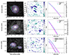 |
Fig. 1. Surface brightness profiles of the gas distribution of the galaxies BRI1335−0417, J081740 and the SGP38326 system, respectively from top to bottom. Left panels: surface brightness map of the [CII] emission. The emission is shown as contours in turquoise for the data and magenta for the model. The contour levels follow levels of emission of 4σ, 8σ and 16σ, where σ is the RMS noise in the total map. We show the beam of the observations in the bottom left. Middle panel: residual map normalised by the RMS noise according to the colourbar shown. We show the centre of the best-fit model of each galaxy with a small cross. Right panel: 1D profile of the average gas emission in concentric ellipses (turquoise) and the best-fit Sérsic model (magenta), the dotted line shows the 4σ level above the noise. In the bottom panel we show the galaxies SGP38326−1 and SGP38326−2 together, as they have to be fitted simultaneously, and we mask the emission of SGP38326−3 in the bottom left corner. |
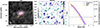 |
Fig. 2. Surface brightness profile of the dust distribution of the galaxy J081740, the other galaxies are shown in Fig. B.1. Left panel: surface brightness map of the dust continuum. The emission is shown as contours in orange for the data and in violet for the best-fit model. The contour levels follow levels of emission of 4σ, 8σ and 16σ, where σ is the RMS noise in the total map. We show the beam of the observations in the bottom left. Middle panel: residual map normalised by the RMS noise according to the colourbar shown. We show the centre of the best-fit model of the galaxy with a small cross. Right panel: 1D profile of the average gas emission in concentric ellipses (orange) and the best-fit Sérsic model (violet), the black dotted line shows the 4σ level above the noise. |
Gas and dust continuum surface brightness.
3.2. Mass decomposition of the rotation curves
Here, we present the fiducial dynamical models of the galaxies in our sample. Following the methods described in Sect. 2.6 we decompose the rotation curves of the galaxies into three mass components: stars, gas and a CDM halo. The procedure employed for the dynamical modelling of the galaxies J081740, SGP38326−1 and SGP38326−2 is the same: a single spherical Sérsic profile for the stars with free n, an exponential profile considering a razor-thin disc for the gas following the [CII] surface brightness and a spherical NFW CDM halo with the priors described in Table 2. However, for the galaxy BRI1335−0417, a different approach was taken, wherein the baryon fraction was fixed to the cosmological baryon fraction. This is due to the fact that the literature estimates for the gas mass of BRI1335−0417 are too high for its rotation curve. Therefore, as our fiducial model we assume a scenario that maximises the gas mass while still containing a marginally realistic CDM halo which provides an upper limit on the estimate of the total baryonic mass. We discuss this further in Appendix C.
In Fig. 3, we show the rotation curves derived from the [CII] kinematics. These rotation curves are corrected for pressure support following Eq. (3), so that we are plotting the circular speeds (further description of this is provided in Appendix A). Similarly to local galaxies, the shapes of the rotation curves of z ∼ 4 galaxies are diverse: BRI1335−0417 has a bump in the inner region that resembles the dynamical signature of a bulge; the rotation curves of J081470 and SGP38326−1 seem to flatten at large radii; and the rotation curve of SGP38326−2 has a shallow gradient. In Fig. 3, we overlap the contributions to the circular speeds by the stellar component, the gas disc and the CDM halo, as well as the total circular speed of our model (in black) that matches the observed rotation curve (in blue). In Table 4, we display the best-fit parameters that define the different components shown in Fig. 3. Additionally, in Appendix C we show the posterior distribution of the best-fit parameters and discuss some extra tests to probe the limitations of our data.
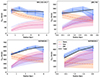 |
Fig. 3. Fiducial dynamical model for the galaxies. We show the measured circular speed, i.e. the rotation curve corrected for pressure support, as the blue shaded region. We also show the circular speed predicted by our model in black. The circular speed of the different mass components in the galaxies are shown as different shaded regions: stellar component (dash-dot line, orange), gas disc (dashed line, pink) and NFW CDM halo (dotted line, blue). In the case of BRI1335−0417, we fix the CDM halo to the cosmological baryon fraction. As explained in the main text, due to difficulties in breaking the degeneracy of the gas and DM contribution to the rotation curve we keep the CDM halo fixed to provide an upper limit on the baryon components. |
Results of the fiducial mass decomposition models.
We find that our rotation curve decomposition can constrain the stellar mass for the four galaxies reasonably well, placing our sample in a considerably massive regime, with stellar masses in between log(M*/M⊙) = 10.3 − 11.0. The accuracy of these estimates is due to the fact that the stellar component dominates the central region of the rotation curve, as a consequence, the inner shape of the rotation curve can only be reproduced by a massive stellar component. We find that this is only possible with stellar profiles with a high Sérsic index, indicating that a massive compact stellar distribution, such as a bulge, is present in all of the four galaxies. We note that the effective radius of such a component cannot be constrained with precision with the current data, although, we use physically motivated priors that provide plausible limits. Moreover, in spite of all the assumptions involved, we obtain effective radii for the stellar component compatible with values recently found with JWST observations of z > 2 galaxies (Ormerod et al. 2024; Tadaki et al. 2023).
The gas mass is constrained for J081740, SGP38326−1 and SGP38326−2, while for BRI1335−0417 we find an upper limit that is driven by the imposition of the cosmological baryon fraction. In general, the values of the gas masses have larger uncertainties than those for the stellar masses. This is because at small radii the stellar component is dominant, while at larger radii the main contribution to the rotation curve comes from both the gas and the CDM halo. Given the low concentration of DM at z ∼ 4 and that we are still only probing the relatively inner regions of these galaxies, the contribution of the CDM halo is hard to discern from the contribution of the gas. For example, considering a concentration of 3.4, an NFW halo with a virial mass of 1012 M⊙ produces a circular speed of about only 90 km s−1 lower than a halo with a virial mass of 1013 M⊙ at 3 kpc from the galactic centre. Combining this with the large uncertainties regarding the conversion between the CO luminosity and the gas mass then it becomes difficult to disentangle and constrain both the gas mass and the CDM halo mass with the current data. However, we can clearly see a pattern regarding the DM content of these galaxies in which they all prefer baryon dominated models as seen by the posterior distributions that has a maximum close to the lower edge of the prior (see Fig. C.1). Finally, we find that the gas mass of the galaxies range between log(Mgas/M⊙) = 9.8 − 11.3 and we find CDM halos masses ranging between log(M200/M⊙) = 11.2 − 13.3 with baryon fractions of 0.006 up to the cosmological baryon fraction of 0.187.
In Table 5, we report other relevant properties that can be derived by the direct results of the mass decomposition: we show the gas fractions, defined as fgas = Mgas/Mbar; the baryonic effective radius, defined as the radius that comprises half of the baryonic mass (Reff, bar); and the disc fraction, defined as the fraction of baryons to DM inside the baryonic effective radius (fdisc). Recently, Bland-Hawthorn et al. (2023) showed that these parameters can be used to predict the capability of a galaxy to form a stable bar. The four galaxies in our sample are above the thresholds set in Bland-Hawthorn et al. (2023), indicating that all of these discs have high enough baryon concentrations that could enable the quick formation of a stable bar. To further support this prediction, Tsukui et al. (2024) performed a thorough analysis of the [CII] and dust emissions in BRI1335−0417 suggesting the presence of a strong bar. Moreover, in general, our sample shows a diverse range of gas fractions, compatible to those found at z > 1 (Tacconi et al. 2020; Dessauges-Zavadsky et al. 2020; Aravena et al. 2016; Decarli et al. 2016).
Other properties derived from the results of the mass decomposition.
3.3. Star formation rates and stellar masses
In Fig. 4, we show the position of our galaxies in the SFR versus stellar mass plane, compared to the main sequence relation at z = 4.5 from Speagle et al. (2014). For our galaxies, we use the stellar masses derived from the mass decomposition of the rotation curves. The SFRs are derived from IR luminosities and converted to a Chabrier IMF as described in Sect. 2.2. We also show two thresholds for starburst galaxies: four times above the main sequence (Rodighiero et al. 2011) and the starburst bimodality (Rinaldi et al. 2022), which is an empirical division between main sequence and starburst galaxies at high-z in the specific SFRs first proposed by Caputi et al. (2017). We conclude that our sample is diverse in terms of SFR: J081740 is a main sequence galaxy, BRI1335−0417 and SGP38326−2 are both starburst and SGP38326−1 is borderline into the starburst region.
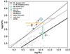 |
Fig. 4. Stellar mass vs. star formation rate. Our galaxies are represented by coloured circles according to the legend. We also show some other galaxies in the literature at similar redshift (Rizzo et al. 2020, 2021; Faisst et al. 2020; Lelli et al. 2021). The black line shows the main sequence relation at z = 4.5 from Speagle et al. (2014), while the dashed and dotted lines show the starburst/main sequence boundary according to Rodighiero et al. (2011) and Rinaldi et al. (2022), respectively. |
3.4. Origin of turbulence
As was pointed out in the introduction to this paper, the velocity dispersion measured in cold gas components, in particular CO and [CII], is mostly contributed by turbulence as thermal broadening can be considered negligible. An accurate estimation of the velocity dispersion allows us to investigate the potential drivers of turbulence within the ISM.
In high-z galaxies, gravitational instabilities and star formation feedback are believed to be the primary drivers of gas turbulence (Bournaud et al. 2007; Genzel et al. 2011; Krumholz & Burkhart 2016). These galaxies have higher gas fractions and densities compared to those in the local Universe (Tacconi et al. 2010, 2013; Decarli et al. 2016; Scoville et al. 2017). This abundance of gas not only promotes elevated star formation rates but can also cause more significant disruptions to the equilibrium of the gas disc (Tacconi et al. 2013). Here, we investigate which of these two possible scenarios are more likely: gas turbulence driven by gravitational instabilities in the disc and turbulence driven by stellar feedback.
3.4.1. Gravitational instabilities
To test the hypothesis that the gas turbulence in our sample is driven by gravitational instabilities, we compare the observed gas velocity dispersions to those expected by the analytical model from Krumholz et al. (2018). This model considers an axisymmetric disc of gas and stars in a DM halo, where the gas and stars have isotropic velocity dispersions and the disc is in both vertical hydrostatic and energy equilibrium. The model accounts for the energy contributed by star formation feedback and gravitational potential energy from inward gas flow. One main assumption of this model is that the gas in the disc self-regulates the inflow rate to maintain marginal stability.
We start by comparing our data to two models from Krumholz et al. (2018): the scenario with only gravitational instabilities as the driver of turbulence and the scenario with only stellar feedback shown in Fig. 5. Although in reality both scenarios could be present simultaneously, we choose to analyse these two cases individually to understand which one gets closer to reproduce the data. In both scenarios we use the fiducial parameters for high-z galaxies as reported in Krumholz et al. (2018) with different circular speeds that cover the range of velocities observed in our sample. On the left panel, we explore the σ–SFR relation for the gravity driven scenario assuming that the stellar feedback does not contribute to the turbulence. On the right panel, we explore the scenario of stellar feedback driven turbulence, in which there is no mass transport in the disc and the star formation efficiency is free to vary according to physical properties of the galaxy. Both assume that the Toomre Q parameter, which related to the local stability of the disc (Toomre 1964), is always equal to a marginally stable system.
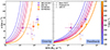 |
Fig. 5. Comparison of the observed gas velocity dispersion and star formation rate to expectations from analytical models from Krumholz et al. (2018). Left panel: different expectations from the model considering only gravitational instabilities as the driver of turbulence assuming fiducial parameters for high-z galaxies (solid lines). Right panel: different expectations from the model considering only stellar feedback as the driver of turbulence (solid lines). The models (solid lines) are colour-coded according to the maximum circular speed of the galaxies. We show our galaxies (Roman-Oliveira et al. 2023) and other resolved observations from the literature (Fraternali et al. 2021; Rizzo et al. 2021; Lelli et al. 2021) according to the legend. |
Figure 5 suggests that, for the typical range of SFR of z ∼ 4.5 galaxies, the analytical model including gravitational instabilities overestimates the level of turbulence in the gas discs. Instead, the stellar feedback only model is significantly better at reproducing the data trends, predicting velocity dispersions more similar to those observed. Moreover, despite the low-number statistics, we do not find any clear gradient in the rotation velocities of the observed dataset that follows the ones expected from either models, indicating that the turbulence might not be related to the total halo mass.
3.4.2. Stellar feedback
Following up on the evidence that the stellar feedback only models perform better than the gravity only models from Krumholz et al. (2018), we now compare our data with the simple model described in Sect. 2.7. Here we estimate the maximum possible energy that can be injected by SNII into the ISM of the galaxies given their current SFRs and compare to the turbulent energy present in the discs estimated from the observed velocity dispersions.
We show this comparison in Fig. 6, where the x-axis shows the maximum injectable energy expected from SNII calculated with Eq. (8) and assuming a supernova kinetic efficiency of 1. In the y-axis, we show the observed turbulent energy as calculated with Eq. (9) using the estimated total gas mass of each galaxy (see Table 4) and the observed velocity dispersion averaged across the radial extent of the disc as reported in Roman-Oliveira et al. (2023). Since we do not have reliable information about the thickness of gas discs, we analyse two different assumptions: one with a relatively thin disc (h = 0.3 kpc, thin ellipse) and a thick disc (h = 1.0 kpc, thick ellipse). Figure 6 also has identity lines that represent the SNII efficiency η that is usually expected to be of the order of 10%. We find that the three of the galaxies are consistent with η ≈ 0.1 while BRI1335−0417 is more consistent with a lower efficiency of η ≈ 0.001 − 0.01. These are realistic values and indicate that the level of turbulence in the galaxies can be easily explained by the current SFR present in their discs, without the need of other drivers of turbulence. We note here that we do not have a strong constrain in the gas mass of BRI1335−0417, since we had to keep the baryon fraction fixed to the cosmological fraction, effectively forcing the DM halo mass to its minimum realistic value.
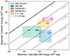 |
Fig. 6. Observed turbulent energy in the discs (Eq. (9)) vs. maximum possible energy that can be injected in the ISM from SNII (Eq. (8)). We explore the possibility of a thin (0.3 kpc, thin ellipse) and a thick disc (1 kpc, thick ellipse). BRI1335−0417 is shown as open marker due to the uncertainties on the dynamical estimate of the gas mass. |
4. Discussion
In this section, we discuss the main outcomes of the dynamical modelling of our sample, the origin of turbulence in the galaxies and a comparison of our sample with known scaling relations.
4.1. Compact and massive stellar component
One of the main outcomes of the dynamical models described in Sect. 3.2 is that the stellar component is described by a compact Sérsic profile with n ≳ 5. This indicates that a large portion of the stellar mass has to be concentrated in a compact region (< 2 kpc) in the centre of the galaxies. This could be a compact stellar disc or, more likely, a stellar bulge. This is in line with other recent works that report dynamical signatures of bulges in z > 4 galaxies (Rizzo et al. 2021; Lelli et al. 2021; Tripodi et al. 2023). In particular, Rizzo et al. (2021) reported steep rises in the rotation curve similar to those found in local galaxies with significant bulge components. In Lelli et al. (2021) and Tripodi et al. (2023), there is a significant increase in the rotation velocity in the innermost resolution element that can only be reproduced in the dynamical modelling by a massive bulge component. These are similar to the rotation curve of BRI1335−0417 shown in Fig. 3 which shows an increased velocity at the innermost radius compared to the outskirts. For BRI1335−0417 in particular, we also observe a high concentration of dust in the centre as the best-fit surface brightness profile suggests a Sérsic index of ∼4. This could be related to the presence of a concentrated star formation region and perhaps a bulge still in formation. It is also a possibility that the concentrated dust emission could be related to the fact that BRI1335−0417 is a QSO host; however, we attempt to fit the surface brightness of the dust emission with a Sérsic + PSF components and we find no evidence that it provides a better fit. As for the other galaxies in our sample, even though they do not show such a pronounced inner rise in the rotation curves, all of them require a stellar component with a Sérsic index higher than 4 to be able to reproduce the high inner circular speeds.
One may wonder whether the high rotation velocities that we observe in the inner regions could be explained by another component different from the stellar one. However, a CDM halo cannot explain velocities of such a magnitude considering that there is essentially no leverage in the concentration parameter at z ∼ 4 (Child et al. 2018; Correa et al. 2015; Dutton & Macciò 2014). Moreover, a central supermassive of 109 M⊙ can only give velocities of ∼200 km s−1 in the inner ∼100 pc, while we observe these velocities typically within the inner 2 kpc from the centre (see inner points of our rotation curves in Fig. 3). The only alternative possibility would be an accumulation of gas in a phase that is completely missed by the [CII] emission. This seems quite unlikely especially considering that [CII] is expected to trace all major phases of the cold ISM. Thus we conclude that the presence of very compact stellar components in our galaxies is very likely.
The above conclusion opens questions as to the which of the pathways of bulge formation can be so efficient in forming bulges so early. There are several processes that may form bulges, such as mergers or gravitational instabilities in the stellar discs (Kormendy & Kennicutt 2004; Kormendy & Ho 2013; Ishibashi & Fabian 2014). Another possibility is that bulges can be formed in discs with high fraction of baryonic mass with respect to the DM halo within the baryonic effective radius (fdisc in Table 5). In a recent work by Bland-Hawthorn et al. (2023), they predict that such high baryonic systems are very efficient at forming persistent bars, but also that in the presence of high gas fractions a bulge can be formed almost instantaneously in the centre of the galaxies. Independently on the specific mechanism, our findings suggest that the process of bulge formation has to happen rapidly and in the early phases of formation of massive galaxies (Ferreira et al. 2022; Jacobs et al. 2023; Kartaltepe et al. 2023). In fact, the bulges in galaxies at z ∼ 4.5 may indicate that these galaxies are the progenitors of massive quenched galaxies that host mature bulges at z = 2 − 4 (Valentino et al. 2023; Ito et al. 2024; Lustig et al. 2021; Tacchella et al. 2015). Moreover, the discs we observe could also be possible progenitors of red discs recently observed with JWST at z ∼ 2 − 3 (Huang et al. 2023; Fudamoto et al. 2022; Wu et al. 2023; Nelson et al. 2023).
4.2. Scaling relations
In this section, we investigate how our sample of high-z discs are situated in Tully–Fisher-like relations and in the stellar-to-halo mass relation (SHMR).
4.2.1. Tully–Fisher relations
In Fig. 7, we show the distribution of our sample with respect to the local BTFR (left panel) and the ETG analogue of the Tully–Fisher relation (right panel). The latter, as mentioned in the Introduction, is derived using the rotation velocities of the inner CO discs in local ETGs. We discuss both these panels separately below.
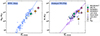 |
Fig. 7. Baryonic Tully–Fisher relation (left panel) and the analogue of the Tully–Fisher relation for ETGs (right panel). Left panel: Baryonic mass and the circular speed on the flat region of the rotation curves of local disc galaxies and the best-fit BTFR relation in blue (Lelli et al. 2016b). Right panel: stellar masses and inner rotation of local ETGs with stellar kinematics in purple (Lelli et al. 2017) and with inner CO rotating discs in violet (Davis et al. 2016). We show the baryonic mass and external circular speed of our sample according to the legend, in the right panel, we also show their stellar mass (stars). |
On the left panel of Fig. 7, we compare our sample to the BTFR for local disc galaxies where we show the disc galaxies from the Spitzer Photometry and Accurate Rotation Curves survey (SPARC, blue markers, Lelli et al. 2016a) and the BTFR best-fit relation from Lelli et al. (2016b). Here we show the baryonic masses of these galaxies and the circular speed estimated in the flat part of their rotation curves as obtained from kinematic models of the discs observed in HI. For our galaxies, we plot the total baryonic mass derived from the mass decomposition of the rotation curves and the external circular speeds defined as the average of the circular speed from the outer two resolution independent elements. We note that, like we do in the previous plots, we display BRI1335−0417 with an open symbol as we only have upper limits in the baryonic mass and therefore its placement in the BTFR is more uncertain. We find that, for the galaxies with a more reliable baryonic mass, there is a shift from the relation towards higher velocities for a fixed mass. This trend goes in the same direction as the cosmic evolution predicted by simulations and theoretical models (Posti et al. 2019; Torrey et al. 2014). However, we highlight that this is a small sample and that these galaxies are unlikely to be the progenitors of local disc galaxies. Therefore, it is difficult to draw firm conclusions and further comparison with theoretical models is needed.
On the right panel of Fig. 7, we compare our sample to local ETGs, both elliptical and lenticular galaxies, from the MASSIVE survey (violet markers, Ma et al. 2014). This subset of galaxies have small molecular gas discs extending out to 1−2 kpc that are buried within the stellar component of the host galaxy (Davis et al. 2013, 2011). We show the rotation derived from the velocity width of these small discs traced by the CO(J = 1 − 0) emission, revised by Davis et al. (2016) and Fraternali et al. (2021) for better estimates of their inclinations. The total stellar masses of the local galaxies are derived from a K-band luminosity assuming an M/L = 0.5 M⊙/L⊙, K. We highlight that, unlike the disc Tully–Fisher shown in the left panel, we show the stellar mass instead of the baryonic mass here. Moreover, we include a sample of ETGs from the ATLAS3D survey (Cappellari et al. 2011). This comprises lenticular, disc-like elliptical and boxy elliptical galaxies with available stellar kinematics, therefore also tracing mostly the inner parts of the galaxies (purple markers, Lelli et al. 2017). We also plot the best-fit relation from Davis et al. (2016), which has a shallower slope than the relation for discs shown on the left panel. We see that when we look at these inner rotations, which trace the baryon dominated inner potential of the galaxies, they deviate from the Tully–Fisher relation for disc galaxies from Lelli et al. (2016b) as, in particular at high masses, they move towards a region of fast rotation with respect to their luminous mass content, as also noted by Davis et al. (2016). For our galaxies, we position them according to both their stellar mass (coloured stars in the panel) and their baryonic mass (stars + gas, squares) with the same external circular speed as shown in the left panel. We see that our z ∼ 4.5 galaxies tend to be shifted from the local ETG relation when comparing their stellar masses, but this shift disappears once we assume that their gas content will be fully converted into stars by z = 0, similar to what was observed in Fraternali et al. (2021). This suggests that, these z ∼ 4.5 galaxies are largely formed in the inner regions as they have gravitational potentials similar to local ETGs and do not need to accrete more gas in order to be consistent with the local relation. Given that it is rare to find spiral galaxies rotating at or above ∼300 km s−1 (Di Teodoro et al. 2023; Ogle et al. 2019; Posti et al. 2018), we can expect that as the gas is converted into stars, the galaxies should undergo morphological changes and become more pressure supported (potentially through a series of minor or major mergers, see Hilz et al. 2013; Naab & Ostriker 2009; Naab et al. 2009). Overall these findings give dynamical support to the scenario in which these massive z ∼ 4.5 galaxies are likely progenitors of local ETGs (Fraternali et al. 2021; Rizzo et al. 2020; Toft et al. 2014; Barro et al. 2014).
4.2.2. The stellar-to-halo mass relation
The SHMR is crucial in understanding the relationship between baryonic matter and the DM halos of galaxies as it traces the efficiency of the conversion of baryons into stars as a function of the halo mass, providing a proxy of the efficiency of galaxy formation over cosmic time (Moster et al. 2010; Behroozi et al. 2013). Unlike the BTFR, the SHMR has been extended up to z ∼ 6 with the use of abundance-matching techniques. However, to date, the SMHR has been estimated only up to z ∼ 1 with direct dynamical estimates of CDM halo masses of individual galaxies (Bouché et al. 2022). Recent studies suggest that the SHMR may be dependent on the morphology of galaxies, where the relation breaks at the massive end with massive discs containing higher stellar mass fractions than elliptical galaxies (Correa & Schaye 2020; Marasco et al. 2020; Rodriguez-Gomez et al. 2022). Moreover, this was supported by Posti et al. (2019) and Di Teodoro et al. (2023) that showed empirically that local massive disc galaxies deviate from the relation obtained from abundance-matching techniques. It was suggested that these massive discs must have evolved at near isolation, without going through disruptive events such as AGN feedback or major mergers.
In Fig. 8, we present the SHMR in the form of the stellar-to-halo mass fraction (M*/Mh) as a function of the halo mass (Mh). We compare this to the expected relation from abundance-matching techniques at 4.5 < z < 5.5 from Shuntov et al. (2022). We see that the curve is reasonably compatible with the data, with the exception of BRI1335−0417, which has only a lower limits on the CDM halo mass. We note that, at least for this sample of z ∼ 4.5 massive disc galaxies, we do not find any significant deviation towards higher stellar fractions at the massive end.
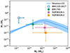 |
Fig. 8. Stellar-to-halo mass relation. We show the stellar-to-halo mass fraction on the y-axis versus the halo mass in the x axis. Our galaxies are shown as coloured circle markers according to the legend and the expected SHMR relation for central halos at 4.5 < z < 5.5 as a curve with 16th, 50th and 84th percentiles from Shuntov et al. (2022). |
5. Conclusions
In this paper, we provide mass decomposition of the rotation curves of four galaxies at z ∼ 4.5 using resolved kinematics traced by the [CII] 158 μm emission line observed with ALMA. We used this decomposition to determine the main properties of the various matter components in galaxies of the Early Universe. We also investigated the possible origin of turbulence in the cold gas component of these galaxies to gain insights into the main contributions to the observed velocity dispersions. Our main results can be summarised as follows:
-
From the rotation curve decomposition, we constrain the stellar masses (ranging between log(M*/M⊙) = 10.3 and 11.0) and gas masses (ranging between log(Mgas/M⊙) = 9.8 and 11.3). We also estimate the DM halo mass of the galaxies (ranging between log(M200/M⊙) = 11.2 − 13.3), albeit with larger uncertainties. We find that our galaxies are strongly baryon dominated in the regions probed (inner 3 to 5 kpc) and that they have a variety of gas-to-baryon fractions, from 0.16 to 0.87.
-
We investigated the origin of the turbulence in the gas discs by comparing the observed [CII] velocity dispersion to analytical models of turbulence driven by either gravitational instabilities or stellar feedback. We find that the observed gas turbulence in the discs can be fully reproduced by the stellar feedback alone, without the need for large-scale gravitational instabilities or other mechanisms. We conclude that the observed gas turbulence can be easily maintained by supernova explosions with efficiencies of only 10% or less.
-
Our rotation curve decompositions indicate that there must be a massive compact stellar component dominating within the inner 2 kpc of the galaxies in our sample and compatible with what would be expected from a stellar bulge. This dynamical evidence, already suggested by other similar studies of galaxies at z = 4 − 5, can be validated by upcoming JWST/NIRCam observations of the stellar continuum of these galaxies.
-
With the properties derived from the rotation curve decomposition, we place the galaxies in our sample into two scaling relations: the stellar-to-halo mass relation, where our data are in broad agreement with the relation obtained from abundance-matching techniques; and two versions of the Tully–Fisher relation. Compared to the local baryonic Tully–Fisher relations, our galaxies show a shift towards higher rotation velocities, as expected from theory. Instead, in the ETG analogue of the Tully–Fisher relation, our galaxies overlap with local ETGs once their gas mass is added to the stellar mass, suggesting that, at least in the inner regions, they have gathered the majority of their baryonic mass already at z ∼ 4.5.
Finally, we reiterate that the spatially resolved kinematics of galaxies can be used as a powerful tool for studying the physical mechanisms involved in galaxy formation and evolution. It is crucial to obtain constraints on the internal structure and morphology of galaxies, which can provide insights into the complex interactions between DM, gas, stars, and feedback processes in the ISM. We emphasise that the detailed analysis carried out in this paper, in particular the mass decomposition of the rotation curves, requires at least six independent resolution elements along the major axis in any single galaxy. ALMA is currently the only instrument that can provide sufficient S/R and angular resolution to achieve these requirements. Such observations are heavily time consuming but critical, and in the future we should push for even higher data quality to be able to investigate the shape of the DM halos. We can achieve this quality with JWST, which will give us spatially resolved information for the stellar component. We can combine this with higher sensitivity ALMA data to probe the outer regions of the rotation curve that are more DM dominated.
Acknowledgments
We thank Vasily Kokorev and Takafumi Tsukui for the discussion on the SFR of BRI1335-0417, Marko Shuntov for the SHMR and Joss Bland-Hawthorn for the discussion on the disc fraction and the formation of bars. F.R.O. and F.F. acknowledge support from The Dutch Research Council (NWO) through the Klein-1 Grant code OCEN2.KLEIN.088. F.R. acknowledges support from the European Union’s Horizon 2020 research and innovation program under the Marie Sklodowska-Curie grant agreement No. 847523 “INTERACTIONS” and the Cosmic Dawn Center which is funded by the Danish National Research Foundation under grant No. 140. The project leading to this publication has received support from ORP, that is funded by the European Union’s Horizon 2020 research and innovation programme under grant agreement No. 101004719 [ORP]. We acknowledge extensive assistance from Allegro, the European ALMA Regional Center node in the Netherlands. The Joint ALMA Observatory is operated by ESO, AUI/NRAO and NAOJ. This work makes use of the following ALMA data: ADS/JAO.ALMA#2015.1.00330.S, ADS/JAO.ALMA#2017.1.00127.S, #2017.1.00394.S, #2017.1.01052.S, #2018.1.00001.S. ALMA is a partnership of ESO (representing its member states), NSF (USA) and NINS (Japan), together with NRC (Canada), MOST and ASIAA (Taiwan), and KASI (Republic of Korea), in cooperation with the Republic of Chile. This publication makes use of data products from the Wide-field Infrared Survey Explorer, which is a joint project of the University of California, Los Angeles, and the Jet Propulsion Laboratory/California Institute of Technology, funded by the National Aeronautics and Space Administration. Data Availability: The data underlying this article are public and available in the ALMA Science Archive, at https://almascience.nrao.edu/asax/. The processed data (i.e. the rotation curves corrected for ADC and the 0th-moment maps for the dust continuum and [CII] emission) along with the scripts to produce the figures in this paper are made available at Zenodo (DOI: https://doi.org/10.5281/zenodo.10707348).
References
- Aravena, M., Spilker, J. S., Bethermin, M., et al. 2016, MNRAS, 457, 4406 [Google Scholar]
- Astropy Collaboration (Robitaille, T. P., et al.) 2013, A&A, 558, A33 [NASA ADS] [CrossRef] [EDP Sciences] [Google Scholar]
- Astropy Collaboration (Price-Whelan, A. M., et al.) 2018, AJ, 156, 123 [Google Scholar]
- Astropy Collaboration (Price-Whelan, A. M., et al.) 2022, ApJ, 935, 167 [NASA ADS] [CrossRef] [Google Scholar]
- Bacchini, C., Fraternali, F., Iorio, G., et al. 2020, A&A, 641, A70 [NASA ADS] [CrossRef] [EDP Sciences] [Google Scholar]
- Barro, G., Faber, S. M., Pérez-González, P. G., et al. 2014, ApJ, 791, 52 [Google Scholar]
- Behroozi, P. S., Wechsler, R. H., & Conroy, C. 2013, ApJ, 762, L31 [NASA ADS] [CrossRef] [Google Scholar]
- Binney, J., & Tremaine, S. 2008, Galactic Dynamics: Second Edition (Princeton: Princeton University Press) [Google Scholar]
- Bland-Hawthorn, J., Tepper-Garcia, T., Agertz, O., & Freeman, K. 2023, ApJ, 947, 80 [NASA ADS] [CrossRef] [Google Scholar]
- Bolatto, A. D., Wolfire, M., & Leroy, A. K. 2013, ARA&A, 51, 207 [CrossRef] [Google Scholar]
- Boogaard, L. A., van der Werf, P., Weiss, A., et al. 2020, ApJ, 902, 109 [NASA ADS] [CrossRef] [Google Scholar]
- Bouché, N. F., Bera, S., Krajnović, D., et al. 2022, A&A, 658, A76 [NASA ADS] [CrossRef] [EDP Sciences] [Google Scholar]
- Bournaud, F., Elmegreen, B. G., & Elmegreen, D. M. 2007, ApJ, 670, 237 [Google Scholar]
- Cappellari, M., Emsellem, E., Krajnović, D., et al. 2011, MNRAS, 413, 813 [Google Scholar]
- Caputi, K. I., Deshmukh, S., Ashby, M. L. N., et al. 2017, ApJ, 849, 45 [Google Scholar]
- Carilli, C. L., & Walter, F. 2013, ARA&A, 51, 105 [NASA ADS] [CrossRef] [Google Scholar]
- Casey, C. M., Narayanan, D., & Cooray, A. 2014, Phys. Rep., 541, 45 [Google Scholar]
- Chabrier, G. 2003, PASP, 115, 763 [Google Scholar]
- Child, H. L., Habib, S., Heitmann, K., et al. 2018, ApJ, 859, 55 [NASA ADS] [CrossRef] [Google Scholar]
- Cimatti, A., Fraternali, F., & Nipoti, C. 2019, Introduction to Galaxy Formation and Evolution: From Primordial Gas to Present-Day Galaxies (Cambridge: Cambridge University Press) [Google Scholar]
- Cochrane, R. K., Hayward, C. C., Anglés-Alcázar, D., et al. 2019, MNRAS, 488, 1779 [NASA ADS] [CrossRef] [Google Scholar]
- Colina, L., Crespo Gómez, A., Álvarez-Márquez, J., et al. 2023, A&A, 673, L6 [NASA ADS] [CrossRef] [EDP Sciences] [Google Scholar]
- Correa, C. A., & Schaye, J. 2020, MNRAS, 499, 3578 [Google Scholar]
- Correa, C. A., Wyithe, J. S. B., Schaye, J., & Duffy, A. R. 2015, MNRAS, 452, 1217 [CrossRef] [Google Scholar]
- Costantin, L., Pérez-González, P. G., Guo, Y., et al. 2023, Nature, 623, 499 [NASA ADS] [CrossRef] [Google Scholar]
- da Cunha, E., Groves, B., Walter, F., et al. 2013, ApJ, 766, 13 [Google Scholar]
- Davis, T. A., Bureau, M., Young, L. M., et al. 2011, MNRAS, 414, 968 [Google Scholar]
- Davis, T. A., Alatalo, K., Bureau, M., et al. 2013, MNRAS, 429, 534 [Google Scholar]
- Davis, T. A., Greene, J., Ma, C.-P., et al. 2016, MNRAS, 455, 214 [Google Scholar]
- Decarli, R., Walter, F., Aravena, M., et al. 2016, ApJ, 833, 69 [Google Scholar]
- Dessauges-Zavadsky, M., Ginolfi, M., Pozzi, F., et al. 2020, A&A, 643, A5 [NASA ADS] [CrossRef] [EDP Sciences] [Google Scholar]
- Di Teodoro, E. M., & Fraternali, F. 2015, MNRAS, 451, 3021 [Google Scholar]
- Di Teodoro, E. M., Fraternali, F., & Miller, S. H. 2016, A&A, 594, A77 [NASA ADS] [CrossRef] [EDP Sciences] [Google Scholar]
- Di Teodoro, E. M., Posti, L., Fall, S. M., et al. 2023, MNRAS, 518, 6340 [Google Scholar]
- Dunne, L., Maddox, S. J., Papadopoulos, P. P., Ivison, R. J., & Gomez, H. L. 2022, MNRAS, 517, 962 [NASA ADS] [CrossRef] [Google Scholar]
- Dutton, A. A., & Macciò, A. V. 2014, MNRAS, 441, 3359 [Google Scholar]
- Ejdetjärn, T., Agertz, O., Östlin, G., Renaud, F., & Romeo, A. B. 2022, MNRAS, 514, 480 [CrossRef] [Google Scholar]
- Faisst, A. L., Schaerer, D., Lemaux, B. C., et al. 2020, ApJS, 247, 61 [NASA ADS] [CrossRef] [Google Scholar]
- Ferreira, L., Adams, N., Conselice, C. J., et al. 2022, ApJ, 938, L2 [NASA ADS] [CrossRef] [Google Scholar]
- Ferreira, L., Conselice, C. J., Sazonova, E., et al. 2023, ApJ, 955, 94 [NASA ADS] [CrossRef] [Google Scholar]
- Fierlinger, K. M., Burkert, A., Ntormousi, E., et al. 2016, MNRAS, 456, 710 [NASA ADS] [CrossRef] [Google Scholar]
- Fraternali, F., Karim, A., Magnelli, B., et al. 2021, A&A, 647, A194 [NASA ADS] [CrossRef] [EDP Sciences] [Google Scholar]
- Fudamoto, Y., Ivison, R. J., Oteo, I., et al. 2017, MNRAS, 472, 2028 [NASA ADS] [CrossRef] [Google Scholar]
- Fudamoto, Y., Inoue, A. K., & Sugahara, Y. 2022, ApJ, 938, L24 [NASA ADS] [CrossRef] [Google Scholar]
- Genzel, R., Newman, S., Jones, T., et al. 2011, ApJ, 733, 101 [Google Scholar]
- Gillman, S., Gullberg, B., Brammer, G., et al. 2023, A&A, 676, A26 [NASA ADS] [CrossRef] [EDP Sciences] [Google Scholar]
- Gong, M., Ostriker, E. C., Kim, C.-G., & Kim, J.-G. 2020, ApJ, 903, 142 [CrossRef] [Google Scholar]
- Governato, F., Willman, B., Mayer, L., et al. 2007, MNRAS, 374, 1479 [NASA ADS] [CrossRef] [Google Scholar]
- Graham, A. W., & Driver, S. P. 2005, PASA, 22, 118 [NASA ADS] [CrossRef] [Google Scholar]
- Harrison, C. M., Johnson, H. L., Swinbank, A. M., et al. 2017, MNRAS, 467, 1965 [Google Scholar]
- Hilz, M., Naab, T., & Ostriker, J. P. 2013, MNRAS, 429, 2924 [NASA ADS] [CrossRef] [Google Scholar]
- Hodge, J. A., Carilli, C. L., Walter, F., et al. 2012, ApJ, 760, 11 [Google Scholar]
- Hopkins, P. F., Kereš, D., Oñorbe, J., et al. 2014, MNRAS, 445, 581 [NASA ADS] [CrossRef] [Google Scholar]
- Huang, S., Kawabe, R., Kohno, K., et al. 2023, ApJ, 958, L26 [NASA ADS] [CrossRef] [Google Scholar]
- Iorio, G., Fraternali, F., Nipoti, C., et al. 2017, MNRAS, 466, 4159 [NASA ADS] [Google Scholar]
- Ishibashi, W., & Fabian, A. C. 2014, MNRAS, 441, 1474 [NASA ADS] [CrossRef] [Google Scholar]
- Ito, k., Valentino, F., Brammer, G., et al. 2024, ApJ, 964, 192 [CrossRef] [Google Scholar]
- Jacobs, C., Glazebrook, K., Calabrò, A., et al. 2023, ApJ, 948, L13 [NASA ADS] [CrossRef] [Google Scholar]
- Jones, G. C., Carilli, C. L., Momjian, E., et al. 2016, ApJ, 830, 63 [NASA ADS] [CrossRef] [Google Scholar]
- Jones, G. C., Vergani, D., Romano, M., et al. 2021, MNRAS, 507, 3540 [NASA ADS] [CrossRef] [Google Scholar]
- Kaasinen, M., Walter, F., Novak, M., et al. 2020, ApJ, 899, 37 [NASA ADS] [CrossRef] [Google Scholar]
- Kamenetzky, J., Rangwala, N., Glenn, J., Maloney, P. R., & Conley, A. 2016, ApJ, 829, 93 [Google Scholar]
- Kartaltepe, J. S., Rose, C., Vanderhoof, B. N., et al. 2023, ApJ, 946, L15 [NASA ADS] [CrossRef] [Google Scholar]
- Kohandel, M., Pallottini, A., Ferrara, A., et al. 2020, MNRAS, 499, 1250 [Google Scholar]
- Koposov, S., Speagle, J., Barbary, K., et al. 2022, https://doi.org/10.5281/zenodo.6609296 [Google Scholar]
- Kormendy, J., & Ho, L. C. 2013, ARA&A, 51, 511 [Google Scholar]
- Kormendy, J., & Kennicutt, R. C. 2004, ARA&A, 42, 603 [Google Scholar]
- Kretschmer, M., Dekel, A., & Teyssier, R. 2022, MNRAS, 510, 3266 [NASA ADS] [CrossRef] [Google Scholar]
- Krumholz, M. R., & Burkhart, B. 2016, MNRAS, 458, 1671 [NASA ADS] [CrossRef] [Google Scholar]
- Krumholz, M. R., Burkhart, B., Forbes, J. C., & Crocker, R. M. 2018, MNRAS, 477, 2716 [CrossRef] [Google Scholar]
- Lagache, G., Cousin, M., & Chatzikos, M. 2018, A&A, 609, A130 [NASA ADS] [CrossRef] [EDP Sciences] [Google Scholar]
- Le Conte, Z. A., Gadotti, D. A., Ferreira, L., et al. 2024, MNRAS, 530, 1984 [NASA ADS] [CrossRef] [Google Scholar]
- Lelli, F., McGaugh, S. S., & Schombert, J. M. 2016a, AJ, 152, 157 [Google Scholar]
- Lelli, F., McGaugh, S. S., & Schombert, J. M. 2016b, ApJ, 816, L14 [Google Scholar]
- Lelli, F., McGaugh, S. S., Schombert, J. M., & Pawlowski, M. S. 2017, ApJ, 836, 152 [Google Scholar]
- Lelli, F., Di Teodoro, E. M., Fraternali, F., et al. 2021, Science, 371, 713 [Google Scholar]
- Lu, N., Cao, T., Díaz-Santos, T., et al. 2018, ApJ, 864, 38 [NASA ADS] [CrossRef] [Google Scholar]
- Lustig, P., Strazzullo, V., D’Eugenio, C., et al. 2021, MNRAS, 501, 2659 [NASA ADS] [CrossRef] [Google Scholar]
- Ma, C.-P., Greene, J. E., McConnell, N., et al. 2014, ApJ, 795, 158 [Google Scholar]
- Mac Low, M.-M. 1999, ApJ, 524, 169 [Google Scholar]
- Marasco, A., Fraternali, F., Heald, G., et al. 2019, A&A, 631, A50 [NASA ADS] [CrossRef] [EDP Sciences] [Google Scholar]
- Marasco, A., Posti, L., Oman, K., et al. 2020, A&A, 640, A70 [EDP Sciences] [Google Scholar]
- McGaugh, S. S. 2004, ApJ, 609, 652 [NASA ADS] [CrossRef] [Google Scholar]
- McGaugh, S. S., & Schombert, J. M. 2015, ApJ, 802, 18 [NASA ADS] [CrossRef] [Google Scholar]
- McGaugh, S. S., Schombert, J. M., Bothun, G. D., & de Blok, W. J. G. 2000, ApJ, 533, L99 [Google Scholar]
- McMullin, J. P., Waters, B., Schiebel, D., Young, W., & Golap, K. 2007, in Astronomical Data Analysis Software and Systems XVI, eds. R. A. Shaw, F. Hill, & D. J. Bell, AIP Conf. Ser., 376, 127 [Google Scholar]
- Mo, H., van den Bosch, F. C., & White, S. 2010, Galaxy Formation and Evolution (Cambridge: Cambridge University Press) [Google Scholar]
- Moster, B. P., Somerville, R. S., Maulbetsch, C., et al. 2010, ApJ, 710, 903 [Google Scholar]
- Naab, T., & Ostriker, J. P. 2009, ApJ, 690, 1452 [NASA ADS] [CrossRef] [Google Scholar]
- Naab, T., Johansson, P. H., & Ostriker, J. P. 2009, ApJ, 699, L178 [Google Scholar]
- Narayanan, D., Krumholz, M., Ostriker, E. C., & Hernquist, L. 2011, MNRAS, 418, 664 [NASA ADS] [CrossRef] [Google Scholar]
- Navarro, J. F., Frenk, C. S., & White, S. D. M. 1997, ApJ, 490, 493 [Google Scholar]
- Neeleman, M., Kanekar, N., Prochaska, J. X., Rafelski, M. A., & Carilli, C. L. 2019, ApJ, 870, L19 [NASA ADS] [CrossRef] [Google Scholar]
- Neeleman, M., Prochaska, J. X., Kanekar, N., & Rafelski, M. 2020, Nature, 581, 269 [Google Scholar]
- Neeleman, M., Walter, F., Decarli, R., et al. 2023, ApJ, 958, 132 [NASA ADS] [CrossRef] [Google Scholar]
- Nelson, D., Pillepich, A., Springel, V., et al. 2019, MNRAS, 490, 3234 [Google Scholar]
- Nelson, E. J., Suess, K. A., Bezanson, R., et al. 2023, ApJ, 948, L18 [NASA ADS] [CrossRef] [Google Scholar]
- Ogle, P. M., Lanz, L., Appleton, P. N., Helou, G., & Mazzarella, J. 2019, ApJS, 243, 14 [Google Scholar]
- Ohlin, L., Renaud, F., & Agertz, O. 2019, MNRAS, 485, 3887 [Google Scholar]
- Ormerod, K., Conselice, C. J., Adams, N. J., et al. 2024, MNRAS, 527, 6110 [Google Scholar]
- Orr, M. E., Hayward, C. C., Medling, A. M., et al. 2020, MNRAS, 496, 1620 [NASA ADS] [CrossRef] [Google Scholar]
- Oteo, I., Ivison, R. J., Dunne, L., et al. 2016, ApJ, 827, 34 [Google Scholar]
- Papadopoulos, P. P., Bisbas, T. G., & Zhang, Z.-Y. 2018, MNRAS, 478, 1716 [NASA ADS] [CrossRef] [Google Scholar]
- Planck Collaboration I. 2020, A&A, 641, A1 [NASA ADS] [CrossRef] [EDP Sciences] [Google Scholar]
- Popping, G., Pillepich, A., Calistro Rivera, G., et al. 2022, MNRAS, 510, 3321 [CrossRef] [Google Scholar]
- Posti, L., Fraternali, F., Di Teodoro, E. M., & Pezzulli, G. 2018, A&A, 612, L6 [NASA ADS] [CrossRef] [EDP Sciences] [Google Scholar]
- Posti, L., Marasco, A., Fraternali, F., & Famaey, B. 2019, A&A, 629, A59 [NASA ADS] [CrossRef] [EDP Sciences] [Google Scholar]
- Renaud, F., Bournaud, F., Kraljic, K., & Duc, P. A. 2014, MNRAS, 442, L33 [NASA ADS] [CrossRef] [Google Scholar]
- Rinaldi, P., Caputi, K. I., van Mierlo, S. E., et al. 2022, ApJ, 930, 128 [NASA ADS] [CrossRef] [Google Scholar]
- Rizzo, F., Vegetti, S., Powell, D., et al. 2020, Nature, 584, 201 [Google Scholar]
- Rizzo, F., Vegetti, S., Fraternali, F., Stacey, H. R., & Powell, D. 2021, MNRAS, 507, 3952 [NASA ADS] [CrossRef] [Google Scholar]
- Rizzo, F., Kohandel, M., Pallottini, A., et al. 2022, A&A, 667, A5 [NASA ADS] [CrossRef] [EDP Sciences] [Google Scholar]
- Robertson, B. E., Tacchella, S., Johnson, B. D., et al. 2023, ApJ, 942, L42 [NASA ADS] [CrossRef] [Google Scholar]
- Rodighiero, G., Daddi, E., Baronchelli, I., et al. 2011, ApJ, 739, L40 [Google Scholar]
- Rodney, S. A., Riess, A. G., Strolger, L.-G., et al. 2014, AJ, 148, 13 [Google Scholar]
- Rodriguez-Gomez, V., Genel, S., Fall, S. M., et al. 2022, MNRAS, 512, 5978 [NASA ADS] [CrossRef] [Google Scholar]
- Roman-Oliveira, F., Fraternali, F., & Rizzo, F. 2023, MNRAS, 521, 1045 [NASA ADS] [CrossRef] [Google Scholar]
- Rubin, V. C., Ford, W. K., & Thonnard, N. 1980, ApJ, 238, 471 [NASA ADS] [CrossRef] [Google Scholar]
- Schaye, J., Crain, R. A., Bower, R. G., et al. 2015, MNRAS, 446, 521 [Google Scholar]
- Scoville, N., Lee, N., Vanden Bout, P., et al. 2017, ApJ, 837, 150 [Google Scholar]
- Sersic, J. L. 1968, Atlas de Galaxias Australes (Cordoba, Argentina: Observatorio Astronomico) [Google Scholar]
- Shao, Y., Wang, R., Weiss, A., et al. 2022, A&A, 668, A121 [NASA ADS] [CrossRef] [EDP Sciences] [Google Scholar]
- Shuntov, M., McCracken, H. J., Gavazzi, R., et al. 2022, A&A, 664, A61 [NASA ADS] [CrossRef] [EDP Sciences] [Google Scholar]
- Skilling, J. 2004, in Bayesian Inference and Maximum Entropy Methods in Science and Engineering: 24th International Workshop on Bayesian Inference and Maximum Entropy Methods in Science and Engineering, eds. R. Fischer, R. Preuss, & U. V. Toussaint, AIP Conf. Ser., 735, 395 [NASA ADS] [CrossRef] [Google Scholar]
- Skilling, J. 2006, Bayesian Anal., 1, 833 [Google Scholar]
- Smit, R., Bouwens, R. J., Carniani, S., et al. 2018, Nature, 553, 178 [Google Scholar]
- Speagle, J. S. 2020, MNRAS, 493, 3132 [Google Scholar]
- Speagle, J. S., Steinhardt, C. L., Capak, P. L., & Silverman, J. D. 2014, ApJS, 214, 15 [Google Scholar]
- Tacchella, S., Carollo, C. M., Renzini, A., et al. 2015, Science, 348, 314 [NASA ADS] [CrossRef] [Google Scholar]
- Tacchella, S., Dekel, A., Carollo, C. M., et al. 2016, MNRAS, 457, 2790 [Google Scholar]
- Tacconi, L. J., Genzel, R., Neri, R., et al. 2010, Nature, 463, 781 [Google Scholar]
- Tacconi, L. J., Neri, R., Genzel, R., et al. 2013, ApJ, 768, 74 [NASA ADS] [CrossRef] [Google Scholar]
- Tacconi, L. J., Genzel, R., & Sternberg, A. 2020, ARA&A, 58, 157 [NASA ADS] [CrossRef] [Google Scholar]
- Tadaki, K.-I., Belli, S., Burkert, A., et al. 2020, ApJ, 901, 74 [NASA ADS] [CrossRef] [Google Scholar]
- Tadaki, K.-I., Kodama, T., Koyama, Y., et al. 2023, ApJ, 957, L15 [NASA ADS] [CrossRef] [Google Scholar]
- Tamburro, D., Rix, H. W., Leroy, A. K., et al. 2009, AJ, 137, 4424 [Google Scholar]
- Terzić, B., & Graham, A. W. 2005, MNRAS, 362, 197 [CrossRef] [Google Scholar]
- Tiley, A. L., Stott, J. P., Swinbank, A. M., et al. 2016, MNRAS, 460, 103 [Google Scholar]
- Toft, S., Smolčić, V., Magnelli, B., et al. 2014, ApJ, 782, 68 [Google Scholar]
- Toomre, A. 1964, ApJ, 139, 1217 [Google Scholar]
- Torrey, P., Vogelsberger, M., Genel, S., et al. 2014, MNRAS, 438, 1985 [CrossRef] [Google Scholar]
- Tripodi, R., Lelli, F., Feruglio, C., et al. 2023, A&A, 671, A44 [NASA ADS] [CrossRef] [EDP Sciences] [Google Scholar]
- Tsukui, T., & Iguchi, S. 2021, Science, 372, 1201 [NASA ADS] [CrossRef] [Google Scholar]
- Tsukui, T., Wisnioski, E., Krumholz, M. R., & Battisti, A. 2023, MNRAS, 523, 4654 [NASA ADS] [CrossRef] [Google Scholar]
- Tsukui, T., Wisnioski, E., Bland-Hawthorn, J., et al. 2024, MNRAS, 527, 8941 [Google Scholar]
- Tully, R. B., & Fisher, J. R. 1977, A&A, 54, 661 [NASA ADS] [Google Scholar]
- Übler, H., Förster Schreiber, N. M., Genzel, R., et al. 2017, ApJ, 842, 121 [Google Scholar]
- Valentino, F., Brammer, G., Gould, K. M. L., et al. 2023, ApJ, 947, 20 [NASA ADS] [CrossRef] [Google Scholar]
- van Albada, T. S., Bahcall, J. N., Begeman, K., & Sancisi, R. 1985, ApJ, 295, 305 [Google Scholar]
- Vogelsberger, M., Marinacci, F., Torrey, P., & Puchwein, E. 2020, Nat. Rev. Phys., 2, 42 [Google Scholar]
- Wagg, J., Carilli, C. L., Aravena, M., et al. 2014, ApJ, 783, 71 [NASA ADS] [CrossRef] [Google Scholar]
- Wu, Y., Cai, Z., Sun, F., et al. 2023, ApJ, 942, L1 [CrossRef] [Google Scholar]
- Yang, C., Omont, A., Beelen, A., et al. 2017, A&A, 608, A144 [NASA ADS] [CrossRef] [EDP Sciences] [Google Scholar]
- Yu, X., Bian, F., Krumholz, M. R., et al. 2021, MNRAS, 505, 5075 [NASA ADS] [CrossRef] [Google Scholar]
Appendix A: Asymmetric drift correction
As discussed in Section 2.6, to obtain the circular speed from the rotation velocity it is first necessary to correct the rotation curve for the gas pressure support by applying the asymmetric drift correction. Although 3DBAROLO can apply this correction during the kinematic fitting, it does so without convolving the [CII] surface brightness with the beam. To properly account for the spatial resolution, we assume that the gas is distributed as an exponential disc and use the best-fit disc scale length reported in Table 3. Therefore, we can rewrite the asymmetric drift correction from Equation 3 as
![Mathematical equation: $$ \begin{aligned} V_{\mathrm{A} }^2 = - R \sigma ^2 \frac{\partial }{\partial R} \left[\ln {(\sigma ^2 \exp {(-R/R_{\mathrm{gas} }}}))\right], \end{aligned} $$](/articles/aa/full_html/2024/07/aa48828-23/aa48828-23-eq49.gif) (A.1)
(A.1)
and consequently,
 (A.2)
(A.2)
To apply this correction to the rotation velocity, we numerically calculate the slope of lnσ at each radial element. In Figure A.1 we show the result of the asymmetric drift correction for BRI1335-0417, which, in spite of the difference in methodology, agrees with the circular speed derived with 3DBAROLO.
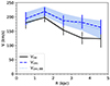 |
Fig. A.1. Comparison between the original rotation velocity obtained from the kinematic modelling (Vrot) and the circular speed after the asymmetric drift correction was applied with the method described in this Appendix (Vcirc) and the one obtained with 3DBAROLO (Vcirc, BB). |
Appendix B: Surface brightness models best-fit posteriors
Here we show the posterior distributions of the best-fit surface brightness models for the gas and dust emission obtained as described in Section 2.3. We fit the surface brightness at the effective radius (Ie), the effective radius (Reff), the centre (x0, y0), ellipticity (ϵ) and position angle (PA). For the dust emission of BRI1335-0417 we let the Sérsic index (n) free to vary as it is significantly different from 1.
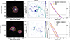 |
Fig. B.1. Surface brightness profiles of the dust distribution. Details are as described in the caption of Figure 1. |
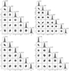 |
Fig. B.2. Posterior distributions of the surface brightness fits of the gas and dust distribution of the galaxies. Top left panel: [CII] emission of BRI1335-0417. Top right panel: Dust continuum emission of BRI1335-0417. Bottom left panel: [CII] emission of J081740. Bottom right panel: Dust continuum emission of J081740. All fits displayed have the Sérsic index fixed to 1.0, except for the dust distribution of BRI1335-0417 in which a free Sérsic index is preferred. We display the surface brightness at the effective radius in mJy/beam for the dust and mJy/beam km/s for the gas (Ie), the effective radius in kpc (Reff), the galactic centre in pixels (x0, y0), the ellipticity (ϵ), and the position angle in degrees (PA). The best values shown are the median followed by the lower and upper errors defined by the 16th and 84th percentiles, respectively. |
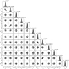 |
Fig. B.3. Posterior distributions of the surface brightness fits of the [CII] emission of the SGP38326 system, we fit the galaxies SGP38326-1 and SGP38326-2 simultaneously. We display the surface brightness at the effective radius in mJy/beam for the dust and mJy/beam km/s for the gas (Ie), the effective radius in kpc (Reff), the galactic centre in pixels (x0, y0), the ellipticity (ϵ), and the position angle in degrees (PA). The best values shown are the median followed by the lower and upper errors defined by the 16th and 84th percentiles, respectively. |
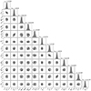 |
Fig. B.4. Posterior distributions of the surface brightness fits of the dust continuum emission of the SGP38326 system, we fit the galaxies SGP38326-1 and SGP38326-2 simultaneously. We display the surface brightness at the effective radius in mJy/beam for the dust and mJy/beam km/s for the gas (Ie), the effective radius in kpc (Reff), the galactic centre in pixels (x0, y0), the ellipticity (ϵ), and the position angle in degrees (PA). The best values shown are the median followed by the lower and upper errors defined by the 16th and 84th percentiles, respectively. |
Appendix C: Dynamical models
C.1. Dynamical models best-fit posteriors
Here we show the posterior distributions of the best-fit dynamical models obtained as described in Section 2.6. Our model contains five free parameters: stellar mass (M*), stellar effective radius (Reff, *), stellar Sérsic index (n), gas mass normalisation (gas_norm) and baryon fraction (fbar), which allows us to derive the virial mass of the CDM halo. We note that for BRI1335-0417, we fix the baryon fraction to the cosmological baryon fraction, therefore we only have four free parameters. The best-fit parameters reproduce the observed rotation curves as shown in Figure 3.
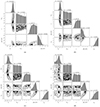 |
Fig. C.1. Corner plot with the posteriors of the best-fit dynamical models for the galaxies. The columns show: (i) the stellar mass in solar masses (logspace of M*); (ii) the effective radius of the stellar component in kpc (Reff, *); (iii) the Sérsic index of the stellar component (n); (iv) the normalisation of the gas (gas_norm); (v) the baryon fraction in logspace (fbar). Panels (a), (b), (c) and (d) are showing the results for the galaxies BRI1335-0417, J081740, SGP38326-1 and SGP38326-2, respectively. We note that for BRI1335-0417 we do not show the posterior for the baryon fraction as we fix it to the cosmological baryon fraction as discussed in Section 3.2. We show dashed lines for the best values followed by the upper and lower errors defined by the 50th, 16th and 84th percentiles, respectively. |
C.2. Further tests
We also performed a few more tests with different assumptions. Specifically, we test oversampling the rotation curves, both by modelling the kinematics with 3DBarolo with more rings and by interpolation the rotation curves, and we find that neither retrieve significantly different results. This implies that, to retrieve better constrains on the parameters considered, the main limiting factor in the model is the information in the shape of the rotation curves that can only be achieved with higher resolution data and/or with more extended rotation curves (i.e. higher S/R). Moreover, we considered models with the DM mass completely free and found that the baryon fraction becomes higher than the cosmological fraction, implying that the rotation curves of these galaxies can be reproduced without a CDM halo component, albeit likely overestimating the gas mass in order to reproduce the outer rotation. As mentioned in the main text, while the inner part of the rotation curve is sensitive to the stellar component, in the outer parts gas and DM tend to be degenerate.
Moreover, for BRI1335-0417, as explained in Section 3.2, we fixed the baryon fraction to the cosmological baryon fraction when modelling the rotation curve. The main drawback from undertaking the same assumptions used for the dynamical models of the other galaxies is that BRI1335-0417 has significantly lower circular speed with respect with its expected baryonic mass. Considering the disc inclination of 42° as derived in Roman-Oliveira et al. (2023), the rotation velocity of BRI1335-0417 goes from 180 km s−1 at 0.5 kpc to 124 km s−1 at 4.6 kpc. After performing the asymmetric drift correction, the circular speeds become 191 km s−1 in the centre and 153 km s−1 in the outskirts. If we use these circular speeds to roughly estimate the total mass at each radius then we find that the innermost ring encloses a mass of 4.2 × 10⁹ M⊙ and the outermost ring encloses a mass of 2.5 × 10¹⁰ M⊙.
If we take the CO luminosity observed for BRI1335-0417, presented in Table 1, and consider a conservative case with the lowest CO luminosity reported in Wagg et al. (2014), an αCO = 0.8 and a line ratio (J = 2-1/J = 1-0) of rl = 0.5 (Boogaard et al. 2020; Yang et al. 2017; Kamenetzky et al. 2016; da Cunha et al. 2013), BRI1335-0417 should have a gas mass of 2.92 ± 0.24 × 10¹⁰ M⊙. Just a simple comparison between the expected gas mass and the outer circular speed would imply that there is no room for neither the stellar component nor the CDM halo. Moreover, such a massive gas component could explain the outer rotation; however, given the shape of the gas exponential disc it could never reproduce the inner circular speeds. Therefore, for our fiducial model we considered the extreme case with the highest baryon fraction possible to derive the gas, stars and DM masses.
To explore whether we could potentially solve the discrepancy between the dynamical masses and the CO and stellar masses, in this Section we attempt at fitting the rotation curves with the disc inclination free and/or the NFW CDM halo concentration free. To include the inclination as a free parameter in our dynamical model we relate the circular speed Vc to the disc inclination by
 (C.1)
(C.1)
where, Vlos is the line-of-sight rotation velocity and i is the disc inclination. Therefore, if we were to consider a more face-on inclination of i = 30°, the rotation of at the innermost radius would increase to 256 km s−1 and the total mass enclosed within this radius would increase to 7.6 × 10⁹ M⊙.
We perform a dynamical model keeping the inclination free to vary uniformly in the range of 20° < i < 60° while also keeping the baryon fraction and the gas normalisation free to vary in the same range as used for the other galaxies. We find in this case that, despite potentially being able to increase the enclosed mass in the rotation curve to be modelled by decreasing the disc inclination, our dynamical model actually prefers higher inclinations (i = 50°). Therefore, the resulting model is somewhat similar to the fiducial model presented in the body of this paper, with a stellar mass of 1.7 × 10¹⁰ M⊙, 47% lower than the one obtained with our fiducial model. The best-fit baryon fraction is fbar = 0.12 and gas normalisation of gas_norm = 0.04, however, both of these values concentrate at the upper and lower edge of the prior range, respectively. This likely happens due to the flatness of the rotation curve of BRI1335-0417, since the innermost velocity is almost as high as the outskirt velocities any increase in the inner velocity translates to an even higher increase in the stellar mass. Ultimately, the main constrain is that the baryon fraction cannot exceed the cosmological baryon fraction.
Alternatively, we also test a dynamical model with a free DM concentration. In this case we keep the inclination fixed to 42 degrees, we use all the same priors for the remaining parameters and we let c200 vary uniformly between 1 and 10. In this case, we find a stellar mass of 2.4 × 10¹⁰ M⊙, a concentration c200 of 2.6 while the problems with the gas normalisation and baryon fraction remain.
All Tables
All Figures
|
Fig. 1. Surface brightness profiles of the gas distribution of the galaxies BRI1335−0417, J081740 and the SGP38326 system, respectively from top to bottom. Left panels: surface brightness map of the [CII] emission. The emission is shown as contours in turquoise for the data and magenta for the model. The contour levels follow levels of emission of 4σ, 8σ and 16σ, where σ is the RMS noise in the total map. We show the beam of the observations in the bottom left. Middle panel: residual map normalised by the RMS noise according to the colourbar shown. We show the centre of the best-fit model of each galaxy with a small cross. Right panel: 1D profile of the average gas emission in concentric ellipses (turquoise) and the best-fit Sérsic model (magenta), the dotted line shows the 4σ level above the noise. In the bottom panel we show the galaxies SGP38326−1 and SGP38326−2 together, as they have to be fitted simultaneously, and we mask the emission of SGP38326−3 in the bottom left corner. |
| In the text | |
|
Fig. 2. Surface brightness profile of the dust distribution of the galaxy J081740, the other galaxies are shown in Fig. B.1. Left panel: surface brightness map of the dust continuum. The emission is shown as contours in orange for the data and in violet for the best-fit model. The contour levels follow levels of emission of 4σ, 8σ and 16σ, where σ is the RMS noise in the total map. We show the beam of the observations in the bottom left. Middle panel: residual map normalised by the RMS noise according to the colourbar shown. We show the centre of the best-fit model of the galaxy with a small cross. Right panel: 1D profile of the average gas emission in concentric ellipses (orange) and the best-fit Sérsic model (violet), the black dotted line shows the 4σ level above the noise. |
| In the text | |
|
Fig. 3. Fiducial dynamical model for the galaxies. We show the measured circular speed, i.e. the rotation curve corrected for pressure support, as the blue shaded region. We also show the circular speed predicted by our model in black. The circular speed of the different mass components in the galaxies are shown as different shaded regions: stellar component (dash-dot line, orange), gas disc (dashed line, pink) and NFW CDM halo (dotted line, blue). In the case of BRI1335−0417, we fix the CDM halo to the cosmological baryon fraction. As explained in the main text, due to difficulties in breaking the degeneracy of the gas and DM contribution to the rotation curve we keep the CDM halo fixed to provide an upper limit on the baryon components. |
| In the text | |
|
Fig. 4. Stellar mass vs. star formation rate. Our galaxies are represented by coloured circles according to the legend. We also show some other galaxies in the literature at similar redshift (Rizzo et al. 2020, 2021; Faisst et al. 2020; Lelli et al. 2021). The black line shows the main sequence relation at z = 4.5 from Speagle et al. (2014), while the dashed and dotted lines show the starburst/main sequence boundary according to Rodighiero et al. (2011) and Rinaldi et al. (2022), respectively. |
| In the text | |
|
Fig. 5. Comparison of the observed gas velocity dispersion and star formation rate to expectations from analytical models from Krumholz et al. (2018). Left panel: different expectations from the model considering only gravitational instabilities as the driver of turbulence assuming fiducial parameters for high-z galaxies (solid lines). Right panel: different expectations from the model considering only stellar feedback as the driver of turbulence (solid lines). The models (solid lines) are colour-coded according to the maximum circular speed of the galaxies. We show our galaxies (Roman-Oliveira et al. 2023) and other resolved observations from the literature (Fraternali et al. 2021; Rizzo et al. 2021; Lelli et al. 2021) according to the legend. |
| In the text | |
|
Fig. 6. Observed turbulent energy in the discs (Eq. (9)) vs. maximum possible energy that can be injected in the ISM from SNII (Eq. (8)). We explore the possibility of a thin (0.3 kpc, thin ellipse) and a thick disc (1 kpc, thick ellipse). BRI1335−0417 is shown as open marker due to the uncertainties on the dynamical estimate of the gas mass. |
| In the text | |
|
Fig. 7. Baryonic Tully–Fisher relation (left panel) and the analogue of the Tully–Fisher relation for ETGs (right panel). Left panel: Baryonic mass and the circular speed on the flat region of the rotation curves of local disc galaxies and the best-fit BTFR relation in blue (Lelli et al. 2016b). Right panel: stellar masses and inner rotation of local ETGs with stellar kinematics in purple (Lelli et al. 2017) and with inner CO rotating discs in violet (Davis et al. 2016). We show the baryonic mass and external circular speed of our sample according to the legend, in the right panel, we also show their stellar mass (stars). |
| In the text | |
|
Fig. 8. Stellar-to-halo mass relation. We show the stellar-to-halo mass fraction on the y-axis versus the halo mass in the x axis. Our galaxies are shown as coloured circle markers according to the legend and the expected SHMR relation for central halos at 4.5 < z < 5.5 as a curve with 16th, 50th and 84th percentiles from Shuntov et al. (2022). |
| In the text | |
|
Fig. A.1. Comparison between the original rotation velocity obtained from the kinematic modelling (Vrot) and the circular speed after the asymmetric drift correction was applied with the method described in this Appendix (Vcirc) and the one obtained with 3DBAROLO (Vcirc, BB). |
| In the text | |
|
Fig. B.1. Surface brightness profiles of the dust distribution. Details are as described in the caption of Figure 1. |
| In the text | |
|
Fig. B.2. Posterior distributions of the surface brightness fits of the gas and dust distribution of the galaxies. Top left panel: [CII] emission of BRI1335-0417. Top right panel: Dust continuum emission of BRI1335-0417. Bottom left panel: [CII] emission of J081740. Bottom right panel: Dust continuum emission of J081740. All fits displayed have the Sérsic index fixed to 1.0, except for the dust distribution of BRI1335-0417 in which a free Sérsic index is preferred. We display the surface brightness at the effective radius in mJy/beam for the dust and mJy/beam km/s for the gas (Ie), the effective radius in kpc (Reff), the galactic centre in pixels (x0, y0), the ellipticity (ϵ), and the position angle in degrees (PA). The best values shown are the median followed by the lower and upper errors defined by the 16th and 84th percentiles, respectively. |
| In the text | |
|
Fig. B.3. Posterior distributions of the surface brightness fits of the [CII] emission of the SGP38326 system, we fit the galaxies SGP38326-1 and SGP38326-2 simultaneously. We display the surface brightness at the effective radius in mJy/beam for the dust and mJy/beam km/s for the gas (Ie), the effective radius in kpc (Reff), the galactic centre in pixels (x0, y0), the ellipticity (ϵ), and the position angle in degrees (PA). The best values shown are the median followed by the lower and upper errors defined by the 16th and 84th percentiles, respectively. |
| In the text | |
|
Fig. B.4. Posterior distributions of the surface brightness fits of the dust continuum emission of the SGP38326 system, we fit the galaxies SGP38326-1 and SGP38326-2 simultaneously. We display the surface brightness at the effective radius in mJy/beam for the dust and mJy/beam km/s for the gas (Ie), the effective radius in kpc (Reff), the galactic centre in pixels (x0, y0), the ellipticity (ϵ), and the position angle in degrees (PA). The best values shown are the median followed by the lower and upper errors defined by the 16th and 84th percentiles, respectively. |
| In the text | |
|
Fig. C.1. Corner plot with the posteriors of the best-fit dynamical models for the galaxies. The columns show: (i) the stellar mass in solar masses (logspace of M*); (ii) the effective radius of the stellar component in kpc (Reff, *); (iii) the Sérsic index of the stellar component (n); (iv) the normalisation of the gas (gas_norm); (v) the baryon fraction in logspace (fbar). Panels (a), (b), (c) and (d) are showing the results for the galaxies BRI1335-0417, J081740, SGP38326-1 and SGP38326-2, respectively. We note that for BRI1335-0417 we do not show the posterior for the baryon fraction as we fix it to the cosmological baryon fraction as discussed in Section 3.2. We show dashed lines for the best values followed by the upper and lower errors defined by the 50th, 16th and 84th percentiles, respectively. |
| In the text | |
Current usage metrics show cumulative count of Article Views (full-text article views including HTML views, PDF and ePub downloads, according to the available data) and Abstracts Views on Vision4Press platform.
Data correspond to usage on the plateform after 2015. The current usage metrics is available 48-96 hours after online publication and is updated daily on week days.
Initial download of the metrics may take a while.