| Issue |
A&A
Volume 671, March 2023
|
|
|---|---|---|
| Article Number | A44 | |
| Number of page(s) | 8 | |
| Section | Extragalactic astronomy | |
| DOI | https://doi.org/10.1051/0004-6361/202245202 | |
| Published online | 03 March 2023 | |
Dynamical signature of a stellar bulge in a quasar-host galaxy at z ≃ 6
1
Dipartimento di Fisica, Università di Trieste, Sezione di Astronomia, Via G.B. Tiepolo 11, 34131 Trieste, Italy
e-mail: This email address is being protected from spambots. You need JavaScript enabled to view it.
2
INAF – Osservatorio Astronomico di Trieste, Via G. Tiepolo 11, 34143 Trieste, Italy
3
IFPU – Institute for Fundamental Physics of the Universe, Via Beirut 2, 34151 Trieste, Italy
4
INAF – Osservatorio Astrofisico di Arcetri, Largo E. Fermi 5, 50125 Firenze, Italy
5
Institute of Astronomy, University of Cambridge, Madingley Road, Cambridge CB3 0HA, UK
6
Kavli Institute for Cosmology, University of Cambridge, Madingley Road, Cambridge CB3 0HA, UK
7
Department of Physics and Astronomy, University College London, Gower Street, London WC1E 6BT, UK
Received:
13
October
2022
Accepted:
17
January
2023
Abstract
We present a dynamical analysis of a quasar-host galaxy at z ≃ 6 (SDSS J2310+1855) using a high-resolution ALMA observation of the [CII] emission line. The observed rotation curve was fitted with mass models that considered the gravitational contribution of a thick gas disc, a thick star-forming stellar disc, and a central mass concentration, which is likely due to a combination of a spheroidal component (i.e. a stellar bulge) and a supermassive black hole (SMBH). The SMBH mass of 5 × 10⁹ M⊙, previously measured using the CIV and MgII emission lines, is not sufficient to explain the high velocities in the central regions. Our dynamical model suggests the presence of a stellar bulge with a mass of Mbulge ∼ 1010 M⊙ in this object, when the Universe was younger than 1 Gyr. To finally be located on the local MSMBH − Mbulge relation, the bulge mass should increase by a factor of ∼40 from z = 6 to 0, while the SMBH mass should grow by a factor of 4 at most. This points towards asynchronous galaxy-BH co-evolution. Imaging with the JWST will allow us to validate this scenario.
Key words: quasars: individual: SDSS J231038.88+185519.7 / galaxies: high-redshift / galaxies: kinematics and dynamics / galaxies: bulges / techniques: interferometric
© The Authors 2023
 Open Access article, published by EDP Sciences, under the terms of the Creative Commons Attribution License (https://creativecommons.org/licenses/by/4.0), which permits unrestricted use, distribution, and reproduction in any medium, provided the original work is properly cited.
This article is published in open access under the Subscribe to Open model. This email address is being protected from spambots. You need JavaScript enabled to view it. to support open access publication.
1. Introduction
The formation of central mass concentrations in galaxies, loosely defined as “bulges”, is still poorly understood. The main proposed scenarios for bulge formation involve major mergers, which produce spheroids with a large Sérsic index (Hernquist & Barnes 1991), and disc instabilities such as the formation of thick, buckling bars, which produce profiles with a smaller Sérsic index (the so-called pseudo-bulges; see e.g. Combes & Sanders 1981). The latter imply long timescales and therefore occur mainly at late cosmic times. At high redshift, disc instabilities manifest as turbulent discs hosting giant clumps that can coalesce to form bulges (Bournaud et al. 2007; Elmegreen et al. 2008). In addition, when a luminous active galactic nucleus (AGN) is present, its energy output in the form of radiation pressure on dust or shocks can contribute to the formation of a spheroidal component by triggering both galactic outflows and star formation (SF) (Ishibashi & Fabian 2014; Maiolino et al. 2017).
Recent observations of the [CII] line at 158 μm with the Atacama Millimeter/sub-millimeter Array (ALMA) revealed that stellar bulges can be in place up to z ≃ 5 (Lelli et al. 2021; Rizzo et al. 2021), when the Universe was only 1.2 Gyr old. This evidence is based on gas dynamics: the inner [CII] rotation velocities are very high (Vrot ≃ 300 − 400 km s−1) and show a Keplerian-like decline out to R ≃ 1 − 3 kpc, which can only be explained by a compact mass concentration. Similar rotation curves are indeed routinely observed in bulge-dominated galaxies at z ≃ 0 (e.g. Casertano & van Gorkom 1991; Noordermeer et al. 2007; Lelli et al. 2016). It is crucial to push these studies to even higher z to establish when the first bulges are formed and to better understand the co-evolution (or lack of it) with their central supermassive black holes (SMBHs).
We performed a dynamical decomposition of the rotation curve of Sloan Digital Sky Survey (SDSS) J231038.88+185519.7 (hereafter J2310) at z = 6.0031 (Tripodi et al. 2022; Wang et al. 2013), based on high-resolution ALMA observations. J2310 was first identified as a quasi-stellar object (QSO) in SDSS (Jiang et al. 2006; Wang et al. 2013) and is one of the most luminous QSOs known in the optical and far-infrared bands, with a bolometric luminosity of Lbol = 9.3 × 10¹³ L⊙.
Bischetti et al. (2022) reported evidence for an AGN-driven ionised-gas wind traced by ultra-violet (UV) broad absorption lines. The host galaxy is characterised by a star formation rate (SFR) in the range ∼1200–2400 M⊙ yr−1 (Shao et al. 2019; Tripodi et al. 2022) that occurs in a regularly rotating gaseous disc without evidence of interactions or mergers.
Tripodi et al. (2022) presented a tilted-ring modelling of the [CII] emission that resulted in a flat rotation curve and derived a disc inclination i ≃ 25° and a dynamical mass 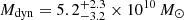 . They interpreted the high velocities seen near the galactic centre as due to a [CII] outflow. An alternative possible explanation for the high-velocity [CII] emission is fast rotation due to the presence of a central mass concentration. In this study, we investigate whether a bulge can indeed be the most likely cause for the velocity enhancement in the innermost region of J2310 by modelling the rotation curve with different mass models.
We adopted a ΛCDM cosmology from Planck Collaboration XIII (2016): H0 = 67.7 km s−1 Mpc−1, Ωm = 0.308 and ΩΛ = 0.692. Thus, the angular scale is 5.84 kpc arcsec−1 at z = 6. We analysed the same [CII] cube as described in Tripodi et al. (2022). It has a spatial resolution of (0.17 × 0.15) arcsec2, which corresponds to ∼0.9 kpc at the redshift of the QSO.
2. Analysis and results
2.1. [CII] rotation curve
We derived a new rotation curve of J2310 using the software 3DBarolo (Di Teodoro & Fraternali 2015), improving the preliminary kinematic modelling of Tripodi et al. (2022). 3DBarolo directly fits disc models to the 3D cube and considers the effects of spectral and spatial resolution (beam smearing). The galaxy is divided into a series of rings, each of which is described by nine parameters: coordinates of the kinematic centre (x0, y0), position angle (PA), inclination (i), vertical thickness (z0), systemic velocity (Vsys), rotation velocity (Vrot), radial velocity (Vrad), and velocity dispersion (σv). For (x0, y0), Vsys, and i, we adopted the same estimates as in Tripodi et al. (2022). We fixed z0 to 300 pc, but this parameter has a negligible effect on our results because our spatial resolution is ∼900 pc and the disc is nearly face-on (i ≃ 25°). Since the kinematic major axis is perpendicular to the minor axis, we fixed the radial velocity to zero. With respect to Tripodi et al. (2022), we changed the PA to 195° because the data-model residual maps in their Fig. 8 suggest that their value of 200° was slightly overestimated (see Warner et al. 1973). We also changed the radial sampling to avoid aggressive over-sampling; we used four rings spaced by 0.07 arcsec, which corresponds to 0.409 kpc. In order to minimise the impact of the outflowing material on our results, we cropped the [CII] cube considering the velocity range [−290, +270] km s−1. This excludes the blue and red wings seen in the spatially integrated [CII] spectrum (see Fig. 2 in Tripodi et al. 2022). We then ran 3DBarolo with vrot and σv as free parameters. 3DBarolo provides asymmetric uncertainties (δ+, δ−), corresponding to a variation of 5% in the residual from the global minimum. We treated them as 1σ uncertainties and took the mean value of (δ+, δ−) to compute symmetric uncertainties that were used in subsequent rotation-curve fits.
Figure 1 shows position-velocity (PV) diagrams along the major and minor axes of the disc. In Tripodi et al. (2022), the comparison between disc model and observations showed a mismatch at line-of-sight velocities VLOS of ±300 km s−1 along both the major and minor axes. This mismatch was interpreted as due to the gas outflow. The overall symmetry of the PV diagrams, however, may suggest that the high-velocity emission is associated with fast rotation. With the new rotation curve, the central mismatch at ≳300 km s−1 has now decreased along both axes, indicating that the new model fits the data better.
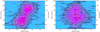 |
Fig. 1. PV diagrams of the [CII] emission line along the kinematic major axis (left panel) and kinematic minor axis (right panel), performed with 3DBarolo. Contours are at 2, 3, 6, and 12σ, with σ = 0.22 mJy beam−1, for the data (solid black lines) and the best-fit model (dashed orange lines). Yellow stars show the projected rotation curve modelled by 3DBarolo. |
The rotation curve shown in Fig. 1 is approximately flat, with a slight increase towards the centre. The average deprojected rotation velocity is ∼365 km s−1, similar to what was found in Tripodi et al. (2022). The velocity dispersion profile (not shown) increases towards the centre and reaches σgas ≃ 80 km s−1, with an average value of ∼70 km s−1. This gives Vrot/σgas ≃ 5, so that the disc is rotation supported and the observed rotation velocities are a good tracer of the circular velocity of a test particle in the equilibrium gravitational potential. The circular velocity approximately goes as  , therefore corrections for pressure support are a few km s−1 at most and are therefore negligible.
2.2. Mass models
We used the observed rotation curve to constrain the mass distribution within the galaxy. We considered three to four mass contributions: a gaseous disc, a stellar disc, an SMBH, and possibly, a stellar bulge. The model circular velocity at radius R is then given by
 (1)
(1)
where  are dimensionless parameters of the order of one (with j = gas, disc, bulge). Essentially, for numerical convenience, we normalised the gravitational contributions to a mass of 1010 M⊙ and scaled them using Yj. The gaseous and stellar disc were both modelled as thick discs with a radial density profile given by the observed [CII] and dust surface brightness profiles, respectively (following Lelli et al. 2021). For the vertical density profile, we assumed an exponential function with a fixed scale height. The stellar bulge was modelled as a spherical projected De Vaucouleurs profile with a fixed effective radius of 0.07 arcsec (∼409 pc). This is the maximum effective radius allowed by the data, so that our bulge model maximises the difference between an extended mass distribution and a point source. The SMBH was modelled as a point mass. A detailed description of our assumptions is given in Appendix A.
The masses of the stellar and gas discs are degenerate because their velocity contributions have a similar shape, which rises with radius. To break this degeneracy, we imposed a tight prior on Ygas by adopting a gas mass of 4.4 × 10¹⁰ M⊙ (Feruglio et al. 2018; Li et al. 2020; Tripodi et al. 2022, for more details see Appendix A). Similarly, the masses of bulge and SMBH are degenerate because their velocity contributions declines with radius. This occurs because the spatial resolution of the rotation curve cannot discern a central point source from a more extended central mass concentration. To break this degeneracy, we fixed the SMBH mass to 5 × 10⁹ M⊙ (Mazzucchelli et al., in prep.; Bischetti et al. 2022). This estimate comes from X-shooter spectroscopy of the MgII and CIV lines, which has a high signal-to-noise ratio and assumes the z ≃ 0 scaling relations provided by Vestergaard & Osmer (2009), Vestergaard & Peterson (2006), and Coatman et al. (2017).
Depending on the chosen model, we therefore had three or four free parameters: the inclination i of the [CII] disc that changes the observed rotation velocities as Vobssin(i), and two or three parameters among Ygas, Y*disc, and Ybulge. The best-fitting parameters were determined using a Markov chain Monte Carlo (MCMC) method in a Bayesian context. We adopted a Gaussian prior on i and lognormal priors on the Yj parameters. The choices for the central and standard deviation values for all the fitting parameters are listed in Table 1.
MCMC priors.
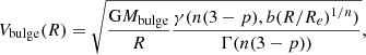
To assess whether the bulge is a truly essential component, we started with a conservative model that considered only stellar disc, gas disc, and SMBH with a fixed mass. Figure 2 (model A, left panel) shows that this model misses the first point of the rotation, and the inclination is pushed up to 38° (more than 2.5σ from the prior value) to decrease the rotation velocities as much as possible. When we instead consider a model in which the BH mass is entirely free, we obtain a good result, but the required BH mass is higher than the expected value derived from the MgII line by a factor of 2 (i.e. MBH = 1.1 ± 0.4 × 10¹⁰ M⊙). This high mass is still within the systematic uncertainties of ∼0.3 dex associated with BH masses from MgII measurements (Vestergaard & Peterson 2006). An increase in the BH mass of a factor of 2 would therefore be able to remove the need for an additional central stellar concentration. However, this scenario seems very unlikely according to galaxy formation models (see Sect. 3 and Fig. 3).
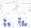 |
Fig. 2. Results for mass models. Top panels: Two different mass models are fitted to the observed rotation curve (black squares): no bulge and fixed BH mass (A), bulge and fixed BH mass (B). The best-fitting model (solid black line) is the sum of the contributions from the stellar disc (dashed blue line), the cold gas disc (dotted green line), the BH (dotted purple line), and the stellar bulge (when present; dot-dashed red line). The different values of the rotation velocities in models A and B are due to different best-fitting values for the inclination: i = 38 ± 2° for model A and i = 26 ± 4° for model B. Bottom panels: Posterior distributions of the fitting parameters for models A and B. |
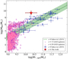 |
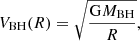
Fig. 3. Black hole mass vs. spheroid stellar mass. Comparison between the z = 0 sample of early-type galaxies from Sahu et al. (2019) (blue squares) and our results for the z = 6 QSO J2310 (red star). The green line is the best-fit relation for the z = 0 sample. Its scatter (green shadowed region) is taken from Sahu et al. (2019). The purple and pink triangles are the z = 5.72 and z = 6.20 galaxies, respectively, that were modelled by the GAEA-F06 run (Fontanot et al. 2020). |
Finally, we considered a mass model that included both an SMBH with a fixed mass and a bulge component. Figure 2 (model B, right panel) shows that this model reproduces the observed rotation curve well and preserves the prior value of i ≃ 25°. The best-fitting values are reported in Table 2. We find a bulge mass of ∼1.7 × 10¹⁰ M⊙ that implies Mbulge ≃ 0.27 × Mbaryon, where Mbaryon = Mgas + M*disc + Mbulge. The best-fit mass also implies an effective surface mass density Σeff ≃ 3 × 10⁴ M⊙ pc−2, which is consistent with that of the most compact spheroids at z ≃ 0. It seems unlikely that such a compact mass component can be in the form of [CII]-dark or CO-dark gas because it should lead to a strong central enhancement of star formation that is not visible in the sub-millimeter continuum map. At larger radii, however, the gas contribution becomes strong, and the galaxy has Mgas ≃ 0.67 × Mbaryon; this result is largely driven by the tight prior on the gas mass.
MCMC results for mass model B.
Recently, Shao et al. (2022) presented a similar analysis of the rotation curve of J2310, using a razor-thin gas disc and a single spherical stellar component. They obtained a stellar mass of 5.8 × 10⁹ M⊙ when they fixed the BH mass to the value of 1.8 × 10⁹ that was derived from the analysis of the CIV emission line (Feruglio et al. 2018). Our mass models are different from theirs because we distinguish between a star-forming stellar disc and a spherical bulge, which is crucial to locate J2310 on the BH-bulge scaling relation (see Sect. 3). In addition, in our models, the gas and stellar discs have a realistic finite thickness. Importantly, Shao et al. (2022) concluded that they measured the dynamical mass of a black hole for the first time at z ≃ 6, whereas we find that the BH mass and bulge mass are degenerate. To break this degeneracy, the BH mass must be fixed using independent information, given the low spatial resolution of the ALMA data (∼900 pc). For comparison, dynamical BH mass measurements in AGN-host galaxies at z ≃ 0 require spatial resolutions better than 100 pc (e.g. Combes et al. 2019; Lelli et al. 2022). The observed rotation curve of J2310 clearly indicates a central mass concentration, but the ALMA data themselves cannot determine whether this is entirely due to a BH, a stellar bulge, or a combination of both. In our view, the latter scenario is the most likely.
3. Discussion and conclusions
Our dynamical analysis suggests the presence of a central compact mass component in J2310. This component is composed of an SMBH and a stellar bulge with similar masses of the order of ∼1.7 × 10¹⁰ M⊙. Two crucial questions that arise from this result are first, how a bulge of ∼ 1010 M⊙ was able to form in less than 1Gyr, and second, what the implications of our results are for the overall picture of SMBH-galaxy co-evolution.
As we discussed in Sect. 1, several mechanisms have been proposed for the formation of galaxy bulges: disc instabilities (Combes & Sanders 1981; Bournaud et al. 2007), major mergers (Toomre et al. 1977; Hernquist & Barnes 1991), SF in AGN driven outflows (Ishibashi & Fabian 2014), and direct dissipative collapse (Eggen et al. 1962; Sandage 1990). For J2310, disc instabilities can probably be ruled out because these secular processes occur on long timescales (∼3–5 Gyr), while the age of the Universe at z ≃ 6 is only ∼900 Myr in the adopted cosmology. All the other mechanisms appear viable, however. The host galaxy of J2310 does not show any evidence of ongoing mergers based on the high-resolution ALMA data that are available to date, but the orbital time at the last measured point of the rotation curve is only 26 Myr, which means that the [CII] disc may relax in just ∼100 Myr (about four revolutions) after a violent event. This implies that the last potential merger between (proto-)galaxies with masses of a few times 109 M⊙ must have occurred at z > 6.5.
Feedback from AGN in the form of large-scale outflows driven by the radiation pressure on dust or by shock propagation may trigger the formation of new stars at outer radii, leading to the development of extended stellar envelopes (Ishibashi & Fabian 2014). Observational evidence supporting this scenario was provided by Maiolino et al. (2017), who found that SF can occur within galactic outflows where the newly formed stars follow ballistic trajectories that can fall back in the potential and thus form a spheroidal component. In this scenario, the accreting BH triggers SF and contributes to the formation of the stellar bulge. This scenario may form extended and diffuse bulges, while in J2310, we find evidence for a compact mass concentration with a high effective surface density.
Regarding the BH-galaxy co-evolution, for J2310, Tripodi et al. (2022) found that the SMBH growth efficiency is ∼50% lower than that of its host galaxy. This suggests that AGN feedback effectively slows down the accretion onto the SMBH, while the host galaxy is still growing fast. The onset of significant BH feedback hampering BH growth marks the transition from a phase of BH dominance to a phase of symbiotic growth of the BH and the galaxy (Volonteri 2012). In Fig. 3, we locate J2310 on the local MBH − Mbulge relation (green region) and the local observational data (blue squares) from Sahu et al. (2019). J2310 deviates from the z ≃ 0 relation because it has MBH ≃ 0.3Mbulge, while in local galaxies, MBH ≃ (0.01 − 0.1)×Mbulge. When we assume that the BH of J2310 evolves into one of the most massive BH at z = 0 (MBH ≃ 2 × 10¹⁰ M⊙), it can grow in mass by only a factor of 4 during ∼13 Gyr, while the bulge should grow by a factor of ∼40 to reach a mass around 1011.8 M⊙ at z ≃ 0. This suggests an asynchronous growth between SMBH and bulges. Moreover, the available molecular gas in J3210 is estimated to be ∼4 × 10¹⁰ M⊙. To reach a stellar mass of ∼1011.8 M⊙ at z ≃ 0, the galaxy needs to accrete a comparable amount of mass (in gas or directly in stars) over ∼13 Gyr, giving an average mass accretion rate of ∼40 M⊙ yr−1. For example, if the galaxy continues to form stars with SFR ≃ 103 M⊙ yr−1, a stellar mass of (5 − 10)×1011 M⊙ can be formed in only 0.5–1.0 Gyr (by z ≃ 3.5 − 4.0), but would then require a mass-accretion rate comparable to the SFR. In any case, our result seems to highlight the absence of any symbiotic growth between the SMBH and the host galaxy at high redshift; it appears that the SMBH firstly experiences a phase of rapid and intense growth (reaching up to 5 × 10⁹ M⊙ in less than 1 Gyr), followed by the growth of the galaxy.
Finally, we compared our result with theoretical predictions of the GAlaxy Evolution and Assembly (GAEA) model (in detail the GAEA-F06 run, Fontanot et al. 2020), to shed light on the mechanism leading to the formation of this bulge. This semi-analytic model includes two different channels of bulge formation (i.e. galaxy mergers and disc instabilities; see e.g. De Lucia et al. 2011): both physical processes also help bringing cold gas onto the central SMBH, thus feeding accretion and AGN events. In Fig. 3 we also show the distribution of model galaxies1 in the MBH − Mbulge plane (purple and pink triangles) compared with a local z ∼ 0 sample (Sahu et al. 2019). From the comparison, we can conclude that (a) GAEA-F06 predicts a relevant population of Mbulge > 109 M⊙ bulges in high-z galaxies despite the relatively young cosmic epoch, and (b) the scatter around the z ∼ 6 MBH − Mbulge relation is much larger than in the local Universe. This is likely due to the different contribution of the two bulge-forming channels (mergers and disc instabilities) to the corresponding SMBH accretion (see Fontanot et al. 2020): in this interpretation, at fixed Mbulge, higher (lower) MBH corresponds to sources that experienced more mergers (disc instabilities). We plan to further test this hypothesis in forthcoming work. We verified that GAEA predicts that all objects lying above the MBH − Mbulge relation at z ∼ 6 converge towards the z ∼ 0 relation at later times. Nonetheless, none of the model galaxies reaches z ∼ 6 MBH as high as the one estimated for J2310, which thus represents the main difference between data and model predictions.
A robust interpretation of our results is strongly dependent on the accuracy of the determination of the physical quantities at play. In particular, to be able to precisely quantify the mass of the central bulge, we would need a [CII] observation with higher resolution. To verify this, we simulated a rotation curve derived from an observation with a resolution of ∼0.05 arcsec, that is, an improvement of a factor of ×3 (linear) compared to our current resolution, and we find that this observation would allow us to constrain the bulge mass to within an uncertainty of 30% (for further details, see Appendix B). This observation would be feasible with ALMA.
The GAEA-F06 realisation has been defined on merger trees extracted from the Millennium Simulation. We considered model galaxies in the two snapshots closer to the estimated J2310 redshift, z = 6.20 and z = 5.72.
Acknowledgments
We thank the referee for the useful suggestions. RT thanks Marta Molero for the insightful discussions. This paper makes use of the following ALMA data: ADS/JAO.ALMA#2019.1.00661.S. ALMA is a partnership of ESO (representing its member states), NFS (USA) and NINS (Japan), together with NRC (Canada), MOST and ASIAA (Taiwan) and KASI (Republic of Korea), in cooperation with the Republic of Chile. The Joint ALMA Observatory is operated by ESO, AUI/NRAO and NAOJ. RT acknowledges financial support from the University of Trieste. RT, CF, FF, MB acknowledge support from PRIN MIUR project “Black Hole winds and the Baryon Life Cycle of Galaxies: the stone-guest at the galaxy evolution supper”, contract #2017PH3WAT. RM acknowledges ERC Advanced Grant 695671 QUENCH, and support from the UK Science and Technology Facilities Council (STFC). RM also acknowledges funding from a research professorship from the Royal Society. The authors thank Pierluigi Monaco for his helpful suggestions. This paper makes extensive use of python packages, libraries and routines, such as numpy, scipy and astropy. Facilities: ALMA. Software: CASA (v5.1.1-5, McMullin et al. 2007), 3DBarolo (Di Teodoro & Fraternali 2015).
References
- Accurso, G., Saintonge, A., Catinella, B., et al. 2017, MNRAS, 470, 4750 [NASA ADS] [Google Scholar]
- Bershady, M. A., Verheijen, M. A. W., Swaters, R. A., et al. 2010, ApJ, 716, 198 [NASA ADS] [CrossRef] [Google Scholar]
- Bischetti, M., Feruglio, C., D’Odorico, V., et al. 2022, Nature, 605, 244 [NASA ADS] [CrossRef] [Google Scholar]
- Bolatto, A. D., Wolfire, M., & Leroy, A. K. 2013, ARA&A, 51, 207 [CrossRef] [Google Scholar]
- Bournaud, F., Elmegreen, B. G., & Elmegreen, D. M. 2007, ApJ, 670, 237 [Google Scholar]
- Carilli, C. L., & Walter, F. 2013, ARA&A, 51, 105 [NASA ADS] [CrossRef] [Google Scholar]
- Casertano, S. 1983, MNRAS, 203, 735 [NASA ADS] [CrossRef] [Google Scholar]
- Casertano, S., & van Gorkom, J. H. 1991, AJ, 101, 1231 [NASA ADS] [CrossRef] [Google Scholar]
- Coatman, L., Hewett, P. C., Banerji, M., et al. 2017, MNRAS, 465, 2120 [Google Scholar]
- Combes, F., & Sanders, R. H. 1981, A&A, 96, 164 [NASA ADS] [Google Scholar]
- Combes, F., García-Burillo, S., Audibert, A., et al. 2019, A&A, 623, A79 [NASA ADS] [CrossRef] [EDP Sciences] [Google Scholar]
- De Lucia, G., Fontanot, F., Wilman, D., & Monaco, P. 2011, MNRAS, 414, 1439 [NASA ADS] [CrossRef] [Google Scholar]
- Di Teodoro, E. M., & Fraternali, F. 2015, MNRAS, 451, 3021 [Google Scholar]
- Eggen, O. J., Lynden-Bell, D., & Sandage, A. R. 1962, ApJ, 136, 748 [NASA ADS] [CrossRef] [Google Scholar]
- Elmegreen, B. G., Bournaud, F., & Elmegreen, D. M. 2008, ApJ, 688, 67 [NASA ADS] [CrossRef] [Google Scholar]
- Feruglio, C., Fiore, F., Carniani, S., et al. 2018, A&A, 619, A39 [NASA ADS] [CrossRef] [EDP Sciences] [Google Scholar]
- Fontanot, F., De Lucia, G., Hirschmann, M., et al. 2020, MNRAS, 496, 3943 [CrossRef] [Google Scholar]
- Genzel, R. 2017, in Disk Instabilities Across Cosmic Scales, 5 [Google Scholar]
- Genzel, R., Price, S. H., Übler, H., et al. 2020, ApJ, 902, 98 [NASA ADS] [CrossRef] [Google Scholar]
- Hernquist, L., & Barnes, J. E. 1991, Nature, 354, 210 [NASA ADS] [CrossRef] [Google Scholar]
- Ishibashi, W., & Fabian, A. C. 2014, MNRAS, 441, 1474 [NASA ADS] [CrossRef] [Google Scholar]
- Jiang, L., Fan, X., Hines, D. C., et al. 2006, AJ, 132, 2127 [NASA ADS] [CrossRef] [Google Scholar]
- Lelli, F., McGaugh, S. S., & Schombert, J. M. 2016, AJ, 152, 157 [Google Scholar]
- Lelli, F., Di Teodoro, E. M., Fraternali, F., et al. 2021, Science, 371, 713 [Google Scholar]
- Lelli, F., Davis, T. A., Bureau, M., et al. 2022, MNRAS, 516, 4066 [NASA ADS] [CrossRef] [Google Scholar]
- Li, J., Wang, R., Riechers, D., et al. 2020, ApJ, 889, 162 [NASA ADS] [CrossRef] [Google Scholar]
- Lima Neto, G. B., Gerbal, D., & Márquez, I. 1999, MNRAS, 309, 481 [Google Scholar]
- Maiolino, R., Russell, H. R., Fabian, A. C., et al. 2017, Nature, 544, 202 [Google Scholar]
- McMullin, J. P., Waters, B., Schiebel, D., Young, W., & Golap, K. 2007, in Astronomical Data Analysis Software and Systems XVI, eds. R. A. Shaw, F. Hill, & D. J. Bell, ASP Conf. Ser., 376, 127 [Google Scholar]
- Noordermeer, E., van der Hulst, J. M., Sancisi, R., Swaters, R. S., & van Albada, T. S. 2007, MNRAS, 376, 1513 [NASA ADS] [CrossRef] [Google Scholar]
- Pearson, W. J., Wang, L., Hurley, P. D., et al. 2018, A&A, 615, A146 [NASA ADS] [CrossRef] [EDP Sciences] [Google Scholar]
- Planck Collaboration XIII. 2016, A&A, 594, A13 [NASA ADS] [CrossRef] [EDP Sciences] [Google Scholar]
- Rizzo, F., Vegetti, S., Powell, D., et al. 2020, Nature, 584, 201 [Google Scholar]
- Rizzo, F., Vegetti, S., Fraternali, F., Stacey, H. R., & Powell, D. 2021, MNRAS, 507, 3952 [NASA ADS] [CrossRef] [Google Scholar]
- Sahu, N., Graham, A. W., & Davis, B. L. 2019, ApJ, 876, 155 [NASA ADS] [CrossRef] [Google Scholar]
- Sandage, A. 1990, JRASC, 84, 70 [NASA ADS] [Google Scholar]
- Shao, Y., Wang, R., Carilli, C. L., et al. 2019, ApJ, 876, 99 [NASA ADS] [CrossRef] [Google Scholar]
- Shao, Y., Wang, R., Weiss, A., et al. 2022, A&A, 668, A12 [Google Scholar]
- Terzić, B., & Graham, A. W. 2005, MNRAS, 362, 197 [CrossRef] [Google Scholar]
- Toomre, A. 1977, in Evolution of Galaxies and Stellar Populations, eds. B. M. Tinsley, D. C. Larson, & R. B. Gehret, 401 [Google Scholar]
- Tripodi, R., Feruglio, C., Fiore, F., et al. 2022, A&A, 665, A107 [NASA ADS] [CrossRef] [EDP Sciences] [Google Scholar]
- Vestergaard, M., & Osmer, P. S. 2009, ApJ, 699, 800 [Google Scholar]
- Vestergaard, M., & Peterson, B. M. 2006, ApJ, 641, 689 [Google Scholar]
- Vogelaar, M. G. R., & Terlouw, J. P. 2001, in Astronomical Data Analysis Software and Systems X, eds. F. R. Harnden, Jr., F. A. Primini, & H. E. Payne, ASP Conf. Ser., 238, 358 [NASA ADS] [Google Scholar]
- Volonteri, M. 2012, Science, 337, 544 [NASA ADS] [CrossRef] [Google Scholar]
- Wang, R., Wagg, J., Carilli, C. L., et al. 2013, ApJ, 773, 44 [Google Scholar]
- Warner, P. J., Wright, M. C. H., & Baldwin, J. E. 1973, MNRAS, 163, 163 [NASA ADS] [Google Scholar]
Appendix A: Details of the mass models
In this section, we describe the mass models we adopted in more detail. The gravitational contribution of the gas disc was computed using the task Rotmod in the GIPSY software (Vogelaar & Terlouw 2001). It numerically solves the equation from Casertano (1983) for a truncated disc of finite thickness. For the radial column density distribution, we used the observed [CII] surface brightness profile as input, which is close to exponential. For the vertical density distribution, we assumed an exponential profile with a scale height z0 = 160 pc. This is motivated by the scaling relation between scale length and scale height that is observed in edge-on disc galaxies at z = 0 (e.g. Bershady et al. 2010), but the precise value of z0,gas has a very minor effect on our results. In the limiting case of a razor-thin exponential disc (i.e. z0,gas = 0), our results would vary within 15%, which is well within our current uncertainties on the fitted quantities. We did not use the CO(6-5) surface brightness emission (Tripodi et al. 2022) because it was derived from data with lower resolution (∼0.5 arcsec; Feruglio et al. 2018), therefore the observed CO surface brightness profile is more sparsely sampled than the [CII] profile. For J2310, precise determinations for Mgas were obtained using the CO(6-5) emission line together with the CO spectral line energy distribution (Feruglio et al. 2018; Li et al. 2020; Tripodi et al. 2022); we used the value of 4.4 × 10¹⁰ M⊙ as a tight prior on Mgas. This estimate was derived by fitting the spectral line energy distribution of high-J CO lines and assuming a CO-to-H2 conversion factor αCO = 0.8 M⊙ (K km s−1 pc−2)−1, which is currently thought to be most appropriate for QSO-host galaxies (Carilli & Walter 2013). Systematic uncertainties on αCO in starburst AGN-host galaxies can be large even at z ≃ 0 (Bolatto et al. 2013), but there is mounting evidence that their αCO are systematically smaller than those of Milky-Way-like galaxies (Accurso et al. 2017; Pearson et al. 2018; Lelli et al. 2022). We associate a 25% uncertainty with Mgas. This tight prior is necessary to break a degeneracy between Ygas and Y*disc that arises because gas disc and stellar disc provide velocity contributions with a similar shape. The actual gas mass may be more uncertain than assumed here, but this assumption mostly impacts the relative masses of the stellar and gas discs but leaves our conclusions on the central mass concentration unaltered.
The gravitational contribution of the star-forming stellar disc was computed in a similar way as for the gas disc. For the radial column density profile, we used the surface brightness profile from the ALMA sub-millimeter continuum map, which traces hot dust heated by young stars. The sub-millimeter emission can be used as a proxy for the distribution of the stellar disc because dust absorbs UV radiation from young stars and re-emits it at far-infrared wavelengths (Lelli et al. 2021). The continuum surface brightness profile in Tripodi et al. (2022) is well described by an exponential profile with scale length R*disc = 0.71 kpc, which further supports the use of dust emission as a proxy for the star-forming disc. For the distribution of the vertical surface density, we assumed an exponential profile with z0 ≃ 160 pc as for the gas disc, but this assumption has a very minor effect on our results.
The stellar bulge was modelled as a spherical projected Sérsic profile, so that its gravitational contribution is given by (Lima Neto et al. 1999; Terzić & Graham 2005)
 (A.1)
(A.1)
where Mbulge is the stellar bulge mass, Re is the effective radius, n is the Sérsic index, b = 2n − 1/3 + 0.009876/n for 0.5 < n < 10, γ and Γ are the incomplete and complete gamma function, respectively, and p = 1.0 − 0.6097/n + 0.05563/n2 for 0.6 < n < 10 and 10−2 ≤ R/Re ≤ 103. We fixed n = 4 (a De Vaucouleurs profile) and set Re = 0.07 arcsec ∼409 pc, that is, ∼beam size/2. Lower values of Re would not significantly change the contribution of the bulge in the centre, making it very similar to a point source. In principle, Re could be determined from high-resolution rest-frame optical and/or near-infrared images after subtracting the QSO contribution, but data like this are currently not available. Alternatively, Re may be set as a free parameter in our model, but we do not have enough data points in the rotation curve to fit more than four parameters.
The SMBH gives the velocity contribution of a point source,
 (A.2)
(A.2)
where MBH is the black mass. In our models, MBH could be either a free or a fixed parameter. In the latter case, it was fixed to MBH = 5.0 × 10⁹ M⊙, derived from the MgII emission line profile (Mazzucchelli in prep., Tripodi et al. 2022).
In our modelling, we did not consider the contribution of a dark matter (DM) component for several reasons: (1) in general, the DM contribution in massive galaxies becomes important in the outer regions, beyond the stellar disc, because it has a rising trend with the radius. This component would therefore not affect our main results about the central mass component. (2) In our specific case, the rotation curve was measured out to a radius of just 1.7 kpc, within which the gravitational potential is likely dominated by baryons (in analogy to star-forming galaxies at slightly lower redshifts; e.g. Genzel 2017; Genzel et al. 2020; Rizzo et al. 2020, 2021; Lelli et al. 2021). (3) Our four data points do not enable us to fit for additional free parameters, which would be required if we were to add a DM component. Therefore, we opted for the simplest physically motivated mass model with the smallest number of free parameters.
Appendix B: Simulated observation
In this section, we evaluate the advantages of a very high resolution ALMA observation of the [CII] emission line in the QSO J2310. The goal of this observation would be to obtain an accurately sampled rotation curve, derived from a dynamical analysis of the [CII] emission line. This would allow us to quantify the contribution of the bulge with higher precision.
The parameters that describe the behaviour of a bulge in the rotation curve are the bulge mass, Mbulge, the Sérsic index, n, and the effective radius, Re (see Sect. 2.2). In order to constrain these three parameters, we would require a resolution that is of the order of ∼Re/2. For our QSO at z ∼ 6, we adopted Re = 0.07 arcsec (see Sect. 2.2), therefore the required resolution is 0.05 arcsec, that is, three times lower than the resolution of the real observation we analysed in this work. First, we simulated a rotation curve that we would obtain using an observation with a resolution of 0.05 arcsec and given the results obtained in Sect. 2.2. Secondly, we fit this simulated rotation curve using the mass models described in Appendix B, in order to assess the improvement achieved with higher-resolution data.
In Sect. 2.2 and Sect. 3, we concluded that the best model able to describe the shape of our observed rotation curve is model B, considering the contributions of a gaseous disc, a stellar disc, a BH, and a bulge. In order to build the simulated rotation curve, we fixed the mass of the components and the inclination at the values reported in Table 2, and also Re = 0.07, n = 4. We considered two points per resolution element and therefore obtained 11 simulated data points equally spaced by 0.025 arcsec (see the black squares in the left panel of Figure B.1). We fit the simulated data set running an MCMC with five free parameters, Ygas, Y*disc, Ybulge, Re, n, and a fixed BH mass (MBH = 5 × 10⁹ M⊙). We adopted lognormal priors for the dimensionless mass parameters and Gaussian priors for Re and n. In particular, we used a tight prior on the gas mass (log(Ygas)prior = 0.64 ± 0.11), and the priors on log(Y*disc), log(Ybulge),Re, n were centred near the values obtained (or fixed) for model B (see Table 2) with standard deviations of 0.5, 0.5, 0.05, and 0.5. The best-fitting model is shown in the left panel of Figure B.1 as a solid black curve together with its four components (gas in green, stellar disc in blue, BH in purple, and bulge in red). The corner plot and the numerical results are presented in the right panel of Figure B.1 and Table B.1. The values of the best-fitting parameters agree very well with the expected values of model B, and the uncertainties are decreased from 20% to 10% for the gas mass and from 70% to 30% for the bulge mass. The uncertainty on the stellar disc mass is still high because this contribution has a strong degeneracy with the gas contribution, and therefore an independent measurement of the stellar disc mass would be required in order to place a tighter prior on Y*disc and reduce its uncertainty. Similarly, a better estimation of Re would be obtained by a direct measurement of the bulge, for instance with the JWST. Nevertheless, the precision on the estimate of the bulge mass that is achieved with a very high resolution ALMA observation is four times higher than the precision obtained with our real observation. This result supports the request for a very high resolution (0.05 arcsec) ALMA observation, which has been proven to be able to place a tight constraint on the bulge mass.
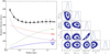 |
Fig. B.1. Results for the rotation curve of the simulated observation. Left: Best-fitting model for the simulated rotation curve. The best-fitting model (solid black line) is the sum of the contributions from the stellar disc (dashed blue line), the cold gas disc (dotted green line), the stellar bulge (dot-dashed red line), and the BH (dotted purple line). Right: Corner plot showing the four-dimensional posterior probability distributions of log(Ygas), log(Y*disc), log(Ybulge),Re, n. Blue lines indicate the best-fitting parameter, and the dashed lines mark the 16% and 84% percentiles for each parameter. |
MCMC results for simulated rotation curve
All Tables
All Figures
|
Fig. 1. PV diagrams of the [CII] emission line along the kinematic major axis (left panel) and kinematic minor axis (right panel), performed with 3DBarolo. Contours are at 2, 3, 6, and 12σ, with σ = 0.22 mJy beam−1, for the data (solid black lines) and the best-fit model (dashed orange lines). Yellow stars show the projected rotation curve modelled by 3DBarolo. |
| In the text | |
|
Fig. 2. Results for mass models. Top panels: Two different mass models are fitted to the observed rotation curve (black squares): no bulge and fixed BH mass (A), bulge and fixed BH mass (B). The best-fitting model (solid black line) is the sum of the contributions from the stellar disc (dashed blue line), the cold gas disc (dotted green line), the BH (dotted purple line), and the stellar bulge (when present; dot-dashed red line). The different values of the rotation velocities in models A and B are due to different best-fitting values for the inclination: i = 38 ± 2° for model A and i = 26 ± 4° for model B. Bottom panels: Posterior distributions of the fitting parameters for models A and B. |
| In the text | |
|
Fig. 3. Black hole mass vs. spheroid stellar mass. Comparison between the z = 0 sample of early-type galaxies from Sahu et al. (2019) (blue squares) and our results for the z = 6 QSO J2310 (red star). The green line is the best-fit relation for the z = 0 sample. Its scatter (green shadowed region) is taken from Sahu et al. (2019). The purple and pink triangles are the z = 5.72 and z = 6.20 galaxies, respectively, that were modelled by the GAEA-F06 run (Fontanot et al. 2020). |
| In the text | |
|
Fig. B.1. Results for the rotation curve of the simulated observation. Left: Best-fitting model for the simulated rotation curve. The best-fitting model (solid black line) is the sum of the contributions from the stellar disc (dashed blue line), the cold gas disc (dotted green line), the stellar bulge (dot-dashed red line), and the BH (dotted purple line). Right: Corner plot showing the four-dimensional posterior probability distributions of log(Ygas), log(Y*disc), log(Ybulge),Re, n. Blue lines indicate the best-fitting parameter, and the dashed lines mark the 16% and 84% percentiles for each parameter. |
| In the text | |
Current usage metrics show cumulative count of Article Views (full-text article views including HTML views, PDF and ePub downloads, according to the available data) and Abstracts Views on Vision4Press platform.
Data correspond to usage on the plateform after 2015. The current usage metrics is available 48-96 hours after online publication and is updated daily on week days.
Initial download of the metrics may take a while.