| Issue |
A&A
Volume 647, March 2021
|
|
|---|---|---|
| Article Number | A129 | |
| Number of page(s) | 16 | |
| Section | Planets and planetary systems | |
| DOI | https://doi.org/10.1051/0004-6361/202039417 | |
| Published online | 23 March 2021 | |
Modelling the He I triplet absorption at 10 830 Å in the atmospheres of HD 189733 b and GJ 3470 b
1
Instituto de Astrofísica de Andalucía (IAA-CSIC),
Glorieta de la Astronomía s/n,
18008
Granada,
Spain
e-mail: This email address is being protected from spambots. You need JavaScript enabled to view it.
2
Centro de Astrobiología (CSIC-INTA),
ESAC, Camino bajo del castillo s/n,
28692
Villanueva de la Cañada,
Madrid,
Spain
3
Leiden Observatory, Leiden University,
Postbus 9513,
2300 RA,
Leiden,
The Netherlands
4
Max-Planck-Institut für Astronomie,
Königstuhl 17,
69117
Heidelberg,
Germany
5
Landessternwarte, Zentrum für Astronomie der Universität Heidelberg,
Königstuhl 12,
69117
Heidelberg,
Germany
6
Hamburger Sternwarte, Universität Hamburg,
Gojenbergsweg 112,
21029
Hamburg,
Germany
7
Instituto de Astrofísica de Canarias (IAC),
Calle Vía Láctea s/n,
38200
La Laguna,
Tenerife,
Spain
8
Departamento de Astrofísica, Universidad de La Laguna,
38026
La Laguna,
Tenerife,
Spain
9
Institut für Astrophysik, Georg-August-Universität,
Friedrich-Hund-Platz 1,
37077
Göttingen,
Germany
10
Observatorio de Calar Alto, Sierra de los Filabres,
04550
Gérgal,
Almería,
Spain
11
Departamento de Física de la Tierra y Astrofísica & IPARCOS-UCM (Instituto de Física de Partículas y del Cosmos de la UCM), Facultad de Ciencias Físicas, Universidad Complutense de Madrid,
28040
Madrid,
Spain
12
Thüringer Landessternwarte Tautenburg,
Sternwarte 5,
07778
Tautenburg,
Germany
13
Institut de Ciències de l’Espai (CSIC-IEEC),
Campus UAB, c/ de Can Magrans s/n,
08193
Bellaterra,
Barcelona,
Spain
14
Institut d’Estudis Espacials de Catalunya (IEEC),
08034
Barcelona,
Spain
Received:
13
September
2020
Accepted:
20
January
2021
Abstract
Characterising the atmospheres of exoplanets is key to understanding their nature and provides hints about their formation and evolution. High resolution measurements of the helium triplet absorption of highly irradiated planets have been recently reported, which provide a new means of studying their atmospheric escape. In this work we study the escape of the upper atmospheres of HD 189733 b and GJ 3470 b by analysing high resolution He I triplet absorption measurements and using a 1D hydrodynamic spherically symmetric model coupled with a non-local thermodynamic model for the He I triplet state. We also use the H density derived from Lyα observations to further constrain their temperatures, mass-loss rates, and H/He ratios. We have significantly improved our knowledge of the upper atmospheres of these planets. While HD 189733 b has a rather compressed atmosphere and small gas radial velocities, GJ 3470 b, on the other hand with a gravitational potential ten times smaller, exhibits a very extended atmosphere and large radial outflow velocities. Hence, although GJ 3470 b is much less irradiated in the X-ray and extreme ultraviolet radiation, and its upper atmosphere is much cooler, it evaporates at a comparable rate. In particular, we find that the upper atmosphere of HD 189733 b is compact and hot, with a maximum temperature of 12 400−300+400 K, with a very low mean molecular mass (H/He = (99.2/0.8) ± 0.1), which is almost fully ionised above 1.1 RP, and with a mass-loss rate of (1.1 ± 0.1) × 1011 g s−1. In contrast, the upper atmosphere of GJ 3470 b is highly extended and relatively cold, with a maximum temperature of 5100 ± 900 K, also with a very low mean molecular mass (H/He = (98.5/1.5)−1.5+1.0), which is not strongly ionised, and with a mass-loss rate of (1.9 ± 1.1) × 1011 g s−1. Furthermore, our results suggest that upper atmospheres of giant planets undergoing hydrodynamic escape tend to have a very low mean molecular mass (H/He ≳ 97/3).
Key words: planets and satellites: atmospheres / planets and satellites: gaseous planets / planets and satellites: individual: HD 189733 b / planets and satellites: individual: GJ 3470 b
© ESO 2021
1 Introduction
Observations of atmospheres undergoing hydrodynamic escape provide critical information about their physical properties and can also offer important hints about their formation and evolution (e.g. Baraffe et al. 2004, 2005; Owen & Wu 2013, 2017; Lopez & Fortney 2013; Muñoz & Schneider 2019). Hydrodynamic atmospheric escape is the most efficient atmospheric process of mass loss (see e.g. Watson et al. 1981; Yelle 2004; Tian et al. 2005; García-Muñoz 2007; Salz et al. 2015). This process occurs when the gas pressure gradient overcomes the gravity of the planet at some atmospheric altitude, as it is heated via photo-ionisation. Therefore, the stellar irradiation, mainly X-ray and extreme ultraviolet (XUV) radiation, as well as the near-ultraviolet (NUV) radiation in exoplanets orbiting hot stars (Muñoz & Schneider 2019), triggers hydrodynamic atmospheric escape generating a strong wind that substantially expands the thermosphere of the planet and ejects the gas beyond the Roche lobe.
Lyα observations can probe extended atmospheres and provide important information about the planetary upper atmosphere (Vidal-Madjar et al. 2003). However, Lyα can only be observed from space. Moreover, geocoronal emission contamination and interstellar medium absorption dominate the core of the line, leaving only their wings with potential exoplanetary information (see e.g. Vidal-Madjar et al. 2003; Ehrenreich et al. 2008). Observations of X-ray radiation and ultraviolet lines from heavy elements (e.g. O i and C ii) in exoplanets undergoing hydrodynamic atmospheric escape have similar limitations (see e.g. Vidal-Madjar et al. 2004; Ben-Jaffel & Ballester 2013; Poppenhaeger et al. 2013).
Observations of the He I 23 S–23P lines1 (hereafter He(23S) lines) and Hα are not seriously limited by interstellar absorption (see e.g. Spake et al. 2018; Nortmann et al. 2018; Allart et al. 2018, 2019; Mansfield et al. 2018; Yan & Henning 2018; Casasayas-Barris et al. 2018; Wyttenbach et al. 2020). Therefore, detailed studies of the absorption line profile are feasible. For instance, Lampón et al. (2020) have recently analysed the He(23S) absorption in the atmosphere of HD 209458 b and derived a well-constrained relationship between the mass-loss rate and temperature, as well as key atmospheric parameters such as the He(23S) density, the [H]/[H+] transition altitude, and the XUV absorption effective radii.
In addition, as He(23S) measurements probe different atmospheric altitudes than the H lines, it is possible to reduce the degeneracy significantly by combining information from both elements. Indeed, by comparing the hydrogen density profile retrieved from Lyα by Salz et al. (2016) with that derived fromHe(23S) observations, Lampón et al. (2020) found H/He ≈ 98/2 in the upperatmosphere of HD 209458 b, which is significantly higher than the commonly used value of 90/10 (e.g. Oklopčić & Hirata 2018; Mansfield et al. 2018; Ninan et al. 2020; Guilluy et al. 2020). Moreover, by constraining the upper atmospheric H/He ratio, we can gain important insights on the formation, evolution, and nature of the planet (see, e.g. Hu et al. 2015; Malsky & Rogers 2020). Therefore, it is important to measure the H/He ratio in other evaporating atmospheres.
The exoplanets HD 189733 b and GJ 3470 b undergo hydrodynamic escape, as was probed by the Lyα and oxygen observations in HD 189733 b (Lecavelier des Etangs et al. 2010, 2012; Bourrier et al. 2013; Ben-Jaffel & Ballester 2013), and by Lyα and He(23S) observations for GJ 3470 b (Bourrier et al. 2018; Pallé et al. 2020; Ninan et al. 2020). These planets have rather different physical properties. Salz et al. (2016) estimated that HD 189733 b, with a high gravitational potential, has a hot thermosphere with weak winds, whereas GJ 3470 b, with lower gravitational potential, has a relatively cool atmosphere with strong winds. Both exoplanets are also rather different from HD 209458 b, as they have distinct bulk parameters and are irradiated at different XUV fluxes. To date, He(23S) spectral absorption has been observed in HD 189733 b by Salz et al. (2018) and Guilluy et al. (2020), as well as in GJ 3470 b by Pallé et al. (2020) and Ninan et al. (2020).
In this work we aim to improve the characterisation of the upper atmospheres of HD 189733 b and GJ 3470 b from the He(23S) spectral absorption measurements taken with the high-resolution spectrograph CARMENES2 (Quirrenbach et al. 2016, 2018) by Salz et al. (2018) and Pallé et al. (2020), respectively. To that end, we applied a 1D hydrodynamic model with spherical symmetry together with an He(23S) non-local thermodynamic equilibrium (non-LTE) model to calculate the He(23S) concentration and gas radial velocity distributions. Subsequently, we used a high-resolution radiative transfer model for calculating the synthetic spectra as observed by CARMENES and compared them with the measurements. By exploring a wide range of input parameters, we derived constraints on the mass-loss rate, temperature, H/He composition, He(23S) density, [H]/[H+] transition altitude, and XUV absorption effective radii. Finally, we compared our H densities with those retrieved from Lyα measurements in previous studies in order to constrain the H/He composition.
The paper is organised as follows. Section 2 summarises the He(23S) observations of HD 189733 b and GJ 3470 b; Sect. 3 briefly describes the modelling of the He(23S) density, the gas radial velocities, and the He(23S) absorption; Sect. 4 shows and discusses the results obtained; in Sect. 5 we compare temperatures and mass-loss rates with previous works; and in Sect. 6 we present a summary and our conclusions.
2 Observations of He I triplet absorption of HD 189733 b and GJ 3470 b
The He(23S) absorption profiles analysed here were observed in the atmospheres of HD 189733 b and GJ 3470 b by Salz et al. (2018) and Pallé et al. (2020), respectively, with the high-resolution spectrograph CARMENES. We briefly summarise these observations below.
HD 189733 b shows a significant He excess absorption at mid-transit, with a mean absorption level of 0.88 ± 0.04%, and of 0.24 ± 0.12 and 0.46 ± 0.06% for the ingress and egress phases, respectively. The absorption (in the planetary rest frame) appears shifted to blue wavelengths by − 3.5 ± 0.4 and − 12.6 ± 1.0 km s−1 during the mid-transit and egress, respectively, and it appears shifted to red wavelengths by 6.5 ± 3.1 km s−1 during the ingress. We caution, however, as Salz et al. (2018) remarked, that these velocities could be potentially affected by stellar pseudo-signals. Another important feature is that the ratio between the absorption in the stronger He(23S) line, caused by the two unresolved lines centred at 10 833.22 and 10 833.31 Å, and the weaker one centred at 10 832.06 Å (hereafter He Iλ10833/He Iλ10832) is 2.8 ± 0.2, which is much smaller than expected from optically thin conditions.
GJ 3470 b shows a 1.5 ± 0.3% He absorption depth at mid-transit (Pallé et al. 2020). Unfortunately, the individual spectra during ingress or egress do not have a sufficient signal-to-noise ratio (S/N) to probe for any blue or red shifts. The mid-transit spectrum appears shifted to blue wavelengths by − 3.2 ± 1.3 km s−1. The analysis of these absorption profiles is discussed in Sect. 4.1.
3 Modelling the He I triplet
3.1 Helium triplet density
We calculated the populations of the He(23S) by using the model described in Lampón et al. (2020). Briefly, we used a 1D hydrodynamic model together with a non-LTE model to calculate the He(23S) density distribution in the substellar direction (the one that connects the star-planet centres) in the upper atmosphere of the planets. We assumed that the substellar conditions are a representative of the whole planetary sphere, so that a spherical symmetry was adopted. The mass-loss rate derived under this assumption is a valid estimate for the whole atmosphere when divided by a factor of ~4 to account for the 3D asymmetric stellar irradiation on the planetary surface (see e.g. Murray-Clay et al. 2009; Stone & Proga 2009; Tripathi et al. 2015; Salz et al. 2016).
The hydrodynamic equations were solved assuming that the escaping gas has a constant speed of sound, vs =  , where k is the Boltzmann constant, T(r) is temperature, and μ(r) is the mean molecular weight. This assumption leads to the same analytical solution as the isothermal Parker wind solution. However, the atmosphere is not assumed to be isothermal, but the temperature varies with altitude in such a way that the T(r)∕μ(r) ratio is constant. That is to say we assume vs =
  where
where  is the average mean molecular weight, calculated in the model, and T0 is a model input parameter which is very similar to the maximum of the thermospheric temperature profile calculated by hydrodynamic models that solve the energy balance equation (see, e.g. Salz et al. 2016). The temperature, T0, the mass-loss rate, Ṁ (of all species considered in the model), and the H/He mole-fraction ratio (i.e. the composition of the upper atmosphere) are input parameters to the model. The physical parameters of the planets, such as their mass, MP, and size, RP, introduced in the model, are listed in Table 1.
The model computes the radial distribution of the concentrations of the following species: neutral and ionised hydrogen, H0 and H+, respectively, as well as helium singlet and ionised helium, He(11S) and He+, and He(23S). In addition, it also calculates the radial velocity of the gas. The production and loss terms and the corresponding rates are listed in Table 2 of Lampón et al. (2020). They represent a minor extension of those considered by Oklopčić & Hirata (2018), where two additional processes were included: the charge exchange reactions, QHe and  , from Koskinen et al. (2013). Other parameters such as the H, He(11S), and He(23S) photo-ionisation cross sections were taken as in Lampón et al. (2020).
In the model we established the lower boundary conditions where hydrodynamic escape originates. This is usually assumed to occur at μbar–nbar levels (see, e.g. García-Muñoz 2007; Koskinen et al. 2013; Salz et al. 2016; Murray-Clay et al. 2009), although its geometric altitude is uncertain as it depends on the pressure, temperature, and composition below, which are normally unknown. In Sects. 4.1.1 and 4.1.3, we discuss the effects of the lower boundary conditions on the absorption profiles of these planets. Nominally, we assumed that hydrodynamic escape originates at 1.02 RP (slightly higher than the optical radius) with a density of 1014 cm−3. The density at the lower boundary was chosen large enough so that the XUV radiation is fully absorbed by the atmosphere above, but it is consistent with the values given by the hydrostatic models below (see, e.g. Salz et al. 2016).
System parameters of HD 189733 and GJ 3470.
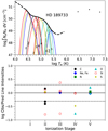 |
Fig. 1 Upper panel: emission measure distribution of HD 189733 calculated using the line fluxes measured in the HSLA/COSsummed spectrum. The 3-T model used to fit XMM-Newton summed EPIC spectra is also displayed. The thin lines represent the relative contribution function for each ion (the emissivity function multiplied by the EMD at each point), following same colour code as in lower panel. The small numbers indicate the ionisation stages of the species. Lower panel: observed-to-predicted line flux ratios for the ion stages in the upper panel. The dotted lines denote a factor of 2. |
3.2 Stellar fluxes
A further input parameter required by the model is the stellar XUV spectral flux. For HD 189733, a coronal model was used to obtain the stellar emission in the range of 5–1200 Å. The model is based on the addition of all the XMM-Newton observations available to date of this star, between 2007 and 20153. The EPIC spectra werecombined for a total exposure time of 461 ks (pn), 822 ks (MOS1), and 896 ks (MOS2). The coronal 3-Temperature model (log T(K) = 6.44 ± 0.01, 6.88 ± 0.01, 7.3 ± 0.01, log EM(cm−3) = 50.59 ± 0.03, 50.78 ± 0.04, 50.56 ± 0.01, LX = 2.2 × 1028 erg s−1) is complemented with line fluxes (Table A.1) from the HST/COS FUV spectrum available from the Hubble Spectral Legacy Archive (HSLA) to extend the model (Tables A.2 and A.3) towards lower temperatures (log T(K) ~ 4.0−5.9), following Sanz-Forcada et al. (2011). This model (Fig. 1) is a substantial improvement with respect to the X-exoplanets model available in Sanz-Forcada et al. (2011). The modelled spectral energy distribution (SED) fluxes now indicate an EUV luminosity of LEUV H = 1.6 × 1029 erg s−1 and LEUV He = 5.1 × 1028 erg s−1 in the ranges of 100–912 and 100-504 Å, respectively. The SED covers the range of 5–1145 Å, and it was generated following Sanz-Forcada et al. (2011). The data include several small flares, which were not removed on purpose, in order to provide an average model of active and non-active stages. We, therefore, used the summed HST/COS spectrum in the range of 1145–1450 Å. The SED calculated using our model is consistent with the flux level observed in the actual HST observations of the star in the region of 1145−1200 Å.
XMM-Newton observations of GJ 3470 were used to model the corona of this star, complemented with HST/STIS spectral line fluxes, as described in Bourrier et al. (2018). The quality of the HST/COS spectra was not good enough to fix the UV continuum in the spectral range of 1150–1750 Å, due to poor statistics, while HST/STIS coverage was limited to 1195–1248 Å only. Thus, the model SED was also used in this spectral range.
In order to extend the SED of both planets to 2600 Å, we used the stellar atmospheric model of Castelli & Kurucz (2004) scaled to the corresponding temperature, surface gravity, and metallicity (see Table 1). The composite SED for the spectral range of 5−2600 Å for both planets at their respective orbital separations are shown in Fig. 2.
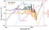 |
Fig. 2 Flux density (left y-axis) for HD 189733 (black) and GJ 3470 (orange) at 0.0332 and 0.0348 au plotted at a resolution of 10 Å, respectively. The H, He singlet, and He triplet ionisation cross sections (right y-axis) are also shown. |
3.3 Spectral absorption
With the He(23S) calculations and gas radial velocities from the model described above, we computed the He(23S) absorption by using a radiative transfer code for the primary transit geometry (Lampón et al. 2020). The spectroscopic data for the three metastable helium lines were taken from the NIST Atomic Spectra Database4. Doppler line shapes are assumed at the atmospheric temperature used in the model density, and an additional broadening produced by turbulent velocities can be included if necessary (vturb =  , where m is the mass of an He atom, see Eq. (16) in Lampón et al. 2020). The component of the radial velocity of the gas along the line of sight (LOS) towards the observer is also included in order to account for the motion of He(23S) as predicted in the hydrodynamic model. In addition to the radial velocities, averaged winds (e.g. day-to-night and super-rotation winds), and planetary rotation (see e.g. Salz et al. 2018; Seidel et al. 2020) can also be included in the radiative transfer model, as required (see Eq. (15) in Lampón et al. 2020).
In this study, we performed the integration of the He(23S) absorption up to 10 RP. This is motivated because we found that the He(23S) distribution of GJ 3470 b is rather extended (see Sect. 4.3).
3.4 Grid of simulations
Here we have analysed the mid-transit absorption profiles of HD 189733 b and GJ 3470 b (see Fig. 3) in a similar manner as in Lampón et al. (2020) for HD 209458 b. Briefly, from this model and the measured He(23S) absorption, we could not unambiguously determine the mass-loss rate and temperature of the planetary atmosphere as these two quantities are degenerate in most cases. Thus, for a given H/He composition, we ran the He(23S) model for a range of temperatures and mass-loss rates and computed the He(23S) absorption. As also shown by Lampón et al. (2020), the temperatures and mass-loss rates are also degenerate with respect to the H/He atomic ratio. We broke that degeneracy by also fitting the H0 density profiles of the model to those derived from Lyα measurements. To that end, we ran several sets of models for H/He atomic ratios ranging from 90/10, our nominal case, to 99.9/0.1 and to 99/1 for HD 189733 b and GJ 3470 b, respectively.
Synthetic spectra from these simulations were compared to the measured absorption profiles, and the corresponding reduced χ2 values were computed by (see, e.g. Press et al. 2007)
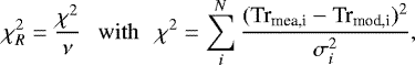
where ν = N − 2 is the number of degrees of freedom, N is the number of fitted spectral points, Trmea,i and Trmod,i are the measured and calculated transmissions, and σi is the error of the transmissions (see Fig. 3). For obtaining the uncertainties in the derived parameters T and Ṁ with this method, we considered the 95% confidence levels of the χ2 (not the reduced χ2). In addition, we also explored the posterior probability distribution of the three model parameters for the grid of model spectra discussed above by using the Markov chain Monte Carlo (MCMC) method (Sect. 4.5).
4 Results and discussion
4.1 He I transmission spectra
Our aim is to concentrate on the mid-transit absorption, which provides information about the main structure of the thermospheric escaping gas, but not to explain all the He(23S) absorption features of those planets, nor their variations along the transit. In particular, the analysis of the velocity shifts in the He(23S) absorption is potentially interesting because it would provide information about the 3D velocity distribution, its origin (e.g. day-to-night and super-rotation winds, and planet’s rotation), and it may also break some of the degeneracy between the temperature and mass-loss rates. However, as our model is spherically symmetric, it cannot explain net blue or red shifts and, hence, such analysis is beyond the scope of this paper. Nevertheless, in order to obtain the best fit to the mid-transit spectra, we need to assume some net velocities along the observational LOS superimposed on the gas radial velocities of our model. Thus, before exploring the range of temperature and mass-loss rates (see Sect. 4.2 and Figs. 4 and 5), we first discuss the shape of the mid-transit spectra and the required additional velocities.
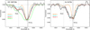 |
Fig. 3 Spectral transmission of the He triplet at mid-transit for HD 189733 b and GJ 3470 b (we note the different y-axis scale). Data points and their respective error bars are shown in black (adapted from Salz et al. 2018 and Pallé et al. 2020, respectively). Wavelengths are given in vacuum. The best-fit simulations are shown with red curves. For HD 189733 b, the best fit corresponds to a temperature of 10 000 K, a mass-loss rate of 109 g s−1 and an H/He mole-fraction of 90/10. For GJ 3470 b, the best fit corresponds to a temperature of 6000 K, Ṁ = 3.2 × 10¹⁰ g s−1 and an H/He of 90/10. Other models are described in Table 2. The positions of the helium lines are marked by vertical dotted (weak) and dot-dashed (strong) lines. |
4.1.1 He(23S) absorption of HD 189733 b
According to the observations by Salz et al. (2018), HD 189733 b shows a significant He excess absorption peaking at mid-transit (see Fig. 3), which is much stronger than that of HD 209458 b (see Alonso-Floriano et al. 2019; Lampón et al. 2020). The absorption profile also exhibits a more pronounced displacement to bluer wavelengths (− 3.5 ± 0.4 km s−1) and it is also significantly broader. A similar net blue shift has been observed in the He(23S) absorption of GJ 3470 b (see below and Pallé et al. 2020). Then, in order to obtain the best possible fit, we incorporated a net blue shift of −3.5 km s−1 in our simulations.
A further analysis of the spectrum shows that, at typical thermospheric temperatures for this planet, ~12 000 K (see, e.g. Guo 2011; Salz et al. 2016; Odert et al. 2020), the Doppler broadening is insufficient to explain the width of theabsorption profile (see Model A in left panel of Fig. 3). To achieve a similar width, we would need temperatures much higher than 20 000 K, which do not seem very realistic. Including a turbulence broadening component (see Sect. 3.3), the profile broadens, but it is still narrower than the measured absorption. In that calculation we also included the component of the gas radial velocities of our model along the observation LOS. However, since the absorption is confined to the first few thousands of kilometres and our velocities at these altitudes are rather slow (see left panels of Figs. 6 and 7), the induced broadening is negligible. Hence, our hydrodynamic model alone is not able to explain the width of the absorption profile.
A likely explanation of the broadening emerges from the inspection of the observed shifts of the absorption profile during the ingress and egress transit phases (Sect. 2, Salz et al. 2018). These shifts can be produced by a combination of the planetary rotation and strong net winds (probably of day-to-night and super-rotational winds) (see e.g. Salz et al. 2018; Flowers et al. 2019; Seidel et al. 2020), at altitudes ~1–2 RP, where the He(23S) absorption mainly takes place (see left panel of Fig. 6). In particular, Salz et al. (2018) derived an averaged wind in the range of −11.6 to −13.6 km s−1 from the blue shift in the egress, and an averaged wind in the range of 3.4 to 9.6 km s−1 from the red shift in the ingress. Thus, we fitted the absorption by including, in addition to the main atmospheric blue component at −3.5 km s−1, a blue and a red atmospheric component. By perturbing the velocity and fractional contribution of those components and minimising the χ2, we found that the absorption profile can be well reproduced by two components at −12 and 5 km s−1, covering about 25 and 28% of the disk, respectively (Models B and C in the left panel of Fig. 3). We note that those velocities are very similar to the mean values of the winds derived by Salz et al. (2018) from the egress and ingress phases. Also our red-shifted atmospheric fraction agrees very well, although the blue-shifted fraction is smaller in our case (mid-transit) than in the egress. These three components are included when we analyse the best fit to the spectra, for example in Model C (see Sect. 4.2).
Our model can also fit the absorption in the weaker He(23S) line (near 10 832 Å) (see Model C in left panel of Fig. 3). This is due to the assumption of a lower boundary with a high enough density so that it absorbs all the XUV flux reaching this altitude (compare Models C, with a boundary condition, and B, without a boundary condition, in that figure). As the strong stellar radiation reaches the lower boundary of the upper atmosphere of HD 189733 b (see left panel of Fig. 8), and since the stronger lines are saturated at low altitudes, the relative absorption of the stronger lines with respect to the weaker lines decreases.
However, in order to fit the He Iλ10833/He Iλ10832 ratio, we had to increase the lower boundary density up to 1018 cm−3, which agrees with the result of a very compressed annulus suggested by Salz et al. (2018). At this high concentration, collision processes become more important, increasing the production of He(23S) via recombination, because of the increase in He+ by charge-exchange, and by electron collision (see Table 2 in Lampón et al. 2020). These processes are more important at high temperatures (see inset in Fig. 6). Overall, the fitting of the He Iλ10833/He Iλ10832 ratio in this planet requires a very compressed and hot lower boundary.
It is worth noting that our model reproduces the measured He Iλ10833/He Iλ10832 ratio of 2.8 better than the simple annulus model of Salz et al. (2018), who obtained a value of 4.6. The key difference is that while the annulus is optically thick to the stronger lines in all its extension, 1.2 RP, they are only optically thick at the lower altitudes in our model.
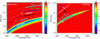 |
Fig. 4 Contour maps of the reduced χ2 of the He(23S) absorption for HD 189733 b (left panel) and GJ 3470 b (right panel) for an H/He ratio of 90/10. We note the different scales of temperatures and Ṁ. Dotted curves represent the best fits with filled circles denoting the constrained ranges for a confidence level of 95% (see Sect. 3.4). Over-plotted are also the curves and symbols for several H/He ratios, as labelled. The labels correspond to the hydrogen percentage, e.g. ‘90’ for an H/He of 90/10 and ‘95’ for H/He = 95/5 (see Sect. 4.4). The black dots represent the grid of the simulations. |
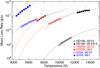 |
Fig. 5 Ranges of temperature and mass-loss rates for HD 209458 b, HD 189733 b, and GJ 3470 b for H/He ratios of 90/10 and 99.5/0.5, 90/10 and 98/2, as well as 90/10 and 99/1, respectively. Dotted lines show the ranges explored and symbols correspond to the constrained ranges (see Sect. 3.4). The values for HD 209458 b were taken from Lampón et al. (2020). The limited ranges (symbols) for this planet were obtained from heating efficiency considerations. |
4.1.2 Comparison with previous estimations of gas radial velocities of HD 189733 b
Seidel et al. (2020) have recently re-analysed observations of Na in HD 189733 b and have retrieved vertical upward winds, for example, radial velocity winds, of 40 ± 4 km s−1 at altitudes above 1 μbar. The region probed by them, however, is limited to below ~16 000 km (see their Fig. 8) (1.2 RP referred to the centre of the planet), that is, the 1 μbar to ~1 nbar or, approximately, (5–16) × 103 km or (1.06–1.2) RP region. They also suggest that such high radial velocities could arise from the expanding thermosphere. Our model velocities are much lower than 40 km s−1 (see Fig. 7, left panel); although, they could be affected by the imposed null velocity at the base of our model at 1.02 RP.
In order to verify if the shape of the measured He(23S) absorption profile is compatible with the value derived by Seidel et al., we simulated an absorption profile with the He(23S) densities derived in this work, but by assuming that the atmosphere is escaping at a constant radial velocity of 40 km s−1 at all altitudes. The He(23S) abundances that fit the absorption (see left panel of Fig. 6) have a very pronounced peak at the lower altitudes of our model, 1–1.5 RP. Hence, in essence, that is equivalent to imposing a constant 40 km s−1 velocity in that region. In order to be conservative, we did not include the turbulent component of the Doppler broadening in this calculation. The results show (see Fig. 3, Model D in green) that at such a high velocity, the He(23S) absorption profile would be much broader than measured. At those altitudes, (1.06–1.2) RP, the atmosphere is still dense enough to drag all atoms at a similar radial velocity (Murray-Clay et al. 2009). That is to say the velocities derived from either He or Na should not differ significantly. Hence, we conclude that such a high radial (vertical) velocity of 40 ± 4 km s−1 is not compatible with the He(23S) measurements, but this rather suggests that the gas radial velocities at those altitudes are significantly smaller.
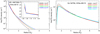 |
Fig. 6 He(23S) concentration profiles that best fit the measured absorption; i.e. for the white (HD 189733 b) and dark blue (GJ 3470 b) filled circles in Fig. 4. We note the different scale of the x-axis. The inset inthe left panel shows a zoom at low radii. |
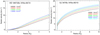 |
Fig. 7 Gas radial velocities of the model for the best fits of the He(23S) measured absorption; i.e. for the white (HD 189733 b) and dark blue (GJ 3470 b) filled circles in Fig. 4. We note the different scale of the x-axis. |
4.1.3 He(23S) absorption of GJ 3470 b
GJ 3470 b shows a significantly larger He excess absorption than HD 189733 b (we note the different y-axis scale in Fig. 3). Also, the absorption profile of the two stronger lines that are combined near 10 833 Å is broader. As for HD 189733 b, we have included the Doppler and turbulence broadening in the calculation. This warm Neptune has a weaker gravity thatleads to a much more extended atmosphere which expands at larger velocities (see right panels of Figs. 6 and 7). In fact, the velocities are already significant at rather low radii. Thus, in contrast to HD 189733 b, the component of the gas radial velocity along the observer LOS produces a significant broadening. We observe in Fig. 3 (right panel) that the models that include the radial velocities (Fand G), in contrast to E, explain very well the observed broadening without the need of blue or red components. We should also note that (not shown in the figure) the turbulent broadening is negligible compared to the broadening caused by such high radial velocities, and hence it does not have any significant impact on the line width.
As found in HD 189733 b (see above), as well as in HD 209458 b (Alonso-Floriano et al. 2019), we also observe a significant blue shift of the whole absorption, estimated to be −3.2 ± 1.3 km s−1 (Pallé et al. 2020). This is intermediate between the values measured in those two planets. Unfortunately, we do not have ingressor egress spectra with a sufficient S/N (as we did for HD 189733 b) to help us in understanding its origin. A likely explanation is that it is also produced by day-to-night winds with velocities along the LOS of −3.2 km s−1 (see model F in Fig. 3). However, as GJ 3470 b has a very extended atmosphere, with significant He(23S) absorption beyond the Roche lobe (see left panel of Fig. 6), another plausible interpretation is an upper atmosphere with no significant day-to-night winds below the Roche radius (3.6 RP, see Table 3) but with the unbound gas above the Roche lobe blue-shifted by processes, such as stellar wind interactions or stellar radiation pressure (see e.g. Salz et al. 2016). Model G (red curve in right panel of Fig. 3) shows the absorption of those simulations assuming that the gas above the Roche lobe is escaping at an LOS velocity of −5.0 km s−1. This scenario is consistent with that proposed by Bourrier et al. (2018) to explain the blue-shifted absorption signature of their Lyα observations.
The absorption of the weaker He(23S) line near 10 832 Å is also significantly broadened, and it is well reproduced within the estimated error bars. We note though that, in contrast to HD 189733 b, the stronger lines are not saturated at any radii and hence the ratio of the strong to the weaker lines is larger in this planet. Thus, the He(23S) absorption of this planet is rather insensitive to its lower boundary atmospheric conditions.
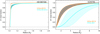 |
Fig. 8 H+ mole fraction profiles resulting from the fit of the measured absorption (filled circles in Fig. 4) for H/He = 90/10 and 99.5/0.5 for HD 189733 b (left panel) and 90/10 and 99/1 for GJ 3470 b (right panel). We note the different x-axis range. The solid thicker lines are the mean profiles. |
Planet parameters, the XUV flux, and EW(He(23S)) absorption.
4.2 Constraining the temperatures and mass-loss rates by the χ2 analysis
The T-Ṁ curves dictated by the He(23S) absorption of both planets show the typical behaviour of a positive correlation (see Fig. 4). That is to say for a given He(23S) concentration (imposed by the measured absorption profile), if temperature increases, the He(23S) concentration decreases and its maximum tends to move to lower altitudes (with smaller effective absorption areas) which, in order to be balanced, requires an increase in Ṁ.
Different H/He compositions of the thermospheric gas show different T–Ṁ curves, as was studied for HD 209458 b by Lampón et al. (2020). For a given mass-loss rate and temperature, the effect of increasing the H/He ratio results in a decrease in the global mass density, and the hydrogen and He(23S) concentrations, (see Fig. 13 of Lampón et al. 2020). Then, to compensate for the He(23S) absorption, the mass-loss rate has to be increased. In summary, for a fixed temperature, the higher the H/He ratio is, the higher the mass-loss rate required to reproduce the He(23S) absorption.
In comparing the results of HD 189733 b and GJ 3470 b (Fig. 4) with those of HD 209458 b (Fig. 8 of Lampón et al. 2020), we can appreciate that the T-Ṁ curves of HD 189733 b and GJ 3470 b are better constrained. In the case of HD 189733 b, the reduction of the degeneracy comes from the fitting of the He Iλ10833/He Iλ10832 ratio and from the temperature broadening, principally when including the turbulence.
The minima of  for HD 189733 b are larger at temperatures below ~10 000 K and above ~12 500 K. For lower temperatures, despite the high density in the lower boundary of this planet, He(23S) density is too low for fitting the weaker line, similar to Model B in Fig. 3; while at high temperatures, it is well fitted (see Sect. 4.1.1). At temperatures above ~12 500 K, the lines aretoo broadened, particularly when including the turbulence, and then the fitting is worse. It is interesting to look at the T/Ṁ constrain when neglecting the turbulence (see Fig. C.1). We see that the constrain changes significantly, leading in general to larger temperatures and mass-loss rates although the fit is not so good (larger minimum χ2).
As the strong line of HD 209458 b and GJ 3470 b is not saturated at any altitude, the He Iλ10833/He Iλ10832 ratio does not contribute to reduce the model degeneracy for these exoplanets. For GJ 3470 b, as the broadening of the gas radial velocities is very large, the effects of the turbulence are negligible.
In the case of GJ 3470 b, the reduction of the degeneracy comes from the large radial velocities (see right panel of Fig. 7). As we can see in Fig. 4 (right panel), χ2 is worse at temperatures below about 5400 K and higher than ~6900 K. At lower temperatures, the velocities are smaller and the broadening of the absorption profile narrower. The opposite occurs for higher temperatures. Thus, radial velocities calculated by the hydrodynamic model help to constrain the T-Ṁ curves of GJ 3470 b. However, HD 209458 b and HD 189733 b do not have such high radial velocities, so they do not help to reduce the degeneracy in these exoplanets.
We note that as the T-Ṁ degeneracy of HD 209458 b is not reduced by fitting the He Iλ10833/He Iλ10832 ratio nor by the gas radial velocities, Lampón et al. (2020) reduced it by applying constraints on the heating efficiencies. This criterion, however, cannot be used to reduce the degeneracy in HD 189733 b as heating efficiencies in this exoplanet are rather uncertain because of the significant radiative cooling (see, e.g. Salz et al. 2015, 2016).
We have found that the mass-loss rates of GJ 3470 b are much larger than those of HD 189733 b (Fig. 4); they are more than a factor of 10 for similar temperatures and an H/He ratio of 90/10. For larger H/He ratios, this difference decreases. Using the T-Ṁ curve of HD 209458 b as a reference (Lampón et al. 2020, reproduced in Fig. 5), we observe that the corresponding curves for HD 189733 b and GJ 3470 b are located in opposite regions, below and above that of HD 209458 b. On the one hand, the mass-loss rate of HD 189733 b is more than one order of magnitude smaller than that of HD 209458 b, and it is located at higher temperatures. The larger XUV flux of HD 189733 b (see Table 3) favours its larger temperatures. However, its larger gravity prevents its evaporation, resulting in much lower mass-loss rates. On the other hand, GJ 3470 b is not only irradiated in the XUV at higher levels than HD 209458 b (although only slightly), but it also has a much smaller gravity (see Table 3). Both factors favour its larger mass-loss rate, although the second is by far the most important. Those factors lead to a very extended atmosphere for GJ 3470 b and a rather compressed one for HD 189733 b (see Fig. 6); while the He(23S) concentration drops by a factor of 10 in ~7 RP for GJ 3470 b, it takes only ~0.5 RP for HD 189733 b. Likewise, the velocities of atmospheric expansion of GJ 3470 b are significantly larger than those of HD 189733 b (see Fig. 7). It is important to note that for GJ 3470 b, the velocities are already significant at very small radii, which, together with the large He(23S) abundances at these distances, contribute to a significant broadening of the absorption profile (see Sect. 4.1.3).
4.3 He(23S) density profiles and ionisation of the upper atmosphere
In this section we show the derived He(23S) densities, gas radial velocities, and the ionisation state of the upper atmospheres of HD 189733 b and GJ 3470 b. The He(23S) density profiles for our nominal case of H/He = 90/10 are shown in Fig. 6 (the profiles for the derived H/He ratios are shown in Fig. B.1). The densities of HD 189733 b peak at its lower boundary. GJ 3470 b shows more extended He(23S) density profiles with lower values at lower altitudes and larger values at higher altitudes. The peaks of the density profiles for this planet are also well confined to the range of 1.3–1.5 RP.
The results for the gas radial velocities are shown in Fig. 7 for the nominal H/He = 90/10, and in Fig. B.2 for the derived H/He ratios. GJ 3470 b is already expanding at large velocities at rather low altitudes, which is supported by the rather wide observed absorption profile. Figure 3 shows (right panel, Model E, orange) that if these radial velocities are not included, the He(23S) line profile would be significantly narrower.
The resulting ionisation fronts can be seen in the H+ mole fractions plotted in Fig. 8 for the nominal and the derived H/He ratios. The ionisation front of HD 189733 b is closer to theplanet’s lower boundary and narrower than that of GJ 3470 b. That is, for HD 189733 b, the stellar flux is strongly absorbed in a narrow altitude interval near the lower boundary, while in the case of GJ 3470 b, it is absorbed progressively in a wide range of altitudes at relatively large distances. Nonetheless, the effective absorption radius, RXUV, the distancewhere the optical depth for the XUV radiation is unity (Watson et al. 1981), is 1.02 RP (i.e. the lower boundary) for HD 189733 b and is in the range (1.02–1.12) RP for GJ 3470 b. As the planetary XUV cross section varies with R , the stellar radiation energy absorbed by GJ 3470 b increases due to the hydrodynamic atmospheric escape, while that of HD 189733 bremains constant.
4.4 Constraining the H/He composition by the χ2 analysis
As in Lampón et al. (2020), we constrained the H/He ratio by matching the H0 abundance profiles imposed by the He(23S) observations with those derived from Lyα absorption measurements. By constraining the H/He ratio, we also reduced the T-Ṁ degeneracy (see Fig. 4).
For HD 189733 b, we compared our H0 abundance profiles to those retrieved by Salz et al. (2016) and Odert et al. (2020) from Lyα absorption measurements. These authors analysed the observations of Lecavelier des Etangs et al. (2012) using a 1D hydrodynamic model and assuming substellar conditions to be representative of the whole planet. While Salz et al. (2016) report a good fit of the Lyα absorption, Odert et al. (2020) slightly overestimateit. We performed Lyα absorption calculations and found, in effect, that the profile of Salz et al. (2016) fit the observations of Lecavelier des Etangs et al. (2012) better. In addition we obtained that the errors in these measurements are well embraced by the H0 profile of Salz et al. (2016) when scaled by factors of 0.1 and 10 (see upper panels in Fig. 9).
From the analysis of χ2 (i.e. the profiles that fit the measured He(23S) within the minimum χ2 values, see Sect. 3.4), we found that the H0 model density profiles for H/He ratios of 90/10, 95/5, and even for 98/2 (see upper left panel of Fig. 9) are significantly lower than that of Salz et al. (2016), including their estimated uncertainties, at all altitudes. Also, for an H/He ratio of 99.9/0.1 and larger values, the H0 Lyα density profile is clearly overestimated (upper right panel in Fig. 9). This analysis suggests that an H/He composition of ~ 99.5/0.5 is more probable (upper middle panel in Fig. 9). It is worth mentioning that using the XUV flux from the X-exoplanets model by Sanz-Forcada et al. (2011), which is about a factor of 3 smaller than that used here, we obtained a good agreement with an H/He of 98/2. That is to say, including the effects of several small flares in the stellar model (see Sect. 3.2), we obtained a more ionised atmosphere and then a higher H/He.
In the case of GJ 3470 b, Salz et al. (2016) calculated the H0 density for this planet, but they could not verify it because of the lack of Lyα absorption measurements. More recently, however, Bourrier et al. (2018) measured the Lyα absorption and concluded that the Salz et al. (2016) model underestimates the H0 density. As for HD 189733 b, we also performed Lyα absorption calculations and found that the profile of Salz et al. (2016) actually fit the observations of Bourrier et al. (2018) rather well. Further, we found that the errors in those observations are covered by the H0 profile of Salz et al. (2016) when divided by  and multiplied by 10 (see lower panels in Fig. 9).
Our χ2 analysis for GJ 3470 b shows that the H0 density profiles obtained with H/He ratios of 90/10 and 95/5 are significantly lower than those of Salz et al. (2018) at all altitudes (bottom left panel in Fig. 9). They agree rather well, however, within the estimated uncertainties, for H/He ratios of 98/2 and 99/1 (bottom middle panel in Fig. 9). For H/He ratios larger than 99.5/0.5, most of the H0 density profiles that fit the He(23S) absorption fall outside the estimated uncertainties of the H0 Lyα profile and hence are rather unlikely (bottom right panel in Fig. 9).
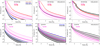 |
Fig. 9 Range of the neutral hydrogen concentration profiles (in grey shade areas) resulting from the fit of the measured absorption (filled circles in Fig. 4) for HD 189733 b (upper panels), GJ 3470 b (lower panels), and several H/He ratios, as labelled. The solid thicker curves are the mean profiles. The H0 density derived from Lyα measurements for HD 189733 b and GJ 3470 b by Salz et al. (2016) and our estimated uncertainties (× 10 and /10 for HD 189733 b, as well as ×10 and / |

4.5 MCMC analysis
In order to investigate the posterior probability distribution of model parameters for the described grid of models in Sect. 3.4, and to determine if the simultaneous MCMC fit constrains the parameters further by sampling the parameter-space effectively, we used a python implementation of emcee (Goodman & Weare 2010; Foreman-Mackey et al. 2013), called MCKM. The MCKM handles any arbitrary number of model parameters over regular (Cartesian) or irregularly spaced parameters, as well as any arbitrary number of data points and their respective covariance matrices.
We simultaneously fitted the observed He spectra and the H0 density derived from Lyα observations to constrain the temperatures, mass-loss rates, and H/He ratios of HD 189733 b and GJ 3470 b (see Fig. 10). We initialised 1000 walkers with uniform priors and with their range being the same as in the χ2 method to avoid differences between the two methods from different priors. Overall, the best models are consistent with the observations and no systematic residual is noticeable, except for the H0 density in the case of GJ 3470 b, where our models underestimate the density at low altitudes, R <2 RP. This could be due to the fact that we fitted global H0 density profiles (i.e. not at individual altitudes) and all of our modelled H0 profiles are systematically smaller than the profile of Salz et al. (2016) at R <2 RP. Further, because of the extended atmosphere of this planet, the atmospheric absorption at small radii is comparatively small and therefore has a weaker weight in the fitting of the whole atmosphere. Thus, both facts together could explain the underestimation.
Figure 11 shows the corner plot of the retrieved thermospheric parameters of HD 189733 b (red) and GJ 3470 b (blue). From this analysis, we find that the effective temperature, mass-loss rate, and H/He of HD 189733 b are T=12 400 K, Ṁ = (1.1 ± 0.1) × 1011 g s−1, and H/He = (99.2/0.8) ± 0.1, respectively. The retrieved values for GJ 3470 b are T = 6500
 K, Ṁ =
  ×1011 g s−1, and H/He = (97.1/2.9)
 .
.
4.6 Retrieved temperatures, mass-loss rates, and H/He composition
The results obtained by both the χ2 and the MCMC analysis are generally consistent. That is particularly clear in the case of HD 189733 b, for which the best fit of the H/He ratio derived from χ2 is very close to 99.5/0.5 and from the MCMC method we obtained H/He = (99.2/0.8) ± 0.1. The small uncertainty derived from the MCMC analysis is remarkable. Generally, one would expect a larger uncertainty range from the MCMC analysis than from the χ2 method, as the parameter space explored is wider. As explained above, a possible reason for the narrow MCMC posteriors might be that the MCMC fits the density profile at higher altitudes, but χ2 is fit at lower altitudes, particularly in the case of GJ 3470 b. The total number of data points at higher altitudes are more than that of the lower altitudes and hence a narrower posterior from such fit is not unexpected. The χ2 analysis suggests that they might be underestimated. Overall, as the most likely H/He ratio derived from both methods are very similar, we adopt the MCMC results of T = 12 400 K, that is, with an uncertainty of about 400 K; a mass-loss rate of Ṁ = (1.1 ± 0.1) × 1011 g s−1, which is very well constrained (see the almost flat T/Ṁ curves for high H/He ratios in left panel of Fig. 4), and an H/He = (99.2/0.8) ± 0.1, with possibly slightly larger uncertainties.
For GJ 3470 b, we have seen above that the MCMC analysis systematically underestimates the H0 density at low altitudes. This could be the reason of the significantly smaller derived H/He ratio by this method, H/He = (97.1/2.9) , than that suggested by the χ2 analysis of 99/1 (in the range of 98/2–99.5/0.5; bottom panels in Fig. 9). The general trend is to obtain larger H0 densities for larger H/He ratios. The H/He ratio has a rather important impact on the mass-loss rate of this planet, as well as on the temperature (see the rather steep T/Ṁ curves in the right panel of Fig. 4). Hence, the derived H/He has a significant impact on the resulting temperature and mass-loss rate ranges. Given the systematic underestimation of the H0 density by MCMC, we are more inclined to adopt the H/He values and uncertainties derived from the χ2 method, which also embraces the high probability peak value at H/He = 97 of MCMC (see Fig. 11). Thus, we conclude with a T = 5100 ± 900 K, an Ṁ = (1.9 ± 1.1) × 1011 g s−1, and an H/He = (98.5/1.5)
 for GJ 3470 b.
It is interesting to note that of the three exoplanets undergoing hydrodynamic escape which have been analysed thus from their He(23S) and Lyα observations (HD 209458 b by Lampón et al. 2020, and HD 189733 b and GJ 3470 b in this work), all show higher H/He ratios than the widely assumed 90/10, despite having rather different bulk parameters. Hence, this work suggests that an enrichment of H over He seems to be common in the upper atmospheres of giant exoplanets undergoing hydrodynamic escape.
One possibility to explain our results is that the escape of these atmospheres originates above the homopause, where, due to diffusive separation, the atmosphere is enriched in H over the heavier He atoms (see, e.g. Fig. 14 in Moses et al. 2005). Our results, however, could also be consistent with an origin of the escape near the homopause, at least for GJ 3470 b, as Hu et al. (2015) have shown that such enrichment is possible in Neptune and sub-Neptune exoplanets if the H mass-loss rate is comparable to its diffusion-limited mass-loss rate. This escape of H-enriched gas can lead, in the case of Neptune and sub-Neptunes, to an He and metal enrichment in the lower atmosphere with further consequences on their composition (e.g. abundances of carbon and oxygen-bearing species) (Hu et al. 2015; Malsky & Rogers 2020). Furthermore, according to these authors, it may even change the mass-radius relationship of the planet. In addition, our results are consistent with the depletion of atmospheric He by other processes as well, for example, with the formation of an H-He immiscibility layer in the interior of giant planets, as it produces He sequestration from the upper atmosphere (Salpeter 1973; Stevenson 1975, 1980; Wilson & Militzer 2010). This result also suggests that the H/He ratio might play a more important role than expected in the detectability of He(23S). In addition to the spectral shape and intensity of the XUV stellar irradiation (see, e.g. Oklopčić 2019), high H/He ratios could help to explain the non-detection of the He(23S) in some highly irradiated exoplanets, such as GJ 1214 b and GJ 9827 d (as suggested by Kasper et al. 2020) as well as K2-100b (Gaidos et al. 2020).
 |
Fig. 10 Bayesian inference of upper thermospheric conditions for HD 189733 b and GJ 3470 b. (a) Comparison of the best-fit model spectra (blue shaded area) and of the measured He triplet line for HD 189733 b (red data points). (b) Residualof the fitted models for HD 189733 b. The dotted horizontal lines mark 3-σ. (c) Comparison of the best-fit model H0 density (shaded blue area) and of the estimated H0 density from Lyα measurements for HD 189733 b (red data points). For the models, the blue area corresponds to the region of the posteriors between the 16 and 84% quantiles. d–f are similar to a–c, but for GJ 3470 b. |
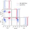 |
Fig. 11 Posterior probability distribution of our grid of models with respect to each of their parameter pairs as well as the marginalised distribution for each parameter for HD 189733 b (red) and GJ 3470 b (blue). The marginalised uncertainties are given as 16 to 84% quantiles. In the density maps, 1- and 2-σ are given as 1-e−0.5 ~0.393 and 1-e−2.0 ~0.865, respectively,as are common for multivariate MCMC results. |
5 Comparison of temperatures and mass-loss rates with previous works
5.1 HD 189733 b
Guilluy et al. (2020) observed the He(23S) absorption with the GIANO-B high-resolution spectrograph at the Telescopio Nazionale Galileo. They measured an He(23S) mid-transit absorption of 0.75 ± 0.03%, slightly lower than the 0.88 ± 0.04% by Salz et al. (2018); this was possibly due to the lower resolving power of GIANO-B with R ≈ 50 000 compared to CARMENES with R ≈ 80 400, as argued by Guilluy et al. (2020). These authors analysed their measurements with a 1D hydrodynamic isothermal Parker wind model (Parker 1958) for the thermosphere, and with a 3D particle model (Bourrier & Lecavelier des Etangs 2013) above 1.2 RP, the altitude where they estimated the gas becomes non-collisional. We applied a hydrodynamic model for the whole upper atmosphere because, as shown in our calculations, the altitude where the gas becomes non-collisional occurs far beyond the Roche lobe (in agreement with Salz et al. 2016; Odert et al. 2020). They estimated a T–Ṁ relationship that favoured a thermosphere with a T ≈12 000 K and an He(23S) density of 70 atoms cm−3 at 1.2 RP assuming solar-like H/He composition. Despite the different modelling and assumptions between the two analyses, our derived He(23S) distribution for the case of H/He = 90/10 and T = 12 000 K (see Fig. 6) agrees well with their He(23S) density at 1.2 RP. However, as we have shown in Sect. 4.6, our comparison with the Lyα measurements suggests an H/He composition of ~99.2/0.8, which leads to a higher mass-loss rate, Ṁ ≈10 × 1010 g s−1 (instead of Ṁ = 0.4 × 10¹⁰ g s−1 for H/He = 90/10), for T = 12 000 K (see Fig. 4).
Salz et al. (2016) simulated the upper atmosphere of HD 189733 b assuming that it is composed by ~90/10 of H/He, and using an incident FXUV ≈ 2.09 × 10⁴ erg cm−2 s−1. They used a comprehensive 1D hydrodynamic model and fitted the Lyα measurements of Lecavelier des Etangs et al. (2012). The resulting maximum temperature was 11 800 K and the mass-loss rate was Ṁ ≈1.7 × 10¹⁰ g s−1. For the same H/He composition, mass-loss rate, and maximum temperature, we overestimated the measured He(23S) absorption. Our results, Ṁ = (1.1 ± 0.1) × 1011 g s−1 and T = 12 400 K, show that our mass-loss rate range is larger by a factor of ~6.3 than that of Salz et al. (2016), while the maximum temperature is in good agreement. We note, however, that our stellar flux (see Table 3) is larger by a factor of 3 than that used by Salz et al. (2016), and our derived H/He composition is ≈99.2/0.8.
Odert et al. (2020) modelled the upper atmosphere of HD 189733 by also using a hydrodynamic approach for fitting the Lyα measurements of Lecavelier des Etangs et al. (2012). They assumed a thermosphere composed of H only and irradiated by FXUV ≈ 1.8 × 10⁴ erg cm−2 s−1. They obtained a maximum temperature of 11 000 K and a mass-loss rate of 5.4 × 10¹⁰ g s−1. We can see that our mass-loss rate range, Ṁ = (1.1 ± 0.1) × 1011 g s−1, is larger by a factor of ~2; our derived H/He composition is ≈ 99.2/0.8, which is close to the H-only composition assumed by Odert et al. (2020); and our temperature range, T = 12 400 K, is slightly larger than that obtained by Odert et al. (2020) Therefore, considering that our FXUV is larger by a factor of 3, our results are in good agreement with those of Odert et al. (2020)
Overall, we obtain similar mass-loss rates as Guilluy et al. (2020), when considering only the He(23S) absorption, but larger rates by a factor of ~25 when also considering the Lyα absorption. Salz et al. (2016) and Odert et al. (2020) derived mass-loss rates from Lyα measurements only. Our evaporation rates (constrained by both He(23S) and Lyα measurements) are larger (by a factor ~6.3) than those of Salz et al. (2016), who assumed an H/He composition of ~90/10; however, they are in good agreement (slightly larger by a factor of ~2) with those of Odert et al. (2020), who assumed an H-only atmosphere.
5.2 GJ 3470 b
Ninan et al. (2020) observed the He(23S) absorption with the Habitable Zone Planet Finder near-infrared spectrograph (HPF), on the 10 m Hobby-Eberly Telescope at the McDonald Observatory. They measured an equivalent width of the He(23S) mid-transit absorption of 0.012 ± 0.002 Å, which is lower than that calculated here of 0.0207 Å from the observations of Pallé et al. (2020). We note that differences could come from the different resolution power, as HPF has R ≈ 55 000, or from the different spectral integration interval (we include the absorption of the weak line, i.e. from 10 831.0 to 10 834.5 Å). They found that the model by Salz et al. (2016) overestimates their He(23S) measurements for this exoplanet, which agrees with our results.
Bourrier et al. (2018) modelled the upper atmosphere of GJ 3470 b with a parametrised thermosphere and a 3D particle model for non-collisional altitudes, assuming a thermospheric solar-like composition of H and He and a temperature of 7000 K. They fitted their Lyα observations obtaining an H0 mass-loss rate of ≈1.5 × 10¹⁰ g s−1. Our derived total (i.e. all neutral, ionised, and excited species) mass-loss rate is Ṁ = (1.9 ± 1.1) × 1011 g s−1, which agrees with the lower limit imposed by their H0 mass-loss rate.
Salz et al. (2016) modelled the upper atmosphere of GJ 3470 b with a comprehensive hydrodynamic model. For an H/He composition of ~90/10 and a FXUV ≈ 7.8 × 10³ erg cm−2 s−1, they estimated a Ṁ ≈ 1.9 × 10¹¹ g s−1 and a maximum thermospheric temperature of ≈8600 K. For the same H/He composition, mass-loss rate, and maximum temperature, we overestimated the He(23S) absorption, which agrees with Ninan et al. (2020). Our results, Ṁ = (1.9 ± 1.1) × 1011 g s−1, T = 5100 ± 900 K, and H/He = (98.5/1.5) , show that our mass-loss rates agree with those derived by Salz et al. (2016), although the temperature range is lower. We note, however, that our FXUV is about a factor of 2 lower (see Table 3).
Overall, by using the same solar H/He ratio, mass-loss rate, and temperature as Salz et al. (2016), we overestimated the He(23S) measurements of CARMENES, which agrees with the analysis of Ninan et al. (2020) from their HPF measurements. Our mass-loss rates, constrained by He(23S) and Lyα observations, agree with those of Salz et al. (2016), but for a higher H/He composition (98.5/1.5) . Also, our results agree with the lower limit of the mass-loss rate derived by Bourrier et al. (2018) from their Lyα measurements.
6 Summary
In this work we have studied the hydrodynamic atmospheric escape of the hot Jupiter HD 189733 b and the warm Neptune GJ 3470 b by analysing the mid-transit He(23S) absorption measurements observed with CARMENES (Salz et al. 2018; Pallé et al. 2020). We used a 1D hydrodynamic model with spherical symmetry (assuming substellar conditions apply to the whole planetary surface) and a non-LTE model for computing the population of He(23S). As a further constraint, we also used the neutral hydrogen density derived from Lyα measurements in previous studies.
The analysis of HD 189733 b shows that the lower boundary conditions are very important in explaining the anomalously large absorption in the weaker He(23S) line, which is caused by the hot and rather compressed upper atmosphere of this planet. It is worth mentioning that the absorption ratio of the weaker to stronger He(23S) lines helps in constraining the mass-loss rate and lower boundary conditions of its atmosphere. Thus, spectrographs with sufficient resolution for discriminating the weak and strong lines provide further information about the evaporating planets.
The radial velocities of our hydrodynamic model for HD 189733 b are too low to explain the broad absorption profile of this planet. In order to fit it, we need to incorporate blue-shifted components at −3.5 and –11.5 km s−1 covering nearly half and a quarter of the atmosphere’s terminator, respectively, as well as a red component at 5.5 km s−1 with 28% of the terminator coverage. We also found that a thermospheric constant radial velocity of 40 km s−1, as derived by Seidel et al. (2020), substantially overestimates the width of the He(23S) lines, suggesting that such a large velocity is unlikely.
In the case of GJ 3470 b, however, with a lower gravitational potential, our hydrodynamic model predicts gas radial velocities large enough to explain the width of the He(23S) absorption profile very well. This, in fact, helps in constraining its mass-loss rate and temperature. Furthermore, the measured absorption profile exhibits a net blue shift at −3.2 km s−1, which can be explained either by a net blue wind of the whole atmosphere at that velocity or by a combined atmosphere with a null blue shift below the Roche lobe and expanding at −5 km s−1 above.
These two planets have a similar He(23S) absorption, but rather different bulk parameters (see Table 3). In particular, the gravitational potential of HD 189733 b is near a factor of 10 larger and GJ 3470 b is irradiated in the XUV at about a factor of 14 smaller. In consequence, the characteristics of their upper atmospheres also differ significantly. Thus, while HD 189733 b has a rather compressed and warm atmosphere (12 400 K) with small gas radial velocities, GJ 3470 b exhibits a very extended and cooler (5100 ± 900 K) atmosphere with large radial velocities. Also, while the upper atmosphere of HD 189733 b is almost fully ionised beyond ≈1.1RP, GJ 3470 b exhibits a very wide ionisation front (from ~1.25 RP to far beyond its Roche lobe). Overall, the gravitational potential and the irradiation balance result in comparable mass-loss rates, Ṁ = (1.1 ± 0.1) × 1011 g s−1 versus Ṁ = (1.9 ± 1.1) × 1011 g s−1 for HD 189733 b and GJ 3470 b, respectively. The very different characteristics of these objects make them very suitable archetypes for benchmark studies on atmospheric loss.
We have further found that both planets have upper atmospheres with very low mean molecular masses (H/He = 97/3–99.5/0.5). It is remarkable that the three exoplanets with evaporating atmospheres that have been studied so far by using both He(23S) and Lyα observations (HD 209458 b, HD 189733 b, and GJ 3470 b) all show higher H/He ratios than the commonly assumed 90/10, despite having very different bulk parameters. This H-enrichment of the upper atmospheres could be explained, on the one hand, by the escape originating above the homopause, where the atmosphere is expected to be depleted in He by diffusive separation. Another possibility, particularly in the case of the warm Neptune GJ 3470 b, is that the escape originates from deeper altitudes, around the homopause, according to the prediction of Hu et al. (2015) of an H-enriched upper atmosphere for Neptune and sub-Neptunes undergoing hydrodynamic escape. They further predict that it could lead to an He-enrichment of the lower atmosphere, with important consequences on their atmospheric composition (abundances of carbon and oxygen-bearing species) and even on their mass-radius relationship. Our results also suggest that the H/He ratio might play a more important role than expected in the detectability of He(23S). The confirmation of this important result definitely calls for the study of other escaping atmospheres with concomitant He(23S) and Lyα measurements and for performing an independent analysis.
Here, we have analysed the He(23S) mid-transit absorption spectra of HD 189733 b and GJ 3470 b with a 1D spherical model. However, comprehensive multi-fluid magneto-hydrodynamic 3D models are needed to provide more detailed information about the spatial and velocity distribution of the gas, the origin of the non-radial winds, and the influence of other processes (e.g. stellar wind, radiation pressure, or magnetic field interactions). In particular, the analysis of the ingress and egress spectra of these planets would be very valuable.
Acknowledgements
We thank the referee for very useful comments. CARMENES is an instrument for the Centro Astronómico Hispano-Alemán (CAHA) at Calar Alto (Almería, Spain), operated jointly by the Junta de Andalucía and the Instituto de Astrofísica de Andalucía (CSIC). CARMENES was funded by the Max-Planck-Gesellschaft (MPG), the Consejo Superior de Investigaciones Científicas (CSIC), the Ministerio de Economía y Competitividad (MINECO) and the European Regional Development Fund (ERDF) through projects FICTS-2011-02, ICTS-2017-07-CAHA-4, and CAHA16-CE-3978, and the members of the CARMENES Consortium (Max-Planck-Institut für Astronomie, Instituto de Astrofísica de Andalucía, Landessternwarte Königstuhl, Institut de Ciències de l’Espai, Institut für Astrophysik Göttingen, Universidad Complutense de Madrid, Thüringer Landessternwarte Tautenburg, Instituto de Astrofísica de Canarias, Hamburger Sternwarte, Centro de Astrobiología and Centro Astronómico Hispano-Alemán), with additional contributions by the MINECO, the Deutsche Forschungsgemeinschaft through the Major Research Instrumentation Programme and Research Unit FOR2544 “Blue Planets around Red Stars”, the Klaus Tschira Stiftung, the states of Baden-Württemberg and Niedersachsen, and by the Junta de Andalucía. We acknowledge financial support from the Agencia Estatal de Investigación of the Ministerio de Ciencia, Innovación y Universidades and the ERDF through projects ESP2016–76076–R, ESP2017–87143–R, PID2019-110689RB-I00/AEI/10.13039/501100011033, BES–2015–074542, PGC2018-099425–B–I00, PID2019-109522GB-C51/2/3/4, PGC2018-098153-B-C33, AYA2016-79425-C3-1/2/3-P, ESP2016-80435-C2-1-R, and the Centre of Excellence “Severo Ochoa” and “María de Maeztu” awards to the Instituto de Astrofísica de Canarias (SEV-2015-0548), Instituto de Astrofísica de Andalucía (SEV-2017-0709), and Centro de Astrobiología (MDM-2017-0737), and the Generalitat de Catalunya/CERCA programme. T.H. acknowledges support from the European Research Council under the Horizon 2020 Framework Program via the ERC Advanced Grant Origins 832428. A.S.L. acknowledges funding from the European Research Council under the European Union’s Horizon 2020 research and innovation program under grant agreement No 694513.
Appendix A Data for calculating the stellar flux of HD 189733
Data used in the modelling of the stellar flux of HD 189733 in Sect. 3.2. The spectrum was downloaded from the Hubble Spectral Legacy Archive (HSLA); a sum of 42 HD 189733 spectra were acquired with the COS/G130M grating. The exposures were taken in 2009, 2013, and 2017 (proposals IDs 11673, 12984, and 14767).
HST/COS line fluxes of HD 189733.
Emission measure distribution of HD 189733.
Transition region abundances of HD 189733 (solar units).
Appendix B Results for the derived H/He compositions
He(23S) density profiles and gas radial velocities for the derived H/He ratios of HD 189733 b and GJ 3470 b.
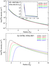 |
Fig. B.1 He(23S) concentration profiles that best fit the measured absorption (i.e. the filled circles in Fig. 4) for HD 189733 b and an H/He ratio of 99.5/0.5 (upper panel), as well as for GJ 3470 b and H/He = 99/1 (lower panel). |
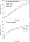 |
Fig. B.2 Gasradial velocities of the hydrodynamic model for the best fit of the measured absorption (i.e. the filled circles in Fig. 4) for HD 189733 b and an H/He ratio of 99.5/0.5 (upper panel), as well as for GJ 3470 b and H/He = 99/1 (lower panel). |
Appendix C Results for neglecting the broadening turbulence
Results forthe T-Ṁ map for HD 189733 b when the turbulence broadening is not considered.
 |
Fig. C.1 Contour maps of the reduced χ2 of the model of the helium triplet absorption for HD 189733 b for several H/He ratios (as in Fig. 4, left panel) whenthe turbulence broadening is not considered. The filled circles highlight the best fits (constrained ranges). The black dots represent the grid of the models. |
References
- Agol, E., Cowan, N. B., Knutson, H. A., et al. 2010, ApJ, 721, 1861 [NASA ADS] [CrossRef] [Google Scholar]
- Allart, R., Bourrier, V., Lovis, C., et al. 2018, Science, 362, 1384 [Google Scholar]
- Allart, R., Bourrier, V., Lovis, C., et al. 2019, A&A, 623, A58 [NASA ADS] [CrossRef] [EDP Sciences] [Google Scholar]
- Alonso-Floriano, F. J., Snellen, I. A. G., Czesla, S., et al. 2019, A&A, 629, A110 [NASA ADS] [CrossRef] [EDP Sciences] [Google Scholar]
- Anders, E., & Grevesse, N. 1989, Geochim. Cosmochim. Acta, 53, 197 [Google Scholar]
- Asplund, M., Grevesse, N., Sauval, A. J., & Scott, P. 2009, ARA&A, 47, 481 [NASA ADS] [CrossRef] [Google Scholar]
- Baluev, R. V., Sokov, E. N., Shaidulin, V. S., et al. 2015, MNRAS, 450, 3101 [NASA ADS] [CrossRef] [Google Scholar]
- Baraffe, I., Selsis, F., Chabrier, G., et al. 2004, A&A, 419, L13 [NASA ADS] [CrossRef] [EDP Sciences] [Google Scholar]
- Baraffe, I., Chabrier, G., Barman, T. S., et al. 2005, A&A, 436, L47 [NASA ADS] [CrossRef] [EDP Sciences] [Google Scholar]
- Ben-Jaffel, L., & Ballester, G. E. 2013, A&A, 553, A52 [NASA ADS] [CrossRef] [EDP Sciences] [Google Scholar]
- Bonfils, X., Gillon, M., Udry, S., et al. 2012, A&A, 546, A27 [NASA ADS] [CrossRef] [EDP Sciences] [Google Scholar]
- Bouchy, F., Udry, S., Mayor, M., et al. 2005, A&A, 444, L15 [EDP Sciences] [Google Scholar]
- Bourrier, V., & Lecavelier des Etangs A. 2013, A&A, 557, A124 [NASA ADS] [CrossRef] [EDP Sciences] [Google Scholar]
- Bourrier, V., Lecavelier des Etangs, A., Dupuy, H., et al. 2013, A&A, 551, A63 [NASA ADS] [CrossRef] [EDP Sciences] [Google Scholar]
- Bourrier, V., Lecavelier des Etangs, A., Ehrenreich, D., et al. 2018, A&A, 620, A147 [NASA ADS] [CrossRef] [EDP Sciences] [Google Scholar]
- Boyajian, T., von Braun, K., Feiden, G. A., et al. 2015, MNRAS, 447, 846 [NASA ADS] [CrossRef] [Google Scholar]
- Casasayas-Barris, N., Pallé, E., Yan, F., et al. 2018, A&A, 616, A151 [NASA ADS] [CrossRef] [EDP Sciences] [Google Scholar]
- Castelli, F., & Kurucz, R. 2004, IAU Symp. 210, A20 [Google Scholar]
- de Kok, R. J., Brogi, M., Snellen, I. A. G., et al. 2013, A&A, 554, A82 [NASA ADS] [CrossRef] [EDP Sciences] [Google Scholar]
- Eggleton, P. P. 1983, ApJ, 268, 368 [NASA ADS] [CrossRef] [Google Scholar]
- Ehrenreich, D., Lecavelier des Etangs, A., Hébrard, G., et al. 2008, A&A, 483, 933 [NASA ADS] [CrossRef] [EDP Sciences] [Google Scholar]
- Flowers, E., Brogi, M., Rauscher, E., Kempton, E. M.-R., & Chiavassa, A. 2019, ApJ, 157, 209 [Google Scholar]
- Foreman-Mackey, D., Hogg, D. W., Lang, D., & Goodman, J. 2013, PASP, 125, 306 [Google Scholar]
- Gaia Collaboration (Brown, A. G. A., et al.) 2018, A&A, 616, A1 [NASA ADS] [CrossRef] [EDP Sciences] [Google Scholar]
- Gaidos, E., Hirano, T., Mann, A. W., et al. 2020, MNRAS, 495, 650 [Google Scholar]
- García-Muñoz, A. 2007, Planet. Space Sci., 55, 1426 [NASA ADS] [CrossRef] [Google Scholar]
- Goodman, J., & Weare, J. 2010, Commun. Appl. Math. Comput. Sci., 5, 65 [Google Scholar]
- Guilluy, G., Andretta, V., Borsa, F., et al. 2020, A&A, 639, A49 [EDP Sciences] [Google Scholar]
- Guo, J. H. 2011, ApJ, 733, 98 [NASA ADS] [CrossRef] [Google Scholar]
- Hu, R., Seager, S., & Yung, Y. L. 2015, ApJ, 807, 8 [NASA ADS] [CrossRef] [Google Scholar]
- Kasper, D., Bean, J. L., Oklopčić, A., et al. 2020, ApJ, 160, 258 [Google Scholar]
- Koskinen, T., Harris, M., Yelle, R., & Lavvas, P. 2013, Icarus, 226, 1678 [Google Scholar]
- Lampón, M., López-Puertas, M., Lara, L. M., et al. 2020, A&A, 636, A13 [CrossRef] [EDP Sciences] [Google Scholar]
- Lecavelier des Etangs, A., Ehrenreich, D., Vidal-Madjar, A., et al. 2010, A&A, 514, A72 [NASA ADS] [CrossRef] [EDP Sciences] [Google Scholar]
- Lecavelier des Etangs, A., Bourrier, V., Wheatley, P. J., et al. 2012, A&A, 543, L4 [NASA ADS] [CrossRef] [EDP Sciences] [Google Scholar]
- Lopez, E. D., & Fortney, J. J. 2013, ApJ, 776, 2 [Google Scholar]
- Malsky, I., & Rogers, L. A. 2020, ApJ, 896, 48 [Google Scholar]
- Mansfield, M., Bean, J. L., Oklopčić, A., et al. 2018, ApJ, 868, L34 [Google Scholar]
- Moses, J. I., Fouchet, T., Bezard, B., et al. 2005, J. Geophys. Res., 110, E08001 [Google Scholar]
- Muñoz, A. G., & Schneider, P. C. 2019, ApJ, 884, L43 [CrossRef] [Google Scholar]
- Murray-Clay, R. A., Chiang, E. I., & Murray, N. 2009, ApJ, 693, 23 [Google Scholar]
- Ninan, J. P., Stefansson, G., Mahadevan, S., et al. 2020, ApJ, 894, 97 [Google Scholar]
- Nortmann, L., Palle, E., Salz, M., et al. 2018, Science, 362, 1388 [NASA ADS] [CrossRef] [EDP Sciences] [Google Scholar]
- Odert, P., Erkaev, N. V., Kislyakova, K. G., et al. 2020, A&A, 638, A49 [EDP Sciences] [Google Scholar]
- Oklopčić, A. 2019, ApJ, 881, 133 [Google Scholar]
- Oklopčić, A., & Hirata, C. M. 2018, ApJ, 855, L11 [Google Scholar]
- Owen, J. E., & Wu, Y. 2013, ApJ, 775, 105 [Google Scholar]
- Owen, J. E., & Wu, Y. 2017, ApJ, 847, 29 [Google Scholar]
- Pallé, E., Nortmann, L., Casasayas-Barris, N., et al. 2020, A&A, 638, A61 [EDP Sciences] [Google Scholar]
- Parker, E. N. 1958, ApJ, 128, 664 [Google Scholar]
- Poppenhaeger, K., Schmitt, J. H. M. M., & Wolk, S. J. 2013, ApJ, 773, 62 [NASA ADS] [CrossRef] [Google Scholar]
- Press, W. H., Teukolsky, S. A., Vetterling, W. T., & Flannery, B. P. 2007, Numerical Recipes 3rd Edition: The Art of Scientific Computing, 3rd edn. (Cambridge: Cambridge University Press) [Google Scholar]
- Quirrenbach, A., Amado, P. J., Caballero, J. A., et al. 2016, SPIE Proc., 12 [Google Scholar]
- Quirrenbach, A., Amado, P. J., Ribas, I., et al. 2018, SPIE Proc., 32 [Google Scholar]
- Salpeter, E. E. 1973, ApJ, 181, L83 [NASA ADS] [CrossRef] [Google Scholar]
- Salz, M., Schneider, P. C., Czesla, S., & Schmitt, J. H. M. M. 2015, A&A, 585, L2 [Google Scholar]
- Salz, M., Czesla, S., Schneider, P. C., & Schmitt, J. H. M. M. 2016, A&A, 586, A75 [NASA ADS] [CrossRef] [EDP Sciences] [Google Scholar]
- Salz, M., Czesla, S., Schneider, P. C., et al. 2018, A&A, 620, A97 [NASA ADS] [CrossRef] [EDP Sciences] [Google Scholar]
- Sanz-Forcada, J., Maggio, A., & Micela, G. 2003, A&A, 408, 1087 [NASA ADS] [CrossRef] [EDP Sciences] [Google Scholar]
- Sanz-Forcada, J., Micela, G., Ribas, I., et al. 2011, A&A, 532, A6 [NASA ADS] [CrossRef] [EDP Sciences] [Google Scholar]
- Seidel, J. V., Ehrenreich, D., Pino, L., et al. 2020, A&A, 633, A86 [NASA ADS] [CrossRef] [EDP Sciences] [Google Scholar]
- Spake, J. J., Sing, D. K., Evans, T. M., et al. 2018, Nature, 557, 68 [Google Scholar]
- Stevenson, D. J. 1975, Phys. Rev. B, 12, 3999 [NASA ADS] [CrossRef] [Google Scholar]
- Stevenson, D. J. 1980, Science, 208, 746 [NASA ADS] [CrossRef] [PubMed] [Google Scholar]
- Stone, J. M., & Proga, D. 2009, ApJ, 694, 205 [NASA ADS] [CrossRef] [Google Scholar]
- Tian, F., Toon, O. B., Pavlov, A. A., & De Sterck H. 2005, ApJ, 621, 1049 [NASA ADS] [CrossRef] [Google Scholar]
- Torres, G., Winn, J. N., & Holman, M. J. 2008, ApJ 2008, 677 [Google Scholar]
- Tripathi, A., Kratter, K. M., Murray-Clay, R. A., & Krumholz, M. R. 2015, ApJ, 808, 173 [Google Scholar]
- Vidal-Madjar, A., des Etangs, A. L., Désert, J.-M., et al. 2003, Nature, 422, 143 [NASA ADS] [CrossRef] [PubMed] [Google Scholar]
- Vidal-Madjar, A., Désert, J.-M., des Etangs, A. L., et al. 2004, ApJ, 604, 69 [Google Scholar]
- Watson, A. J., Donahue, T. M., & Walker, J. C. 1981, Icarus, 48, 150 [NASA ADS] [CrossRef] [Google Scholar]
- Wilson, H. F.,& Militzer, B. 2010, Phys. Rev. Lett., 104, 121101 [Google Scholar]
- Wyttenbach, A., Mollière, P., Ehrenreich, D., et al. 2020, A&A, 638, A87 [EDP Sciences] [Google Scholar]
- Yan, F., & Henning, T. 2018, Nat. Astron., 2, 714 [NASA ADS] [CrossRef] [Google Scholar]
- Yelle, R. V. 2004, Icarus, 170, 167 [Google Scholar]
At wavelengths 10 832.06, 10 833.22, and 10 833.31 Å in the vacuum, often referred to as their air wavelengths of 10 830 Å.
Calar Alto high-Resolution search for M dwarfs with Exoearths with Near-infrared and optical Échelle Spectrographs, at the 3.5 m Calar Alto Telescope.
Proposals id. 50607, 60097, 67239, 69089, 69229, 74498, 74839.
All Tables
All Figures
|
Fig. 1 Upper panel: emission measure distribution of HD 189733 calculated using the line fluxes measured in the HSLA/COSsummed spectrum. The 3-T model used to fit XMM-Newton summed EPIC spectra is also displayed. The thin lines represent the relative contribution function for each ion (the emissivity function multiplied by the EMD at each point), following same colour code as in lower panel. The small numbers indicate the ionisation stages of the species. Lower panel: observed-to-predicted line flux ratios for the ion stages in the upper panel. The dotted lines denote a factor of 2. |
| In the text | |
|
Fig. 2 Flux density (left y-axis) for HD 189733 (black) and GJ 3470 (orange) at 0.0332 and 0.0348 au plotted at a resolution of 10 Å, respectively. The H, He singlet, and He triplet ionisation cross sections (right y-axis) are also shown. |
| In the text | |
|
Fig. 3 Spectral transmission of the He triplet at mid-transit for HD 189733 b and GJ 3470 b (we note the different y-axis scale). Data points and their respective error bars are shown in black (adapted from Salz et al. 2018 and Pallé et al. 2020, respectively). Wavelengths are given in vacuum. The best-fit simulations are shown with red curves. For HD 189733 b, the best fit corresponds to a temperature of 10 000 K, a mass-loss rate of 109 g s−1 and an H/He mole-fraction of 90/10. For GJ 3470 b, the best fit corresponds to a temperature of 6000 K, Ṁ = 3.2 × 10¹⁰ g s−1 and an H/He of 90/10. Other models are described in Table 2. The positions of the helium lines are marked by vertical dotted (weak) and dot-dashed (strong) lines. |
| In the text | |
|
Fig. 4 Contour maps of the reduced χ2 of the He(23S) absorption for HD 189733 b (left panel) and GJ 3470 b (right panel) for an H/He ratio of 90/10. We note the different scales of temperatures and Ṁ. Dotted curves represent the best fits with filled circles denoting the constrained ranges for a confidence level of 95% (see Sect. 3.4). Over-plotted are also the curves and symbols for several H/He ratios, as labelled. The labels correspond to the hydrogen percentage, e.g. ‘90’ for an H/He of 90/10 and ‘95’ for H/He = 95/5 (see Sect. 4.4). The black dots represent the grid of the simulations. |
| In the text | |
|
Fig. 5 Ranges of temperature and mass-loss rates for HD 209458 b, HD 189733 b, and GJ 3470 b for H/He ratios of 90/10 and 99.5/0.5, 90/10 and 98/2, as well as 90/10 and 99/1, respectively. Dotted lines show the ranges explored and symbols correspond to the constrained ranges (see Sect. 3.4). The values for HD 209458 b were taken from Lampón et al. (2020). The limited ranges (symbols) for this planet were obtained from heating efficiency considerations. |
| In the text | |
|
Fig. 6 He(23S) concentration profiles that best fit the measured absorption; i.e. for the white (HD 189733 b) and dark blue (GJ 3470 b) filled circles in Fig. 4. We note the different scale of the x-axis. The inset inthe left panel shows a zoom at low radii. |
| In the text | |
|
Fig. 7 Gas radial velocities of the model for the best fits of the He(23S) measured absorption; i.e. for the white (HD 189733 b) and dark blue (GJ 3470 b) filled circles in Fig. 4. We note the different scale of the x-axis. |
| In the text | |
|
Fig. 8 H+ mole fraction profiles resulting from the fit of the measured absorption (filled circles in Fig. 4) for H/He = 90/10 and 99.5/0.5 for HD 189733 b (left panel) and 90/10 and 99/1 for GJ 3470 b (right panel). We note the different x-axis range. The solid thicker lines are the mean profiles. |
| In the text | |
|
Fig. 9 Range of the neutral hydrogen concentration profiles (in grey shade areas) resulting from the fit of the measured absorption (filled circles in Fig. 4) for HD 189733 b (upper panels), GJ 3470 b (lower panels), and several H/He ratios, as labelled. The solid thicker curves are the mean profiles. The H0 density derived from Lyα measurements for HD 189733 b and GJ 3470 b by Salz et al. (2016) and our estimated uncertainties (× 10 and /10 for HD 189733 b, as well as ×10 and / |
| In the text | |
|
Fig. 10 Bayesian inference of upper thermospheric conditions for HD 189733 b and GJ 3470 b. (a) Comparison of the best-fit model spectra (blue shaded area) and of the measured He triplet line for HD 189733 b (red data points). (b) Residualof the fitted models for HD 189733 b. The dotted horizontal lines mark 3-σ. (c) Comparison of the best-fit model H0 density (shaded blue area) and of the estimated H0 density from Lyα measurements for HD 189733 b (red data points). For the models, the blue area corresponds to the region of the posteriors between the 16 and 84% quantiles. d–f are similar to a–c, but for GJ 3470 b. |
| In the text | |
|
Fig. 11 Posterior probability distribution of our grid of models with respect to each of their parameter pairs as well as the marginalised distribution for each parameter for HD 189733 b (red) and GJ 3470 b (blue). The marginalised uncertainties are given as 16 to 84% quantiles. In the density maps, 1- and 2-σ are given as 1-e−0.5 ~0.393 and 1-e−2.0 ~0.865, respectively,as are common for multivariate MCMC results. |
| In the text | |
|
Fig. B.1 He(23S) concentration profiles that best fit the measured absorption (i.e. the filled circles in Fig. 4) for HD 189733 b and an H/He ratio of 99.5/0.5 (upper panel), as well as for GJ 3470 b and H/He = 99/1 (lower panel). |
| In the text | |
|
Fig. B.2 Gasradial velocities of the hydrodynamic model for the best fit of the measured absorption (i.e. the filled circles in Fig. 4) for HD 189733 b and an H/He ratio of 99.5/0.5 (upper panel), as well as for GJ 3470 b and H/He = 99/1 (lower panel). |
| In the text | |
|
Fig. C.1 Contour maps of the reduced χ2 of the model of the helium triplet absorption for HD 189733 b for several H/He ratios (as in Fig. 4, left panel) whenthe turbulence broadening is not considered. The filled circles highlight the best fits (constrained ranges). The black dots represent the grid of the models. |
| In the text | |
Current usage metrics show cumulative count of Article Views (full-text article views including HTML views, PDF and ePub downloads, according to the available data) and Abstracts Views on Vision4Press platform.
Data correspond to usage on the plateform after 2015. The current usage metrics is available 48-96 hours after online publication and is updated daily on week days.
Initial download of the metrics may take a while.