| Issue |
A&A
Volume 647, March 2021
|
|
|---|---|---|
| Article Number | A51 | |
| Number of page(s) | 14 | |
| Section | Cosmology (including clusters of galaxies) | |
| DOI | https://doi.org/10.1051/0004-6361/202039208 | |
| Published online | 08 March 2021 | |
Radio halos in a mass-selected sample of 75 galaxy clusters
II. Statistical analysis
1
Hamburger Sternwarte, Universität Hamburg, Gojenbergsweg 112, 21029 Hamburg, Germany
e-mail: This email address is being protected from spambots. You need JavaScript enabled to view it.
2
INAF-Istituto di Radioastronomia, via P. Gobetti 101, 40129 Bologna, Italy
3
Dipartimento di Fisica e Astronomia, Università di Bologna, via P. Gobetti 93/2, 40129 Bologna, Italy
4
Leiden Observatory, Leiden University, PO Box 9513, 2300 RA Leiden, The Netherlands
5
National Centre for Radio Astrophysics, Tata Institute of Fundamental Research Savitribai Phule Pune University Campus, Pune, 411 007 Maharashtra, India
6
AIM, CEA, CNRS, Université Paris-Saclay, Université Paris Diderot, Sorbonne Paris Cité, 91191 Gif-sur-Yvette, France
7
INAF, Osservatorio di Astrofisica e Scienza dello Spazio, via Pietro Gobetti 93/3, 40129 Bologna, Italy
8
INFN, Sezione di Bologna, viale Berti Pichat 6/2, 40127 Bologna, Italy
9
Naval Research Laboratory, 4555 Overlook Avenue SW, Code 7213, Washington, DC 20375, USA
Received:
18
August
2020
Accepted:
5
January
2021
Abstract
Context. Many galaxy clusters host megaparsec-scale diffuse radio sources called radio halos. Their origin is tightly connected to the processes that lead to the formation of clusters themselves. In order to reveal this connection, statistical studies of the radio properties of clusters combined with their thermal properties are necessary. For this purpose, we selected a sample of galaxy clusters with M500 ≥ 6 × 10¹⁴ M⊙ and z = 0.08 − 0.33 from the Planck Sunyaev–Zel’dovich catalogue. In Paper I, we presented the radio and X-ray data analysis that we carried out on the clusters of this sample.
Aims. In this paper we exploit the wealth of data presented in Paper I to study the radio properties of the sample, in connection to the mass and dynamical state of clusters.
Methods. We used the dynamical information derived from the X-ray data to assess the role of mergers in the origin of radio halos. We studied the distribution of clusters in the radio power–mass diagram, the scaling between the radio luminosity of radio halos and the mass of the host clusters, and the role of dynamics in the radio luminosity and emissivity of radio halos. We measured the occurrence of radio halos as a function of the cluster mass and we compared it with the expectations of models developed in the framework of turbulent acceleration.
Results. We find that more than the 90% of radio halos are in merging clusters and that their radio power correlates with the mass of the host clusters. The correlation shows a large dispersion. Interestingly, we show that cluster dynamics contributes significantly to this dispersion, with more disturbed clusters being more radio luminous. Clusters without radio halos are generally relaxed, and the upper limits to their diffuse emission lie below the correlation. Moreover, we show that the radio emissivity of clusters exhibits an apparent bimodality, with the emissivity of radio halos being at least ∼5 times larger than the non-emission associated with more relaxed clusters. We find that the fraction of radio halos drops from ∼70% in high-mass clusters to ∼35% in the lower mass systems in the sample and we show that this result is in good agreement with the expectations from turbulent re-acceleration models.
Key words: galaxies: clusters: general / galaxies: clusters: intracluster medium / radiation mechanisms: non-thermal
© ESO 2021
1. Introduction
An increasing number of galaxy clusters show diffuse synchrotron emission detected in the radio band. This emission reveals that the intracluster medium (ICM) is permeated with relativistic particles and magnetic fields. Cluster-scale radio sources can be in the form of radio halos, radio relics, or mini halos (for a review, see van Weeren et al. 2019). Radio halos are the main focus of this paper. They are found at the centre of some merging galaxy clusters and have typical sizes of 1−2 Mpc.
In current models radio halos originate when electrons in the ICM are re-accelerated by the turbulence injected during merger events (Brunetti & Jones 2014, for a review). In this scenario the properties of radio halos should be connected to the mass and to the merging history of the host clusters. The statistical study of large samples of galaxy clusters with deep radio observations is necessary to investigate this connection. In this respect a big step forward has been made during the past few decades, mainly thanks to the combination of radio and X-ray observations (e.g., Giovannini et al. 1999; Kempner & Sarazin 2001; Liang et al. 2000; Venturi et al. 2007, 2008; Kale et al. 2013, 2015). It has been shown that the radio power of radio halos correlates with the X-ray luminosity of the host clusters (e.g., Liang et al. 2000; Brunetti et al. 2009). Moreover, clusters without radio halos (for which upper limits are available) lie well below this correlation (Brunetti et al. 2007). While the connection between the presence of radio halos and the clusters’ merging state had been previously proposed for a few cases (Buote 2001; Markevitch & Vikhlinin 2001; Govoni et al. 2004), Cassano et al. (2010a) found the first statistical evidence that radio halos are predominately found in merging clusters, while clusters without halo detection are generally relaxed. More recently, similar studies have also been performed in samples selected through Sunyaev–Zel’dovich (SZ) measurements. This was a major improvement in the study of diffuse emission in clusters, because the SZ effect is currently the best available proxy of the cluster mass (e.g., Nagai 2006), which is the key parameter in the models for the formation of radio halos as it sets the energy budget available for particle acceleration. A correlation has also been found between the synchrotron power of radio halos and the mass of the host clusters (Basu 2012; Cassano et al. 2013). Although earlier studies were unable to find a clear segregation between radio halos and upper limits in SZ-selected clusters (Basu 2012), thanks to the improved statistics Cassano et al. (2013) showed that bimodal behaviour is also observed in the radio power–mass diagram. Sommer & Basu (2014) showed that the fraction of radio halos in a mass-selected sample is larger with respect to X-ray–selected samples.
To perform a solid statistical study of radio halos in a large mass-selected sample of galaxy clusters, we selected 75 clusters with M500 1 ≥ 6 × 10¹⁴ M⊙ and z = 0.08 − 0.33 from the Planck SZ catalogue (Planck Collaboration XXIX 2014). In Cuciti et al. (2015), we analysed the occurrence of radio halos in a subsample of 57 clusters with available literature information mainly coming from previous works based on X-ray selected samples (e.g., Venturi et al. 2007, 2008). We showed that the fraction of radio halos drops in low-mass systems. However, that result could be affected by the incompleteness of the sample, and we therefore carried out a radio observational campaign with the Jansky Very Large Array (JVLA) and the Giant Metrewave Radio Telescope (GMRT) to cover all the remaining clusters. Thanks to these observations, this is now the largest (>80% complete) mass-selected sample of clusters with complete deep radio observations. The typical sensitivity of these observations is ∼50−100 mJy beam−1 at 610 MHz and ∼20−70 mJy beam−1 at 1.4 GHz; see Paper I. In Paper I we presented the results of these new observations and we summarised the radio and X-ray properties of the sample drawn from the observations. Here we exploit the wealth of information acquired on the sample to perform a statistical analysis of the radio properties of these clusters, in connection to their mass and dynamics. In particular, now that the limitations associated with the incompleteness of the subsample in Cuciti et al. (2015) have been overcome, we aim to address the following: the distribution of galaxy clusters in the radio power-mass diagram, the difference in ‘radio loudness’ between merging and non-merging clusters, and the occurrence of radio halos as a function of the cluster mass and a comparison with model expectations.
In Sect. 2 we briefly summarise the radio properties of the sample. In Sect. 3 we discuss the connection between the presence of radio halos and the disturbed dynamical state of clusters. We analyse the distribution of clusters in the radio power–mass and radio emissivity–mass diagrams in Sect. 4. We measure the occurrence of radio halos as a function of the cluster mass in Sect. 5 and we compare it with the model expectations. In Sect. 6 we summarise the main results of this work. Throughout this paper we assume a ΛCDM cosmology with H0 = 70 km s−1Mpc−1, ΩΛ = 0.7, and Ωm = 0.3.
2. The sample
The sample analysed in this paper is composed of 75 galaxy clusters, selected from the Planck SZ cluster catalogue. The selection criteria, extensively discussed in Cuciti et al. (2015) and Paper I, can be summarised as follows:
-
at redshift 0.08 < z < 0.2 we selected clusters with M500 ≥ 5.7 × 10¹⁴ M⊙;
-
at redshift 0.2 < z < 0.33 we selected clusters with M500 ≥ 6 × 10¹⁴ M⊙.
Combining literature information with our new observations, all these clusters have available radio information at ∼ GHz frequencies. Sixty-three clusters also have archival Chandra X-ray observations. The radio and X-ray data analysis are discussed in Paper I. Here we summarise the diffuse sources present in our sample:
-
28 clusters (∼37%) host radio halos, 10 of which are ultra steep spectrum radio halos (USSRHs) or candidate USSRHs;
-
7 clusters (∼10%) have radio relics, 5 of them also have radio halos (and have been already counted above);
-
11 clusters (∼15%) host mini halos.
Moreover, we found candidate diffuse emission in six clusters, one is a candidate mini halo and five are candidate radio halos. Thirty-one clusters (∼41%) do not show any hint of central diffuse emission at the sensitivity of current observations. Combining the work done in Paper I with literature information, we were able to derive upper limits for 22 of these clusters. For clusters with GMRT data only (∼50%), we scaled the upper limits to 1.4 GHz assuming a typical spectral index α = −1.3 (van Weeren et al. 2019). The lack of upper limits for the remaining nine clusters is mainly due to bad data quality or to the presence of artefacts around bright sources affecting the cluster’s field. We note that these 9 clusters do not show any significant deviation in terms of dynamics with respect to the 22 clusters with available upper limits. Moreover, they are uniformly distributed in mass. For these reasons we do not expect the lack of these upper limits to significantly affect the results presented in this paper.
3. Radio halo–merger connection
It is widely accepted that radio halos are preferentially found in merging clusters (e.g., Cassano et al. 2010a, 2013; Bonafede et al. 2015; Kale et al. 2015; Cuciti et al. 2015). In this context our sample offers the opportunity to assess the radio halo–merger connection in a large and mass-complete sample of clusters. We used three morphological parameters, which are largely used in the literature, to define the dynamical state of clusters: the concentration parameter, c; the centroid shift, w; and the power ratio, P3/P0 (Buote 2001; Santos et al. 2008; Lovisari et al. 2017; Andrade-Santos et al. 2017; Rossetti et al. 2017, see Paper I). Figure 1 shows the three morphological diagrams c − w, c − P3/P0, and w − P3/P0. The dashed lines are adapted from Cassano et al. (2010a) and correspond to c = 0.2, w = 0.012, and P3/P0 = 1.2 × 10⁻⁷. In these plots relaxed clusters are in the regions with high values of c and low values of w and P3/P0, and they become gradually more disturbed going towards the opposite corner of the diagrams. Mini halos are marked as triangles in Fig. 1 and they all lie in the regions of relaxed systems. According to the morphological parameter classification, and considering that A1689 (which would be classified as relaxed based on morphological parameters) is a merging system with the merger occurring along the line of sight (Andersson & Madejski 2004), more than the 90% of radio halos in this sample are hosted by merging clusters, while only two of them (<10%) are found in more relaxed systems. These two clusters are A2142 and A2261. A2142 is a minor merging systems hosting multiple megaparsec-scale cold fronts (Markevitch et al. 2000; Owers et al. 2011; Rossetti et al. 2013; Venturi et al. 2017) and A2261 would be classified as a dynamically intermediate cluster from our visual inspection (Paper I), due to the presence of large-scale substructures.
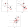 |
Fig. 1. Morphological diagrams for the clusters in our sample with available X-ray Chandra data: (a) c − w, (b) c − P3/P0, and (c) w − P3/P0. Vertical and horizontal dashed lines are adapted from Cassano et al. (2010a): c = 0.2, w = 0.012, and P3/P0 = 1.2 × 10⁻⁷. The red circles represent radio halos, black squares clusters without radio halos, and black triangles clusters with mini halos. The values of the parameters plotted here are listed in Paper I, Table 5. Clusters that are explicitly mentioned in the text are labelled in red. |
Figure 1 shows that only ∼60% of merging clusters host radio halos, confirming previous studies (e.g., Cassano et al. 2013; Bonafede et al. 2017). This suggests that mergers are not the unique players in the formation of radio halos (Brunetti & Jones 2014). One major player is the mass of the clusters that sets the amount of energy released during merger events. To investigate the role of the cluster mass in the radio halo merger connection, we split the clusters into two subsamples according to the median mass value of M500 = 7 × 10¹⁴ M⊙, which guarantees equal statistics in each subsample. We focus on c and w because they are the most robust parameters to define the dynamical state of clusters and they are also determined with much higher accuracy with respect to the power ratios (Paper I and references therein). Figure 2 shows that the fraction of merging clusters without radio halos is ∼20% in high-mass systems, while it is ∼65% in low-mass objects. If we attempt to interpret this evidence in the context of turbulent re-acceleration models, it is the consequence of the fact that massive and merging systems form radio halos emitting up to high frequency, while merging events in low-mass clusters may not induce enough turbulence to accelerate particles up to the energies necessary to emit radiation at GHz frequency (Cassano et al. 2006, 2010a). In this scenario a large fraction of these lower mass merging clusters should host USSRHs (e.g., Brunetti et al. 2008; Cassano et al. 2012).
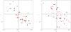 |
Fig. 2. c − w diagram for low-mass (left) and high-mass (right) clusters. Symbols are the same as in Fig. 1. |
Figure 2 also shows that the two clusters with radio halos that appear dynamically relaxed from the morphological parameters (A2142 and A2261) are both in the high-mass bin. This suggests that, in massive clusters, a minor merger may be sufficient to generate radio halos even though the X-ray morphology of the cluster does not look extremely disturbed, whilst low-mass systems need major mergers introducing a larger amount of turbulent energy in the ICM to accelerate electrons and produce radio diffuse emission.
4. Radio power–mass diagram
In this section we investigate the distribution of clusters, with and without radio halos, in the radio power–mass diagram. The values of P1.4 GHz and M500 are listed in Table 1 of Paper I.
All radio halos in the sample, with the exception of three USSRHs, namely A1132 (Wilber et al. 2018), RXCJ1514.9-1523 (Giacintucci et al. 2011), and RXCJ1314.4-2515 (Venturi et al. 2007), have radio powers measured at 1.4 GHz. For these three USSRHs, which have been measured only at low radio frequency, we extrapolated their 1.4 GHz radio powers with the estimated spectral index and we adopted a conservative uncertainty of 30–50%, corresponding to a variation in α of 0.3–0.4.
4.1. Fitting procedure
We followed the fitting procedure outlined in Cassano et al. (2013). Specifically, we fit a power-law relation in the log–log space by adopting the BCES linear regression algorithms (Akritas & Bershady 1996) that take measurement errors in both variables into account. We fitted the observed P1.4 GHz−M500 data points with a power law in the form
 (1)
(1)
where A and B are the intercept and the slope of the correlation, respectively.
Considering Y = log(P1.4 GHz) − 24.5 and X = log(M500) − 14.9, and having a sample of N data points (Xi, Yi) with errors (σXi, σYi), the raw scatter of the correlation can be estimated as
 (2)
(2)
where
 (3)
(3)
Since we are dealing with a limited sample, we obtain a sampled regression line that can deviate from the ‘true’ (unknown) regression line. To evaluate the 95% confidence region of the best-fit relation, that is to say the area that has a 95% probability of containing the true regression line, we calculated the 95% confidence interval of the mean value of Y, ⟨Y⟩. For a given X, this is ⟨Y⟩ ± ΔY, where
![Mathematical equation: $$ \begin{aligned} \Delta Y=\pm 1.96 \sqrt{\left[\sum _{i=0}^N\dfrac{(Y_i-Y_m)^2}{N-2}\right]\left[\dfrac{1}{N}+\dfrac{(X-X_m)^2}{\sum\nolimits_{i=0}^N(X_i-X_m)^2}\right]} .\end{aligned} $$](/articles/aa/full_html/2021/03/aa39208-20/aa39208-20-eq4.gif) (4)
(4)
Here Ym = BXi + A and  for each observed Xi.
4.2. Results of the fitting
Different fitting methods may give different results (e.g., Isobe et al. 1990); therefore, it is important to choose the most suitable regression method depending on the data in hand. Based on previous studies (e.g., Cassano et al. 2013; Martinez Aviles et al. 2016), we expect the correlation between the radio power of radio halos and the mass of clusters to be steep and the radio powers to show a large scatter around the correlation. The large scatter is due to the superposition of clusters with different merging histories, in different phases of the merger events, and with different radio spectra (e.g., Donnert et al. 2013). Thus, it is reasonable to treat the radio power as the dependent variable and use the Y|X fitting method, which minimises the residuals in the Y variable. Another possibility, is to assume that both variables are quasi-independent and treat them symmetrically, using either the bisector method, which represents the bisector between the Y|X and X|Y regression lines, or the orthogonal method, which minimises the orthogonal distances. All these methods are available among the BCES linear regression algorithms (Akritas & Bershady 1996). In the following we report the results obtained with the Y|X and bisector methods.
We show the distribution of radio halos and USSRHs in our sample (which we will refer to as the statistical sample) in the radio power–mass diagram in the left panel of Fig. 3, together with the best-fit line for radio halos only obtained with the BCES Y|X method (see figure caption). In line with previous findings (e.g., Cassano et al. 2013), USSRHs and candidate USSRHs are on or below the correlation. Even considering only radio halos with classical spectra, we note a significant scatter around the correlation. A possible source of the scatter is a different emitting volume of the halos. For example, in Cuciti et al. (2018) we found two small radio halos lying below the correlation. In these cases it is reasonable to expect that they have a synchrotron emissivity similar to that of larger radio halos, but they are less luminous simply because the total luminosity is produced in a smaller volume. To investigate this we measured the radii of the radio halos as  , where Rmin and Rmax are the maximum and minimum radii measured on the 3σ isophote, respectively (Cassano et al. 2007)2. We show the distribution of (RH/R500)3, which is proportional to the volume of radio halos, in the right panel of Fig. 3. The majority of radio halos are distributed around (RH/R500)3 = 0.06 − 0.15.
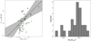 |
Fig. 3. Radio power–mass diagram and volume distribution of the radio halos of the statistical sample. Left: P1.4 GHz − M500 diagram. Black filled circles represent radio halos; green empty circles represent USSRHs and candidate USSRHs. The small radio halos are labelled. The best-fit relation obtained with the BCES Y|X method and excluding USSRHs is shown with its 95% confidence region. The best-fit parameters are B = 3.92 ± 0.79 and A = −0.15 ± 0.10. Right: distribution of the volumes of the radio halos, scaled for R500. The four clusters lying on the left tail, separated from the main distribution, are A3411, Z0634, A2218, and A1689. |
There are four radio halos whose volumes are ∼6−20 times smaller than the average radio halos in our sample. They are in the clusters Z0634, A3411, A1689, and A2218, and they are all underluminous with respect to the correlation (Fig. 3, left). Interestingly, the size of these four small radio halos roughly coincides with the threshold value between radio halos and mini halos (RH ≈ 0.2 × R500) defined by Giacintucci et al. (2017). On the other hand, no halos with volumes larger than 5−6 times that of the average halos are found.
Since the radio luminosity of these four radio halos is generated in a much smaller volume, their radio power cannot be directly compared to the power of giant (RH ∼ Mpc) radio halos3. Also, their radio power cannot be directly compared to the upper limits because upper limits are derived using RH = 500 kpc by choice (corresponding to about RH/R500 ∼ 0.4 for the typical masses and redshift in our sample). If we inject the fake radio halos on smaller scales, the upper limits would be deeper (Brunetti et al. 2007). Therefore, we removed them from the radio luminosity mass diagram and we performed the fit again.
The correlation for the statistical sample without small radio halos is shown in the left panel of Fig. 4, and in the top panel of Table 1 we report the best-fit parameters obtained with the BCES Y|X and bisector methods, together with those from a 5000 bootstrap resampling analysis (see Akritas & Bershady 1996). We also report the raw scatter of the correlation and the Spearman coefficient, rs, which is a measure of the monotonicity of the relationship between two variables 4 (Spearman 1904). We note that the bootstrap confidence intervals are quite large, meaning that the fitting is likely undetermined. This can be a consequence of the cut in mass at M500 ≥ 6 × 10¹⁴ M⊙ of our sample, which implies a small mass range (<0.4 in log space) to estimate the correlation coefficients.
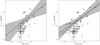 |
Fig. 4. P1.4 GHz − M500 diagram for the clusters of the statistical sample (left) and extended sample (right). Black filled circles are radio halos, arrows are upper limits, and green empty circles are USSRHs or candidate USSRHs. The black line and grey shadowed region show the best-fit relations (using the BCES Y|X method) and the 95% confidence region to radio halos only. For a clear comparison, also shown is the best-fit relation (right panel, dashed line) obtained for the statistical sample (left panel). |
Fitting parameters.
To evaluate the possible effect of this cut on the regression analysis, we performed Monte Carlo simulations (see Appendix A). We randomly distributed a number of clusters with masses in the range M500 = (1−16) × 1014 M⊙ on a known correlation (the true correlation, which we assume to extend as a power law also at low masses) and we applied a fixed scatter in both Y and X to distribute them around the correlation. Then we selected from the distribution only clusters with M500 ≥ 6 × 10¹⁴ M⊙. We repeated these two steps 500 times, and each time we performed the linear regression with the three methods mentioned above, comparing the resulting slopes with the true one. We found that, in the presence of a steep correlation with a fairly large scatter, all the fitting methods tend to give steeper slopes once the cut in the X variable is introduced. In particular, the orthogonal method is the most affected by the presence of the cut, giving the most significant deviations from the true slopes. According to our Monte Carlo simulations we expect the true correlation to be ∼0.2 − 0.3 flatter with respect to what we find in our sample if we focus on the Y|X method, and if we assume the scatter to be predominantly on the Y-axis (see Fig. A.1, bottom left).
We attempted to mitigate the limitation due to the narrow range in mass spanned by the clusters of the statistical sample by considering also an ‘extended’ sample, resulting from the combination with a subsample from Cassano et al. (2013) and Martinez Aviles et al. (2016). In particular, we added only clusters in the same redshift range of our sample (six radio halos). Since one of the goals of this section is to study the distribution of radio halos and upper limits in the radio power–mass diagram (see Sect. 4.4), we also added the upper limits (five) from Cassano et al. (2013) in the same redshift range of our sample. The properties of these additional clusters are listed in Table 2. We note that all six of these radio halos have radio powers measured at 1.4 GHz. This allows us to study the scaling relation with larger statistics and, more importantly, within a wider mass range.
Properties of the added clusters.
The results obtained by applying the fitting procedure to the radio halos of the extended sample are summarised in the bottom panel of Table 1 and are shown in the right panel of Fig. 4. We note that the bootstrap confidence intervals are now more in agreement with the analytic estimates, meaning that the fitting parameters are now better determined.
Although they agree with each other within the 1σ uncertainties, we note that the correlation derived for the extended sample, is slightly flatter (∼0.3) compared to that derived for the statistical sample. This is in line with the outcome of our Monte Carlo simulations, suggesting that possible biases due to the addition of a small subsample of low-mass clusters from the literature (i.e. the radio brightest ones) are likely marginal. We note, however, that only future studies of statistical samples of galaxy clusters covering a wider range of cluster masses, down to a few 1014 M⊙, have the potential to unambiguously determine the slope of the correlation.
Depending on the regression method used, the slope of the correlation ranges from 2.7 to 3.5. This is consistent with the findings of Cassano et al. (2013) and Martinez Aviles et al. (2016). As a further check, we derived the correlation parameters using the Bayesian regression method LInear Regression in Astronomy (LIRA, Sereno 2016). By default, LIRA treats X as the independent variable and Y as the dependent one. We applied LIRA to the extended sample, excluding the small radio halos and USSRH. We obtained a slope B = 2.85 ± 1.3, which is in fact consistent with the BCES Y|X estimation. The larger uncertainty in the slope estimate with LIRA is due to the fact that this method considers a larger number of parameters with respect to BCES (Sereno 2016).
4.3. Scatter of the correlation and clusters’ dynamics
For all fitting methods, the correlation shows a fairly large scatter (Table 1), slightly larger than that found by Cassano et al. (2013). Different mergers may generate different spectra and a wide range of radio emitting volumes (extension of the turbulent regions), as can be seen in the right panel of Fig. 3. The time evolution of radio halos may also contribute to the scatter of the correlation. Simulations show that the synchrotron emission evolves with the cluster dynamics, increasing in the early stages of the merger when turbulence accelerates electrons, and then decreasing along with the dissipation of turbulence at later merger stages (Donnert et al. 2013). In the radio power–mass plane this induces a migration of clusters from the region of the upper limits to the correlation (or above) and then a progressive dimming of the radio power together with a steepening of the spectrum. Yuan et al. (2015) suggested that the scatter of the radio power–X-ray luminosity correlation can be significantly reduced if the dynamical state of clusters is taken into account. Focusing on the statistical sample, without the additional clusters in Table 2, we show in Fig. 5 the distance (on the P1.4 GHz axis) of radio halos from the correlation versus their X-ray morphological disturbance, measured as the distance from the bisector (the one with positive angular coefficient) of the two dashed lines shown in the c − w diagram (Fig. 1, panel a). We found a clear trend between these two quantities, with radio halos scattered up with respect to the correlation being hosted in more dynamically disturbed clusters. We ran a Spearman test (Spearman 1904) and obtained rs = 0.6 and a probability of no correlation of 1.4 × 10⁻³. Figure 5 suggests that the merger activity has a key role in determining the position of radio halos with respect to the correlation, thus inducing at least part of the large scatter that we observe around the correlation. This is in line with previous findings based on simulations (Donnert et al. 2013).
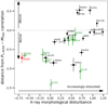 |
Fig. 5. Distance of radio halos from the correlation (BCES Y|X method) vs X-ray morphological disturbance (see Sect. 4.3 for details). Green empty circles represent USSRHs or candidate USSRHs, black squares are clusters with RH/R500 ∼ 0.2, and the red square is A1689, which also has RH/R500 ∼ 0.2 and is undergoing a merger along the line of sight (Andersson & Madejski 2004). |
It is interesting to note that the fraction of USSRHs or candidate USSRHs among the most disturbed clusters in Fig. 5 is ∼20%, whereas it is ∼70% in the less disturbed systems. Although the available statistics on USSRHs is still poor and the information on the spectra is currently not homogeneous, this hint can be interpreted as the consequence of the fact that less energetic mergers induce a low level of turbulence in the ICM, which in turn is not able to accelerate particles up to the energy necessary to emit at ∼GHz frequencies. These less disturbed systems can be either minor mergers or systems in their very late or very early merger state, which are expected to appear more relaxed in the X-rays and to develop steep radio spectra (e.g., Donnert et al. 2013). Interestingly, our results are in line with recent findings suggesting that steep-spectrum halos reside in clusters with high X-ray luminosity relative to that expected from the mass–X-ray luminosity scaling relations, indicating that these systems may be in an earlier state of the merger (Bîrzan et al. 2019). Finally, we also note that small radio halos are predominantly found in less disturbed systems, possibly suggesting that minor mergers dissipate turbulence in smaller volumes.
4.4. Radio bimodality
It is well known that merging clusters with radio halos lie on the radio luminosity–mass (or X-ray luminosity) correlation, while relaxed clusters typically do not host radio halos and their radio power lies well below the correlation (Brunetti et al. 2007, 2009; Cassano et al. 2013). Here we investigate the presence of a bimodal behaviour of clusters with and without radio halos in the radio power–mass diagram focusing on the extended sample without small radio halos (Fig. 4, right). We found that, for clusters with M500 ≳ 5.5 × 10¹⁴ M⊙, almost all the upper limits (∼90%) are below the 95% confidence region of the correlation, confirming previous studies (e.g., Cassano et al. 2013).
To further investigate the radio distribution of clusters with and without radio halos in the P1.4 GHz−M500 diagram, we made use of another method of regression analysis based on the Expectation Maximization (EM) algorithm that is implemented in the ASURV package (Isobe et al. 1986) and that deals with upper limits as ‘censored data’. We applied the EM regression algorithm to the radio halos only and then to the combined radio halos and upper limits. The resulting best fits are shown in Fig. 6 and are summarised in the bottom lines of Table 1. The correlation obtained including upper limits in the fit (dashed line) is much steeper than that derived using only detections. This occurs because the EM algorithm allows for the censored data to assume values smaller than those of the upper limits in an iterative process whose aim is to find a maximum likelihood solution. In addition to the fact that upper limits dominate the cluster statistics at low masses and that most of them are clustered quite below the detections, this leads to a best fit that is significantly different from the best-fit line to radio halos. This suggests the existence of two distinct radio state of galaxy clusters: on-state radio halo clusters that lie on the correlation, and off-state clusters that occupy a different region of the diagram (see also Brown et al. 2011).
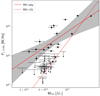 |
Fig. 6. Distribution of radio halos and upper limits in the P1.4 GHz − M500 diagram after removing the five small radio halos. The best-fit relation including only radio halos derived with the EM regression method is shown with its 95% confidence region (red solid line and shadowed region). The dashed line is the EM best-fit relation to radio halos plus upper limits. |
Clusters with upper limits at GMRT frequencies have been extrapolated to 1.4 GHz with α = −1.3. Here we point out that a flatter spectrum (α ∼ −1.1) would make limits only ∼20% shallower with no impact on the conclusions of this section. On the other hand, a steeper spectrum would make limits even deeper, increasing the separation from radio halos.
4.5. Emissivity of radio halos
To study the distribution of the clusters in the radio power mass diagram we removed the smallest radio halos, whose volumes are 6−20 times smaller than the average volume of radio halos in the sample. In general, the different emitting volumes of radio halos may drive a significant fraction of the scatter in the P1.4 GHz−M500 diagram. Therefore, one possibility to remove this effect is to look at the emissivity instead of the radio luminosity. In the following, we focus on the statistical sample without the additional clusters in Table 2.
In Paper I we derived the azimuthally averaged surface brightness radial profile of radio halos and we fitted them with an exponential law to obtain the central surface brightness and the e-folding radius, re. Following Murgia et al. (2009), for these radio halos we calculated the volume averaged emissivity by assuming that their flux density (obtained by integrating the best-fit exponential profile up to 3re) comes from a sphere of radius 3re:
![Mathematical equation: $$ \begin{aligned} J\simeq 7.7\times 10^{-41} (1+z)^{3+\alpha }\ \frac{I_0}{r_e}\,\,\, [\mathrm{erg} \,\mathrm{s} ^{-1}\, \mathrm{cm} ^{-3}\, \mathrm{Hz} ^{-1}] .\end{aligned} $$](/articles/aa/full_html/2021/03/aa39208-20/aa39208-20-eq18.gif) (5)
(5)
In the same way, we calculated the upper limits to the emissivity of clusters without radio halos. In particular, we could use this approach for the upper limits derived in Paper I by injecting an exponential model into the data because we chose re = 500/2.6 = 192 kpc5, and I0 is the one corresponding to the upper limit flux. The values obtained for the emissivity are listed in Table 3 (top panel).
Emissivity of radio halos and upper limits.
We were able to derive the emissivity with this approach only for radio halos with a single peak and a regularly decreasing brightness (about half of the radio halos in our sample). Here we estimate the emissivity for the remaining radio halos, assuming that the measured flux comes from a sphere of radius RH, where RH is derived as in Sect. 4.2. In Fig. 7 we show RH, as derived in Sect. 4.2, as a function of re for the radio halos that have a radial profile available. The value of RH appears to be well correlated with re, in particular, a simple least-squares fit gives log(RH) = 1.12 × log(re)+0.18. We used this relation to infer re for the remaining radio halos, and we estimated I0 by assuming that the measured flux corresponds to the integral of an exponential function up to RH. To estimate the emissivity of the upper limits taken from the literature, we assumed re = 192 kpc to be consistent with the upper limits derived in Paper I. We note that if we used the correlation shown in Fig. 7 to estimate re for the literature upper limits, assuming RH = 500 kpc, we would obtain an offset in the emissivity of less than 10%. We list the values of the emissivity for the remaining radio halos and upper limits in the bottom panel of Table 3.
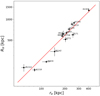 |
Fig. 7. Radio halo radius (RH) measured as in Sect. 4.2 vs e-folding radius (re) of the clusters with available surface brightness radial profile. The best-fit line is shown in red. |
We show the distribution of radio halos and upper limits in the emissivity–mass diagram in Fig. 8. In this plot we do not show the four upper limits at z > 0.31 because, although they are similar to the rest of the upper limits in terms of flux, their luminosity and emissivity is significantly higher (Eq. (5)), meaning that the sensitivity of our current observations does not put stringent upper limits at high redshift. For consistency, we also removed the two halos at z > 0.31 (A1351 and R2003). This is the first time that a systematic study of the emissivities of radio halos is performed in a statistical sample. We found that upper limits have emissivity that is ∼10 times lower than the bulk of radio halos. The apparent bimodality shown in the right panel of Fig. 8 is currently driven by the sensitivity of our observations (which sets the level of our upper limits) and can reflect two possible intrinsic distributions. First, the emissivity of clusters without radio halos is close to the upper limit value, meaning that the distribution is truly bimodal, and that future more sensitive observations should be able to detect these radio halos. Second, the emissivity of clusters without radio halos is for the most part much lower than the upper limits, and in this case the upper limits would represent a tail of the radio halos emissivities extending down to 1–2 orders of magnitude below and the cluster would be lifted up from the tail to the bulk of radio halos as a consequence of merger events. Looking at this second point with deeper observations in the future we will be able to provide valuable information on the evolution of halos and on the level of the hadronic contribution (see Cassano et al. 2012).
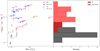 |
Fig. 8. Emissivity vs mass diagram (left) and emissivity distribution (right). The red circles are radio halos with available radial profile, while the blue squares are the remaining radio halos. Upper limits derived in Paper I injecting an exponential model are represented with black arrows, while upper limits from the literature are the grey arrows. |
5. Occurrence of radio halos
To measure the occurrence of radio halos as a function of the cluster mass, we focus on the statistical sample. The great majority of the galaxy clusters with radio upper limits are below the 95% confidence level spanned by the radio power–mass correlation (Fig. 4, right); we classify these clusters as non-radio halos. In five cases (A1914, A115, PSZ1 G205.07-6294, A1763, and A2390), clusters are classified as non-radio halos from the literature using deep radio observations; although no upper limits were derived, we also classified these cases as non-radio halos. However, there are two upper limits consistent with the correlation in our sample, and four clusters for which we were not able to derive upper limits due to problems in the observations. Moreover there are five candidate radio halos in the sample. These 11 clusters have uncertain classification. We consider two cases: a ‘reduced sample’, which does not include the uncertain cases at all, and the total sample, where we assume that candidate radio halos actually host radio halos and clusters without good upper limits do not host radio halos. We point out that a random assignment of radio halos among the 11 uncertain clusters would lead to almost to the same measured fractions of halos.
Following the procedure adopted in Cuciti et al. (2015), we split the sample into two mass bins and measured the fraction of clusters with radio halos, fRH, in the low-mass bin (LM, M < Mlim) and in the high-mass bin (HM, M > Mlim). In particular, we used Mlim = 8 × 10¹⁴ M⊙ for consistency with our previous study. With this partition we have the following:
-
60 clusters in the LM bin, of which 9 host radio halos, 5 host USSRHs or candidate USSRHs, 3 host radio halos with RH/R500 ∼ 0.2, and 11 with uncertain classification (5 candidate radio halos and 6 clusters without solid upper limit);
-
15 clusters in the HM bin, of which 5 host radio halos, 5 host USSRHs or candidate USSRHs, 1 hosts a radio halo with RH/R500 ∼ 0.2.
In total, there are four small radio halos in the statistical sample; one of the small halos shown in Fig. 3 belongs to the extended sample. In order to take into account the uncertainty on the derived fractions of radio halos associated with the statistical error on the masses, we used a Monte Carlo approach. Specifically, we randomly extracted the mass of each cluster from a Gaussian distribution having median value μ = M500 and standard deviation σ = σM500, where M500 and σM500 are the values of the mass and associated error as reported in the Planck catalogue6. Then we split the clusters into the two bins with Mlim = 8 × 10¹⁴ M⊙ and calculated the fractions of radio halos. We repeated this procedure 1000 times and we assumed that the fraction of radio halos in each bin is the mean of the resulting distribution and the error is the standard deviation. With this approach we obtained that the fraction of clusters with radio halos in the LM bin is fRH = 37 ± 2% in the total sample and fRH = 35 ± 2% in the reduced sample, while in the HM bin fRH = 67 ± 6% both in the total and reduced samples. We thus confirmed the existence of a drop in fRH at low-mass systems with a complete mass-selected sample of galaxy clusters (≳80% mass completeness).
5.1. Comparison with theoretical expectations
We used the model developed by Cassano & Brunetti (2005) and Cassano et al. (2006) to derive the formation probability of radio halos as a function of the mass of the host cluster in the redshift range of our sample (z = 0.08−0.33). These models take into account the formation history of galaxy clusters using merger trees and calculate the generation of turbulence, the particle acceleration, and the synchrotron spectrum during the clusters’ lifetime. These models currently offer the unique possibility to calculate the expected occurrence of radio halos to be compared with observations. The basic idea of these models is that the synchrotron spectra of radio halos are characterised by a steepening frequency, νs, which is the result of the competition between turbulent acceleration and radiative (synchrotron and inverse-Compton) losses. In general, νs≳ GHz is expected in the most massive clusters undergoing major mergers, while less energetic merger events that involve clusters with smaller masses are expected to form radio halos with lower values of νs. These radio halos should show extremely steep spectra (α < −1.5, with S(ν) ∝ να) when observed at approximately gigahertz frequencies, and they are expected to constitute the class of USSRHs. The possibility to detect a radio halo is thus related to the observing frequency, νobs; in particular, the spectral steepening challenges the detection of radio halos with νs < νobs.
We calculated the theoretical formation probability of radio halos with νs > 600 MHz and νs > 140 MHz as a function of the cluster mass in the redshift range z = 0.08 − 0.33 (Fig. 9). The uncertainties in the model (red and blue shadowed regions) are calculated with Monte Carlo extractions from the large number of theoretical merger trees and take into account the statistical error introduced by the limited size of our observed sample. The value of νs > 600 MHz can be considered as a reference frequency for both VLA 1.4 GHz and GMRT 610 MHz observations, that constitute the great majority of the available radio observations for the clusters in our sample.
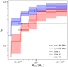 |
Fig. 9. Expected fraction of clusters with radio halos with steepening frequency νs > 600 MHz and νs > 140 MHz in the redshift range 0.08 < z < 0.33 (red and blue lines, respectively). Shadowed regions represent the uncertainty on the model predictions taking into account the statistical error associated with the limited size of the observed sample. Calculations have been performed for the following choice of model parameters: b = 1.5, ⟨B⟩ = 1.9 μG (where B = ⟨B⟩×(M/⟨M⟩)b), and the fraction of energy channelled into particle acceleration ηt = 0.2 (see Cassano et al. 2012, and references therein). The observed fraction of clusters with radio halos in the two mass bins is overlaid (black lines) and refers to the three cases in Table 4 for the total sample. The dots represent the average mass of the clusters in the bins. |
In order to properly compare these expectations with our observations, we need to take two main points into account. First, some of the USSRHs and candidate USSRHs observed in our sample may have νs < 600 MHz; in this case, they should be counted as radio halos only in the comparison with model expectations with νs > 140 MHz. Second, a limitation of these models is that the size of the emitting volume is fixed at RH = 500 kpc7. However, the volume of the small radio halos in our sample is 6−20 times smaller than the volume assumed in the models, implying that the occurrence of radio halos in these situations is biased low in models because the turbulence generated in a smaller volume is artificially spread in a Mpc3 causing a decline in particle acceleration efficiency and νs. Therefore, in the comparison between models and observations, one option is to consider small radio halos as non-radio halos or, in alternative, as USSRHs.
For these reasons we consider three possibilities for the comparison with calculations that assume a value of the minimum steepening frequency νs: (i) small radio halos and USSRHs are non-radio halo clusters (i.e. their steepening frequency is assumed to be lower than the minimum steepening frequency in the considered models); (ii) small radio halos are non-radio halo clusters, whereas USSRH are; (iii) both small radio halos and USSRHs are considered radio halo clusters. To simplify the comparison, here we consider candidate USSRHs as USSRHs, although future observations might not confirm their steep spectra. In Table 4 we report the observed fractions of radio halos in these three cases both for the reduced sample and the total sample. These fractions are derived with the Monte Carlo approach described in Sect. 5. We show the comparison between the predicted and observed fraction of radio halos as a function of mass in Fig. 9. The difference between the total and the reduced samples in terms of fRH is marginal (Table 4), thus for clarity in Fig. 9 we report only the total sample.
Observed fraction of radio halos.
In spite of the basic assumption adopted in the model, there is a remarkable agreement between the observed fraction of clusters with radio halos in the two mass bins and the model expectation with νs > 600 MHz. In particular, case (i) can be considered the lower limit inferred from observations in the comparison with this particular model, essentially because a fraction of the USSRHs and candidate USSRHs in our sample might have νs > 600 MHz. Conversely, case ii) can be considered the upper limit in this comparison. On the other hand, when attempting a comparison with models with νs > 140 MHz (blue line), cases (ii) and (iii) provide the most relevant observational constraints. However, these constraints are driven by observations at higher frequencies (600–1400 MHz, Paper I) and may have lost a significant number of USSRHs in our sample. As a consequence, the discrepancy between the model predictions for νs > 140 MHz and the observed fraction of radio halos in the LM bin implies that a number of radio halos in low-mass clusters should be discovered with future low-frequency observations.
These models are anchored to the observed mass distribution function of clusters (Press & Schechter 1974) and to the rate of mergers that is predicted by the standard ΛCDM model; consequently, since the occurrence of radio halos decreases at low mass, the number of merging clusters without radio halos (when observed at frequencies >600 MHz) should increase. In agreement with that, in Sect. 3 we find that the fraction of merging clusters without radio halos is much higher in low-mass clusters (∼65%) than in high-mass clusters (∼20%). At the same time, this model predicts that a fraction of these mergers will generate radio halos emitting at lower frequencies (e.g., Cassano et al. 2006, 2010b, 2012, see also Fig. 9). Consequently, we expect that a large fraction of the merging systems in our sample that do not show radio halos in the GMRT and JVLA images will be USSRHs that can be detected by low-frequency observations. In this respect, with the LOw-Frequency Array (LOFAR, van Haarlem et al. 2013) we will perform the statistical analysis of radio halos at low frequencies and the comparison with the results presented in this paper will give unprecedented insight into the formation and evolution of radio emission in clusters.
6. Summary and conclusions
We presented the first statistical analysis of radio halos in a mass-selected sample of 75 galaxy clusters. Clusters were selected from the Planck SZ catalogue (Planck Collaboration XXIX 2014) with mass M500 ≥ 6 × 10¹⁴ M⊙ and redshift z = 0.08 − 0.33. The radio and X-ray data analysis of these clusters are described in Paper I. In the following we summarise the main steps and results of the statistical analysis performed in this paper.
We combined the radio information on the clusters in our sample with the dynamical information coming from the X-ray data analysis (see Paper I) in the morphological diagrams (Fig. 1). We find that more than the 90% of radio halos are in merging galaxy clusters, whereas less than 10% are in non-merging systems. As expected, not all the merging clusters host a radio halo. Interestingly, the fraction of merging clusters without radio halos is ∼65% in low-mass clusters, whereas it is ∼20% in high-mass ones (Fig. 2). This is in line with turbulent re-acceleration models predicting that merging events in low-mass systems may not induce enough turbulence to accelerate particles emitting at ∼GHz frequencies.
We confirmed the presence of a correlation between the radio power of radio halos and the mass of the host clusters (Fig. 4). However, we showed that the narrow range of masses of our sample is a significant limitation if our aim is to constrain the slope of the correlation (Appendix A). Therefore, we considered an extended sample, made by the combination of our statistical sample with a subsample of clusters from Cassano et al. (2013) and Martinez Aviles et al. (2016). Depending on the fitting method, the slope of the correlation ranges between 2.7 to 3.5. This result is consistent with previous findings (Cassano et al. 2013; Martinez Aviles et al. 2016).
We investigated the possible connection between the scatter of the correlation and the different dynamical state of clusters. We found a clear trend between the distance from the P1.4 GHz − M500 correlation and the dynamical disturbance of clusters (Fig. 5). This indicates that the large scatter around the correlation is at least partly due to the complex mix of merging histories in the diagram. Interestingly, the great majority of radio halos in less disturbed systems are USSRHs (Fig. 5), suggesting that less energetic merger events may not be sufficient to produce radio halos emitting at ∼ GHz frequencies. Additionally, some of these clusters may be in a late stage of merger where the X-ray morphology appears relaxed and the radio halo spectrum has steepened.
Although the scatter of the correlation is relatively large and the bimodality is less evident, limits still occupy a different region of the P1.4 GHz − M500 diagram, being below the 95% confidence region of the correlation (Figs. 4 and 6).
For the first time, we studied the emissivity of radio halos in a mass-selected sample of clusters. In the emissivity the scattering induced in the radio luminosities by the different emitting volume is reduced. We find a clear separation between radio halos and upper limits with limits lying more than five times below the bulk on radio halos in the emissivity-mass diagram.
Following Cuciti et al. (2015), we measured the occurrence of radio halos in two mass bins: M < 8 × 10¹⁴ M⊙ and M ≥ 8 × 10¹⁴ M⊙. We found that the fraction of clusters with radio halos is ∼70% in high-mass clusters and ∼35% in low-mass clusters, thus confirming the presence of a drop in the fraction of radio halos in low-mass systems.
We used the model developed by Cassano & Brunetti (2005) to compare the observed and predicted fraction of radio halos as a function of mass (Fig. 9). Although these models have some limitations that require a careful comparison, we showed that there is good agreement between the theoretical expectations and our observations. The combination of the decline of occurrence and increase of the fraction of merging clusters without radio halos in lower mass clusters suggests that a population of USSRH should be discovered among those systems with low-frequency observations.
M500 is the mass enclosed in a sphere with radius R500, defined as the radius within which the mean mass over-density of the cluster is 500 times the cosmic critical density at the cluster redshift.
For elongated radio halos (Rmax ≫ Rmin) we multiplied RH by a factor  to take the ellipticity of radio halos into account.
An additional possibility is that these radio halos appear small because our observations did not recover their entire extension. However, this would also imply that a large fraction of their flux is lost by our observations and that their luminosities are biased low compared to those of the other halos in our sample.
rs = −1 implies a perfect monotonically decreasing relation, rs = +1 implies a perfect monotonically increasing relation, and rs = 0 implies no correlation.
The value 2.6 was derived in Bonafede et al. (2017) to convert RH into re.
Since the errors on the masses are not symmetric, here we assume σM500 to be equal to the largest error.
RH = 500 kpc corresponds to RH/R500 ∼ 0.4 for the typical masses of our cluster sample, which is consistent with the average and/or typical sizes of radio halos in our sample (Fig. 3, right).
Acknowledgments
The authors thank the anonymous referee for the useful comments which improved the presentation of the paper. V. C. acknowledges support from the Alexander von Humboldt Foundation. R. J. vW. acknowledges support from the VIDI research programme with project number 639.042.729, which is financed by the Netherlands Organisation for Scientific Research (NWO). R. K. acknowledges the support of the Department of Atomic Energy, Government of India, under project no. 12-R&D-TFR-5.02-0700. Basic research in radio astronomy at the Naval Research Laboratory is supported by 6.1 Base funding. S. E. acknowledges financial contribution from the contracts ASI-INAF Athena 2019-27-HH.0, “Attività di Studio per la comunità scientifica di Astrofisica delle Alte Energie e Fisica Astroparticellare” (Accordo Attuativo ASI-INAF n. 2017-14-H.0), INAF mainstream project 1.05.01.86.10, and from the European Union’s Horizon 2020 Programme under the AHEAD2020 project (grant agreement n. 871158). G. W. P. acknowledges the support of the French space agency, CNES. The National Radio Astronomy Observatory is a facility of the National Science Foundation operated under cooperative agreement by Associated Universities, Inc. We thank the staff of the GMRT that made these observations possible. GMRT is run by the National Centre for Radio Astrophysics of the Tata Institute of Fundamental Research. The scientific results reported in this article are based in part on data obtained from the Chandra Data Archive. This research has made use of the NASA/IPAC Extragalactic Database (NED) which is operated by the Jet Propulsion Laboratory, California Institute of Technology, under contract with the National Aeronautics and Space Administration.
References
- Akritas, M. G., & Bershady, M. A. 1996, ApJ, 470, 706 [Google Scholar]
- Andersson, K. E., & Madejski, G. M. 2004, ApJ, 607, 190 [Google Scholar]
- Andrade-Santos, F., Jones, C., Forman, W. R., et al. 2017, ApJ, 843, 76 [NASA ADS] [CrossRef] [Google Scholar]
- Basu, K. 2012, MNRAS, 421, L112 [Google Scholar]
- Bîrzan, L., Rafferty, D. A., Cassano, R., et al. 2019, MNRAS, 487, 4775 [NASA ADS] [CrossRef] [Google Scholar]
- Bonafede, A., Intema, H., Brüggen, M., et al. 2015, MNRAS, 454, 3391 [Google Scholar]
- Bonafede, A., Cassano, R., Brüggen, M., et al. 2017, MNRAS, 470, 3465 [Google Scholar]
- Brown, S., Emerick, A., Rudnick, L., & Brunetti, G. 2011, ApJ, 740, L28 [Google Scholar]
- Brunetti, G., & Jones, T. W. 2014, Int. J. Mod. Phys. D, 23, 1430007 [Google Scholar]
- Brunetti, G., Venturi, T., Dallacasa, D., et al. 2007, ApJ, 670, L5 [Google Scholar]
- Brunetti, G., Giacintucci, S., Cassano, R., et al. 2008, Nature, 455, 944 [NASA ADS] [CrossRef] [Google Scholar]
- Brunetti, G., Cassano, R., Dolag, K., & Setti, G. 2009, A&A, 507, 661 [NASA ADS] [CrossRef] [EDP Sciences] [Google Scholar]
- Buote, D. A. 2001, ApJ, 553, L15 [NASA ADS] [CrossRef] [Google Scholar]
- Cassano, R., & Brunetti, G. 2005, MNRAS, 357, 1313 [NASA ADS] [CrossRef] [Google Scholar]
- Cassano, R., Brunetti, G., & Setti, G. 2006, MNRAS, 369, 1577 [Google Scholar]
- Cassano, R., Brunetti, G., Setti, G., Govoni, F., & Dolag, K. 2007, MNRAS, 378, 1565 [Google Scholar]
- Cassano, R., Brunetti, G., Röttgering, H. J. A., & Brüggen, M. 2010a, A&A, 509, A68 [NASA ADS] [CrossRef] [EDP Sciences] [Google Scholar]
- Cassano, R., Ettori, S., Giacintucci, S., et al. 2010b, ApJ, 721, L82 [Google Scholar]
- Cassano, R., Brunetti, G., Norris, R. P., et al. 2012, A&A, 548, A100 [NASA ADS] [CrossRef] [EDP Sciences] [Google Scholar]
- Cassano, R., Ettori, S., Brunetti, G., et al. 2013, ApJ, 777, 141 [NASA ADS] [CrossRef] [Google Scholar]
- Cuciti, V., Cassano, R., Brunetti, G., et al. 2015, A&A, 580, A97 [NASA ADS] [CrossRef] [EDP Sciences] [Google Scholar]
- Cuciti, V., Brunetti, G., van Weeren, R., et al. 2018, A&A, 609, A61 [NASA ADS] [CrossRef] [EDP Sciences] [Google Scholar]
- Donnert, J., Dolag, K., Brunetti, G., & Cassano, R. 2013, MNRAS, 429, 3564 [NASA ADS] [CrossRef] [Google Scholar]
- Giacintucci, S., Dallacasa, D., Venturi, T., et al. 2011, A&A, 534, A57 [NASA ADS] [CrossRef] [EDP Sciences] [Google Scholar]
- Giacintucci, S., Markevitch, M., Cassano, R., et al. 2017, ApJ, 841, 71 [Google Scholar]
- Giovannini, G., Tordi, M., & Feretti, L. 1999, New A, 4, 141 [Google Scholar]
- Govoni, F., Markevitch, M., Vikhlinin, A., et al. 2004, ApJ, 605, 695 [Google Scholar]
- Isobe, T., Feigelson, E. D., & Nelson, P. I. 1986, ApJ, 306, 490 [Google Scholar]
- Isobe, T., Feigelson, E. D., Akritas, M. G., & Babu, G. J. 1990, ApJ, 364, 104 [Google Scholar]
- Kale, R., Venturi, T., Giacintucci, S., et al. 2013, A&A, 557, A99 [NASA ADS] [CrossRef] [EDP Sciences] [Google Scholar]
- Kale, R., Venturi, T., Giacintucci, S., et al. 2015, A&A, 579, A92 [NASA ADS] [CrossRef] [EDP Sciences] [Google Scholar]
- Kempner, J. C., & Sarazin, C. L. 2001, ApJ, 548, 639 [Google Scholar]
- Liang, H., Hunstead, R. W., Birkinshaw, M., & Andreani, P. 2000, ApJ, 544, 686 [Google Scholar]
- Lovisari, L., Forman, W. R., Jones, C., et al. 2017, ApJ, 846, 51 [NASA ADS] [CrossRef] [Google Scholar]
- Markevitch, M., & Vikhlinin, A. 2001, ApJ, 563, 95 [Google Scholar]
- Markevitch, M., Ponman, T. J., Nulsen, P. E. J., et al. 2000, ApJ, 541, 542 [Google Scholar]
- Martinez Aviles, G., Ferrari, C., Johnston-Hollitt, M., et al. 2016, A&A, 595, A116 [NASA ADS] [CrossRef] [EDP Sciences] [Google Scholar]
- Murgia, M., Govoni, F., Markevitch, M., et al. 2009, A&A, 499, 679 [NASA ADS] [CrossRef] [EDP Sciences] [Google Scholar]
- Nagai, D. 2006, ApJ, 650, 538 [Google Scholar]
- Owers, M. S., Nulsen, P. E. J., & Couch, W. J. 2011, ApJ, 741, 122 [Google Scholar]
- Planck Collaboration XXIX. 2014, A&A, 571, A29 [NASA ADS] [CrossRef] [EDP Sciences] [Google Scholar]
- Press, W. H., & Schechter, P. 1974, ApJ, 187, 425 [NASA ADS] [CrossRef] [Google Scholar]
- Rossetti, M., Eckert, D., De Grandi, S., et al. 2013, A&A, 556, A44 [NASA ADS] [CrossRef] [EDP Sciences] [Google Scholar]
- Rossetti, M., Gastaldello, F., Eckert, D., et al. 2017, MNRAS, 468, 1917 [NASA ADS] [CrossRef] [Google Scholar]
- Santos, J. S., Rosati, P., Tozzi, P., et al. 2008, A&A, 483, 35 [NASA ADS] [CrossRef] [EDP Sciences] [Google Scholar]
- Sereno, M. 2016, MNRAS, 455, 2149 [Google Scholar]
- Sommer, M. W., & Basu, K. 2014, MNRAS, 437, 2163 [Google Scholar]
- Spearman, C. 1904, The. Am. J. Psychol., 15, 72 [Google Scholar]
- van Haarlem, M. P., Wise, M. W., Gunst, A. W., et al. 2013, A&A, 556, A2 [NASA ADS] [CrossRef] [EDP Sciences] [Google Scholar]
- van Weeren, R. J., de Gasperin, F., Akamatsu, H., et al. 2019, Space Sci. Rev., 215, 16 [NASA ADS] [CrossRef] [Google Scholar]
- Venturi, T., Giacintucci, S., Brunetti, G., et al. 2007, A&A, 463, 937 [NASA ADS] [CrossRef] [EDP Sciences] [Google Scholar]
- Venturi, T., Giacintucci, S., Dallacasa, D., et al. 2008, A&A, 484, 327 [NASA ADS] [CrossRef] [EDP Sciences] [Google Scholar]
- Venturi, T., Rossetti, M., Brunetti, G., et al. 2017, A&A, 603, A125 [NASA ADS] [CrossRef] [EDP Sciences] [Google Scholar]
- Wilber, A., Brüggen, M., Bonafede, A., et al. 2018, MNRAS, 473, 3536 [NASA ADS] [CrossRef] [Google Scholar]
- Yuan, Z. S., Han, J. L., & Wen, Z. L. 2015, ApJ, 813, 77 [Google Scholar]
Appendix A: Test BCES
The sample of galaxy clusters analysed in this paper is selected from the Planck SZ catalogue imposing a cut in mass at M500 ≥ 6 × 10¹⁴ M⊙. As a consequence, our sample contains clusters within a relatively narrow range of masses (6 ≤ M500 < 16 × 1014 M⊙, with only one cluster with M500 > 11 × 1014 M⊙). In order to test whether and how such a cut influences the correlation parameters derived with the BCES methods, we performed Monte Carlo simulations. We randomly distributed 60, 100, or 1000 points in the X − Y diagram on a correlation in the form Y = slope × X. We used five values for the slope: 3.5, 4, 4.5, 5, 5.5. We worked in log space and we chose values for the X variable similar to those that we are dealing with in our cluster sample, but in a wider range (X is in the range 14 − 15.2, with X = log(M500)). Here the assumption is that the scaling remains a power law also extending to lower masses. We associated a random error with these points, both in X and Y, in line with the errors that we have in our mass and radio power measurements. Then we distributed the points around the correlation following two approaches:
-
(a)
We assumed that the scatter in X is only statistical scatter, while the scatter in Y is both statistical and intrinsic;
-
(b)
We assumed that the raw scatter (statistic and intrinsic) is orthogonal with respect to the correlation line.
In both cases the value of the scatter that we introduced was chosen to be similar to the value observed in our sample. We repeated the random distribution 500 times for each value of the slope, and each time we performed the BCES analysis described in Sect. 4.1. We found that all the BCES methods are able to recover the true slope of the correlation with <10% discrepancies (the discrepancy decreases as the number of points increases).
As a second test, after applying the scattering, we selected only points with X ≥ 14.77, corresponding to the cut in mass of our sample. An example of the distribution of points in the X − Y diagram after the cut in the X variable is shown in Fig. A.1, top left. In this case the true slope of the correlation is 4.5 and the scatter follows approach a). The initial distribution is made of 60 clusters, which allows us to obtain a similar number of points to our sample once the cut is applied. The top right panel of Fig. A.1 shows the distribution of the slopes given by the three different fitting methods for the 500 Monte Carlo trials. In Fig. A.1, bottom left, we show the difference between the recovered and the true slope as a function of the true slope. We repeated this test using an orthogonal scatter (approach b). Results are shown in Fig. A.1, bottom right panel. Our analysis suggests that a cut in the X variable influences the results of the fitting using the BCES algorithms. In particular, regardless of how the points are scattered around the correlation, the orthogonal method always gives steeper slopes with the largest uncertainties. Which fitting method performs better depends on how the scatter is implemented. Since it is not trivial to know the best way to describe the scatter around the correlation, in this paper we report the values obtained with the Y|X and the bisector methods. In addition, we point out that the bisector method allows us to better compare our results with previous works (e.g., Cassano et al. 2013).
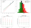 |
Fig. A.1. Top panel: left: one example of the 500 Monte Carlo runs with true correlation slope 4.5 and X cut at 14.77 (corresponding to a mass cut of 6 × 10¹⁴). Right: distribution of the recovered slopes with the bisector (black), orthogonal (red), and Y|X (green) methods. The vertical lines represent the mean value of the recovered slopes and the dashed line is the true slope. These mean values of the slopes are used to draw the correlation lines in left panel. Bottom panels: difference between recovered and true slope as a function of the true slope for the three fitting methods. The dots represent the mean values of the distributions, while the error bars are as large as the standard deviation of the distribution of the recovered slopes. The horizontal grey line represents the case where the recovered slope matches the true slope. In the left panel we used the Y scatter, in the right panel the orthogonal scatter. |
All Tables
All Figures
|
Fig. 1. Morphological diagrams for the clusters in our sample with available X-ray Chandra data: (a) c − w, (b) c − P3/P0, and (c) w − P3/P0. Vertical and horizontal dashed lines are adapted from Cassano et al. (2010a): c = 0.2, w = 0.012, and P3/P0 = 1.2 × 10⁻⁷. The red circles represent radio halos, black squares clusters without radio halos, and black triangles clusters with mini halos. The values of the parameters plotted here are listed in Paper I, Table 5. Clusters that are explicitly mentioned in the text are labelled in red. |
| In the text | |
|
Fig. 2. c − w diagram for low-mass (left) and high-mass (right) clusters. Symbols are the same as in Fig. 1. |
| In the text | |
|
Fig. 3. Radio power–mass diagram and volume distribution of the radio halos of the statistical sample. Left: P1.4 GHz − M500 diagram. Black filled circles represent radio halos; green empty circles represent USSRHs and candidate USSRHs. The small radio halos are labelled. The best-fit relation obtained with the BCES Y|X method and excluding USSRHs is shown with its 95% confidence region. The best-fit parameters are B = 3.92 ± 0.79 and A = −0.15 ± 0.10. Right: distribution of the volumes of the radio halos, scaled for R500. The four clusters lying on the left tail, separated from the main distribution, are A3411, Z0634, A2218, and A1689. |
| In the text | |
|
Fig. 4. P1.4 GHz − M500 diagram for the clusters of the statistical sample (left) and extended sample (right). Black filled circles are radio halos, arrows are upper limits, and green empty circles are USSRHs or candidate USSRHs. The black line and grey shadowed region show the best-fit relations (using the BCES Y|X method) and the 95% confidence region to radio halos only. For a clear comparison, also shown is the best-fit relation (right panel, dashed line) obtained for the statistical sample (left panel). |
| In the text | |
|
Fig. 5. Distance of radio halos from the correlation (BCES Y|X method) vs X-ray morphological disturbance (see Sect. 4.3 for details). Green empty circles represent USSRHs or candidate USSRHs, black squares are clusters with RH/R500 ∼ 0.2, and the red square is A1689, which also has RH/R500 ∼ 0.2 and is undergoing a merger along the line of sight (Andersson & Madejski 2004). |
| In the text | |
|
Fig. 6. Distribution of radio halos and upper limits in the P1.4 GHz − M500 diagram after removing the five small radio halos. The best-fit relation including only radio halos derived with the EM regression method is shown with its 95% confidence region (red solid line and shadowed region). The dashed line is the EM best-fit relation to radio halos plus upper limits. |
| In the text | |
|
Fig. 7. Radio halo radius (RH) measured as in Sect. 4.2 vs e-folding radius (re) of the clusters with available surface brightness radial profile. The best-fit line is shown in red. |
| In the text | |
|
Fig. 8. Emissivity vs mass diagram (left) and emissivity distribution (right). The red circles are radio halos with available radial profile, while the blue squares are the remaining radio halos. Upper limits derived in Paper I injecting an exponential model are represented with black arrows, while upper limits from the literature are the grey arrows. |
| In the text | |
|
Fig. 9. Expected fraction of clusters with radio halos with steepening frequency νs > 600 MHz and νs > 140 MHz in the redshift range 0.08 < z < 0.33 (red and blue lines, respectively). Shadowed regions represent the uncertainty on the model predictions taking into account the statistical error associated with the limited size of the observed sample. Calculations have been performed for the following choice of model parameters: b = 1.5, ⟨B⟩ = 1.9 μG (where B = ⟨B⟩×(M/⟨M⟩)b), and the fraction of energy channelled into particle acceleration ηt = 0.2 (see Cassano et al. 2012, and references therein). The observed fraction of clusters with radio halos in the two mass bins is overlaid (black lines) and refers to the three cases in Table 4 for the total sample. The dots represent the average mass of the clusters in the bins. |
| In the text | |
|
Fig. A.1. Top panel: left: one example of the 500 Monte Carlo runs with true correlation slope 4.5 and X cut at 14.77 (corresponding to a mass cut of 6 × 10¹⁴). Right: distribution of the recovered slopes with the bisector (black), orthogonal (red), and Y|X (green) methods. The vertical lines represent the mean value of the recovered slopes and the dashed line is the true slope. These mean values of the slopes are used to draw the correlation lines in left panel. Bottom panels: difference between recovered and true slope as a function of the true slope for the three fitting methods. The dots represent the mean values of the distributions, while the error bars are as large as the standard deviation of the distribution of the recovered slopes. The horizontal grey line represents the case where the recovered slope matches the true slope. In the left panel we used the Y scatter, in the right panel the orthogonal scatter. |
| In the text | |
Current usage metrics show cumulative count of Article Views (full-text article views including HTML views, PDF and ePub downloads, according to the available data) and Abstracts Views on Vision4Press platform.
Data correspond to usage on the plateform after 2015. The current usage metrics is available 48-96 hours after online publication and is updated daily on week days.
Initial download of the metrics may take a while.