| Issue |
A&A
Volume 647, March 2021
|
|
|---|---|---|
| Article Number | A115 | |
| Number of page(s) | 10 | |
| Section | Extragalactic astronomy | |
| DOI | https://doi.org/10.1051/0004-6361/202038971 | |
| Published online | 18 March 2021 | |
Measuring accretion disk sizes of lensed quasars with microlensing time delay in multi-band light curves
Institute of Physics, Laboratory of Astrophysique, École Polytechnique Fédérale de Lausanne (EPFL), Observatoire de Sauverny, 1290 Versoix, Switzerland
e-mail: This email address is being protected from spambots. You need JavaScript enabled to view it.
Received:
19
July
2020
Accepted:
20
October
2020
Abstract
Time-delay cosmography in strongly lensed quasars offers an independent way of measuring the Hubble constant, H0. However, it has been proposed that the combination of microlensing and source-size effects, also known as microlensing time delay, can potentially increase the uncertainty in time-delay measurements as well as lead to a biased time delay. In this work, we first investigate how microlensing time delay changes with assumptions on the initial mass function (IMF) and find that the more massive microlenses produce the sharper distributions of microlensing time delays. We also find that the IMF has a modest effect on the magnification probability distributions. Second, we present a new method to measure the color-dependent source size in lensed quasars using the microlensing time delays inferred from multi-band light curves. In practice, the relevant observable is the differential microlensing time delays between different bands. We show from a simulation using the facility as Vera C. Rubin Observatory that if this differential time delay between bands can be measured with a precision of 0.1 days in any given lensed image, the disk size can be recovered to within a factor of 2. If four lensed images are used, our method is able to achieve an unbiased source measurement within an error on the order of 20%, which is comparable with other techniques.
Key words: gravitational lensing: strong / gravitational lensing: micro / quasars: general
© ESO 2021
1. Introduction
A strong gravitational lens effect occurs when light emitted from a background source is deflected due to the gravitational potential of a foreground object, resulting in multiple lensed images of the source. In particular, strongly lensed quasars provide us with a powerful tool to study galaxy evolution and to infer cosmological parameters. The careful use of the positions and magnification ratios of the lensed images allow one to quantify the level of substructures in the lensing galaxy, which are directly related to how galaxies form and evolve and to the nature of the dark matter they contain (e.g., Harvey et al. 2020; Suyu et al. 2012; Dalal & Kochanek 2002). As quasars are variable sources, the time delays between the lensed images allow us to determine the time-delay distance in each system, which is inversely proportional to the Hubble constant H0 (e.g., Refsdal 1964; Suyu et al. 2010). Over the years, time-delay cosmography with lensed quasars has achieved high precision on H0 measurements, as carried out by the H0LiCOW1 Collaboration (H0 Lenses in COSMOGRAIL2’s Wellspring; Suyu et al. 2017; Wong et al. 2020). Future progress will be reported in the new series of TDCOSMO3 papers (Time-delay COSMOgraphy; Millon et al. 2020a).
One of the key ingredients for time-delay cosmography is to measure precise and accurate time delays. These are regularly obtained by the COSMOGRAIL and TDCOSMO Collaborations from optical light curves for a rapidly increasing number of lensed quasars (e.g., Millon et al. 2020b,c; Bonvin et al. 2018, 2019a). On the other hand, Tie & Kochanek (2018, hereafter TK18) propose a possible source of bias in time-delay measurements, called microlensing time delay, which also affects lensed supernovae (Bonvin et al. 2019b). This extra positive or negative delay may emerge when microlensing caustics unequally magnify different parts of the quasar accretion disk (or supernova shell). To estimate microlensing time delay in a lensed quasar, we require high precision of lens modeling and the structure of an accretion disk.
The traditional techniques to study the inner components of quasars are microlensing and reverberation mapping. Both approaches are used to infer the structure of the quasar accretion disk, which is vital to understanding the growth and evolution of super massive black holes (SMBHs). In the first case, measuring the microlensing amplitude variability using light curves or single epoch spectra has served this purpose for decades (e.g., Schechter & Wambsganss 2002; Kochanek 2004; Morgan et al. 2010, 2018; Dai et al. 2010; Cornachione et al. 2020; Rojas et al. 2014, 2020). In the second case, reverberation mapping commonly monitors non-lensed quasars in multiple filters (e.g., Fausnaugh et al. 2016; Jiang et al. 2017; Mudd et al. 2018; Yu et al. 2020). Under the condition that the disk size is larger at a longer wavelength, the time delays between the light curves in different bands provide a measurement for the size (τ ∝ R ∝ λ4/3): the larger the disk, the longer the delay. Similarly, we can apply the same methodology as in reverberation mapping to “lensed quasars”, if light curves of the lensed images are available in several filters. Such data should be available in the near future from the Vera C. Rubin Observatory (hereafter Rubin; Ivezić et al. 2019).
In this work, we investigate microlensing time delay and propose a new method to measure the disk size in lensed quasars using multi-filter light curves. This is complementary to the traditional microlensing work that only considers the amplitude of the microlensing and not the delay and distortion that it introduces in the light curves. We use RX J1131−1231 (hereafter J1131) as an example, as it has displays that are prominent microlensing events. The redshifts of the lens and source are zL = 0.295 and zS = 0.658, respectively (Sluse et al. 2003). Based on the Hβ line width which was measured by Sluse et al. (2003), Dai et al. (2010) estimated the black hole mass to be Mbh = (1.3 ± 0.3) × 108 M⊙. Table 1 lists the lensing parameters used to generate magnification maps, corresponding to a macro lens model with a stellar mass fraction of f⋆ = 0.2 relative to a pure de Vaucouleurs model (Dai et al. 2010; Tie & Kochanek 2018).
Microlensing model parameters of J1131: κ, γ, κ⋆/κ, and μth at each lensed image position from TK18.
The paper is organized as follows. The microlensing time delay with various initial mass functions is described in Sect. 2. Section 3 presents our method for estimating the source size using microlensing time delay and our conclusions are described in Sect. 4.
2. Microlensing time delay in IMFs
Reliable time-delay measurements between the strongly lensed images are key to obtaining a precise H0 measurement. However, in the presence of microlensing, a lensed image is affected by an excess of time delay, either positive or negative, which is due to the microlens magnification pattern. This additional delay is not necessarily cancelled out when measuring cosmological time delays in several lensed quasars as a result of the different excesses at multiple images. TK18 proposed a microlensing time delay (MLTD) for the first time and computed the microlensing time delays statistically for the following two lensed quasars: J1131 and HE 0435−1223. The mean bias of the distribution of microlensing delays is on the order of a day; furthermore, for peculiar geometrical configurations, this bias can reach several days. Other lensed quasars display a nearly negligible microlensing time delay (Bonvin et al. 2018; Birrer et al. 2019; Chen et al. 2019; Shajib et al. 2020). A method has been presented in Chen et al. (2018) to account for the effect of the microlensing time delay in cosmological inference with strongly lensed quasars.
Estimating MLTD requires a microlensing magnification map and a model for the source accretion disk that is affected by microlensing. In this work, we follow the recipe provided by TK18 but we further investigate the impact of the adopted initial mass function (IMF) on magnification maps and MLTD. In this section, we describe how we generate magnification maps in Sect. 2.1, and recap the basics of MLTD in Sect. 2.2. We present the MLTD distributions with various IMFs in Sect. 2.3.
2.1. Magnification maps
We generated the magnification maps using GPU-D (Vernardos & Fluke 2014), which includes a graphics processing unit (GPU) implementation of the inverse ray–shooting technique (Kayser et al. 1986). The default setup of the IMF is uniform with 1.0 M⊙. In this work, we expand the range of mean microlens masses ⟨M⋆⟩ from 0.1 M⊙ to 3.0 M⊙. Except for the uniform mass distribution, we adopt a Salpeter mass function with ⟨M⋆⟩ = 0.3 M⊙ and the ratio between upper and lower bounds of the mass interval, r = Mupper/Mlower = 100, which is favored by galaxy-scale lenses (e.g., Kochanek 2004; Oguri et al. 2014). The Chabrier mass function with ⟨M⋆⟩ = 0.3 M⊙ is also taken into account in this work (Chabrier 2003).
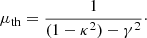
The microlensing parameters are taken from TK18, listed in Table 1, that is to say the surface mass density for the macro model, κ (lensing convergence), the shear of the macro model, γ, the fraction of the mass under the form of stars, κ⋆/κ, and the macro-magnification at the position of the quasar images, thus
 (1)
(1)
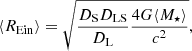
All magnification maps are 20⟨REin⟩ on a side with 8192 pixels, which are sizable in this work, where
 (2)
(2)
which depends on the angular diameter distances from the observer to the lens DL, from the observer to the source DS, and from the lens to the source DLS. For J1131,  .
.
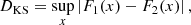
As an example, in Fig. 1, we show the magnification maps for image A with the uniform, Salpeter, and Chabrier IMFs. For r = 1, this is equivalent to a delta function, corresponding to the uniform mass function. The magnification probability distributions are shown in the top panels of Fig. 2. In order to measure the similarities between different distributions, we adopt the Kolmogorov–Smirnov statistic for each pair of cumulative distribution functions F1(x) and F2(x), expressed as
 (3)
(3)
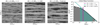 |
Fig. 1. Examples of magnification maps for image A of RX J1131−1231 in the three left panels, with the corresponding IMFs in the right panel. All maps are 20⟨REin⟩ on a side, corresponding to 81922 pixels. The r factor corresponds to the ratio between the upper and lower bound of the mass interval, so that r = 1 indicates single-mass IMFs. The magnification probability distributions are shown in Fig. 2. |
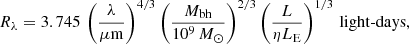
where supx is the supremum of the set of distances. We note that DKS converges at 0 when two distributions are the same. The results are shown in the bottom panels of Fig. 2. Given a sample size of 100, the condition at the confidence level of 95% to reject that two distributions are the same is DKS ≳ 0.2. Since the size of the magnification map is scaled by the mean stellar mass, once the shape of the IMF is fixed, an alternation of ⟨M⋆⟩ does not vary the map. For the Salpeter and Chabrier mass functions, we note that the distributions are slightly deviated due to some larger caustics. Although the details of the microlensing pattern do change, we find that the magnification probability distributions are insensitive to the choice of the IMFs, but they are not independent of them. This result is in line with previous work (e.g., Wambsganss 1992; Lewis & Irwin 1995; Wyithe & Turner 2001; Schechter et al. 2004; Vernardos & Fluke 2013; Mediavilla et al. 2015; Jiménez-Vicente & Mediavilla 2019).
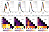 |
Fig. 2. Top: magnification probability distribution of each lensed image, i.e. the histogram of the pixels in the maps (see Fig. 1). Bottom: Kolmogorov–Smirnov statistic of each distribution pair (see Eq. (3)). In each case, the corresponding μ is indicated in the middle. The Salpeter and Chabrier mass functions have slightly deviated distributions. Small DKS shows that the probability distributions are insensitive to the chosen mean stellar mass or IMF, but they are not independent of them. |
2.2. Microlensing time delay
We now recall the basics of MLTD and describe the model used to generate simulations. For the lensed source, we consider a nonrelativistic thin-disk model, emitting black-body radiation (Shakura & Sunyaev 1973), where the central source is assumed to be a “lamp post” located closely above the black hole (Cackett et al. 2007; Krolik et al. 1991; Wanders et al. 1997; Collier et al. 1998; Starkey et al. 2016). The temperature profile on a disk follows a simple form of T(R) ∝ R−3/4. Although some observations support the shallower profile, such as a slim disk (Abramowicz et al. 1988; Cornachione & Morgan 2020), a simple model should be allowed since MLTD is subtle and created by the variable flux (Tie & Kochanek 2018). Under the thin-disk assumption, the disk radius where the disk temperature matches the photon wavelength (kT = hc/λ) can be expressed as
 (4)
(4)
where L/LE is the luminosity in units of the Eddington luminosity, LE, and η is the accretion efficiency (e.g., Morgan et al. 2010). In ignoring the inner edge of the “face-on” disk in the simple lamp post model, the average MLTD can be derived using Eq. (10) of Tie & Kochanek (2018) or Eq. (6) of Chan et al. (2020), which are reproduced here for convenience:
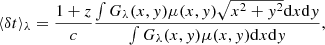 (5)
(5)
where μ(x, y) is the magnification map projected on the source plane with the coordinates x, y, and Gλ(ξ) is the first derivative of the luminosity profile of the disk which can be expressed as
![Mathematical equation: $$ \begin{aligned} G_{\lambda }(\xi )=\frac{\xi \exp (\xi )}{\left[\exp (\xi )-1\right]^2}, \end{aligned} $$](/articles/aa/full_html/2021/03/aa38971-20/aa38971-20-eq7.gif) (6)
(6)
where  (see Tie & Kochanek 2018; Chan et al. 2020, for a detailed explanation of the coordinate system). For a given geometrical configuration and accretion disk model, we can thus compute the mean excess of microlensing time delay ⟨δt⟩λ for a given source position and magnification pattern. In the absence of microlensing, all the lensed images share the same amount of lag ⟨δt⟩λ, geo = 5.04(1 + zS)Rλ/c, which is called “geometric delay” or “lamp-post delay”. In Fig. 3, we show how ⟨δt⟩λ changes when the microlensing effect is added. In each panel we highlight the effective radius 5.04(1 + zS)Rλ = c ⋅ ⟨δt⟩λ, geo = 2.315 light-day. The overall results are summarized in the lower right panel of the figure, which clearly shows how microlensing distorts the probability distribution of time delays.
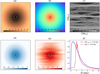 |
Fig. 3. Illustration of the distortion of the probability distribution of time delays with and without the microlensing effect. Panel a: geometrical time lag of the disk, which is simply |
The mean delay ⟨δt⟩λ changes by varying the magnification pattern. In Fig. 4, we present ⟨δt⟩λ as a function of disk size Rλ, when a source is placed in ten random positions on a magnification map, corresponding to ten sub-magnification patterns with a size of 5⟨REin⟩, labeled from Sim0 to Sim9. The purely geometrical delay ⟨δt⟩λ, geo is found, that is to say the delay in the absence of microlensing. In the figure, we again consider Rλ = 0.277 light-day as fiducial value. As in Fig. 4, the effective radius 5.04(1 + zS)Rλ = 2.315 light-day is also shown. When the inner circle is magnified, ⟨δt⟩λ is shorter, as shown in Sim1 and Sim6. On the contrary, when the inner circle is demagnified, ⟨δt⟩λ is longer, as shown in Sim2 and Sim3.
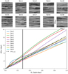 |
Fig. 4. Top: examples of magnification patterns spanning each 5⟨REin⟩, assuming the IMF ⟨M⋆⟩ = 0.3 M⊙ and r = 100. Bottom: source size Rλ and mean delay ⟨δt⟩λ for each realization of the magnification pattern. The dotted line in black corresponds to the relation without microlensing, i.e. the geometric delay. The white circles in the top panels represent the effective radius 5.04(1 + zS)Rλ = 2.315 light-day, and the vertical black line in the bottom panel indicates Rλ = 0.277 light-day (see text). |
2.3. The effect of IMF on microlensing time delay distribution
It is not possible to know the exact microlens pattern and we need to proceed in a statistical way. For a given geometrical configuration of the accretion disk model, we can then compute the mean excess of microlensing time delay ⟨δt⟩λ at any given source position, as described in Sect. 2.2. By varying the magnification pattern, we can draw the probability distribution of microlensing time delay ⟨δt⟩λ for each lensed image. Practically, we can convolve a magnification map and disk light distribution using Eq. (5), and we then obtain the mean delay ⟨δt⟩λ map, given a source at each pixel of the magnification map. Although the magnification probability distribution is insensitive to IMFs, as described in Sect. 2.1, it is natural to ask whether the IMFs have an impact on the ⟨δt⟩λ distribution. In the following section, as a reference, we choose the filter that is currently being used for cosmological time delay by the TDCOSMO Collaboration (e.g., Millon et al. 2020a), that is the Rc filter. For J1131, this corresponds to the observed wavelength λobs = (1 + zS) × λ = 6517.25 Å. Given an Eddington ratio of L/LE = 0.1 and a radiative efficiency of η = 0.1, we obtain the disk size Rλ = 0.277 light-day.
In Fig. 5, we present the microlensing time delay distributions of ⟨δt⟩λ − ⟨δt⟩λ, geo for different IMFs in the top panels. This quantity is the excess of the microlensing time delay with respect to the purely geometric time delay, since there is an absence of ⟨δt⟩λ, geo when measuring cosmological time delay. For smaller mean stellar masses, we notice that the distribution becomes wider and has a slightly larger mean. Since microlensing time delay is estimated by the convolution of the magnification map and disk light profile, the ⟨δt⟩λ maps are similar to but smoother than the magnification map (see Figs. 2−5 in Tie & Kochanek 2018). In other words, smaller caustics located across the disk lead to a higher probability at producing small delays and thus the probability distribution becomes wider. Furthermore, since we can scale the size unit to  , a smaller mean mass correlates with a larger source size, which not only results in the width but also in the offset of the MLTD distribution. In this work, we extend ⟨M⋆⟩ ranging by a factor of 30, corresponding to Rλ ranging by a factor of 5.5. This offset can be evident at small mean masses or larger source sizes, which agrees with the result in TK18. Same as in Fig. 2, the Kolmogorov–Smirnov statistics are shown in the bottom panel. We note that DKS values of MLTD are generally larger than those of μ. This shows that the MLTD distributions are more sensitive to the mean stellar masses, resulting from the equivalent changes in source size and, in particular, for the sharper distributions, which occur when ⟨M⋆⟩ = 3.0 M⊙ and also in image D. However, a sharper distribution also indicates that the MLTD has less of an impact on the cosmological time delays.
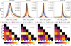 |
Fig. 5. Top: probability distribution of microlensing time delay of each lensed image. Bottom: Kolmogorov–Smirnov statistic of each distribution pair (see Eq. (3)). In each case the corresponding mean time delay is indicated in the middle. |
3. Disk measurement via microlensing time delay
The reverberation mapping of continuum light curves is of much importance when measuring the physical size of quasar accretion disks (Mudd et al. 2018; Yu et al. 2020). Measuring the relative lags between the multi-band light curves allowed us to derive the color-dependent disk size, given a combination of an accretion disk model in the context of the lamp-post model for the intrinsic variations of the quasar. In principle, this method can be applied to lensed quasars, and especially the quadruply-imaged ones that display four realizations of microlensing maps. However, the light curves of the lensed images are distorted by the microlensing with respect to each other, hence affecting the distributions for ⟨δt⟩λ and Rλ, as shown in Fig. 4.
In this section, we propose a new method for estimating the disk size using microlensing time delay given multi-band light curves. We see this method both as a way to study quasar physics at very small scales (light days) and as a way to mitigate the impact of microlensing time delay when measuring H0. We illustrate our method in Fig. 6 and give the technical details in Sect. 3.1 along with our main findings in Sect. 3.2.
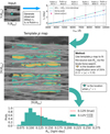 |
Fig. 6. Flow chart of our procedure to simulate multi-band microlensing curves and how to analyze them. The top row shows how we simulated our “observed data” given a fiducial source, the magnification pattern, and microlensing magnification, μ = −4.28. The negative magnification indicates that the image is at the saddle point. The “template magnification map” used to analyze the data is shown in the middle panel (see text), where preselected locations used in fitting the source size are shown in yellow. These correspond to areas where the microlensing magnification matches the fiducial one with ≤25% error. In the end, we only kept the regions where fitting the source size gives χ2 < 1. These are shown in green and were used to produce the distribution of measured source size Rλ0 in the bottom row. For reference purposes, we provide the true (fiducial) size as a red vertical line. |
3.1. Simulation and method
We provide a flowchart of our method in Fig. 6. The flowchart can be split into three parts. We first started to simulate “observed delays”, which is illustrated in the top row of the figure and is explained below. We then analyzed the simulated data by creating microlensing maps and by selecting possible locations where the microlensing time delays match the observed ones. This corresponds to the middle panel of the figure. Finally, we processed the outputs of this selection and display them in the bottom row of the figure. Each of these steps are detailed below.
We first simulated the data set by taking Rubin’s filters, consisting in light curves in six bands, that is u, g, r, i, z, and y. The observed wavelengths for each filter are indicated in the top-right subplot of Fig. 6 for the specific case of image A in J1131, which we consider to be a textbook case in this work. To do this, we put a disk on a given magnification pattern with a size of 5⟨REin⟩, as shown in the top-left subplot, and we generated the mean delay, ⟨δt⟩λ, in six Rubin-like bands. In this work, we disregard the peculiar velocity of the system, assuming static magnification patterns, which is achievable when delays can be measured within a short period (Millon et al. 2020b). The (simulated) observed delay measurements were calculated by τλ = ⟨δt⟩λ − ⟨δt⟩λ0, relative to a reference band (λ0), and they can be seen in the top-right subplot. These are our simulated data and we choose the bluest possible band as a reference, as this is where the accretion disk is the smallest. The relation of the resulting delays as a function of wavelength, both with and without a microlensing effect, are shown. In this specific simulation, the delays become longer in the presence of microlensing because there is more microcaustic falling in the outer parts of disk than in the inner parts, but of course the opposite case is possible, depending on where the microcaustics fall within the accretion disk. In practice, measuring such short delays is not trivial given the small source size, even for non-lensed quasars. Most traditional curve shifting techniques may underestimate the source size by up to ∼30%, even in the absence of microlensing (Chan et al. 2020). This is because they often only consider a shift between the unmagnified light curves in each band and not the actual distortion caused by the convolution of the lamp-post disk profile by the light profile of the accretion disk. In the following, we assume that the delays are measured without bias and we then illustrate how to use them to infer the accretion disk size.
Second, in the same spirit as reverberation mapping, we use a series of (correctly measured) multi-filter light curves for a given lensed image, and we perform a least-square fit following:
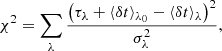 (7)
(7)
where σλ is the room mean square (rms) precision of the measurement, which we assume to be 0.1 days here. Unlike traditional reverberation mapping methods, there is no analytical relation between the delays at different wavelengths, since the relation ⟨δt⟩λ ∝ λ4/3 breaks down due to microlensing (see Sect. 2.2 and Fig. 4). However, as shown in Fig. 4, we can predict relations between ⟨δt⟩λ and Rλ ∝ λ4/3 for a given disk model and magnification pattern. To do so, we generated a large magnification map as a template, as shown in the middle row of Fig. 6. We note that the input magnification pattern used to produce the simulated data was not taken from this template magnification map. We then placed an accretion disk on this template magnification map and we sought after possible locations where the magnification may allow for one to match the observed delays τλ. In practice, we first produced a series of relations between Rλ and ⟨δt⟩λ at all positions in the template map by convolving with the corresponding accretion disk model of size Rλ. We then compared with the observed delays τλ with this series of predicted relations between Rλ and ⟨δt⟩λ, using Eq. (7). Each fit provides us with the best-fit of ⟨δt⟩λ0 at the specific location, and hence we can infer the corresponding Rλ0. This “brute-force” search is time consuming, since it is necessary to scan over all positions on the template magnification map. Of course, the use of GPUs may speed this process up, but another way to work around this is to reduce the number of fitting processes by preselecting the possible positions on the template map that reproduce the microlensing magnification. In the case of image A of J1131, this is μ = −4.28, which also corresponds to the center of the input magnification pattern in the top-left subplot of Fig. 6.
In practice, this magnification is measurable on real data either using long light curves (Millon et al. 2020c) or flux anomalies (e.g., More et al. 2017). Here, we conservatively take the microlensing magnification with typical error bars of 25%. This allowed us to reduce the number of locations on the map to ≲10% of what it would take without preselection, although relaxing this criterion is insensitive to the posterior size distribution. These plausible solutions are shown in the figure; they are the only places where we needed to perform the least-square fitting.
The last step is to collect those positions with small χ2 given a threshold (χ2 < 1 in this work), shown in the template magnification map. In the bottom subplot, we draw the probability distribution of the source size estimation and highlight the mean and 1σ error bars for the 50th, 16th, and 84th percentiles of the distribution, respectively. The distribution shows that we are able to recover the source size within the 1σ error.
3.2. Result
With our analysis chain in hand, we assigned the disk source at ten random positions of a magnification map to generate the observed delays (top panels in Fig. 4) and see whether we can recover the source size regardless of the magnification pattern. We note that the input magnification patterns are produced using stellar masses with a mean mass of ⟨M⋆⟩ = 0.3 and assuming r = 100 for the IMF. We tested three source sizes by varying the quasar luminosity over a broad range, that is L/LE = 1.0, 0.1, and 0.01, corresponding to Rλ0 = 0.277, 0.129, and 0.060 light-day, respectively, according to Eq. (4). We then prepared a template magnification map in order to perform brute-force fitting. Hereafter, we adopt three different IMFs which are common and accepted in microlensing works. The first two share the same mean stellar mass of ⟨M⋆⟩ = 0.3, but they use r = 100 and r = 1. The last one has ⟨M⋆⟩ = 1.0 and r = 1. Each magnification template map has 20⟨REin⟩ on a side. Although, here, we only present the result with one realization of the template for each IMF; the test for more realizations is described in Appendix A.
The distribution of size measurements for each simulation is presented in Fig. 7. Each data point and error bar correspond the 50th, 16th, and 84th percentiles of the probability distribution, as shown in the bottom panel of Fig. 6. We then compared the measurements with the true value and therefore show the ratio between the measurement and true value Rmeas/Rtrue. It is immediately striking that the measurement is insensitive to the choice of the IMFs in the template microlensing map. This is particularly important since so far determining the IMF of the lensing galaxy toward the line of sight to a lensed quasar image has not been possible. Still, we were able to recover the disk size within a factor of 2, regardless of the input size.
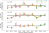 |
Fig. 7. Ratio between source size measurement and true size for ten simulations of microcaustic networks with lensing properties corresponding to quasar image A of J1131. Using L/LE = 1.0, 0.1, and 0.01 for three assumed luminosities, the source size corresponds to Rλ0 = 0.277, 0.129, and 0.060 light-day, respectively (see Eq. (2)). The unbiased measurements are labeled as black lines for reference purposes. Each time, three typical IMFs are implemented and labeled in the top right corner. The results are clearly insensitive to the choice of the lens galaxy IMF. |
A nice advantage of a lensed quasar over a non-lensed one where reverberation mapping is usually performed is that we have two or even four sets of multi-band light curves for each object. In the ideal case of fours images, this allows us to measure the source size four times simultaneously, as we illustrate in Fig. 8. Here we only employ the template magnification maps with ⟨M⋆⟩ = 0.3 and r = 100, since Fig. 7 shows that the measurement is insensitive to the IMFs. After marginalizing over all fours measurements, as shown in gray, we were able to recover the source within the error ∼20%. When a source is smaller, the error is also slightly smaller, since the microlensing time delay is closer in amplitude to the geometric delay. The uncertainty of measurement of image A is larger than other lensed images as a result of the stronger microlensing effect. Of course, it is also possible to apply this method to doubly lensed quasars. Although this gives only access to two sets of multi-band light curves, microlensing is less effective in the brighter image of doubles in general.
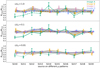 |
Fig. 8. Same as Fig. 7, but now using the four images of J1131, which are labeled in the top right corner. The template magnification maps were adopted using the IMF of ⟨M⋆⟩ = 0.3, r = 100 and the marginalized result using four images is shown in the gray. |
For clarity, the entire above study was carried out for a face-on accretion disk. Other disk configurations with inclinations and position angles can also be considered and are explored in Appendix A. In this work, we choose the exceptional condition (rms 0.1 days) to demonstrate this method, and achieve the comparable source-size measurement with that from other techniques. We note that high accuracy and the precision of delay is likely to be necessary for this method, since the microlensing time delays between filters are very short in general. The requirement of the delay measurement is beyond the scope of this work.
4. Conclusion and discussion
TK18 first introduced the notion of microlensing time delay, and they argue that time delay measurements in lensed quasars can be biased due to different parts of the accretion disk being microlensed in different ways. Since the effect depends on the source size and since the source size is a chromatic quantity, we propose measuring multi-band time delays in lensed quasars and using them to measure the size the accretion disk under the assumption of the lamp-post model and given a model for the accretion disk light profile.
We investigate the microlensing time delay using different IMFs, using the well-studied lensed quasar J1131 as an example, and we show that the magnification probability distribution is insensitive to the IMF in the lensing galaxy. The probability distribution of the microlensing time delay is wider when decreasing the mean stellar mass of the microlenses. This trend follows accordingly as increasing the source size, as the microlensing analysis can be scaled by the mean mass of microlenses. Still, for typical mean stellar masses ⟨M⋆⟩ between 0.3 and 1.0 M⊙, the distributions for microlensing time delays are nearly indistinguishable. This makes it possible to measure disk sizes even under the assumption of a poorly known IMF or mean stellar masses, which is contrary to traditional microlensing methods, where the source size is very degenerate with the properties assumed for the microlenses.
We propose a new method to measure the disk size of quasars, based on the continuum reverberation mapping method but applied to strongly lensed quasars, assuming the static magnification pattern. To illustrate the method, we assume Rubin-like light curves providing time delays in six filters with each an rms precision of 0.1 days and no bias. Assuming that such data can actually be gathered in practice, we find the following.
-
Using the brute-force search on a template magnification map, we are able to recover the disk size within a factor of 2, with the multi-filter light curves of only one lensed image.
-
This method is insensitive to the IMFs.
-
After marginalizing all measurements of multiple lensed images, we can achieve an unbiased measurement within an error of ∼20%.
The present work sets the basis for a new way of using microlensing time delay in multi-band light curves for astrophysical purposes. Here, we focus on how to measure the size of quasar accretion disks, but our future work will also consider the joint measurements of the cosmological time delay and microlensing time delay, allowing us both to mitigate the impact of microlensing time delay on H0 measurements and to use it to measure quasar accretion disks at the same time. This is particularly relevant in the era of large time-domain and multi-band surveys such as the Rubin Observatory Legacy Survey of Space and Time (LSST).
Acknowledgments
We thank P. Schechter for the useful discussion and the referee for the comments. This work is supported by the Swiss National Science Foundation (SNSF) and by the European Research Council (ERC) under the European Union’s Horizon 2020 research and innovation program (COSMICLENS: grant agreement No 787886).
References
- Abramowicz, M. A., Czerny, B., Lasota, J. P., & Szuszkiewicz, E. 1988, ApJ, 332, 646 [Google Scholar]
- Birrer, S., Treu, T., Rusu, C. E., et al. 2019, MNRAS, 484, 4726 [NASA ADS] [CrossRef] [Google Scholar]
- Bonvin, V., Chan, J. H. H., Millon, M., et al. 2018, A&A, 616, A183 [NASA ADS] [CrossRef] [EDP Sciences] [Google Scholar]
- Bonvin, V., Millon, M., Chan, J. H. H., et al. 2019a, A&A, 629, A97 [NASA ADS] [CrossRef] [EDP Sciences] [Google Scholar]
- Bonvin, V., Tihhonova, O., Millon, M., et al. 2019b, A&A, 621, A55 [NASA ADS] [CrossRef] [EDP Sciences] [Google Scholar]
- Cackett, E. M., Horne, K., & Winkler, H. 2007, MNRAS, 380, 669 [NASA ADS] [CrossRef] [Google Scholar]
- Chabrier, G. 2003, PASP, 115, 763 [Google Scholar]
- Chan, J. H. H., Millon, M., Bonvin, V., & Courbin, F. 2020, A&A, 636, A52 [EDP Sciences] [Google Scholar]
- Chen, G. C. F., Chan, J. H. H., Bonvin, V., et al. 2018, MNRAS, 481, 1115 [NASA ADS] [CrossRef] [Google Scholar]
- Chen, G. C. F., Fassnacht, C. D., Suyu, S. H., et al. 2019, MNRAS, 490, 1743 [Google Scholar]
- Collier, S. J., Horne, K., Kaspi, S., et al. 1998, ApJ, 500, 162 [NASA ADS] [CrossRef] [Google Scholar]
- Cornachione, M. A., & Morgan, C. W. 2020, ApJ, 895, 93 [Google Scholar]
- Cornachione, M. A., Morgan, C. W., Millon, M., et al. 2020, ApJ, 895, 125 [Google Scholar]
- Dai, X., Kochanek, C. S., Chartas, G., et al. 2010, ApJ, 709, 278 [NASA ADS] [CrossRef] [Google Scholar]
- Dalal, N., & Kochanek, C. S. 2002, ApJ, 572, 25 [NASA ADS] [CrossRef] [Google Scholar]
- Fausnaugh, M. M., Denney, K. D., Barth, A. J., et al. 2016, ApJ, 821, 56 [NASA ADS] [CrossRef] [Google Scholar]
- Harvey, D., Valkenburg, W., Tamone, A., et al. 2020, MNRAS, 491, 4247 [Google Scholar]
- Ivezić, Ž., Kahn, S. M., Tyson, J. A., et al. 2019, ApJ, 873, 111 [NASA ADS] [CrossRef] [Google Scholar]
- Jiang, Y.-F., Green, P. J., Greene, J. E., et al. 2017, ApJ, 836, 186 [NASA ADS] [CrossRef] [Google Scholar]
- Jiménez-Vicente, J., & Mediavilla, E. 2019, ApJ, 885, 75 [Google Scholar]
- Kayser, R., Refsdal, S., & Stabell, R. 1986, A&A, 166, 36 [NASA ADS] [Google Scholar]
- Kochanek, C. S. 2004, ApJ, 605, 58 [Google Scholar]
- Krolik, J. H., Horne, K., Kallman, T. R., et al. 1991, ApJ, 371, 541 [NASA ADS] [CrossRef] [Google Scholar]
- Lewis, G. F., & Irwin, M. J. 1995, MNRAS, 276, 103 [NASA ADS] [Google Scholar]
- Mediavilla, E., Jimenez-Vicente, J., Muñoz, J. A., Mediavilla, T., & Ariza, O. 2015, ApJ, 798, 138 [NASA ADS] [CrossRef] [Google Scholar]
- Millon, M., Galan, A., Courbin, F., et al. 2020a, A&A, 639, A101 [CrossRef] [EDP Sciences] [Google Scholar]
- Millon, M., Courbin, F., Bonvin, V., et al. 2020b, A&A, 642, A193 [CrossRef] [EDP Sciences] [Google Scholar]
- Millon, M., Courbin, F., Bonvin, V., et al. 2020c, A&A, 640, A105 [CrossRef] [EDP Sciences] [Google Scholar]
- More, A., Suyu, S. H., Oguri, M., More, S., & Lee, C.-H. 2017, ApJ, 835, L25 [NASA ADS] [CrossRef] [Google Scholar]
- Morgan, C. W., Kochanek, C. S., Morgan, N. D., & Falco, E. E. 2010, ApJ, 712, 1129 [NASA ADS] [CrossRef] [Google Scholar]
- Morgan, C. W., Hyer, G. E., Bonvin, V., et al. 2018, ApJ, 869, 106 [Google Scholar]
- Mudd, D., Martini, P., Zu, Y., et al. 2018, ApJ, 862, 123 [NASA ADS] [CrossRef] [Google Scholar]
- Oguri, M., Rusu, C. E., & Falco, E. E. 2014, MNRAS, 439, 2494 [NASA ADS] [CrossRef] [Google Scholar]
- Refsdal, S. 1964, MNRAS, 128, 307 [NASA ADS] [CrossRef] [Google Scholar]
- Rojas, K., Motta, V., Mediavilla, E., et al. 2014, ApJ, 797, 61 [NASA ADS] [CrossRef] [Google Scholar]
- Rojas, K., Motta, V., Mediavilla, E., et al. 2020, ApJ, 890, 3 [Google Scholar]
- Schechter, P. L., & Wambsganss, J. 2002, ApJ, 580, 685 [NASA ADS] [CrossRef] [Google Scholar]
- Schechter, P. L., Wambsganss, J., & Lewis, G. F. 2004, ApJ, 613, 77 [NASA ADS] [CrossRef] [Google Scholar]
- Shajib, A. J., Birrer, S., Treu, T., et al. 2020, MNRAS, 494, 6072 [Google Scholar]
- Shakura, N. I., & Sunyaev, R. A. 1973, A&A, 24, 337 [NASA ADS] [Google Scholar]
- Sluse, D., Surdej, J., Claeskens, J. F., et al. 2003, A&A, 406, L43 [NASA ADS] [CrossRef] [EDP Sciences] [Google Scholar]
- Starkey, D. A., Horne, K., & Villforth, C. 2016, MNRAS, 456, 1960 [NASA ADS] [CrossRef] [Google Scholar]
- Suyu, S. H., Marshall, P. J., Auger, M. W., et al. 2010, ApJ, 711, 201 [NASA ADS] [CrossRef] [Google Scholar]
- Suyu, S. H., Hensel, S. W., McKean, J. P., et al. 2012, ApJ, 750, 10 [NASA ADS] [CrossRef] [Google Scholar]
- Suyu, S. H., Bonvin, V., Courbin, F., et al. 2017, MNRAS, 468, 2590 [Google Scholar]
- Tie, S. S., & Kochanek, C. S. 2018, MNRAS, 473, 80 [NASA ADS] [CrossRef] [Google Scholar]
- Vernardos, G., & Fluke, C. J. 2013, MNRAS, 434, 832 [NASA ADS] [CrossRef] [Google Scholar]
- Vernardos, G., & Fluke, C. J. 2014, Astron. Comput., 6, 1 [Google Scholar]
- Wambsganss, J. 1992, ApJ, 386, 19 [NASA ADS] [CrossRef] [Google Scholar]
- Wanders, I., Peterson, B. M., Alloin, D., et al. 1997, ApJS, 113, 69 [NASA ADS] [CrossRef] [Google Scholar]
- Wong, K. C., Suyu, S. H., Chen, G. C. F., et al. 2020, MNRAS, 498, 1420 [Google Scholar]
- Wyithe, J. S. B., & Turner, E. L. 2001, MNRAS, 320, 21 [NASA ADS] [CrossRef] [Google Scholar]
- Yu, Z., Martini, P., Davis, T. M., et al. 2020, ApJS, 246, 16 [NASA ADS] [CrossRef] [Google Scholar]
Appendix A: Additional tests
In this section, we present the test on the different realizations of the template magnification map and the test on the tilted disk. From each simulation, we measured the source size with five different realizations of template magnification maps with 20⟨REin⟩ on a side, as labeled with different colors. Each map was generated using the IMF of ⟨M⋆⟩ = 0.3 and r = 100. Figure A.1, which is similar to Fig. 7, shows that size measurements from different realizations agree well. This test also demonstrates that the size of the template maps is large enough for this method.
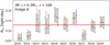 |
Fig. A.1. Source measurement of Image A using different template magnification maps. The source was placed on ten magnification patterns labeled from Sim0 to Sim9. For each simulation, we employed five realizations of templates to measure the source size, as labeled with different colors. The true value is labeled with the red line. |
In this work, we mainly present our result with face-on disks. We further explore the tilted disks with inclination (i) and position angle (PA). The inclination angle is defined as the tilted degree along the line of sight, with i = 0° corresponding to the disk lying in the plane of the sky. The position angle determines an angle between the long axis of the tilted disk and the caustic structures of the magnification maps. Although the observed delays are simulated using a tilted disk, we still employed our method with face-on disk (i = 0° and PA = 0°) to measure the source size. The result is shown in Fig. A.2.
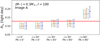 |
Fig. A.2. Source measurement of Image A with different inclinations (i) and position angles (PA) of disk configuration. For each simulation, we employed five realizations of the template magnification map to measure the source size. The true value is labeled with the red line. |
A larger inclination angle or position angle give us slightly larger measurements, resulting from the alignment between the disk and caustics. This result agrees with TK18, finding that the microlensing time delay has a minor dependence on the inclination of the disk and its orientation relative to the caustic networks. Therefore, the assumption of the face-on disk is sufficient to recover the input disk size.
All Tables
Microlensing model parameters of J1131: κ, γ, κ⋆/κ, and μth at each lensed image position from TK18.
All Figures
|
Fig. 1. Examples of magnification maps for image A of RX J1131−1231 in the three left panels, with the corresponding IMFs in the right panel. All maps are 20⟨REin⟩ on a side, corresponding to 81922 pixels. The r factor corresponds to the ratio between the upper and lower bound of the mass interval, so that r = 1 indicates single-mass IMFs. The magnification probability distributions are shown in Fig. 2. |
| In the text | |
|
Fig. 2. Top: magnification probability distribution of each lensed image, i.e. the histogram of the pixels in the maps (see Fig. 1). Bottom: Kolmogorov–Smirnov statistic of each distribution pair (see Eq. (3)). In each case, the corresponding μ is indicated in the middle. The Salpeter and Chabrier mass functions have slightly deviated distributions. Small DKS shows that the probability distributions are insensitive to the chosen mean stellar mass or IMF, but they are not independent of them. |
| In the text | |
|
Fig. 3. Illustration of the distortion of the probability distribution of time delays with and without the microlensing effect. Panel a: geometrical time lag of the disk, which is simply |
| In the text | |
|
Fig. 4. Top: examples of magnification patterns spanning each 5⟨REin⟩, assuming the IMF ⟨M⋆⟩ = 0.3 M⊙ and r = 100. Bottom: source size Rλ and mean delay ⟨δt⟩λ for each realization of the magnification pattern. The dotted line in black corresponds to the relation without microlensing, i.e. the geometric delay. The white circles in the top panels represent the effective radius 5.04(1 + zS)Rλ = 2.315 light-day, and the vertical black line in the bottom panel indicates Rλ = 0.277 light-day (see text). |
| In the text | |
|
Fig. 5. Top: probability distribution of microlensing time delay of each lensed image. Bottom: Kolmogorov–Smirnov statistic of each distribution pair (see Eq. (3)). In each case the corresponding mean time delay is indicated in the middle. |
| In the text | |
|
Fig. 6. Flow chart of our procedure to simulate multi-band microlensing curves and how to analyze them. The top row shows how we simulated our “observed data” given a fiducial source, the magnification pattern, and microlensing magnification, μ = −4.28. The negative magnification indicates that the image is at the saddle point. The “template magnification map” used to analyze the data is shown in the middle panel (see text), where preselected locations used in fitting the source size are shown in yellow. These correspond to areas where the microlensing magnification matches the fiducial one with ≤25% error. In the end, we only kept the regions where fitting the source size gives χ2 < 1. These are shown in green and were used to produce the distribution of measured source size Rλ0 in the bottom row. For reference purposes, we provide the true (fiducial) size as a red vertical line. |
| In the text | |
|
Fig. 7. Ratio between source size measurement and true size for ten simulations of microcaustic networks with lensing properties corresponding to quasar image A of J1131. Using L/LE = 1.0, 0.1, and 0.01 for three assumed luminosities, the source size corresponds to Rλ0 = 0.277, 0.129, and 0.060 light-day, respectively (see Eq. (2)). The unbiased measurements are labeled as black lines for reference purposes. Each time, three typical IMFs are implemented and labeled in the top right corner. The results are clearly insensitive to the choice of the lens galaxy IMF. |
| In the text | |
|
Fig. 8. Same as Fig. 7, but now using the four images of J1131, which are labeled in the top right corner. The template magnification maps were adopted using the IMF of ⟨M⋆⟩ = 0.3, r = 100 and the marginalized result using four images is shown in the gray. |
| In the text | |
|
Fig. A.1. Source measurement of Image A using different template magnification maps. The source was placed on ten magnification patterns labeled from Sim0 to Sim9. For each simulation, we employed five realizations of templates to measure the source size, as labeled with different colors. The true value is labeled with the red line. |
| In the text | |
|
Fig. A.2. Source measurement of Image A with different inclinations (i) and position angles (PA) of disk configuration. For each simulation, we employed five realizations of the template magnification map to measure the source size. The true value is labeled with the red line. |
| In the text | |
Current usage metrics show cumulative count of Article Views (full-text article views including HTML views, PDF and ePub downloads, according to the available data) and Abstracts Views on Vision4Press platform.
Data correspond to usage on the plateform after 2015. The current usage metrics is available 48-96 hours after online publication and is updated daily on week days.
Initial download of the metrics may take a while.