| Issue |
A&A
Volume 691, November 2024
|
|
|---|---|---|
| Article Number | A292 | |
| Number of page(s) | 12 | |
| Section | Extragalactic astronomy | |
| DOI | https://doi.org/10.1051/0004-6361/202452240 | |
| Published online | 20 November 2024 | |
Size and kinematics of the low-ionization broad emission line region from microlensing-induced line profile distortions in gravitationally lensed quasars
Institut d’Astrophysique et de Géophysique, Université de Liège, Allée du 6 Août 19c, B5c, 4000 Liège, Belgium
⋆ Corresponding author; This email address is being protected from spambots. You need JavaScript enabled to view it.
Received:
13
September
2024
Accepted:
14
October
2024
Abstract
Microlensing-induced distortions of broad emission line profiles observed in the spectra of gravitationally lensed quasars can be used to probe the size, geometry, and kinematics of the broad-line region (BLR). To this end, single-epoch Mg II or Hα line profile distortions observed in five gravitationally lensed quasars, J1131-1231, J1226-0006, J1355-2257, J1339+1310, and HE0435-1223, have been compared with simulated ones. The simulations are based on three BLR models, a Keplerian disk (KD), an equatorial wind (EW), and a polar wind (PW), with different sizes, inclinations, and emissivities. The models that best reproduce the observed line profile distortions were identified using a Bayesian probabilistic approach. We find that the wide variety of observed line profile distortions can be reproduced with microlensing-induced distortions of line profiles generated by our BLR models. For J1131, J1226, and HE0435, the most likely model for the Mg II and Hα BLRs is either KD or EW, depending on the orientation of the magnification map with respect to the BLR axis. This shows that the line profile distortions depend on the position and orientation of the isovelocity parts of the BLR with respect to the caustic network, and not only on their different effective sizes. For the Mg II BLRs in J1355 and J1339, the EW model is preferred. For all objects, the PW model has a lower probability. As for the high-ionization C IV BLR, we conclude that disk geometries with kinematics dominated by either Keplerian rotation or equatorial outflow best reproduce the microlensing effects on the low-ionization Mg II and Hα emission line profiles. The half-light radii of the Mg II and Hα BLRs are measured in the range of 3 to 25 light-days. We also confirm that the size of the region emitting the low-ionization lines is larger than the region emitting the high-ionization lines, with a factor of four measured between the sizes of the Mg II and C IV emitting regions in J1339. Unexpectedly, the microlensing BLR radii of the Mg II and Hα BLRs are found to be systematically below the radius-luminosity (R − L) relations derived from reverberation mapping, confirming that the intrinsic dispersion of the BLR radii with respect to the R − L relations is large, but also revealing a selection bias that affects microlensing-based BLR size measurements. This bias arises from the fact that, if microlensing-induced line profile distortions are observed in a lensed quasar, the BLR radius should be comparable to the microlensing Einstein radius, which varies only weakly with typical lens and source redshifts.
Key words: gravitational lensing: micro / quasars: emission lines / quasars: general
Research Director F.R.S.-FNRS.
© The Authors 2024
 Open Access article, published by EDP Sciences, under the terms of the Creative Commons Attribution License (https://creativecommons.org/licenses/by/4.0), which permits unrestricted use, distribution, and reproduction in any medium, provided the original work is properly cited.
This article is published in open access under the Subscribe to Open model. This email address is being protected from spambots. You need JavaScript enabled to view it. to support open access publication.
1. Introduction
Microlensing-induced distortions of broad emission line (BEL) profiles are commonly observed in the spectra of some gravitationally lensed quasar images, most often as red–blue or wings–core distortions (Richards et al. 2004; Metcalf et al. 2004; Keeton et al. 2006; Sluse et al. 2007, 2011, 2012a; O’Dowd et al. 2011; Guerras et al. 2013; Braibant et al. 2014, 2016; Goicoechea & Shalyapin 2016; Motta et al. 2017; Fian et al. 2018, 2021; Popović et al. 2020). They can be interpreted in terms of the differential magnification of spatially and kinematically separated subregions of the broad emission line region (BLR). Various effects have been predicted depending on the BLR models (Nemiroff 1988; Schneider & Wambsganss 1990; Popović et al. 2001; Abajas et al. 2002, 2007; Lewis & Ibata 2004; O’Dowd et al. 2011; Garsden et al. 2011; Simić & Popović 2014; Braibant et al. 2017), suggesting that microlensing could provide constraints on the size and kinematics of the BLR, as was first shown by Wayth et al. (2005), Sluse et al. (2011), O’Dowd et al. (2011), and Guerras et al. (2013) (for a more comprehensive overview, see Hutsemékers et al. 2024).
By comparing simulated line profile distortions to observed ones following the method developed in Braibant et al. (2017) and Hutsemékers et al. (2019), we found that the C IV line profile distortions observed in four lensed quasars can be reproduced with typical BLR models. Flattened, disk-like, geometries were found to best represent the BLR (Hutsemékers & Sluse 2021; Hutsemékers et al. 2023, 2024; Savić et al. 2024). The size of the C IV BLR was measured and found to follow the radius-luminosity (R − L) relation from reverberation mapping, with possible evidence for the microlensing sizes lying, on average, below the R − L relation (Hutsemékers et al. 2024).
In this paper, we extend our analysis to the low-ionization BLR by investigating microlensing-induced line profile distortions observed in Mg II and Hα, using single-epoch spectroscopic data of five gravitationally lensed quasars. In Sect. 2, we describe the targets and the spectroscopic datasets we used. In Sect. 3, we provide a detailed account of the microlensing distortions observed in BELs, with quantitative measurements. Section 4 summarizes the method used to simulate microlensing line distortions based on representative BLR models. The results, including the determination of the most probable BLR models, the estimation of the BLR size, and the comparison with R − L relations from reverberation mapping, are discussed in Sect. 5. Conclusions form the last section.
2. Targets and data
We considered lensed quasars from Sluse et al. (2012a) that exhibit clear line profile distortions due to microlensing in the Mg IIλ2800 or Hα emission lines, and that were observed with a good-enough signal-to-noise ratio (S/N) to carry out our analysis (typically S/N ≳ 30). These quasars are 1RXS J113155.4−123155 (hereafter J1131), SDSS J122608.02−000602.2 (J1226), and CTQ0327 aka Q1355−2257 (J1355). We also considered HE 0435−1223 (HE0435), updating the analysis of Hutsemékers et al. (2019), and SDSS J133907.13+131039.6 (J1339), in which only the C IV BLR microlensing was investigated by Hutsemékers et al. (2024).
J1131 is a quadruply imaged quasar with an Einstein ring. The source is at redshift zs = 0.654 and the lens at redshift zl = 0.295 (Sluse et al. 2003). Long-slit spectra of images A, B, and C were obtained in the visible with the Very Large Telescope (VLT) equipped with the FOcal Reducer and low dispersion Spectrograph (FORS)2 on April 26, 2003, and in the near-infrared with the Infrared Spectrometer And Array Camera (ISAAC) on April 13, 2003. At each epoch, the spectra of A, B, and C were recorded simultaneously. The full spectral range includes the Mg II and Hα lines. Hβ is also present in the spectral range, but it was not used due to possible artifacts in the Hβ+[O III] region that makes the Fe II subtraction unreliable. Details of the observations and data reduction can be found in Sluse et al. (2007).
J1226 and J1355 are doubly imaged quasars. For J1226, zs = 1.123 and zl = 0.517 (Inada et al. 2008), while for J1355, zs = 1.370 and zl = 0.701 (Morgan et al. 2003; Eigenbrod et al. 2006). Spectra of images A and B containing the Mg II line were obtained simultaneously with the VLT equipped with FORS1 on May 16, 2005, for J1226, and March 5 and 20, 2005, for J1355 (see Sluse et al. 2012a, for details).
HE0435 is a quadruply lensed quasar with zs = 1.693 and zl = 0.454 (Wisotzki et al. 2002; Sluse et al. 2012a). Since the Mg II line profile is contaminated by atmospheric absorption, we analyzed only the Hα line, which was observed in the near-infrared. Spectra of the four images were secured between October 19 and December 15, 2009, with the VLT equipped with the Spectrograph for INtegral Field Observations in the Near Infrared (SINFONI) (see Braibant et al. 2014, for details).
Finally, J1339 is a doubly imaged quasar with zs = 2.231 and zl = 0.609 (Shalyapin & Goicoechea 2014). Spectra of images A and B covering the Mg II line were obtained on March 27, 2014, with the Gran Telescopio Canarias (GTC) equipped with the Optical System for Imaging and low-Intermediate-Resolution Integrated Spectroscopy (OSIRIS), and on April 6, 2017, with the VLT equipped with Xshooter (Shalyapin et al. 2021). They are publicly available from the GLENDAMA archive1 (Gil-Merino et al. 2018). Since the red wing of the line is cut off at the end of the 2014 spectrum, we considered only the Mg II line observed in 2017. Hβ is also present in the 2017 Xshooter dataset, but the quality of the image B spectrum was not sufficient for our analysis.
3. Broad emission line microlensing
To characterize the line profile distortions induced by microlensing, we used the magnification profile μ(v),
 (1)
(1)
where F1l and F2l are the continuum-subtracted emission line flux densities simultaneously measured in images 1 (I1, microlensed) and 2 (I2, not microlensed), M = M1/M2 is the macro-magnification ratio of images 1 and 2, and v the velocity computed from the line center at the source redshift. We also considered three indices integrated over the line or the magnification profiles (see Braibant et al. 2017 or Hutsemékers & Sluse 2021 for exact definitions): (1) μBLR, the total magnification of the line, (2) the wings–core index (WCI), which indicates whether the whole emission line is, on average, more or less magnified than its center, and (3), the red-blue index (RBI), which measures the asymmetry of the magnification profile. A fourth index, μcont, gives the magnification of the continuum underlying the emission line. μ(v) and the indices are independent of quasar intrinsic variations that occur on timescales longer than the time delay between the two images. If the time delay is shorter than 40–50 days, Sluse et al. (2012a) showed that the line profile distortions can be safely attributed to microlensing rather than to intrinsic variations seen with a delay between the images.
An accurate measurement of the macro-magnification ratio, M, is needed to correctly estimate μ(v), μcont, and μBLR (RBI and WCI are independent of M). Moreover, in Eq. (1), F1l and F2l should be corrected for the differential extinction between images 1 and 2 that may arise from the different light paths through the lens galaxy. Since extinction equally affects the continuum and the lines, as opposed to microlensing, it can be incorporated into the factor, M, instead of correcting F1l and F2l. In this case, M is wavelength-dependent, M(λ) = (M1/M2)×(ϵ1/ϵ2), where ϵ1(λ) and ϵ2(λ) represent the transmission factors of the light from images 1 and 2, respectively. M(λ) is then estimated at the wavelength of the line.
The Mg II line is usually blended with several Fe II emission lines that can form a pseudo-continuum. It is therefore necessary to subtract the Fe II spectrum before computing μ(v) and the indices. In Fig. 1, we show an example of Fe II subtraction. The Fe II spectrum is built using the Tsuzuki et al. (2006) template, which is convolved with the BEL full width at half maximum. It is then scaled to remove at best, by eye, the Fe II contribution. The same procedure is applied to all targets with an Mg II line. As is illustrated in Fig. 1, the Fe II subtraction essentially removes the broadest wings of the Mg II+Fe II blend. We found that the μ(v) profile does not depend on a very precise value of the scaling factor, and that it is not very sensitive to the use of another template, in particular the Vestergaard & Wilkes (2001) template. In fact, as long as the high-velocity parts of the line wings are not taken into account, the Fe II subtraction has little impact on the μ(v) profile.
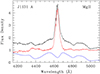 |
Fig. 1. Fe II subtraction from the Mg II blend in image A of J1131. The observed spectrum is shown in black, the Fe II spectrum in blue, and the spectrum after subtraction in red. The Fe II spectrum is the Tsuzuki et al. (2006) template convolved with the BEL width. The flux density is given in arbitrary units. |
To avoid the strong noise in the high-velocity part of μ(v), where the line flux reaches zero, it is necessary to cut the faintest parts of the line wings. We considered the parts of the line profiles whose flux density is above lcut × Fpeak, where Fpeak is the maximum flux in the line profile and lcut is fixed around 0.1. This cutoff also discards artifacts in the high-velocity wings. The resulting μ(v) profiles, binned into 20 spectral elements, are shown in Fig. 2 for the different quasars and spectral lines. The measured indices are given in Table 1. In the following, we provide details for each object.
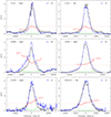 |
Fig. 2. μ(v) magnification profiles of the Mg II or Hα lines computed from simultaneously recorded spectra of two images of the quasars of our sample. The μ(v) profiles are shown in red, with the uncertainties in green. The superimposed line profiles from the microlensed image (in blue) and non-microlensed image (in black) were continuum-subtracted, corrected by the M factor, and arbitrarily rescaled. For the Mg II line profiles, the Fe II spectrum was subtracted using the Tsuzuki et al. (2006) template. The zero-velocity corresponds to the Mg IIλ2800 or Hα wavelengths at the source redshift. |
Measured magnification and distortion indices.
J1131. Sluse et al. (2007) showed that, in 2003, a clear microlensing effect was present in images A and C, while image B was unaffected. Image C being contaminated by the host galaxy light, we only considered the A, B pair. The time delay between these two images is 1.6 ± 0.7 day (Millon et al. 2020) so that the line distortions can be safely attributed to microlensing. Forbidden lines that originate in the extended narrow-line region are not affected by microlensing and the ratio of their flux measured in different images can be used to estimate the macro-magnification ratio, M. Using the [O III] λλ4959, 5007 lines, Sluse et al. (2007) found that MA/MB = 1.97 ± 0.03, while Sugai et al. (2007) measured MA/MB = 1.63 ± 0.03. We adopted the mean value, MA/MB = 1.80 ± 0.17, with an uncertainty that encompasses both values. Although the lines are fainter, a similar ratio is found from [Ne V] λλ3346, 3426: MA/MB≃ 1.85. This indicates that there is no significant wavelength-dependent differential extinction between images A and B, as was suggested by Sluse et al. (2007). We then used M(Mg II) = M(Hα) = 1.80 ± 0.17 to compute μ(v) and the indices for both the Mg II and Hα lines. The underlying continuum was measured in two windows on each side of the line profiles, [ − 33, −28] and [ + 23, +27] 103 km s−1 for Mg II and [ − 20, −17] and [ + 9, +12] 103 km s−1 for Hα, interpolated by a straight line, and subtracted from the line profiles. For both lines, we cut the faintest parts of the line profile using lcut = 0.1.
J1226. The time delay between images A and B is around 30 days (Millon et al. 2020; Donnan et al. 2021), which is short enough to suggest that the line profile distortions observed in the Mg II line are due to microlensing. A priori, either A or B can be microlensed. However, the analysis of the microlensing magnification maps computed for images A and B (Sect. 4) shows that high magnifications can be generated from the image A maps and reproduce the observations, while the equivalent strong demagnifications that would be needed for image B cannot be reached. We therefore assume that A is the microlensed image. The macro-magnification factor, MA/MB = 1.14 ± 0.10, was evaluated from the ratio of the [O II] λ3727 lines. It is in good agreement with MA/MB = 1.03 ± 0.18 measured at radio wavelengths (Jackson et al. 2024), suggesting the absence of significant wavelength-dependent differential extinction between images A and B. We then used M(Mg II) = 1.14 ± 0.10 to compute μ(v) and the indices. The continuum windows on each side of the Mg II line profile were [ − 17, −15] and [ + 11, +12] 103 km s−1. The faintest parts of the line profile were cut using lcut = 0.05.
J1355. The distortions of the Mg II line profile observed in 2005 (Sluse et al. 2012a) were still observed in 2008 (Rojas et al. 2020), and hence over a period of time much longer than the time delay between images A and B, which is around 60 days (Millon et al. 2020; Donnan et al. 2021). This confirms the microlensing interpretation, and either A or B can be microlensed. As there is no information on which image is microlensed, we have assumed that image A is microlensed (see Sect. 5.3 for further discussion). Using the macro-micro decomposition (MmD) method, Sluse et al. (2012a) measured MA/MB = 2.95 ± 0.25 at the wavelength of Mg II. The MmD provides a direct measurement of M that contains both the true macro-magnification ratio and the differential extinction. Since the value derived for Mg II was found to be in excellent agreement with the [Ne V] λλ3346, 3426 line ratio measured from images A and B (Sluse et al. 2012a), we adopted M(Mg II) = 2.95 ± 0.25 to compute μ(v) and the indices. The continuum windows on each side of the Mg II line profile were [ − 14, −10] and [ + 8, +10] 103 km s−1, avoiding the atmospheric absorption at 11 × 103 km s−1. The faintest parts of the line profile were cut using lcut = 0.075.
J1339. Image B is strongly affected by microlensing, with clear line profile distortions with respect to image A (Goicoechea & Shalyapin 2016; Shalyapin et al. 2021). The distortions are observed over a period of at least a few years, much longer than the time delay of 47 days between the two images (Shalyapin et al. 2021), which supports the microlensing interpretation. The determination of the macro-magnification factor, MB/MA = 0.20 ± 0.03, from the [O III] line ratio is discussed in Hutsemékers et al. (2024). In this object, the extinction of image A must be taken into account (Goicoechea & Shalyapin 2016; Shalyapin et al. 2021). Interpolating ϵA at the wavelength of Mg II, as was done for C IV (Hutsemékers et al. 2024), we derived M(Mg II) = 0.26 ± 0.04, which was used in the computation of μ(v) and the indices. The μ(v) profile was taken as rather narrow in velocity to avoid the strong noise that affects the red wing of the Mg II line. The continuum windows on each side of the Mg II line profile were [ − 15.5, −13.5] and [ + 25.0, +27.5] 103 km s−1. The faintest parts of the line profile were cut using lcut = 0.17.
HE0435. In this quadruply imaged quasar, image D was found microlensed and image B unaffected by microlensing (Braibant et al. 2014). The short delay between these two images of about 5 days (Millon et al. 2020; Donnan et al. 2021) supports the microlensing interpretation. The microlensing analysis previously reported in Hutsemékers et al. (2019) is revised here, based on the updated method (the use of μ(v) and not only the four indices), and a different value of M(Hα). In Braibant et al. (2014), M(Hα) = 0.47 ± 0.03 was determined with the MmD method, and used in Hutsemékers et al. (2019). However, this method can give inaccurate values if parts of the line profile are magnified and other parts are demagnified (Hutsemékers et al. 2010, 2024). After the Braibant et al. (2014) paper, Nierenberg et al. (2017) measured MD/MB = 0.67 ± 0.05 from the [O III] line ratio, in excellent agreement with MD/MB = 0.61 ± 0.09 derived from radio observations (Jackson et al. 2015). This agreement indicates the absence of significant differential extinction at the wavelength of Hα. We then adopted M(Hα) = 0.67 ± 0.05. With this value, μ(v) shows magnification of the red part of the line profile and demagnification of the blue part. The continuum windows on each side of the Hα line profile were [ − 20, −17] and [ + 8, +9] 103 km s−1. The faintest parts of the line profile were cut using lcut = 0.16.
The μ(v) magnification profiles shown in Fig. 2 have an S/N between 5 (line wings) and 25 (line core), except for J1339 where the S/N is a factor of two lower. Together with those obtained in Q2237+0305, J1004+4112, and J1138+0314 (Hutsemékers & Sluse 2021; Hutsemékers et al. 2023, 2024), the μ(v) magnification profiles show a large diversity. While the line core is often less magnified, the blue and red wings can either both be magnified, both be demagnified, or one can be magnified and the other one demagnified, or they can simply be unaffected. In a given object, the μ(v) profiles of different lines have roughly similar shapes, although the high-ionization C IV profiles show stronger magnifications than the low-ionization Mg II and Hα lines (cf. J1339 and Q2237+0305).
4. Microlensing simulations
We computed the effect of gravitational microlensing on the BEL profiles by convolving, in the source plane, the emission from BLR models with microlensing magnification maps. The microlensing simulations and the comparison to observations were carried out in the manner described in Hutsemékers et al. (2023, 2024). The method is essentially based on Braibant et al. (2017), in which the models are detailed, and Hutsemékers et al. (2019), in which the probabilistic analysis was developed.
For the BLR models, we considered a rotating Keplerian disk (KD), a biconical, radially accelerated polar wind (PW), and a radially accelerated equatorial wind (EW), with inclinations with respect to the line of sight of i = 22°, 34°, 44°, and 62°. Using the radiative transfer code STOKES (Goosmann & Gaskell 2007; Marin et al. 2012; Goosmann et al. 2014), we generated 20 BLR monochromatic images, which correspond to 20 spectral bins in the line profile. The BLR models have an emissivity of ε = ε0 (rin/r)q, where rin is the BLR inner radius of the model, and q = 3 or q = 1.5. We considered a range of rin expressed in terms of the microlensing Einstein radius in the source plane, rE. For a lens of mass ℳ,
 (2)
(2)
where DS, DL, and DLS are the source, lens, and lens-source angular diameter distances, respectively. We used between 14 and 18 values of rin, from 0.01 to 4 rE depending of the object. In all cases, the outer radius of the BLR was fixed to rout = 10 rin. The continuum source was modeled as a disk of constant surface brightness (uniform disk), with the same inclination as the BLR, and with outer radii ranging from rs= 0.02 to 5 rE.
Macro-model parameters of the lensed images.
Each microlensing simulation is based on a macro-model of the lensing galaxy that reproduces the main strong lensing observables of each system. This macro-model enabled us to predict the convergence, κ (i.e., the normalized mass surface density), and shear, γ, at the positions of the lensed images. The fraction of the local convergence in the form of stars, κ⋆/κ, is based on realistic priors. For each lensed image, we thus have a set of three parameters (κ, γ, κ⋆), which we used to compute the magnification maps. This last step was performed using the ray-tracing code developed by Wambsganss (1999). The parameters of the lensed images are given in Table 2. For all systems but J1339, the macro-model consists of an isothermal model+external shear. For J1339, Shalyapin et al. (2021) presented an ensemble of ten lens models constituted of the sum of a stellar and a dark matter component embedded into an external shear field. These ten models overfit the data but self-consistently predict the stellar fraction, κ⋆/κ, at the image positions. We elected two models that bound the expected fraction of total stellar mass in elliptical galaxies (e.g., Shajib et al. 2022). Specifically, we chose a model with a stellar fraction of κ⋆/κ = 0.11 and a model with κ⋆/κ = 0.52. For the other systems, we simply used κ⋆/κ = 0.07 and 0.21. These bounds match the constraints on the mean local stellar mass fraction derived from X-ray microlensing studies of lensed quasars (Pooley et al. 2012; Jiménez-Vicente et al. 2015). For J1131, we chose κ⋆/κ = 0.3 as an upper bound based on the analysis of the microlensing in this system by Dai et al. (2010). As is explained hereafter, our results depend weakly on κ⋆/κ, provided that it remains within the selected bounds.
To investigate the impact of the orientation of the symmetry axis of the BLR models relative to the caustic network, the maps were rotated clockwise by θ = 15°, 30°, 45°, 60°, 75°, and 90° with respect to the BLR model axis. θ = 0° corresponds to the caustic elongation and shear direction perpendicular to the BLR model axis. The final maps extend over a 100rE × 100rE area of the source plane and are sampled by 10 000 × 10 000 pixels.
Distorted line profiles were computed by convolving, for a given BLR size, the magnification maps with the monochromatic (isovelocity) images of the BLR. Simulated μ(v) profiles were then obtained for each position of the BLR on the magnification maps. The continuum-emitting region was similarly convolved. The likelihood that the simulations reproduce the observables, μcont, and the 20 spectral elements of μ(v), was finally computed for each set of parameters.
Probabilities of the Mg II and Hα BLR models.
5. Results
Examples of simulated μ(v) profiles that fit the observed μ(v) profiles are shown in Fig. 3. As has already been noticed for the C IV emission line (Hutsemékers et al. 2023; Savić et al. 2024; Hutsemékers et al. 2024), μ(v) profiles of various shapes can be reproduced by the microlensing-induced distortions of line profiles generated in the framework of the simple KD and EW models considered here. We stress that, in several cases, the observed line profile distortions can be simulated using either the KD or EW models, depending on the orientation of the magnification map with respect to the BLR model axis. As was first discussed in the case of J1004+4112 (Hutsemékers et al. 2023), this shows that the μ(v) microlensing magnification profiles strongly depend on the position of the isovelocity parts of a BLR model with respect to the caustic network, and not only on their different effective sizes, as is often assumed (for a more detailed discussion of the latter point, see Appendix A).
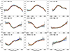 |
Fig. 3. Examples of 20 simulated μ(v) profiles (in color) that fit the μ(v) magnification profiles (in black) of the Mg II or Hα emission lines observed in J1131, J1226, J1355, J1339, and HE0435. The observed μ(v) profiles can be slightly different from those shown in Fig. 2 due to their resampling on the simulated profile velocity grid. The models are either EW or KD. The magnification maps with the smallest κ⋆/κ value were used. The maps are oriented at θ = 60° for EW models and θ = 0° for KD models, except for HE0435, where θ = 60° for KD and θ = 0° for EW (Table 3). In all models, i = 34°, q = 1.5, and rin = 0.1 rE. |
5.1. Most likely broad-line region models
The relative probability of the different models was obtained by marginalizing the likelihood over all parameters except the model and its inclination (for details, see Hutsemékers et al. 2019, 2023). The probabilities are given in Table 3 for θ ≤ 30° and θ ≥ 60° separately. Since the preferred models are found to be essentially independent of the fraction of compact matter, the probabilities computed with the different maps were merged.
For J1131, the most likely model for both the Mg II and Hα BLRs is either KD or EW, depending on the map orientation relative to the BLR axis. For J1226, we see the same dependence of the most likely model on the map orientation. For the Mg II BLR in J1355 and J1339, the EW model is preferred whatever the map orientation. The same result was obtained for the J1339 C IV BLR (Hutsemékers et al. 2024). We note that for the quasar Q2237+0305, the KD model is the most likely, whatever the orientation of the map (Savić et al. 2024). For the Hα BLR in HE0435, either KD or EW dominates, depending on the map orientation. For all objects, the PW model has a lower probability. The inclination, i, is poorly constrained, but it is smaller than 45°, as is expected for type 1 quasars. As for the high-ionization C IV BLR, we can conclude that disk geometries with kinematics dominated by either Keplerian rotation or equatorial outflow best reproduce the microlensing effects on the low-ionization Mg II and Hα emission line profiles. We emphasize that the KD and EW models could be discriminated if we had knowledge of the orientation of the BLR axis on the sky, such as the one given by the orientation of the radio jet.
5.2. Size of the broad emission line region
We estimated the most likely BLR radius by marginalizing over all parameters but rin. From the rin distribution, we computed the half-light radius, r1/2, and flux-weighted mean radius, rmean, distributions, following Hutsemékers & Sluse (2021). Figure 4 shows the posterior probability densities, uniformly resampled on a logarithmic scale, of the BLR radii, r1/2 and rmean, for the different objects and lines. The results obtained with different values of the fraction of compact objects, κ⋆/κ, are illustrated separately. The probability distributions do not significantly depend on κ⋆/κ. The largest difference is observed for the Mg II BLR radius in J1131, but the distributions still largely overlap.
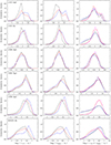 |
Fig. 4. Posterior probability densities of the radius of the Mg II or Hα BLR. The BLR radius is expressed in Einstein radius units. It was computed with ℳ = 0.3 ℳ⊙, rE = 9.7, 9.2, 8.1, 10.1, 11.5 light-days for J1131, J1226, J1355, J1339, and HE0435, respectively. Left panels: Probability densities of the half-light radius, r1/2, obtained with two magnification maps characterized by low (black) and high (blue) fractions of compact objects, and after marginalizing over the two maps (red). Middle panels: Same as the left panels but for the flux-weighted mean radius, rmean. Right panels: Comparison of the probability densities, marginalized over the two maps, of the half-light radius (red and blue curves) and the flux-weighted mean radius (magenta and black curves), computed with constraints from the continuum source magnification (red and magenta curves) and without this constraint (blue and black curves). |
Our microlensing simulations simultaneously fit the magnification profile, μ(v), and the continuum magnification, μcont (Sect. 4). We also show, in the right panels of Fig. 4, the probability distributions computed by only taking into account the μ(v) profile (which necessitates much less computing time). In most cases, the probability distributions are in excellent agreement, indicating that taking into account μcont does not improve the constraints on the BLR size. This can be explained by the fact that the BLR covers a larger area of the magnification map than the continuum source.
Table 4 gives the BLR radii, computed from the median values of the probability distributions shown in Fig. 4. The uncertainties correspond to the equal-tailed credible intervals that enclose a posterior probability of 68%. The radii and intervals are then converted to a linear scale, multiplied by rE, and expressed in light-days. To compute the Einstein radius (Eq. 2), we adopted a flat lambda cold dark matter (ΛCDM) cosmology with H0 = 68 km s−1 Mpc−1 and Ωm = 0.31. We derived rE = 9.7, 9.2, 8.1, 10.1, 11.5  light-days for J1131, J1226, J1355, J1339, and HE0435, respectively. ℳ⊙ is the solar mass.
BLR radii.
For a given quasar line, all of the BLR radii agree within the uncertainties. We found no significant difference between r1/2 and rmean, or between measurements with and without the constraint from μcont. For J1131, we found no difference between the Mg II and Hα BLR radii. On the other hand, the Mg II BLR radius in J1339 is about a factor of four larger than the radius of the C IV BLR measured by Hutsemékers et al. (2024). This is in agreement with the difference between the low- and high-ionization BLR radii reported by Guerras et al. (2013) and Fian et al. (2021).
5.3. Radius-luminosity relations
The R − L relation for the Mg II BLR is illustrated in Fig. 5. It shows the reverberation mapping measurements of Yu et al. (2023) and Shen et al. (2024), together with our measurements from microlensing (the “All maps” half-light radii reported in Table 4). We added the Mg II BLR sizes independently obtained for Q0957+561 and J1004+4112 by Fian et al. (2023, 2024a). The R − L relation for the Hα BLR is illustrated in Fig. 6. It includes the reverberation mapping measurements obtained for the Hα BLR by Shen et al. (2024). Since these data cover a limited luminosity range, we also showed the measurements of Bentz et al. (2013) for the Hβ BLR, without any correction but keeping in mind that the Hβ BLR could be smaller than the Hα BLR by about 0.15 dex (Grier et al. 2017). To the microlensing BLR radii obtained for J1131 and HE0435, we added the Hα BLR radius of Q2237+0305 given in Savić et al. (2024). The macro-magnification-corrected luminosities are reported in Table 5 for the five systems for which we derived a BLR size and for the three systems with measurements from literature; that is, Q0957+561, J1004+4112, and Q2237+0305. When the monochromatic luminosities were not available for a wavelength of interest (i.e., 3000 Å), we applied the bolometric correction ratios from Sluse et al. (2012a) to convert published monochromatic luminosities to λLλ (3000 Å). For Q0957+561, we used λLλ (5100 Å) from Guerras et al. (2013) and assumed an uncertainty of 0.1 dex. For J1004+4112, we used λLλ (1350 Å) from Hutsemékers et al. (2023).
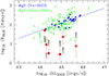 |
Fig. 5. Radius-luminosity relation for the Mg II BLR. The rest-frame time lag from reverberation mapping and the continuum luminosity at 3000 Å are from Yu et al. (2023, in blue) and Shen et al. (2024, in green). The fit from Yu et al. (2023) is superimposed as a continuous line. The BLR half-light radii measured from microlensing are superimposed in red. Squares show the measurements from this work. Diamonds show the measurements from Fian et al. (2023); Fian et al. (2024a) for Q0957+561 and J1004+4112. |
Magnification-corrected monochromatic luminosities.
We immediately see from Figs. 5 and 6 that, except for Q0957+561, the BLR radii derived from microlensing are systematically below the R − L relations obtained with reverberation mapping. For the Mg II BLR, the deviation is particularly strong, reaching a factor of 30 for J1226. A smaller deviation was already suspected for the C IVR − L relation (Hutsemékers et al. 2024).
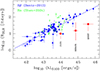 |
Fig. 6. Radius–luminosity relation for the Hα and Hβ BLRs. The rest-frame time lag from reverberation mapping and the continuum luminosity at 5100 Å are from Bentz et al. (2013, Hβ measurements, in blue) and Shen et al. (2024, Hα measurements, in green). The fit from Bentz et al. (2013) is superimposed as a continuous line. The Hα BLR half-light radii measured from microlensing are superimposed as red squares. |
As was shown in the previous section, the microlensing BLR radii are robust, within uncertainties, with respect to changes in the magnification map, in particular the stellar mass fraction, and to changes in the radius calculation, either half-light or flux-weighted. As is discussed in Hutsemékers et al. (2024), the microlensing BLR radius is sensitive to the macro-magnification factor used in the computation of μ(v). For J1226, we then considered a higher, but still reasonable value: M = 1.4 ± 0.1 such that μ(v = 0)≃1. With this value, we obtained r1/2 =  light-days instead of 2.9
 light-days, which is slightly higher and within the uncertainties, but still far from a factor of 30. We also computed μ(v) as the ratio of the magnification profiles produced with maps specific to images A and B, and thus have assumed a significant microlensing effect in image B. We found r1/2 =
  light-days, which is again in good agreement with the values reported in Table 4. The same exercise with J1355 leads to r1/2 =
  light-days, which is equal, within the uncertainties, to the value given in Table 4. Finally, a change in the average stellar mass, ℳ = 0.3 ℳ⊙, could in principle increase r1/2 but it would require an average stellar mass that is almost three orders of magnitude larger to explain a factor of 30, which is unrealistic (Poindexter & Kochanek 2010; Jiménez-Vicente & Mediavilla 2019).
Based on a dense spectroscopic monitoring secured between 2008 and 2011 (about 150 spectra), we were able to estimate the size of the BLR in J1131 with the reverberation mapping technique (Sluse et al., in prep.). Using two different methods for measuring the time lag between the R-band continuum and the Hβ emission, a BLR radius of about 15 light-days was obtained, with an uncertainty of around 30%. Hence, the reverberation mapping radius is in agreement, within the uncertainties, with the BLR size estimated from single-epoch microlensing (Table 4). Both techniques, microlensing and reverberation mapping2, thus give a BLR size for J1131 below the R − L relation. While the measurement of the BLR size using both microlensing and reverberation mapping is only available for one object, this result further supports the reliability of the microlensing method in estimating BLR sizes.
Our measurements thus confirm that the intrinsic dispersion of the BLR radii with respect to the R − L relation is large, as has already been shown by Shen et al. (2024). However, the fact that the microlensing BLR radii are systematically below the R − L relations remains to be explained.
In Fig. 7, we show the distribution of the microlensing BLR radii expressed in Einstein radii, for the quasars studied so far. The BLR radius is comparable to the Einstein radius within roughly a factor of two (0.3 dex). This can be expected, since a very small BLR with respect to the Einstein radius would be entirely magnified, with no line profile distortion, while a much larger BLR would be totally unaffected. This distribution is the result of our selection of lensed quasars that show line profile distortions. In Fig. 8, assuming RBLR ≃ rE, we plotted the microlensing Einstein radius of lensed quasars against the quasar luminosity using the sample compiled by Mosquera & Kochanek (2011). The luminosities at 5100 Å were computed back using the BLR radius and the R − L relation given in that paper. With these luminosities and the bolometric corrections from Sluse et al. (2012a), we derived the luminosities at 1350 Å and 3000 Å, from which we computed the R − L relations for Hβ (Bentz et al. 2013), Mg II (Yu et al. 2023), and C IV (Kaspi et al. 2021), as a function of the 5100 Å luminosity. These relations are shown in Fig. 8.
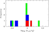 |
Fig. 7. Distribution of the BLR half-light radii derived from our microlensing analysis, expressed in units of rE. The Mg II and Hα BLR radii from this work are represented in green and red, respectively, and the C IV BLR radii from Hutsemékers et al. (2023, 2024) and Savić et al. (2024) in blue. |
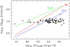 |
Fig. 8. BLR radius – quasar luminosity relations shown as a function of the luminosity at 5100 Å (continuous lines) for the C IV (Kaspi et al. 2021, in blue), Mg II (Yu et al. 2023, in green), and Hβ (Bentz et al. 2013, in red) BLRs. The microlensing Einstein radii of lensed quasars from the compilation of Mosquera & Kochanek (2011) are superimposed (black diamonds). |
If we pick objects with observed line profile distortions, and hence RBLR ≃ rE, we see that the BLR radii of high-luminosity (log[λLλ (5100 Å)] ≳ 44) quasars are below the R − L relations. The selection effect appears stronger for Mg II, intermediate for Hα, and smaller for C IV, in agreement with the deviations observed in Figs. 5 and 6, and in Fig. 8 of Hutsemékers et al. (2024), where the average deviations are measured to be 1.0, 0.64, and 0.48 dex, for Mg II, Hα, and C IV, respectively. This selection bias appears because the microlensing Einstein radii of currently detected lensed quasars are strongly concentrated around a single value, about ten light-days for an average microlens mass of 0.3 ℳ⊙. As can be calculated from Eq. (2), this follows from the fact that the lens redshift distribution peaks around zl ≃ 0.5 − 1.0 for lensed quasars at zs ≃ 2 (e.g., Ofek et al. 2003).
The fact that the microlensing BLR radii are systematically below the R − L relations is thus a selection effect. Since the selection bias depends on the line under study, it should also be taken into account when comparing, on a statistical basis, the sizes of the regions that emit different lines. In particular, the difference between the averaged Mg II and C IV BLR sizes would be underestimated if selection bias corrections were not applied.
6. Summary and conclusions
We have analyzed the microlensing-induced line profile distortions observed in Mg II and/or Hα in five gravitationally lensed quasars, J1131-1231, J1226-0006, J1355-2257, J1339+1310, and HE0435-1223, using single-epoch spectroscopic data. This study complements our previous analyses of the C IV high-ionization line distortions observed in four lensed quasars, Q2237+0305, J1004+4112, J1339+1310, and J1138+0314 (Hutsemékers & Sluse 2021; Hutsemékers et al. 2023, 2024; Savić et al. 2024). We first noticed that there are a wide variety of μ(v) magnification profiles. While the line core is often less magnified, the blue and red wings can either both be magnified, both be demagnified, or one can be magnified and the other one demagnified, or they can simply be unaffected. For a given object, the μ(v) profiles of different lines have roughly similar shapes, although the high-ionization line profiles tend to show stronger magnifications than the low-ionization ones.
To characterize the size, geometry, and kinematics of the BLR, we have compared the observed line profile distortions with simulated ones. The simulations are based on three BLR models (KD, EW, and PW) of different sizes, inclinations, and emissivities, convolved with microlensing magnification maps specific to the microlensed quasar images. We found that:
-
The observed line profile distortions can all be reproduced with microlensing-induced distortions of line profiles generated from our simple BLR models. In several cases, the observed distortions can be simulated using either the KD or EW models, depending on the orientation of the magnification map with respect to the BLR axis. This demonstrates that the μ(v) magnification profiles depend on the position and orientation of the isovelocity parts of a BLR model with respect to the caustic network, and not only on their different effective sizes.
-
For J1131, J1226, and HE0435, the most likely model for the Mg II and Hα BLRs is either KD or EW, depending on the map orientation relative to the BLR axis. For the Mg II BLR in J1355 and J1339, the EW model is preferred. For all objects, the PW model has a lower probability. The inclination is poorly constrained, but it is smaller than 45°, as is expected for type 1 quasars. As for the high-ionization C IV BLR, we can conclude that disk geometries with kinematics dominated by either Keplerian rotation or equatorial outflow best reproduce the microlensing effects on the low-ionization Mg II and Hα emission line profiles.
-
The half-light radii of the Mg II and Hα BLRs were measured in the range of 3 to 25 light-days. In J1131, the Mg II and Hα BLRs have the same radius. In J1339, the Mg II BLR radius is about a factor of four larger than the radius of the C IV BLR. The measured BLR radii are robust, within uncertainties, to changes in the magnification map, in particular the stellar mass fraction, and to changes in the radius calculation. For J1131, the BLR radius derived from reverberation mapping is in agreement with the microlensing BLR radius within the uncertainties.
-
The microlensing BLR radii of the Mg II and Hα BLRs were compared with R − L relations derived from reverberation mapping, and found to be systematically below. For the Mg II BLR, the deviation is particularly strong, reaching a factor of 30 for J1226. This confirms that the intrinsic dispersion of the BLR radii with respect to the R − L relations is large. This also reveals a strong selection bias that affects microlensing-based BLR size measurements. This bias arises from the fact that, if microlensing-induced line profile distortions are observed in a lensed quasar, the BLR radius should be comparable to the Einstein radius, which clusters in a narrow range of values regardless of the (realistic) redshifts of the lens and the source.
It should be kept in mind that, in some cases, the response-weighted time delay measured with reverberation mapping could differ from the flux-weighted radius by up to a factor of two (Rosborough et al. 2024).
Acknowledgments
D.H. and Đ.S. acknowledge support from the Fonds de la Recherche Scientifique – FNRS (Belgium) under grants PDR T.0116.21 and No 4.4503.19.
References
- Abajas, C., Mediavilla, E., Muñoz, J. A., Popović, L. Č., & Oscoz, A. 2002, ApJ, 576, 640 [Google Scholar]
- Abajas, C., Mediavilla, E., Muñoz, J. A., Gómez-Álvarez, P., & Gil-Merino, R. 2007, ApJ, 658, 748 [CrossRef] [Google Scholar]
- Assef, R. J., Denney, K. D., Kochanek, C. S., et al. 2011, ApJ, 742, 93 [Google Scholar]
- Bentz, M. C., Denney, K. D., Grier, C. J., et al. 2013, ApJ, 767, 149 [Google Scholar]
- Braibant, L., Hutsemékers, D., Sluse, D., Anguita, T., & García-Vergara, C. J. 2014, A&A, 565, L11 [NASA ADS] [CrossRef] [EDP Sciences] [Google Scholar]
- Braibant, L., Hutsemékers, D., Sluse, D., & Anguita, T. 2016, A&A, 592, A23 [NASA ADS] [CrossRef] [EDP Sciences] [Google Scholar]
- Braibant, L., Hutsemékers, D., Sluse, D., & Goosmann, R. 2017, A&A, 607, A32 [NASA ADS] [CrossRef] [EDP Sciences] [Google Scholar]
- Dai, X., Kochanek, C. S., Chartas, G., et al. 2010, ApJ, 709, 278 [Google Scholar]
- Donnan, F. R., Horne, K., & Hernández Santisteban, J. V. 2021, MNRAS, 508, 5449 [NASA ADS] [CrossRef] [Google Scholar]
- Eigenbrod, A., Courbin, F., Meylan, G., Vuissoz, C., & Magain, P. 2006, A&A, 451, 759 [NASA ADS] [CrossRef] [EDP Sciences] [Google Scholar]
- Fian, C., Guerras, E., Mediavilla, E., et al. 2018, ApJ, 859, 50 [Google Scholar]
- Fian, C., Mediavilla, E., Motta, V., et al. 2021, A&A, 653, A109 [NASA ADS] [CrossRef] [EDP Sciences] [Google Scholar]
- Fian, C., Muñoz, J. A., Mediavilla, E., et al. 2023, A&A, 678, A108 [NASA ADS] [CrossRef] [EDP Sciences] [Google Scholar]
- Fian, C., Muñoz, J. A., Forés-Toribio, R., et al. 2024a, A&A, 682, A57 [NASA ADS] [CrossRef] [EDP Sciences] [Google Scholar]
- Fian, C., Jiménez-Vicente, J., Mediavilla, E., et al. 2024b, ApJ, 972, L7 [NASA ADS] [CrossRef] [Google Scholar]
- Garsden, H., Bate, N. F., & Lewis, G. F. 2011, MNRAS, 418, 1012 [NASA ADS] [CrossRef] [Google Scholar]
- Gil-Merino, R., Goicoechea, L. J., Shalyapin, V. N., & Oscoz, A. 2018, A&A, 616, A118 [NASA ADS] [CrossRef] [EDP Sciences] [Google Scholar]
- Goicoechea, L. J., & Shalyapin, V. N. 2016, A&A, 596, A77 [NASA ADS] [CrossRef] [EDP Sciences] [Google Scholar]
- Goosmann, R. W., & Gaskell, C. M. 2007, A&A, 465, 129 [NASA ADS] [CrossRef] [EDP Sciences] [Google Scholar]
- Goosmann, R. W., Gaskell, C. M., & Marin, F. 2014, Adv. Space Res., 54, 1341 [NASA ADS] [CrossRef] [Google Scholar]
- Grier, C. J., Trump, J. R., Shen, Y., et al. 2017, ApJ, 851, 21 [NASA ADS] [CrossRef] [Google Scholar]
- Guerras, E., Mediavilla, E., Jimenez-Vicente, J., et al. 2013, ApJ, 764, 160 [Google Scholar]
- Hutsemékers, D., & Sluse, D. 2021, A&A, 654, A155 [NASA ADS] [CrossRef] [EDP Sciences] [Google Scholar]
- Hutsemékers, D., Borguet, B., Sluse, D., Riaud, P., & Anguita, T. 2010, A&A, 519, A103 [NASA ADS] [CrossRef] [EDP Sciences] [Google Scholar]
- Hutsemékers, D., Braibant, L., Sluse, D., & Goosmann, R. 2019, A&A, 629, A43 [NASA ADS] [CrossRef] [EDP Sciences] [Google Scholar]
- Hutsemékers, D., Sluse, D., Savić, Đ., & Richards, G. T. 2023, A&A, 672, A45 [NASA ADS] [CrossRef] [EDP Sciences] [Google Scholar]
- Hutsemékers, D., Sluse, D., & Savić, Đ. 2024, A&A, 687, A153 [NASA ADS] [CrossRef] [EDP Sciences] [Google Scholar]
- Inada, N., Oguri, M., Becker, R. H., et al. 2008, AJ, 135, 496 [NASA ADS] [CrossRef] [Google Scholar]
- Jackson, N., Tagore, A. S., Roberts, C., et al. 2015, MNRAS, 454, 287 [Google Scholar]
- Jackson, N., Badole, S., Dugdale, T., et al. 2024, MNRAS, 530, 221 [NASA ADS] [CrossRef] [Google Scholar]
- Jiménez-Vicente, J., & Mediavilla, E. 2019, ApJ, 885, 75 [Google Scholar]
- Jiménez-Vicente, J., Mediavilla, E., Kochanek, C. S., & Muñoz, J. A. 2015, ApJ, 799, 149 [Google Scholar]
- Kaspi, S., Brandt, W. N., Maoz, D., et al. 2021, ApJ, 915, 129 [NASA ADS] [CrossRef] [Google Scholar]
- Keeton, C. R., Burles, S., Schechter, P. L., & Wambsganss, J. 2006, ApJ, 639, 1 [CrossRef] [Google Scholar]
- Lewis, G. F., & Ibata, R. A. 2004, MNRAS, 348, 24 [NASA ADS] [CrossRef] [Google Scholar]
- Marin, F., Goosmann, R. W., Gaskell, C. M., Porquet, D., & Dovčiak, M. 2012, A&A, 548, A121 [NASA ADS] [CrossRef] [EDP Sciences] [Google Scholar]
- Metcalf, R. B., Moustakas, L. A., Bunker, A. J., & Parry, I. R. 2004, ApJ, 607, 43 [NASA ADS] [CrossRef] [Google Scholar]
- Millon, M., Courbin, F., Bonvin, V., et al. 2020, A&A, 640, A105 [NASA ADS] [CrossRef] [EDP Sciences] [Google Scholar]
- Morgan, N. D., Gregg, M. D., Wisotzki, L., et al. 2003, AJ, 126, 696 [NASA ADS] [CrossRef] [Google Scholar]
- Mortonson, M. J., Schechter, P. L., & Wambsganss, J. 2005, ApJ, 628, 594 [NASA ADS] [CrossRef] [Google Scholar]
- Mosquera, A. M., & Kochanek, C. S. 2011, ApJ, 738, 96 [Google Scholar]
- Motta, V., Mediavilla, E., Rojas, K., et al. 2017, ApJ, 835, 132 [NASA ADS] [CrossRef] [Google Scholar]
- Nemiroff, R. J. 1988, ApJ, 335, 593 [NASA ADS] [CrossRef] [Google Scholar]
- Nierenberg, A. M., Treu, T., Brammer, G., et al. 2017, MNRAS, 471, 2224 [NASA ADS] [CrossRef] [Google Scholar]
- O’Dowd, M., Bate, N. F., Webster, R. L., Wayth, R., & Labrie, K. 2011, MNRAS, 415, 1985 [CrossRef] [Google Scholar]
- Ofek, E. O., Rix, H.-W., & Maoz, D. 2003, MNRAS, 343, 639 [NASA ADS] [CrossRef] [Google Scholar]
- Poindexter, S., & Kochanek, C. S. 2010, ApJ, 712, 658 [NASA ADS] [CrossRef] [Google Scholar]
- Pooley, D., Rappaport, S., Blackburne, J. A., Schechter, P. L., & Wambsganss, J. 2012, ApJ, 744, 111 [NASA ADS] [CrossRef] [Google Scholar]
- Popović, L. Č., Mediavilla, E. G., & Muñoz, J. A. 2001, A&A, 378, 295 [NASA ADS] [CrossRef] [EDP Sciences] [Google Scholar]
- Popović, L. Č., Afanasiev, V. L., Moiseev, A., et al. 2020, A&A, 634, A27 [EDP Sciences] [Google Scholar]
- Richards, G. T., Keeton, C. R., Pindor, B., et al. 2004, ApJ, 610, 679 [NASA ADS] [CrossRef] [Google Scholar]
- Rojas, K., Motta, V., Mediavilla, E., et al. 2020, ApJ, 890, 3 [Google Scholar]
- Rosborough, S. A., Robinson, A., Almeyda, T., & Noll, M. 2024, ApJ, 965, 35 [NASA ADS] [CrossRef] [Google Scholar]
- Savić, Đ., Hutsemékers, D., & Sluse, D. 2024, A&A, 687, A114 [NASA ADS] [CrossRef] [EDP Sciences] [Google Scholar]
- Schneider, P., & Wambsganss, J. 1990, A&A, 237, 42 [NASA ADS] [Google Scholar]
- Shajib, A. J., Vernardos, G., Collett, T. E., et al. 2022, arXiv e-prints [arXiv:2210.10790] [Google Scholar]
- Shalyapin, V. N., & Goicoechea, L. J. 2014, A&A, 568, A116 [NASA ADS] [CrossRef] [EDP Sciences] [Google Scholar]
- Shalyapin, V. N., Goicoechea, L. J., Morgan, C. W., Cornachione, M. A., & Sergeyev, A. V. 2021, A&A, 646, A165 [NASA ADS] [CrossRef] [EDP Sciences] [Google Scholar]
- Shen, Y., Grier, C. J., Horne, K., et al. 2024, ApJS, 272, 26 [NASA ADS] [CrossRef] [Google Scholar]
- Simić, S., & Popović, L. Č. 2014, Adv. Space Res., 54, 1439 [CrossRef] [Google Scholar]
- Sluse, D., Surdej, J., Claeskens, J. F., et al. 2003, A&A, 406, L43 [NASA ADS] [CrossRef] [EDP Sciences] [Google Scholar]
- Sluse, D., Claeskens, J.-F., Hutsemékers, D., & Surdej, J. 2007, A&A, 468, 885 [NASA ADS] [CrossRef] [EDP Sciences] [Google Scholar]
- Sluse, D., Schmidt, R., Courbin, F., et al. 2011, A&A, 528, A100 [NASA ADS] [CrossRef] [EDP Sciences] [Google Scholar]
- Sluse, D., Hutsemékers, D., Courbin, F., Meylan, G., & Wambsganss, J. 2012a, A&A, 544, A62 [NASA ADS] [CrossRef] [EDP Sciences] [Google Scholar]
- Sluse, D., Chantry, V., Magain, P., Courbin, F., & Meylan, G. 2012b, A&A, 538, A99 [NASA ADS] [CrossRef] [EDP Sciences] [Google Scholar]
- Sugai, H., Kawai, A., Shimono, A., et al. 2007, ApJ, 660, 1016 [NASA ADS] [CrossRef] [Google Scholar]
- Tsuzuki, Y., Kawara, K., Yoshii, Y., et al. 2006, ApJ, 650, 57 [NASA ADS] [CrossRef] [Google Scholar]
- Vestergaard, M., & Wilkes, B. J. 2001, ApJS, 134, 1 [Google Scholar]
- Wambsganss, J. 1999, J. Comput. Appl. Math., 109, 353 [NASA ADS] [CrossRef] [Google Scholar]
- Wayth, R. B., O’Dowd, M., & Webster, R. L. 2005, MNRAS, 359, 561 [NASA ADS] [CrossRef] [Google Scholar]
- Wisotzki, L., Schechter, P. L., Bradt, H. V., Heinmüller, J., & Reimers, D. 2002, A&A, 395, 17 [NASA ADS] [CrossRef] [EDP Sciences] [Google Scholar]
- Yu, Z., Martini, P., Penton, A., et al. 2023, MNRAS, 522, 4132 [NASA ADS] [CrossRef] [Google Scholar]
Appendix A: Size is not everything in BLR microlensing
Recently Fian et al. (2024b) used the Si IV and C IV magnification profiles in five lensed quasars to infer the inner BLR kinematics. They essentially showed that the magnification profiles can be reproduced with the KD kinematics, in agreement with results reported in Hutsemékers & Sluse (2021), Hutsemékers et al. (2023, 2024), and Savić et al. (2024). However, they rejected alternatives that involve radial motions, arguing that precise fine-tuning would be needed to reproduce the observed magnification profiles. On the contrary, we have shown that both the KD and EW models can reproduce the same magnification profiles with similar probabilities, depending on the orientation of the BLR axis with respect to the caustic map. This dependence on the BLR axis - magnification map relative orientation is due to the fact that in KD models the highest velocities come from regions located, in projection, perpendicular to the BLR axis, while in EW models these regions are parallel to the BLR axis (see Fig. 3 of Braibant et al. 2017). Furthermore, in the specific case of J1339+1310, we showed that the EW model reproduces the C IV magnification profile better than the KD models. Similar conclusions are reached for the low-ionization lines studied in the present paper.
The analysis of Fian et al. (2024b) is based on the hypothesis that the magnification of a velocity bin in the line profile is only determined by the size of the BLR subregion at the origin of this velocity bin. In this framework, since the observed (de)magnification is often stronger at large velocities, the size of the emitting region is assumed to decrease with increasing velocity, which can be explained by the KD kinematics. In our analysis, we do not make this assumption; the relative positions and sizes of the BLR subregions are fixed within the adopted model, and cannot be arbitrarily assigned. The emissivity law, in particular, contributes to constrain the size of the emitting regions. The location and orientation of the different BLR subregions with respect to the caustic network are then found as important as the size to reproduce the observed magnification profiles, a conclusion already reached by Abajas et al. (2007) for a biconical geometry. Without the hypothesis that only size controls the magnification, both the KD and EW models can fit the same observed magnification profiles (see Fig. 3, and Fig. 7 of Hutsemékers et al. 2023), even if the mean emission radius increases as a function of the velocity in the EW model (Fig. A.1). Note also that the mean emission radius of the KD models does not change by more than a factor of three as a function of the velocity (and by no more than about 70% for the EW model), so that size alone cannot explain the high differential magnifications observed in the BELs of some objects. In Fig. A.2 (see also Braibant et al. 2017; Hutsemékers et al. 2019; Hutsemékers & Sluse 2021, for other examples), we show an example of two-dimensional distributions of the WCI and RBI indices. These indices, that characterize line profile distortions (Sect. 3), were computed from the line profiles generated by the convolution of the KD, PW, and EW models with a magnification map. We see that a large diversity of WCI and RBI values, which encompass the observed ones, can be produced, even when considering a single BLR radius. The KD and EW models generate the strongest distortions, with comparable probabilities when combining all map orientations, and without fine-tuning. Finally, it is worth noticing that the low magnification of the line core can be simultaneously fitted with the adopted KD and EW models, without assuming that the line core originates from a much larger, independent, BLR (Fian et al. 2024b).
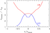 |
Fig. A.1. Flux-weighted mean radius of the BLR isovelocity slices as a function of the Doppler velocity in the line profile. The mean radius is computed for the 20 isovelocity slices of the KD and EW models, with an emissivity ε = ε0 (rin/r)3, and seen at an inclination of 34°. A more complete version can be found in Braibant et al. (2017). Using the half-radius instead of the mean radius does not change the velocity dependence. |
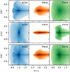 |
Fig. A.2. Two-dimensional histograms of simulated WCI and RBI (the darkest regions correspond to the highest frequencies). These indices were measured from simulated line profiles that arise from the BLR models KD, PW, and EW seen at an inclination of 34°, and with an emissivity ε = ε0 (rin/r)3. The simulations include the map orientations θ = [0°, 30°] (top panel), θ = [60°, 90°] (middle panel), and θ = [0°, 30°, 60°, 90°] (bottom panel) which is the combination of the top and middle panels. These histograms were built from the magnification maps used for the analysis of J1004+4112 (Hutsemékers et al. 2023). They show a particularly clear dependence on the map orientation. The simulations were restricted to 0.9 ≤ μBLR ≤ 1.1, and to a single value of the BLR size, rin = 0.1rE. |
To summarize, our results demonstrate that the assumption that “size is everything”, which is useful to estimate the size and wavelength dependence of the smaller continuum source (Mortonson et al. 2005), cannot be applied to infer the BLR kinematics, without arbitrarily discarding some possible models. We emphasize that our discussion refers to the microlensing of individual velocity bins, not to the estimation of the BLR size as a whole.
All Tables
All Figures
|
Fig. 1. Fe II subtraction from the Mg II blend in image A of J1131. The observed spectrum is shown in black, the Fe II spectrum in blue, and the spectrum after subtraction in red. The Fe II spectrum is the Tsuzuki et al. (2006) template convolved with the BEL width. The flux density is given in arbitrary units. |
| In the text | |
|
Fig. 2. μ(v) magnification profiles of the Mg II or Hα lines computed from simultaneously recorded spectra of two images of the quasars of our sample. The μ(v) profiles are shown in red, with the uncertainties in green. The superimposed line profiles from the microlensed image (in blue) and non-microlensed image (in black) were continuum-subtracted, corrected by the M factor, and arbitrarily rescaled. For the Mg II line profiles, the Fe II spectrum was subtracted using the Tsuzuki et al. (2006) template. The zero-velocity corresponds to the Mg IIλ2800 or Hα wavelengths at the source redshift. |
| In the text | |
|
Fig. 3. Examples of 20 simulated μ(v) profiles (in color) that fit the μ(v) magnification profiles (in black) of the Mg II or Hα emission lines observed in J1131, J1226, J1355, J1339, and HE0435. The observed μ(v) profiles can be slightly different from those shown in Fig. 2 due to their resampling on the simulated profile velocity grid. The models are either EW or KD. The magnification maps with the smallest κ⋆/κ value were used. The maps are oriented at θ = 60° for EW models and θ = 0° for KD models, except for HE0435, where θ = 60° for KD and θ = 0° for EW (Table 3). In all models, i = 34°, q = 1.5, and rin = 0.1 rE. |
| In the text | |
|
Fig. 4. Posterior probability densities of the radius of the Mg II or Hα BLR. The BLR radius is expressed in Einstein radius units. It was computed with ℳ = 0.3 ℳ⊙, rE = 9.7, 9.2, 8.1, 10.1, 11.5 light-days for J1131, J1226, J1355, J1339, and HE0435, respectively. Left panels: Probability densities of the half-light radius, r1/2, obtained with two magnification maps characterized by low (black) and high (blue) fractions of compact objects, and after marginalizing over the two maps (red). Middle panels: Same as the left panels but for the flux-weighted mean radius, rmean. Right panels: Comparison of the probability densities, marginalized over the two maps, of the half-light radius (red and blue curves) and the flux-weighted mean radius (magenta and black curves), computed with constraints from the continuum source magnification (red and magenta curves) and without this constraint (blue and black curves). |
| In the text | |
|
Fig. 5. Radius-luminosity relation for the Mg II BLR. The rest-frame time lag from reverberation mapping and the continuum luminosity at 3000 Å are from Yu et al. (2023, in blue) and Shen et al. (2024, in green). The fit from Yu et al. (2023) is superimposed as a continuous line. The BLR half-light radii measured from microlensing are superimposed in red. Squares show the measurements from this work. Diamonds show the measurements from Fian et al. (2023); Fian et al. (2024a) for Q0957+561 and J1004+4112. |
| In the text | |
|
Fig. 6. Radius–luminosity relation for the Hα and Hβ BLRs. The rest-frame time lag from reverberation mapping and the continuum luminosity at 5100 Å are from Bentz et al. (2013, Hβ measurements, in blue) and Shen et al. (2024, Hα measurements, in green). The fit from Bentz et al. (2013) is superimposed as a continuous line. The Hα BLR half-light radii measured from microlensing are superimposed as red squares. |
| In the text | |
|
Fig. 7. Distribution of the BLR half-light radii derived from our microlensing analysis, expressed in units of rE. The Mg II and Hα BLR radii from this work are represented in green and red, respectively, and the C IV BLR radii from Hutsemékers et al. (2023, 2024) and Savić et al. (2024) in blue. |
| In the text | |
|
Fig. 8. BLR radius – quasar luminosity relations shown as a function of the luminosity at 5100 Å (continuous lines) for the C IV (Kaspi et al. 2021, in blue), Mg II (Yu et al. 2023, in green), and Hβ (Bentz et al. 2013, in red) BLRs. The microlensing Einstein radii of lensed quasars from the compilation of Mosquera & Kochanek (2011) are superimposed (black diamonds). |
| In the text | |
|
Fig. A.1. Flux-weighted mean radius of the BLR isovelocity slices as a function of the Doppler velocity in the line profile. The mean radius is computed for the 20 isovelocity slices of the KD and EW models, with an emissivity ε = ε0 (rin/r)3, and seen at an inclination of 34°. A more complete version can be found in Braibant et al. (2017). Using the half-radius instead of the mean radius does not change the velocity dependence. |
| In the text | |
|
Fig. A.2. Two-dimensional histograms of simulated WCI and RBI (the darkest regions correspond to the highest frequencies). These indices were measured from simulated line profiles that arise from the BLR models KD, PW, and EW seen at an inclination of 34°, and with an emissivity ε = ε0 (rin/r)3. The simulations include the map orientations θ = [0°, 30°] (top panel), θ = [60°, 90°] (middle panel), and θ = [0°, 30°, 60°, 90°] (bottom panel) which is the combination of the top and middle panels. These histograms were built from the magnification maps used for the analysis of J1004+4112 (Hutsemékers et al. 2023). They show a particularly clear dependence on the map orientation. The simulations were restricted to 0.9 ≤ μBLR ≤ 1.1, and to a single value of the BLR size, rin = 0.1rE. |
| In the text | |
Current usage metrics show cumulative count of Article Views (full-text article views including HTML views, PDF and ePub downloads, according to the available data) and Abstracts Views on Vision4Press platform.
Data correspond to usage on the plateform after 2015. The current usage metrics is available 48-96 hours after online publication and is updated daily on week days.
Initial download of the metrics may take a while.