| Issue |
A&A
Volume 646, February 2021
|
|
|---|---|---|
| Article Number | A133 | |
| Number of page(s) | 20 | |
| Section | Stellar structure and evolution | |
| DOI | https://doi.org/10.1051/0004-6361/202039532 | |
| Published online | 18 February 2021 | |
Calibrating core overshooting parameters with two-dimensional hydrodynamical simulations
1
Max-Planck-Institut für Astrophysik, Karl-Schwarzschild-Str. 1, 85748 Garching, Germany
2
Technische Universität München, Physik Department, James Franck Str. 1, 85748 Garching, Germany
3
Heidelberg Institute for Theoretical Studies, Schloss-Wolfsbrunnenweg 35, 69118 Heidelberg, Germany
e-mail: This email address is being protected from spambots. You need JavaScript enabled to view it.
Received:
26
September
2020
Accepted:
8
December
2020
Abstract
The extent of mixed regions around convective zones is one of the biggest uncertainties in stellar evolution. One-dimensional overshooting descriptions introduce a free parameter (fov) that is, in general, not well constrained from observations. Especially in small central convective regions, the value is highly uncertain due to its tight connection to the pressure scale height. Long-term multi-dimensional hydrodynamic simulations can be used to study the size of the overshooting region as well as the involved mixing processes. Here we show how one can calibrate an overshooting parameter by performing two-dimensional Maestro simulations of zero-age-main-sequence stars ranging from 1.3 to 3.5 M⊙. The simulations cover the convective cores of the stars and a large fraction of the surrounding radiative envelope. We follow the convective flow for at least 20 convective turnover times, while the longest simulation covers 430 turnover time scales. This allows us to study how the mixing as well as the convective boundary itself evolve with time, and how the resulting entrainment can be interpreted in terms of overshooting parameters. We find that increasing the overshooting parameter fov beyond a certain value in the initial model of our simulations changes the mixing behaviour completely. This result can be used to put limits on the overshooting parameter. We find 0.010 < fov < 0.017 to be in good agreement with our simulations of a 3.5 M⊙ mass star. We also identify a diffusive mixing component due to internal gravity waves that is active throughout the convectively stable layer, but it is most likely overestimated in our simulations. Furthermore, applying our calibration method to simulations of less massive stars suggests a need for a mass-dependent overshooting description where the mixing in terms of the pressure scale height is reduced for small convective cores.
Key words: hydrodynamics / convection / diffusion / stars: interiors / stars: evolution
© J. Higl et al. 2021
 Open Access article, published by EDP Sciences, under the terms of the Creative Commons Attribution License (https://creativecommons.org/licenses/by/4.0), which permits unrestricted use, distribution, and reproduction in any medium, provided the original work is properly cited.
Open Access funding provided by Max Planck Society.
1. Introduction
The treatment of turbulent convection is still the biggest uncertainty in the calculation of stellar models. Modern stellar evolution codes usually apply the classical mixing-length-theory (MLT; Böhm-Vitense 1958) to allow for a treatment of this intrinsically three-dimensional problem in one-dimensional stellar evolutionary calculations. MLT provides an estimate for the convective velocities inside convective zones. By construction, this velocity drops instantly to zero at a convective boundary. In other words, a mass element moving towards such a boundary is assumed to stop instantly, although only the acceleration vanishes physically. A more natural way would be to assume that any mass element that crosses the boundary is slowed down, eventually stopped, and finally returned to the convective zone (CZ) by the buoyancy force. Consequently, matter beyond the CZ boundary is mixed into the CZ. Simple energy estimates indicate that, in the case of convective stellar cores, this is a negligible, spatially unresolvable effect (Lattanzio et al. 2017). Nevertheless there is evidence from eclipsing binaries (e.g., Ribas et al. 2000; Valle et al. 2016), globular clusters (e.g., Aparicio et al. 1990; Bertelli et al. 1992), and asteroseismology (e.g., Deheuvels et al. 2016) to suggest that a region of significant spatial extent is well mixed around convective cores.
Therefore one-dimensional stellar evolution codes consider well mixed overshooting regions around CZ. The width of the overshooting region is usually parametrized by a single parameter fov, defined as a fraction of the pressure scale height Hp. Attempts to calibrate fov from observations often involve uncertainties that are of the same order of magnitude as the parameter itself. Moreover, stellar parameters of eclipsing binaries can usually be explained by stellar models without overshooting (e.g., Pols et al. 1997; Higl & Weiss 2017). A more accurate estimate of fov is provided by space born observations of stellar pulsations, which allow one to probe the deep interior of stars by asteroseismology (Moravveji et al. 2016). Pedersen et al. (2018) have shown that the imprints of different mixing descriptions at convective cores have a potentially observable influence on asteroseismic properties. However, only a small sample of stars with sufficiently accurate observations exist so far.
Calibrating fov with observations is always model-dependent, while multidimensional hydrodynamic simulations can give first principle estimates of mixing processes near a convective boundary and about the extent of the overshooting layer. Simulations of convective envelopes by Freytag et al. (1996) using the ’star in a box’ idea found that convective boundary mixing in thin envelopes of A stars can be described by a diffusive process, where the diffusion constant decays exponentially with distance from the CZ. This form of overshooting is now applied in most codes for all convective boundaries.
Envelope convection covers several pressure scale heights, which makes pressure fluctuations an important driving mechanism for the transport of kinetic energy and enthalpy (Viallet et al. 2013). Interior CZ, on the other hand, are shallower. Hence, the contribution of pressure fluctuations is reduced and buoyancy fluxes dominate the convective motions. Whether the same overshooting description can be applied in both cases is unclear, but least one would expect that shallow convection should be described using a different overshooting parameter. Furthermore, stellar interior convection zones are dominated by low Mach number flows, which require a special treatment in hydrodynamic simulations in order to resolve all relevant timescales (Miczek et al. 2015). Some groups circumvent this problem by increasing the energy input into their simulations to increase the Mach number (e.g., Meakin & Arnett 2007; Cristini et al. 2017; Horst et al. 2020), while others modify the hydrodynamic equations such that sound waves are prohibited (e.g., Rogers et al. 2013; Almgren et al. 2006a).
One goal of multi-D simulations is to provide a more accurate description of convection that can be used in one-dimensional codes. In the case of convective envelopes it was recently shown (Jørgensen et al. 2018; Mosumgaard et al. 2020) that combining the mean stratification of three-dimensional models (Magic et al. 2013) with the interior structure of one-dimensional models improves the agreement with asteroseismic observations.
Terrestrial atmospheric sciences often describe the mixing at convective boundaries by entrainment models, where the convective region grows constantly with time (e.g., Mellado 2017; Stevens 2002). Meakin & Arnett (2007) compared simulations of interior convection zones during oxygen burning with such entrainment models, and found that the mixing across the convective boundary is also well described by entrainment in the stellar context.
This was confirmed for carbon burning shells in Cristini et al. (2017), and for core hydrogen burning in Gilet et al. (2013). Staritsin (2013) tested the entrainment model in one-dimensional stellar evolution models and found that it significantly improves the consistency of one-dimensional models with observations. However, they had to use entrainment rates that are orders of magnitude smaller than what is found in hydrodynamic simulations in order to prevent the whole star from becoming convective.
In this work we use the low Mach number hydrodynamic code Maestro (Almgren et al. 2006a,b, 2008; Nonaka et al. 2010) to demonstrate that one can calibrate the overshooting parameter of a one-dimensional mixing description on the main-sequence with the help of long-term hydrodynamic simulations in combination with consistent one-dimensional models. The paper is organized as follows: in Sect. 2 we describe the properties of Maestro and of our initial models, followed by an analysis of an intermediate mass star in Sect. 3. This section also contains a description of our calibration method. In Sect. 4 we extend the analysis to stars of smaller masses, and give some conclusions in Sect. 5.
2. Numerical setup
In order to make predictions about the mixing at convective boundaries it is necessary to follow convective motions over several convective turnover times in a quasi steady state. Getting to such a steady state might take another few turnover timescales. MLT predicts that on the main-sequence the sound crossing timescale is roughly four orders of magnitude smaller than the convective timescale, which is limiting the usage of explicit hydrodynamic codes in this regime, since numerical stability requires one to resolve the sound crossing time. Maestro overcomes this problem by removing sound waves from the Euler equations, thereby allowing for timestep sizes that resolve the advection timescale. For the simulations discussed in this work the resulting timesteps are two orders of magnitude larger than in fully compressible explicit codes. With Maestro we could therefore cover several hundred convective turnovers in this low Mach number regime with our two-dimensional simulations.
2.1. Maestro
Maestro was introduced in Almgren et al. (2006a,b, 2008) and later extended by an adaptive mesh refinement in Nonaka et al. (2010). It uses a generalized version of the pseudo incompressible approximation (Durran 1989) to remove sound waves from its simulations. This method has the advantage that it allows one to follow the evolution of large scale density and temperature perturbations, which is not the case when using the anelastic approximation. Only pressure fluctuations are assumed to be small, and the velocity field U has to fulfil the constraint
 (1)
(1)
where β0 depends on the background density ρ0 and pressure P0, and is given by
 (2)
(2)
Here ⟨Γ1⟩ is the angularly averaged value of Γ1 = d(log P)/d(log ρ) at constant entropy, where ρ and P are the density and pressure, respectively.
The quantity S in Eq. (1) represents the source terms of the system. As we do not follow any compositional changes due to nuclear reactions in our simulations, the source term reduces to
 (3)
(3)
where Hext is the energy released by nuclear reactions, and χ = pT/(ρcppρ) with pT = ∂P/∂T|ρ, pρ = ∂P/∂ρ|T, and the specific heat at constant pressure cp = ∂h/∂T|p. Here h is the specific enthalpy.
Incorporating Eq. (1) into the Euler equations one can define a set of equations for density ρ, velocity U and specific enthalpy h (for details of this derivation see Almgren et al. 2006b)
 (4)
(4)
 (5)
(5)
 (6)
(6)
 (7)
(7)
where D/Dt = ∂t + U · ∇ is the Lagrangian derivative, π = P − P0 the deviation of the pressure P from the background pressure P0, and g the gravitational acceleration acting in radial direction defined by the unit vector er.
Different from the equation set derived in Almgren et al. (2006b) we include an additional contribution to the enthalpy equation (Eq. (6)) from radiative diffusion determined by the conductivity κ and the gradient of temperature T. Moreover, as Vasil et al. (2013) showed that the first term on the right hand side of Eq. (5) as given in Almgren et al. (2006b) does not conserve the energy of the system, we use here the corrected term as proposed by Vasil et al. (2013) and included into Maestro by Jacobs et al. (2016).
This set of equations does not allow for sound waves to propagate. Hence, we choose a timestep size Δt according to the advection velocity u and the cell width Δx
 (8)
(8)
Maestro uses a fractional step method, where first density, enthalpy, and velocity are advected, without taking the velocity constraint into account. Then one enforces Eq. (1), which also sets the updated pressure (see Bell et al. 2002). The advection step is done using a two step predictor-corrector (PC) scheme. Details of this scheme, including a flow chart, can be found in Nonaka et al. (2010). For our simulations we found that this scheme causes unrealistically large velocities in stably stratified regions. These velocities are caused by an insufficient time resolution of internal gravity waves (IGW), which evolve on a timescale of the Brunt-Vaisala frequency N defined as
 (9)
(9)
where ∇ad and ∇ are the adiabatic and actual temperature gradient, and where ∇μ = dlnμ/dlnP is the molecular weight gradient. The quantities ξρ = ∂lnP/∂lnρ|T, μ, ξμ = ∂lnP/∂lnμ|ρ, T, and ξT = ∂lnP/∂lnT|ρ, μ are obtained from the equation of state (EOS).
The frequency of an IGW is given as ω = N|k⊥|/(|k‖ + k⊥|) (e.g., Sutherland 2010), where k⊥ and k‖ are the wave vectors perpendicular and parallel to the direction of gravity, respectively. The corresponding phase velocity of an IGW vph = (ω/|k|2) · k is larger than its group velocity vgr = ∇k ω, where k = k‖ + k⊥ and ∇k is the gradient operator with respect to k. Accordingly, we can use the maximum phase velocity vph, max = λN/2π of an IGW of wavelength λ as an upper limit for its propagation speed, and hence substitute the timestep criterion Eq. (8) by
 (10)
(10)
to numerically resolve the time evolution of IGW.
Assuming that IGW have typical wavelengths of a pressure scale height, one ends up with timesteps that are only a factor ∼5–10 larger than the usual CFL timestep which is required to resolve sound waves. Fully resolving IGW in time therefore requires one order of magnitude more computing time with Maestro. This prevents us from performing simulations up to hundreds of convective turnover timescales with our computational resources. However, such simulations are needed to estimate the extent of the mixed region.
The maximum frequency of IGW allowed by N is of the order of several hundred μHz, while observations show us that the dominant component of IGW is in the low frequency regime (e.g., Bowman et al. 2019) up to several tens of μHz. Angular momentum transport by IGWs is also dominated by low frequency waves (Aerts et al. 2019). Aerts et al. (2010) also observed g-mode periods between 0.5–3 days, corresponding to 4 − 20 μHz. Theoretical wave spectra of IGWs (Lecoanet et al. 2014) also predict IGW frequencies predominantly below the convective turnover frequency (which is well resolved in our simulations). While the last statement is challenged by the simulations of Edelmann et al. (2019), who found a non-negligible contribution from frequencies above the turnover frequency, the wave frequencies still remain far below the mHz limit. We therefore expect that high frequency IGW do not play a significant role in the mixing and that the benefit of long simulations would outweigh the downside of unresolved high frequency IGW.
We therefore decided to perform our simulations with timesteps according to Eq. (8) and to mitigate the problem of spurious velocities in the stable layer by a higher order, multi-step scheme for the time integration. Bell et al. (2002) showed that it is possible to exchange the time advancement before the final projection by any other method. We replaced the PC method with a 4-step Runge-Kutta (RK) integrator. A flow chart of this new method is depicted in Fig. 1, where we give in blue the updated quantity in each sub-step.
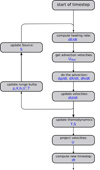 |
Fig. 1. Flow chart of the modified time advancement algorithm. The computed or updated quantities of each sub step are given in blue. |
During the RK loop we need to introduce two additional velocities in the scheme. U* is the updated velocity in each RK step, computed using the reconstructed velocity at cell interfaces UMAC, which is forced to fulfil the velocity constraint (Eq. (1)), while U* does not do this in general.
In order to demonstrate the capability of the new time integration scheme, we set up a stable atmosphere with several g-mode cavities. We use a constant gravity and a linearly declining density, modulated by a sine function (avoiding density inversions). After integrating the hydrostatic equilibrium (HSE), we end up with a stratification that has several peaks in the Brunt-Vaisala-Frequency (see black line in Fig. 2).
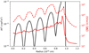 |
Fig. 2. Horizontally averaged profiles of a constructed stable atmosphere. The black solid line shows the initial N2 profile. Red lines give the velocity magnitude profile after 3 105 s for the predictor-corrector scheme (dashed) and the Runge-Kutta integrator (solid), respectively. |
A stable atmosphere should not develop significant velocities, yet Fig. 2 shows that the predictor-corrector method produces large velocities. After 3 105 s the profile exhibits a peaked velocity profile. The peaks coincide with the N2 cavities and they increase in amplitude as N2 increases. The reason for the peaks is the presence of numerical artefacts that act as high frequency gravity waves. Such artefacts will be trapped in the g-mode cavities and pile up over time until the waves break. Breaking gravity waves can develop a mean flow as has been shown in previous studies (e.g., Couston et al. 2018). The drop in velocity magnitude after the last peak in N2 is due to a velocity damping that is applied to reduce boundary effects.
In test simulations of convective boundary mixing, we found that this numerical phenomenon can create mean flows of a velocity magnitude similar to that of the convective motions. The RK integrator, on the other hand, smoothes the numerical artefacts such that we do not see this phenomenon any longer. The velocities get reduced by more than one order of magnitude (see red line in Fig. 2), and are now significantly smaller than the expected convective velocities.
Maestro is a purely Cartesian code with a one-dimensional background state. In order to compute spherical stars it is therefore necessary to adjust the scheme, such that the background state is evaluated consistently with the domain centred dataset. Nonaka et al. (2010) proposed the necessary algorithm to guarantee this in three-dimensional simulations. We extended their scheme to allow also for two-dimensional simulations of spherical datasets. The resulting domain is a planar slice through the star containing its centre.
2.2. Microphysics
In the Maestro simulations we use the Helmholtz equation of state (Timmes & Swesty 2000). Therefore our equation of state includes effects of radiation, ionization, degeneracy of electrons and Coulomb corrections.
The nuclear heating term is based on hydrogen burning equilibrium rates for the PP and the CNO cycle (Kippenhahn et al. 2012). We followed the evolution of three independent species (H, He, CNO) during the simulation, CNO species representing the total abundance of elements involved in the CNO cycle. Its atomic weight and charge is calculated according to the ratio of solar abundances of C, N, and O. The equilibrium rates reproduce the nuclear energy generation of the one-dimensional models within a factor of two.
In contrast to most other simulations of convective boundary mixing (e.g., Meakin & Arnett 2007; Cristini et al. 2017) we do not increase our energy production by an additional boosting factor in any of our simulations. This is possible because the timestep size of Maestro increases as the flow velocity decreases, and hence the number of convective turnover times that one can simulate does not depend on the absolute value of the flow velocity.
We also include energy transport by radiative diffusion using the analytic stellar opacities provided by Timmes (2000), which combine analytic expressions for hydrogen-free and hydrogen-containing compositions by Iben (1975) and Christy (1966), respectively. The opacities also contain contributions from Compton-scattering based on Weaver et al. (1978).
2.3. Initial models
We obtain our initial models with the one-dimensional stellar evolution code Garstec (Weiss & Schlattl 2008), and evolve them until the beginning of core hydrogen burning when less than 1% of hydrogen has been consumed. This leads to a very shallow jump in the hydrogen profile at the boundary of the convectively mixed core. Therefore, changes in the hydrogen profile can be seen quickly. Consequently, this quick reaction time of the conditions at the boundary also allows us to study the time evolution of the mixing.
For our calibration method (see Sect. 3.4) we need initial one-dimensional models computed with and without convective overshooting. Garstec implements overshooting as a diffusive process according to Freytag et al. (1996), where a diffusion constant D is computed based on the pressure scale height Hp and the distance to the convective boundary cz as
 (11)
(11)
with fov being the overshooting parameter and D0 the diffusion constant at the convective boundary. In Garstec D0 is evaluated inside the CZ at some distance to the boundary, since MLT predicts that the velocity as well as the diffusivity vanish right at the convective boundary.
Our models that include overshooting start from the same initial conditions as the non-overshooting ones and are self-consistently evolved until they reach a similar central hydrogen content as the models without overshooting. As a consequence of our self-consistent approach and the fact that we assume a radiative temperature stratification in the overshooting region, we find that the size of the convective core according to the Schwarzschild criterion in the one-dimensional models increases slightly as we increase the overshooting parameter. The size of the mixed core, on the other hand, increases at a much large rate.
Garstec provides us with thermally relaxed models on a Lagrangian grid. In order to map these into Maestro, we need to interpolate the model onto an Eulerian grid. The interpolation introduces slight deviations from HSE in the mapped models. Since Maestro expects its background state to be in perfect HSE, it is necessary to reintegrate the equation of HSE:
 (12)
(12)
During this reintegration, we also switch from the OPAL equation of state used in Garstec to the Helmholtz EOS in Maestro, which slightly modifies the thermal structure of the models, and thus no longer guarantees thermal equilibrium. MLT predicts the temperature gradient in the CZ of our models to correspond to a small overadiabaticity of the order of 10−8. Because overadiabacity acts as an energy reservoir for the convective flow in a hydrodynamic simulation, a small change in the temperature stratification can increase the internally stored energy significantly or remove the convective core entirely. To keep the simulations energetically as close as possible to the initial models, we take the MLT temperature gradient ∇mlt into account while recalculating HSE. For that purpose we substitute the temperature gradient ∇ by ∇mlt, so that
 (13)
(13)
where ∇ex is the superadiabaticity.
We achieve this requirement by simultaneously solving Eqs. (12) and (13), which also ensures that the location of the convective boundary does not change during the reintegration as has been shown by Edelmann et al. (2017). In Fig. 3 we demonstrate the effect of this integration method. Models that are reintegrated while keeping the temperature constant (red dotted line) lead to a temperature stratification that is stable in the very centre of the convective core and largely superadiabatic towards the convective boundary. Keeping the overadiabaticity constant instead (red solid line), we achieve a much more consistent temperature stratification. With this procedure we get a HSE with a relative accuracy of 10−5 and a temperature gradient that is only 5 10−5 larger than the adiabatic temperature gradient in the CZ. While this value is still three orders of magnitude larger than that predicted by MLT (red dashed line), it is sufficiently small for the purpose of our simulations. In Fig. 3 we also display the density profile before (dashed black line) and after reintegration (solid black line). The change in the density profile introduced by the reintegration is within the thickness of the plotted line, and hence can be neglected.
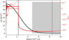 |
Fig. 3. Initial density (black) and superadiabaticity (red) of the model H3.5 (solid; see Table 1) and H3.5-T (dotted), respectively. Dashed lines give the stratification as predicted by Garstec. The vertical dashed and dotted lines indicate the boundary of the convective core and of the computational domain, respectively. In the shaded region we damp the velocities. |
3. An intermediate mass star
An intermediate mass star on the main-sequence has a mass between ≈1.2 M⊙ and ≈8 M⊙, a convective core, and a radiative envelope. Such stars are not massive enough to evolve all the way to core collapse and will end their life as a carbon-oxygen white dwarf. Here we discuss two-dimensional simulations of the convective core in a 3.5 M⊙ star with a solar like composition of X = 0.710, Y = 0.276, and CNO = 0.014. We chose this mass, because it has a convective core large enough to avoid problems with our overshooting description (see Sect. 2.3). Intermediate mass stars are also preferred targets for observers to study IGW. Using the observed frequencies of IGW, originating at the boundary of the convective core, it is possible to estimate the sizes of the mixed cores (Deheuvels et al. 2016; Moravveji et al. 2016).
Our simulations cover the complete convective core on a Cartesian grid as well as the star’s stable layer up to roughly 50% of the stellar radius. This corresponds to a total of six pressure scale heights and five density scale heights (see Fig. 3). Gilet (2012) showed that mapping and averaging errors in the corners of the Cartesian grid can lead to spurious velocities that quickly grow in amplitude. To reduce this influence we apply a velocity damping in the outer parts of the computational domain following Almgren et al. (2008). The shaded region in Fig. 3 shows to the damping region, whose inner boundary is located at a radius of 4.8 1010 cm.
Robinson et al. (2003) found that velocities and temperatures are strongly influenced by domain boundaries up to a distance of at least two pressure scale heights. Hence, our velocity damping starts only ≈2.5 pressure scale heights beyond the convective boundary, thereby reducing such boundary effects.
We performed ten simulations in total, exploring the effects of overshooting, time integration, initial model preparation, and resolution in time and space (see Table 1). Our longest running simulation spans more than 6 years of physical time and covers roughly 340 convective turnover timescales.
Overview of our two-dimensional simulations of a 3.5 M⊙ star.
3.1. Onset of convection and steady state properties
We initialize all of our simulations by imposing a small velocity perturbation in the inner part of the CZ as in Zingale et al. (2009). The perturbation quickly grows and causes a pronounced peak in the density-averaged convective velocity amplitude  after ≈105 s (see Fig. 4). Similar transients have been seen in other simulations (e.g., Meakin & Arnett 2007; Jones et al. 2017; Gilet et al. 2013). The transient is connected to a release of thermal energy in the CZ, which brings the slightly overadiabatic temperature gradient closer to the adiabatic one. Subsequently, the density-averaged convective velocities slowly dissipate away over a few convective turnover times until they reach a quasi steady state after around 107 s. Their values are then quite similar in simulations of different resolution (Fig. 4), indicating convergence. We also performed simulations with the original predictor-corrector scheme (denoted with PC in Col. 7 of Table 1) of Maestro and found that we reach a similar quasi steady state as with our 4th order Runge-Kutta time integrator (denoted with RK in Col. 7 of Table 1).
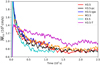 |
Fig. 4. Evolution of the density-averaged convective velocity magnitude |

The simulation H3.5-T uses an initial profile where the temperature of the one-dimensional model was preserved during reintegration of the HSE. This simulation produces during the whole simulation ≈30% larger convective velocities than the models initialized with a preserved ∇ex, which indicates that the initial thermal energy reservoir acts as an additional non negligible heating source in H3.5-T.
The velocity field in the CZ is dominated by two counter-rotating vortices (see left panels in Fig. 5), which is a well known effect due to vorticity conservation in two-dimensional simulations (e.g., Kercek et al. 1998; Meakin & Arnett 2007). As expected from the inverse energy cascade in two-dimensional simulations (Kraichnan 1967; Batchelor 1969), the vortices fill as much space as is available in the CZ.
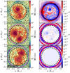 |
Fig. 5. Velocity magnitude (left panels) and deviations of the hydrogen mass fraction from its angulary averaged value X′(x, y) = X(x, y)−⟨X⟩(r) (right panels) of simulation H3.5, H3.5-ov1.7, and H3.5-ov3.0 (from top to bottom) after 2 107 s. The magenta dashed circles mark the initial size of the mixed core, while the black dashed circles show the size of the convective core according to the Schwarzschild criterion. The streamlines in the left panels indicate the flow direction. |
Figure 6 shows velocity magnitude profiles ⟨⟨|U|⟩⟩t, which are first angularly averaged (indicated by ⟨.⟩), and then averaged in time (⟨.⟩t). Angularly averages are performed using the yt python package (Turk et al. 2011), which sorts the Cartesian cells into radial bins based on the central point of each cell, and then computes a mass weighted average for each bin. The time average is performed over 50 output files between 5 106 s and 107 s, which corresponds to roughly ten convective turnover timescales. Overall, the shape of the velocity profile within the CZ follows the predictions by MLT (black dashed line in Fig. 6) in all simulations. However, the velocities are larger by more than one order of magnitude. Similar discrepancies were also found in other two-dimensional simulations (Meakin & Arnett 2007; Pratt et al. 2016). Meakin & Arnett (2007) and Pratt et al. (2020) confirmed that the higher velocities are an artefact of the reduced dimensionality of two-dimensional simulations.
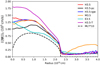 |
Fig. 6. Time-averaged velocity profiles for different two-dimensional simulations of a 3.5 M⊙ star. The averages extend from 5 106 s to 107 s. The dashed black line shows, scaled up by a factor of 10, the velocity profile predicted by MLT. |
Besides the shift in amplitude we also find that contrary to MLT predictions the velocity peaks in our simulations in the centre of the star. This demonstrates a shortcoming of MLT, which treats the centre of the star as a convective boundary and therefore predicts zero velocity at that point. Our simulations do not suffer from this shortcoming due the usage of a Cartesian grid, which allows flows across the centre of the star. MLT also predicts that the velocities should drop to zero at the boundary of the CZ. Instead, we find a noticeable velocity magnitude throughout the stable layer, which is approximately one order of magnitude smaller than in the CZ. The latter behaviour does not hold, however, for the medium resolution model M3.5, which suffers from the problem of unresolved gravity waves as discussed in Sect. 2.1. Nevertheless, in the CZ the velocity profile of model M3.5 agrees perfectly with that of model H3.5 indicating that the time-averaged flow in the CZ is numerically converged. The small discrepancies present between model H3.5 and the extremely highly resolved model E3.5 can be explained by the different transient behaviours of these simulations (see Fig. 4), because model E3.5 reaches the quasi steady state at an earlier time than model H3.5, which reduces the average velocities in model E3.5.
In simulation H3.5-igw we used the timestep criterion according to Eq. (10), which resolves the timescale of IGW up to a wavelength of a pressure scale height. For efficiency reasons we used the PC integrator in this case. According to linear theory IGW are exponentially damped inside of a CZ, which means that we do not expect any influence of unresolved IGW on the convective flow itself. Figures 4 and 6 show that models H3.5-igw and H3.5 indeed produce almost identical results in the CZ.
Simulation H3.5-igw also confirms the need for a higher order time integration. Figure 6 shows that model H3.5-pc, which uses the original PC time integration, has consistently smaller velocities than those found in model H3.5. However, the results of simulation H3.5-igw, which were obtained with the same timestep integrator but smaller timesteps than model H3.5, agree perfectly with those of model H3.5.
3.2. Convective boundary
Before we can discuss the mixing across convective boundaries in more detail we first need to define the position of the convective boundary. In a one-dimensional stellar evolution context the most commonly used definition is the Schwarzschild boundary, namely the point where the acceleration of mass elements by buoyancy is no longer positive. A proxy for the Schwarzschild criterion is a negative superadiabaticity ∇ex as defined in Eq. (13). We denote the corresponding radial position by Rstruc.
In hydrodynamic simulations, however, the position of a convective boundary can also be determined by the velocity field. Rogers (2015) and Brummell et al. (2002) account for this by defining the position of the convective boundary as the point where the kinetic energy Ekin drops to 1% or 5% of its peak value, respectively. We propose instead to use the standard deviation of a dynamical quantity as an indicator for the boundary, because time-averaged profiles smooth out all rare mixing events that might happen during the averaging period. Pratt et al. (2017) argue that such rare mixing events will set the final depth of the mixed region around CZ. Using the standard deviation of the velocity field (or kinetic energy field) does include a larger contribution from those rare events into the time average.
To this end we define the time-averaged standard deviation ⟨σ(Ekin)⟩t by combining the standard deviations σi(Ekin) of N output files as
![Mathematical equation: $$ \begin{aligned} \langle \sigma (E_{\mathrm{kin} })\rangle _t = \left[\frac{\sum _{i = 0}^{N} \sigma _i(E_{\mathrm{kin} }) \left[ \langle E_{\mathrm{kin} ,i}\rangle - \overline{\langle E_{\mathrm{kin} }\rangle } \right]^2}{N} \right]^{1/2}, \end{aligned} $$](/articles/aa/full_html/2021/02/aa39532-20/aa39532-20-eq16.gif) (14)
(14)
where  is the mean of ⟨Ekin, i⟩.
We define the boundary Rdyn (see Fig. 7) to be located at 5% of the maximum value of ⟨σ(Ekin)⟩t. In Fig. 7 we also show for comparison the profiles of ⟨⟨Ekin⟩⟩t and ⟨⟨Uϕ⟩⟩t. As expected Rdyn is located at a larger radius than a boundary that is defined at 5% of the maximum value of ⟨⟨Ekin⟩⟩t. Figure 7 shows that our definition of Rdyn provides a radial position of the boundary that is very close to the steepest gradient in the angular velocity component Uϕ, which was shown to be a good indicator for the convective boundary by Jones et al. (2017).
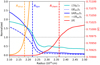 |
Fig. 7. Various radial profiles in the neigbourhood of the convective boundary. ⟨⟨Uϕ⟩⟩t, ⟨⟨Ekin⟩⟩t, and ⟨⟨∇ex⟩⟩t are the combined spatial (indicated by ⟨.⟩) and time (⟨.⟩t) averages of the angular velocity Uϕ, the kinetic energy Ekin, and the superadiabaticity ∇ex = ∇mlt − ∇ad, respectively. The time averages are taken from 1.82 108 s to 2.06 108 s using 100 output files from the H3.5 simulation. ⟨σ(Ekin)⟩t is the time-averaged standard deviation of the kinetic energy (see Eq. (14)). The angularly averaged hydrogen mass fraction profile ⟨X⟩ is taken at 2.06 108 s. The curves of ⟨⟨Uϕ⟩⟩t, ⟨⟨Ekin⟩⟩t, ⟨⟨∇ex⟩⟩t, and ⟨σ(Ekin)⟩t are normalized to the values corresponding to their respective boundary definitions (see text), which means that the black dotted line indicates the boundary values of each line. The dashed vertical lines mark the radial locations of our favoured boundaries. |
Another way how to determine the CZ boundary was used by Cristini et al. (2017) and Meakin & Arnett (2007), who followed the evolution of the size of a CZ by looking at the time evolution of the chemical composition which, in general, has an initial jump at the CZ boundary. The radial position where the composition corresponds to the mean between CZ and stable layer can then be defined as the boundary Rchem.
Figure 7 shows the respective time-averaged profiles obtained in our H3.5 simulation, and it also gives the corresponding locations of the various boundaries. We set the Schwarzschild boundary at ∇ex < −2 10−4 due to the uncertainty in this quantity in Maestro simulations (see Sect. 3.5). At the end of the simulation we find Rstruc < Rdyn < Rchem.
In order to understand how mixing across the boundary progresses we can now look at the time evolution of the different boundary definitions. Figure 8 shows that the boundaries Rdyn and Rstruc are constant during the whole simulation, except for the transient phase at the beginning. During the transient the location of Rstruc is shifted inwards by about 7 108 cm, indicating a thermal restructuring due to the release of thermal energy stored in the temperature gradient. The released thermal energy is converted into kinetic energy, which shifts Rdyn outwards beyond the initial location of Rstruc at 2.25 1010 cm. Once Rstruc retracts and the system approaches a quasi steady state Rdyn remains constant.
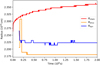 |
Fig. 8. Temporal evolution of the various convective boundary locations (see text) in the H3.5 simulation. |
The spatial ordering of the boundaries is in agreement with the simple picture of ballistic overshooting, which requires that mass elements penetrate into the layer beyond the Schwarzschild boundary. The additional motion is reflected by the fact that Rdyn > Rstruc during most of the time. In fact, the short period in the beginning of the simulation where the order is reversed is due to chemical mixing, which adjusts the shape of the temperature gradient to the more realistic Ledoux criterion. This effect temporarily increases ∇ just outside of the initial Schwarzschild boundary. As the chemical boundary moves further out the change of ∇ due to chemical gradients becomes negligible for the determination of Rstruc, and the expected order is re-established. We also see that the distance between Rdyn and Rstruc is only 6 108 cm, corresponding to 0.04 Hp.
Lattanzio et al. (2017) give a limit of mixing around CZ during thermal pulses of asymptotic giant branch stars. They argue that the maximum distance a plume can mix is set by its kinetic energy and the counteracting buoyancy force. For a general density ρ(r) and gravity g(r) stratification one can then calculate the penetration depth d = |r1−r0| as
 (15)
(15)
where ρp is the density of the plume and v0 its typical velocity. Assuming that a plume reaches the boundary with a velocity that corresponds to the maximum of the velocity profile in Fig. 6 (v0 = 1.4 105 cm s−1) and that its density corresponds to the density at the boundary (ρp = ρ(r0)) the maximum penetration length is d = 5 107 cm, which is considerably smaller than what our simulations show. If we additionally account for the expansion of the plume by requiring its density to be always a fraction of 10−4 larger (which is a typical value we find in our simulations) than the surrounding density such that ρp = ρ(r)(1 + 10−4), we find d = 5 108 cm in very good agreement with our measured distance between Rdyn and Rstruc.
However, we also see that the chemical boundary is evolving further into the stable layer throughout the simulation, indicating that model H3.5 experiences a constant mixing of hydrogen across its core boundary. Furthermore, Rchem becomes much larger than Rdyn, which shows that the ballistic overshooting cannot be the main mixing process, as it does not reach that far into the stable layer. In the following we therefore look at diffusive mixing processes that can contribute to the effects we see.
3.3. Diffusive mixing
As was shown by Rogers & McElwaine (2017), IGW can mix the stable layer of stars diffusively. Even though we do not fully resolve the highest frequency IGW in our simulations they still develop a rich IGW spectrum, best seen by looking at temperature fluctuations T′(r, ϕ) = T(r, ϕ)−⟨T⟩(r) around the angularly averaged temperature ⟨T⟩(r), where T(r, ϕ) is our Cartesian temperature field interpolated onto a polar grid.
In Fig. 9, which shows temperature fluctuations in model H3.5 at 8 107 s, one can recognize a clear distinction between the CZ with an almost homogeneous temperature distribution except for the centre of the vortices (bright spots) and the stable layer, which shows orders of magnitude larger temperature fluctuations. The regular flat pattern in the stable region indicates that the convective flow creating the IGW is dominated by large vortices (Rogers et al. 2013). Since this is an effect of the reduced dimensionality of our simulations, we do not expect this wave pattern to be a good representation of nature and therefore will not analyse it in detail.
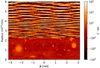 |
Fig. 9. Temperature fluctuations around the angularly average value in the H3.5 simulation at 8 107 s. |
Because the mixing caused by these waves plays a significant role in our analysis, we estimated the amount of diffusive mixing by IGW with tracer particles in a post processing step. Following Rogers & McElwaine (2017) we used tracer particles and tracked how the particles were advected by the flow. For that purpose, the velocities of the tracer particles are estimated via linear interpolation on the grid. The positions of the tracer particles are then evolved with a constant velocity up until the time of the next simulation output. To increase the accuracy of the analysis we increased the number of simulation outputs during the analysed timespan by a factor of 1000, that is one simulation output every 1000 seconds. We placed the tracer particles on regularly spaced spherical shells with radii between 2.0 1010 cm and 4.0 1010 cm to increase the resolution in the CZ boundary region (see top left panel of Fig. 10). The radial diffusion coefficient D at radius r is then the average of the squared radial displacement of the tracer particles initially placed at r divided by the elapsed time.
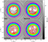 |
Fig. 10. Distribution of tracer particles for model H3.5 at several epochs. We show only 4000 of the 40 000 tracer particles used in the simulation, which are coloured according to their initial radial location given in the upper left panel. |
Figure 10 shows snapshot of the position of the tracer particles for model H3.5. Already early on the particles initially located inside the CZ get transported all the way to the centre and eventually get almost homogeneously distributed inside the CZ. This demonstrates the efficiency of convective mixing, corresponding to a large radial diffusion coefficient of D ≥ 1013 cm2 s−1 (see Fig. 11). This value is in perfect agreement with the value of diffusion coefficients estimated from MLT velocities. Even though we can compute D inside the CZ we want to note here that a diffusive treatment of convective mixing is not correct, because the extracted value of D depends on the chosen Δt (see Rogers & McElwaine 2017). In particular, one would expect that D ∝ 1/Δt once the tracer particles are randomly distributed inside the CZ, since the mean radial displacement cannot increase further at that point unless particles are mixed from the CZ into the stable layer. We also want to emphasize that the diffusion coefficients estimated here do not apply to other stars with a different density or temperature stratification.
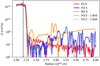 |
Fig. 11. Radial diffusion coefficients estimated from the advection of 40 000 tracer particles followed for 1.5 106 s for models of different grid size. The dashed and dotted lines labelled ‘H3.5 – 1.6e5’ and ‘H3.5 – 1.0e6’ represent the same quantity but evaluated with 160 000 and 106 tracer particles in model H3.5, respectively. The dashed vertical line indicates Rdyn of model H3.5. |
Outside of the CZ the tracer particles move considerably less. At later times there is some mixing between the particles, but mainly in the lateral direction as can be seen from the colour coding in Fig. 10. The mean of the squared radial displacement of tracer particles at three initial radial positions in the stable layer is given in Fig. 12. A diffusive process will on average lead to a linear growth of the squared radial displacement. Our measurements show that a clear linear trend is maintained until 1.5 106 s. After that point integration errors become noticeable and the curve slightly deviates from its linear trend. In the following we therefore only consider the first 1.5 106 s of the tracer particle movements to estimate diffusion coefficients. We performed this analysis with 40 000, 160 000, and 106 tracer particles, where the latter corresponds to about four tracer particles per grid cell in the analysed radial range. In Fig. 12 the different symbols – corresponding to the number of tracer particles used – show that the number of tracer particles has little influence on the measured radial displacement, indicating convergence of the analysis method. In the following we therefore use 40 000 tracer particles.
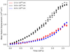 |
Fig. 12. Time evolution of the mean squared radial displacement of tracer particles in model H3.5. The particles which where used for the analysis were taken at r = 2.5 106 cm, 3.0 106 cm, and 4.0 106 cm. Stars, diamonds, and crosses correspond to analysis runs with a total of 40 000, 160 000, and 106 tracer particles, respectively. |
Measuring D for all radial values, we find that D is orders of magnitude smaller in the stable layer than in the CZ (see Fig. 11). In the transition region between the CZ and the stable layer D drops sharply at R ≈ 2.25 1010 cm, corresponding to our dynamical convective boundary Rdyn. Therefore, we interpret the drop in D as a very rapid decline of dynamical convective mixing in that region. Overall we find good agreement with the results of Rogers & McElwaine (2017), who analysed a 3.0 M⊙ star at the zero-age-main-sequence (ZAMS). This setup is very similar to the one in this work and therefore directly comparable. Rogers & McElwaine (2017) also find D ≈ 1013 cm2 s−1 in the CZ, and then a sharp drop to D ≈ 108 − 109 cm2 s−1 in the stable layer, which is approximately 1–2 orders of magnitude smaller than what we find. Here it should be noted that D = 109 cm2 s−1 corresponds to an average diffusion distance of roughly one third of a computational cell of model H3.5 during the analysed period of 1.5 106 s. Hence, we estimated the systematic error in the value of D by repeating the analysis with our medium resolution model M3.5 and the extremely high resolution model E3.5 (see Fig. 11).
We find that all three simulations give identical values of D in the CZ, showing that the convective motions are converged. The same is true for the location and steepness of the sharp drop of D at the dynamical boundary (see Fig. 11). However, we find rather large differences of up to four orders of magnitude in the stable layer. As mentioned before, we attribute this to the limited spatial resolution of our simulations. We would expect to find smaller and smaller values of D if we increase the resolution further as suggested by the small values of D found in model E3.5.
The hypothesis that our values of D are overestimated is also supported by timescale arguments. Using the low values of D = 107 cm2 s−1 found in model E3.5, we find that the mixed core will grow by ≈0.4 Hp during its local thermal timescale of 160 kyr. Considering the main-sequence lifetime of a 3.5 M⊙ star of the order of 100 Myr one consequently finds that the whole star will be fully mixed at the end of the main-sequence. Moreover asteroseismic observations of KIC 7760680 by Moravveji et al. (2016) found that stellar models can only fit the observed frequencies when an additional diffusive mixing is added throughout the stable layer. They determined a value of D ≈ 10 cm2 s−1. A simulation that could resolve such small diffusion coefficients is computationally infeasible.
Overall we conclude that there is some diffusive mixing due to IGW in our simulations, but it is very likely that the amount we find is largely overestimating the mixing in actual stars. The most likely reason for this is the limited resolution of our simulations, which does not allow us to properly handle significantly smaller values of D. The increased convective velocities in our two-dimensional simulations (see Sect. 3.1) probably also caused values of D that are overestimated.
3.4. Overshooting calibration
The large difference between the short dynamical timescale of convection and the long nuclear timescale of stellar evolution prohibits the simulation of multi-D stellar evolution models with current computers. Therefore, one-dimensional stellar evolution models still rely on parametrized models of convection. A crucial parameter in this approach is the overshooting parameter which sets the size of the mixed region around a CZ. In this section we show how one can use multi-D simulations to estimate the one-dimensional overshooting parameter.
To this end we analysed the evolution of the hydrogen mass fraction X in the CZ in our multi-D simulations. Initially hydrogen is distributed homogeneously in the CZ, and the adjacent stable layer has a larger hydrogen mass fraction than the CZ. One way to quantify the mixing efficiency across the convective boundary is to examine the increase of the total hydogen mass inside the CZ MX with time. For this purpose we set the location of the convective boundary at the Schwarzschild boundary of the initial model, which is not necessarily the same as Rstruc because the temperature stratification changes slightly during the initial transient. Furthermore, we denote MX at t = 0 by MX0.
Figure 13 shows the mixing during the initial transient and the beginning of the quasi steady state for the same models as in Figs. 4 and 6. MX increases by (2.0 ± 0.5) 10−5 M⊙ during the first 107 s in all simulations, except for model H3.5-T for which the amount of mixing is about twice as high as that of, for example model H3.5. This enhanced mixing is due to the fact that the velocity is on average larger in the steady state of model H3.5-T, and that the model also experienced a more extended transient phase (see Fig. 4) with even larger velocities. The duration of the transient is also the reason for the small differences in mixing between the medium and extremely high resolution models M3.5 and E3.5. However, once the simulations reach the quasi steady state the mixing evolves at very similar mixing rates, which is confirmed by looking at the time derivative ṀX shown in the bottom panel of Fig. 13.
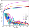 |
Fig. 13. Change in the hydrogen mass for the initial convective core of our 3.5 M⊙ simulations. The top and bottom panels show the hydrogen mass relative to its initial value and the corresponding rate of change, respectively. |
It is also worth noting here that the mixing rates in models H3.5 and H3.5-igw agree almost perfectly. This confirms the hypothesis we made in Sect. 2.1 that the unresolved high frequency IGW in model H3.5 do not contribute to the mixing significantly.
Figure 14 shows the long-term evolution of mixing in model H3.5. Averaging the mixing rate for t > 107 s we find ṀX = 4.010−6 M⊙ yr−1. Over its main-sequence lifetime this star’s overshooting region would therefore consume the unrealistic amount of > 400 M⊙. However, as the bottom panel of Fig. 14 shows, ṀX is slightly declining with time, and the outward motion of Rchem is also slowing down with time (see Fig. 8). Hence, over the evolutionary timescale of stellar models we would expect that this trend eventually leads to an end of mixing, at which point the final location of Rchem would be reached. However, as the thermal evolutionary timescale of a 3.5 M⊙ star on the ZAMS is of the order of 105 yr and as we are only able to simulate ≈6 yr of steady convection, extrapolating our results over five orders of magnitude is prone to large uncertainties. Therefore, we propose a different method to estimate the maximum extent of the mixed region by comparing simulations performed with initial models with the same mass and evolutionary state but computed with different values of the overshooting parameter fov. Increasing fov will increase the mass of the initially homogeneously mixed region Mmixed, i, and due to our self-consistent treatment of the evolution of the overshooting models (see Sect. 2.3) we also get slightly different masses MCZ, i for the convective core as defined by the Schwarzschild criterion (see Table 1).
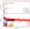 |
Fig. 14. Same as Fig. 13, but for simulations performed with different fov values. The vertical dashed line indicates t = 2 107 s. |
In order to explain the idea behind this method, we first need to look at the process of mixing in more detail. As we have already discussed in Sect. 3.1, we find that the convective flow is dominated by two large vortices. These vortices produce shear mixing at the convective boundary, which can be best seen by looking at the horizontal perturbation of the hydrogen mass fraction X′(x, y) = X(x, y)−⟨X⟩(r). We provide snapshots of this quantity in the right panels of Fig. 5. The prominent large scale inflow of hydrogen from the left into the CZ visible in the top right panel of Fig. 5 suggests that mixing is largely localized, and that the rather constant mixing rate one sees in Fig. 14 is in reality a combination of single localized mixing events. We argue that each of these mixing events will affect a maximum distance from the convective boundary from where it can collect material with larger X. Pratt et al. (2017) make a similar argument based on plumes penetrating the boundary of a convective envelope, and they show that the plumes with the largest mixing depth will eventually set the maximum extent of the overshooting region.
Our calibration of fov works on the basis of this Extreme Value approach, and is illustrated in Fig. 15. In a simulation performed with an initial model without any overshooting Rchem (vertical lines in Fig. 15) and Rstruc will initially overlap. In other words, each single mixing event across the convective boundary (represented by plumes in Fig. 15) will reach regions with a larger X, and will transport some of the excess hydrogen into the CZ. As Rchem moves further out into the stable layer due to mixing, less and less mixing events will be able to reach hydrogen rich matter. This effect reduces the mixing as indicated by the sequence of arrows at the top of Fig. 15.
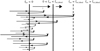 |
Fig. 15. Illustration of our overshooting calibration method (see text). |
By setting up simulations performed with initial models computed with fov > 0 we try to find the numerical value fov, ideal that results in a mixed core that exactly reproduces the extent of the mixed region in a long-term simulation. For values slightly smaller than fov, ideal we would then expect to see a very small increase of MX over time, while we would see none for values larger than fov, ideal. The initial state of simulations performed with fov > 0 might not fully reflect the smeared out composition profile of a mixed model performed with fov = 0 for a long time. However, we would expect that the composition profile of such a long time mixed model steepens once the maximum extent of the mixed region has been reached. We expect that the discrepancy to a one-dimensional model with fov > 0 eventually decreases.
We compared the average mixing rate of three simulations setting fov equal to 0.01, 0.02, and 0.03, respectively. The respective simulation names are appended by ‘-ov’ followed by the value of fov times 100 (see Table 1). In addition, we performed a fourth simulation with fov = 0.017 (model H3.5-ov1.7). This value is based on a calibration of fov on observations of open clusters performed by Magic et al. (2010) with the Garstec code.
After 2 107 s all simulations have reached a quasi steady state and the velocity fields look qualitatively the same regardless of fov (see left panels of Fig. 5). Comparing the right panels of Fig. 5 from top to bottom, it is evident that increasing fov decreases the perturbation amplitude of the hydrogen mass fraction, which implies a less efficient mixing in models simulated with a large overshooting parameter.
We find that model H3.5 mixes 10−5 M⊙ of hydrogen into the core during the whole simulation. Increasing fov to 0.01 decreases the mixing rate by a factor of ≈2, which would still corresponds to a fully mixed star at the end of the main-sequence. However, increasing fov further leads to a massive drop in the mixing rate by more than one order of magnitude. The Kelvin-Helmholtz timescale of a 3.5 M⊙ star is ≈600 kyr, which means that models H3.5-ov1.7 and H3.5-ov2.0 will mix much less than 0.1 M⊙ of hydrogen into the core over a thermal timescale. This should allow the star to thermally adjust its structure to the new core size, especially when we consider that the local thermal timescale of the core is only about 150 kyr. Model H3.5-ov3.0 even does not mix any hydrogen at all during the simulation time, showing that fov = 0.03 is clearly too large.
We also find that increasing fov changes the characteristic of the time evolution of ṀX. While ṀX is more or less constant in models H3.5 and H3.5-ov1.0, it is dominated in models H3.5-ov1.7 and H3.5-ov2.0 by single peaks followed by a rather quiescent phase (see bottom panel in Fig. 14). One could interpret this behaviour as a mixing that is dominated by rare single mixing events, which means that only the farthest reaching mixing events contribute to the enrichment of hydrogen. However, the situation is more complex than that. After a careful analysis of the velocity field of model H3.5-ov2.0 between 4.9 and 5.7 107 s we could not find any mixing event that would bridge the distance of 0.1 Hp between Rdyn and Rchem. We see at most dynamic mixing to 0.05 Hp beyond Rdyn. The missing gap can be bridged by a diffusive mixing process with D = 1011 cm2 s−1 which slowly restores the composition profile before the next mixing event reaches the diffusion front. This value of D is larger than our estimate derived from model H3.5-ov2.0 (see Fig. 16). However, we also have to consider that such mixing events are highly localized in angle, which means that only a small angular section of the diffusion front is mixed into the core. Furthermore, angular diffusion is much larger than the radial one. Hence, it can easily smooth out the composition profile between mixing events in angular direction. Therefore, we argue that the episodic mixing behaviour seen in our simulations can be explained as an interplay between diffusive mixing and rare convective mixing events. Noh & Fernando (1993) performed a series of laboratory experiments with turbulence created by an oscillating grid. They found that the mixing across a convective boundary in water shows a similar episodic mixing behaviour as described above once the molecular diffusion in the experiments becomes dominant, thereby supporting our interpretation.
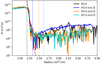 |
Fig. 16. Radial diffusion coefficients estimated from 40 000 tracer particles over 2.5 106 s for the models with different initial values of fov. The lines have been shifted such that the radial position of the structural boundary matches for all the simulations. The dotted vertical lines indicate the position of Rchem in each run. The red dashed line shows D according to Eq. (11) with fov = 0.01 |
We argued in Sect. 3.3 that diffusive mixing is most likely overestimated by several orders of magnitude in our models. Identifying the episodic mixing as a process dominated by diffusion then allows us to argue that models H3.5-ov1.7 and H3.5-ov2.0 would not show any mixing in a fully realistic setup. For our overshooting calibration method this assumption corresponds to 0.01 < fov, ideal < 0.017. We can compare this estimate to the asteroseismic constraints by Moravveji et al. (2016), who determined a value of fov = 0.024 for the 3.25 M⊙ star KIC 7760680. This value of fov is larger than the one we predict, but one should note that the absolute values of fov obtained with different codes should not be compared directly (see the discussion in Angelou et al. 2020). A more relevant evaluation of the result is to compare the mass of the overshooting region Mov in both cases. For model H3.5-ov1.7 we find Mov = 0.22 M⊙, which is in perfect agreement with the Mov = 0.2239 M⊙ found by Moravveji et al. (2016) in their grid B. Their favoured stellar model grid A, however, gives a larger value of Mov = 0.2642 M⊙.
We note here that while we calibrate fov according to Eq. (11) it is not clear whether Eq. (11) is indeed the best representation of the mixing processes around a convective core. To clarify this concern we repeated the exercise of calculating the radial diffusion coefficients for our calibration simulations by comparing the mixing beyond Rstruc in different runs. In Fig. 16, which shows the outcome of this exercise, we have radially shifted the Schwarzschild boundaries of the models such that they agree with each other. We find that all models give remarkably similar values of D in the CZ and around the drop due to the dynamical boundary Rdyn. In Sect. 3.3 we have also seen that the latter part of the profile of D is independent of grid size. The overshooting model defined by Freytag et al. (1996) (see Eq. (11)) is supposed to represent the run of D. Indeed we can fit the drop at Rdyn perfectly with this overshooting description and a value of fov = 0.01 (see red dashed line in Fig. 16), which is smaller than our estimated value. However, in contrast to this work Freytag et al. (1996) estimated the overshooting in convective envelopes. In other words, the convective plumes in Freytag et al. (1996) penetrate into regions with higher density. This has a huge impact on the behaviour of IGW, which are damped in Freytag et al. (1996) with increasing distance to the convective boundary, and are amplified in this work. The driving factor for the amplitude changes in both cases is that amplitudes of IGW scale as ρ−1/2. We can therefore assume that diffusive mixing by IGW is negligible in the simulations of Freytag et al. (1996), and that their overshooting description mainly captures the mixing caused by turbulent motions at the convective boundary.
Several groups have extended Eq. (11) to also account for diffusive mixing in radiative layers by means of hydrodynamical simulations and observations. Herwig et al. (2007) fitted the mixing in simulations of helium shell flashes on the asymptotic giant branch to two connected exponential functions with different slopes. From their simulations they determined fov to be 0.01 and 0.14 for the first and second exponential, respectively, which means that the sharp drop of D right at the convective boundary matches perfectly with our results. However, the second exponential, which Battino et al. (2016) interpret as additional diffusive mixing by IGW, is not present in our models. Fitting the asteroseismic observations of KIC 7760680 Moravveji et al. (2016) required that in addition to Eq. (11) a small constant diffusive mixing is present throughout the stable layer. Similarly Rogers & McElwaine (2017) also predict a diffusive mixing that is active in the whole radiative region, but their simulations indicate that the diffusivity actually increases with increasing distance to the CZ due to the amplification of IGW.
Our results do seem to support that there is a constant diffusion in the stable layer as proposed by Moravveji et al. (2016). However, due to the damping of velocities in the outer regions of our simulations we can only estimate D in a region relatively close to the convective boundary. At the maximum radius considered for the tracer particle analysis (= 4 106 cm) the density has dropped by a factor of two in respect to the convective boundary. Using the amplitude scaling of linear IGW, this corresponds to an increase of amplitude by ≈40%. A change that is hardly noticeable in our analysis where measured values of D regularly vary by two orders of magnitude and more in the stable layer (see Fig. 16). A further increase of D at larger distances to the convective boundary due to the amplification of IGW like in Rogers & McElwaine (2017) can therefore not be excluded.
However, in our overshooting calibration method we combine the effects of turbulent mixing and diffusive mixing by IGW into a single effective fov. We argue that due to the long evolutionary timescale on the main-sequence we do not expect that the mass of the overshooting region does depend on whether we use dedicated models for diffusive mixing and turbulent mixing or a single step overshooting description with an effective fov that covers both mixing regimes. Asteroseismic properties, on the other hand, are more sensitive to such changes (Pedersen et al. 2018; Michielsen et al. 2019).
3.5. Temperature gradients
Another uncertainty of one-dimensional stellar evolution is the shape of the temperature stratification in the overshooting region. On the one hand, the classical step overshooting method predicts a fully adiabatic stratification. The diffusive overshooting according to Eq. (11), on the other hand, relies on radiative energy transport. We have seen in Sect. 3.2 that Rdyn > Rstruc which implies that there will be some convective motion, and therefore also convective energy transport beyond the Schwarzschild boundary. Zahn (1991) calls this layer where convective energy transport is still relevant the penetration region. Such a penetration layer has been found in hydrodynamic simulations of red giants (Viallet et al. 2013) and the solar envelope (Korre et al. 2019) as well as in one-dimensional stellar evolutionary calculations where convection was modelled by one-dimensional averages of the hydrodynamic equations instead of MLT (Li 2017).
In order to see whether we also see penetration in our core convection simulation we first have to discuss one peculiarity of Maestro simulations. Due to the fractional step approach in the time evolution algorithm of Maestro, the EOS functions T(ρ, P) involving the pressure and T(ρ, h) involving the enthalpy give temperatures which differ relatively by about 10−4.
We used the enthalpy version both for the nuclear energy production and the radiative energy transport. Given the T(ρ, h) temperature stratification one has still some freedom in calculating the temperature gradient  . One can compute the derivative either with respect to the total pressure Ptot = P0 + π or with respect to the thermodynamically consistent pressure PEOS = P(ρ, T(ρ, h)). Since the effects of pressure perturbations π are only considered in the momentum equation (Eq. (5)) one can also decide to compute ∇ based on P0. Figure 17 illustrates the effect of these different choices for ∇ on the superadiabaticity ∇ex = ∇ − ∇ad in the CZ, where ∇ad is the adiabatic gradient provided by the EOS. While ∇ex computed with PEOS shows a mostly stably stratified CZ, using P0 or P0 + π increases ∇ex by ≈10−4 in the outer region of the CZ, which then classifies this region as unstable. On the one hand, the flow field of our simulations clearly does not correspond to a stable stratification throughout the CZ making the use of PEOS questionable. On the other hand, PEOS is the thermodynamically consistent way of computing ∇ex. We account for this dilemma by using a rather loose criterion for stability in our analysis, where regions with |∇ex|< 10−4 are considered marginally stable. In the stable layer, where ∇ = ∇rad ≪ ∇ad, this modified criterion has very little influence. In the further analysis, we use ∇ex as computed with P0 for simplicity, which has no effect on the results.
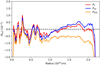 |
Fig. 17. Comparison of the different ways to compute the superadiabaticity ∇ex in Maestro simulations (see text for more details). Shown are angularly averaged profiles from model H3.5 at 108 s. |
The presence of a penetration layer can be detected by analysing the temporal evolution of the superadiabaticity ∇ex. In Fig. 18 we compare ∇ex after 4 107 s with the initial temperature stratification. In model H3.5 the Schwarzschild boundary moves inwards during the evolution, but at the same time ∇ex increases just outside of the initial CZ. This causes a bump in the superadiabaticity outside of the CZ, and brings the value of ∇ex very close to that of the adiabatic gradient, which interferes with our loose stability criterion, and therefore with the determination of Rstruc. When mixing progresses, the bump moves outwards where ∇ex decreases due to the increasing influence of ∇rad. The wave like feature exhibited by ∇ex (recognizable in Fig. 18) is due to the simultaneous mixing of both composition and thermal energy in simulation H3.5, which increases ∇ex due to the stabilizing effect of the molecular gradient  . Therefore, this feature resembles the curve derived from the Ledoux criterion
  , where
  , and
, and  .
.
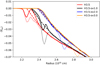 |
Fig. 18. Angularly averaged profiles of the superadiabaticity in models of a 3.5 M⊙ star with different amounts of overshooting. Dashed and solid lines show profiles according to the Schwarzschild criterion at t = 0 and after 4 107 s, respectively. The dotted lines give the initial profiles according to the Ledoux criterion. |
The same phenomenon can also be seen in model H3.5-ov1.0 but less prominent due to the larger initial distance between Rstruc and Rchem. At even larger distances between these radii, the wave like feature disappears completely as seen in models H3.5-ov2.0 and H3.5-ov3.0 (Fig. 18). In these simulations we instead see that the Schwarzschild boundary moves outwards at later times. Adjustments to the temperature stratification on timescales orders of magnitude shorter than the thermal timescale can be explained when we consider the effect of penetration as a balance between the competing processes of convective and radiative energy transport (van Ballegooijen 1982). Convection tries to establish an adiabatic temperature gradient, and will do so on a convective timescale. The counteracting radiative energy transport operates on much longer timescales so that our simulations establish a temporary penetration layer. Since we cannot simulate long enough to establish an equilibrium between those two processes, it is not possible to give an estimate of the actual size of the penetration layer. However, it is very likely that the final temperature stratification does not correspond to the one from the one-dimensional model, and instead will show some effects of penetration in the overshooting region.
4. Mass dependence
There is currently an ongoing discussion whether the overshooting parameter is depending on stellar mass or not. The discussion is mainly focusing on main-sequence stars, where core size correlates with mass in the mass range ≈1.2 M⊙ to ≈2.0 M⊙. Claret & Torres (2016) proposed a linear growth of the overshooting parameter with mass after calibrating stellar models to fit observations of eclipsing binaries. Similarly Pietrinferni et al. (2004) used a linear and VandenBerg et al. (2006) a tanh-like scaling of the overshooting parameters in their stellar evolution databases, which improves the fit of isochrones to open clusters with turn-off masses in the range of 1.25–1.8 M⊙. Other groups challenge these results based on asteroseismic observations (Deheuvels et al. 2016) or due to the lack of statistical significance (e.g., Constantino & Baraffe 2018; Stancliffe et al. 2015). With our calibration method we can contribute to this discussion with multi-D numerical simulations. Therefore, we computed three more sets of simulations with stellar masses of 1.3, 1.5, and 2.0M⊙ (see Table 2). As in the 3.5 M⊙ case we used ZAMS models with a solar metallicity.
Overview of our two-dimensional simulations of main-sequence stars of different masses.
4.1. 2.0 M⊙
In our three 2.0 M⊙ models we used slightly smaller values of fov than in the 3.5 M⊙ model, because model H2.0-ov1.0 with fov = 0.01 already showed the episodic mixing behaviour seen in models H3.5-ov1.7 and H3.5-ov2.0 (see Fig. 19). Following the same argumentation as before swe find that the diffusive mixing, which is overestimated in our simulations, implies that fov < 0.01. In order to establish a lower bound to this estimate, we then also computed model H2.0-ov0.5 with fov = 0.005 that showed a similar continuous mixing as model H2.0 with fov = 0, but at a slightly smaller mixing rate. Our estimate for this set of 2.0 M⊙ models is therefore 0.005 < fov < 0.01.
We can also compare this result with models of the eclipsing binary TZ For, where Higl et al. (2018) found that this relatively close system could not have undergone a mass transfer in its previous evolution, and that the mass of the helium core of the 2.05 M⊙ primary must have been at least 0.335 M⊙ (see their Table 2). This fits perfectly to our overshooting estimate where models H2.0-ov0.5 and H2.0-ov1.0 predict He-core masses of 0.32 and 0.37M⊙, respectively, assuming that the fully mixed core of the initial model corresponds to the He-core mass at the end of the main-sequence.
4.2. 1.5 M⊙
The pressure scale height at the boundary of the convective core of a 1.5 M⊙ star is 60% larger than the radial extent of the CZ itself. Using Eq. (11) with a moderate value of fov = 0.02, increases the mass of its mixed core by a factor of three compared to that of a no overshooting case. Therefore, we considered in our simulations smaller values of fov, which provide more reasonable core masses for a 1.5 M⊙ star.
Figure 20 shows that for this stellar mass the episodic mixing appears first in model H1.5-ov1.0 with fov = 0.01, hence providing the upper limit for our calibration. Model H1.5-0v0.5 with fov = 0.005 shows a continuous mixing behaviour resulting in an estimate of 0.005 < fov < 0.01. While this is exactly the same range of values as in the 2.0 M⊙ star, we should note that for the 1.5 M⊙ star fov = 0.005 gives a mixing rate that is only one order of magnitude larger than in the fov = 0.01 run, indicating that the ideal value of fov is much closer to 0.005 than to 0.01 considering that the same comparison in the 2.0 M⊙ star results in a difference of three orders of magnitude in ṀX. Asteroseismic observations by Yang (2016), on the other hand, suggest that the core of the ≈1.4 M⊙Kepler star KIC 9812850 has a radius of 0.140 ± 0.028 R⊙, which is in good agreement with the initial model of H1.5-ov1.0.
This 1.5 M⊙ models also allowed us to estimate a diffusion coefficient without the need of tracer particles. Models H1.5-ov1.0 and H1.5-ov2.0 both show an episodic mixing behaviour, but the onset in model H1.5-ov2.0 is delayed by ≈3 107 s. Considering that the distance between Rstruc and Rchem in model H1.5-ov2.0 is 1.1 109 cm larger than in model H1.5-ov1.0 one can estimate that D ≈ 4 1010 cm2 s−1, which is similar to the value found for the 3.5 M⊙ star even though the convective velocities in those models are twice as large as in the 1.5 M⊙ models. This again is suggesting that diffusive mixing is numerically overestimated in our simulations.
4.3. 1.3 M⊙
Since the pressure scale height diverges towards the centre of a star, a 1.3 M⊙ star has an even larger reaction to an unrestricted overshooting according to Eq. (11) than the 1.5 M⊙ models. In a 1.3 M⊙ star the mass of the mixed core increases by a factor of three even for a tiny overshooting parameter of fov = 0.005. Therefore, we did not compute any model with fov > 0.005 for this stellar mass.
As expected model H1.3-ov0.5 does show an episodic mixing behaviour (see Fig. 21). However, it also starts to develop a more continuous mixing at later times. In fact, we see that all models experience a sudden change in ṀX after ≈8 107 s, the reason being unclear. However, by examining the time evolution of the angularly averaged velocity of model H1.3 (Fig. 22) it becomes clear that the effect must originate in the stable layer. After 8 107 s the velocity pattern in the stable layer changes quickly from a wave like pattern to a homogeneous flow. This change starts deep in the stable layer and then propagates inwards. Once it reaches the convective boundary (marked by the white dashed line) the convective velocities become heavily suppressed. We see the opposite effect in models H1.3-ov0.25 and H1.3-ov0.5 where larger velocities lead to larger mixing rates, and in the case of model H1.3-ov0.5 to a switch from episodic mixing to continuous mixing.
It should be noted that the origin of the strange velocity pattern is located at around the same radial position as the N2 cavity of the stratification, suggesting that this effect is related to the resolution of IGW. This would also explain why there is an opposite effect in models H1.3-ov0.25 and H1.3-ov0.5 by a reflection of IGW at the N2 bump due to the composition interface. Furthermore, the wave pattern in model H1.3 also suggests that IGW seem to propagate inwards in this model as indicated by the black dashed line in Fig. 22.
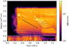 |
Fig. 22. Colour plot of the evolution of angularly averaged velocity magnitude profiles in model H1.3 during a timespan of 1.3 108 s. The radial position of the initial Schwarzschild boundary and the propagation direction of IGWs are marked by white and black dashed lines, respectively. |
It seems that simulations of a 1.3 M⊙ star are beyond the proper working limit of the RK time integrator, since numerically generated IGW dominate the evolution. It is, however, very unlikely that the numerical effects lead to less mixing than in a properly resolved simulation. Hence, we argue that an upper limit fov < 0.005 still holds, but we are not comfortable to give a lower limit on fov for this mass.
4.4. Overshooting parameter recommendation for one-dimensional models
Comparing our estimates for fov we see a clear trend towards smaller values for less massive stars. In order to ease comparison with stellar evolution models as well as with observations we provide also core masses in addition to the value of fov (see Col. 6 in Tables 1 and 2). In Fig. 23 we compare our hydrodynamic estimates with Garstec stellar evolution models computed with and without overshooting. Unsurprisingly all our hydrodynamic estimates predict core masses that are larger than those of models without overshooting. In our most massive 3.5 M⊙ star we find good agreement between our estimate and the commonly used value fov = 0.02. We note here that the data points of the one-dimensional models corresponding to fov = 0.02 were computed using Eq. (11) without any modification. Hence, the difference between our hydrodynamic values and those of the one-dimensional models increases as the pressure scale height at the convective core boundary increases due to the decreasing core size of less massive stars.
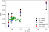 |
Fig. 23. Convectively mixed core mass for models with (black dots) and without overshooting (black stars) on the ZAMS. Blue and green ellipses show the same quantity, but using a geometrical cutoff for the overshooting and observational constraints by Mombarg et al. (2019), respectively. The red triangles denote the derived upper limits from our simulations. The black cross indicates the size of the mixed core of a 2.0 M⊙ star close to the end of its main-sequence evolution when the model is computed without overshooting. |
In models with small CZ Garstec usually applies a geometrical cutoff to prevent unrealistically large overshooting regions. The cutoff was introduced in Magic et al. (2010) and is based on a comparison of the pressure scale height at the convective boundary to the thickness of the CZ rcz itself. One introduces a reduced pressure scale height according to
 (16)
(16)
and applies the cutoff by replacing Hp in Eq. (11) with  . This approach was motivated in order to reproduce the morphology of the open cluster colour-magnitude diagram around the main-sequence turn-off of M67. The resulting core masses for fov = 0.02 are given in Fig. 23 as blue ellipses. We find that this cutoff is, in general, much more restrictive than our hydrodynamic estimates, which is also confirmed by Higl et al. (2018) who found that it is too restrictive to model the eclipsing binary TZ For.
We also compare our results with recent observations of γ Dor stars by Mombarg et al. (2019). These stars have typical masses of 1.5 M⊙ and oscillate due to the flux blocking mechanism, which excites gravity modes that allows one to probe the core region. The extracted core masses of 37 stars are shown in green in Fig. 23. We find a good agreement with our hydrodynamic estimates for stars around 1.5 M⊙, and also confirm once more that an overshooting cutoff according to Eq. (16) is too restrictive. A few of the observational estimates, however, contradict our results and show core masses that are even smaller than those in models without overshooting. This is due to a correlation between the central hydrogen content and the stellar mass in the analysis of Mombarg et al. (2019, see their Fig. 7). Larger stellar masses correspond to a smaller central hydrogen content, which means that stars with 2 M⊙ are already close to the end of their main-sequence evolution, when they have significantly smaller convective cores than on the ZAMS as indicated by the black cross in Fig. 23, which shows the size of the convective core at a central hydrogen content of 5%.
Overall we conclude that there is a general need for a mass-dependent overshooting description. However, we neither have enough datapoints to confirm the linear trend proposed by Claret & Torres (2016) nor do we have any other functional form of fov(M*). We also stress that this result only holds for convective core overshooting on the main-sequence and does not apply to convective envelopes or any other convective layer, as for example the intershell CZ in thermally pulsing AGB stars (Wagstaff et al. 2020).
4.5. Entrainment
Entrainment predicts that mixing across convective boundaries can be described as a constant growth, where the growth factor E is defined as (Turner 1986)
 (17)
(17)
where A and n are free parameters. The bulk Richardson number Rib is a measure of the stiffness of the boundary of a CZ, whereby convection is characterized by a typical lengthscale L and the rms velocity Urms of the flow. Rib can then be written as
 (18)
(18)
where Δb describes the buoyancy jump across a boundary of width di
 (19)
(19)
Meakin & Arnett (2007) found that an entrainment law according to Eq. (17) describes the mixing in an oxygen burning shell as well as that in a 25 M⊙ main-sequence star when A = 0.027 ± 0.38 and n = 1.05 ± 0.21. Cristini et al. (2017) and Gilet et al. (2013) find similar results for a carbon burning shell and a 15 M⊙ main-sequence star. However, using these values inferred by hydrodynamic simulations in one-dimensional stellar evolution on the main-sequence leads to an unrealistically large growth rate of the core that allows it to engulf the complete stable layer within a fraction of the main-sequence lifetime.
When we examine the time evolution of ṀX in Figs. 14, 19, and 20 we notice that none of the simulations with fov > 0 surpasses the mixing rate of the model without overshooting significantly. Especially in Fig. 20 it seems like model H1.5 is defining an upper limit to the mixing rate, since the sudden increase of ṀX in model H1.5-ov0.25 at 5 107 s stops at the same mixing rate as in model H1.5. Subsequently, ṀX evolves in both models similarly. An upper limit of the mixing rate was proposed by Linden (1975), who argued that entrainment of light material across a buoyancy jump requires a specific amount of energy. Hence, mixing will be limited by the available kinetic energy of convection. He further argues that this implies n = 1 in Eq. (17). Similarly, Jones et al. (2017) and Andrassy et al. (2020) showed that the entrainment rate in a convective O-burning shell is proportional to the luminosity of the system.
In order to obtain estimates of A and n in our simulation we first need to compute Rib, which requires estimates of L and di. We choose di as the distance between Rstruc and Rchem in the model with the largest fov value for each mass. This provides comparability between different runs of the same stellar mass, and it ensures that the integration in Eq. (19) covers the complete interface even when Rchem is propagating into the stable layer, which is not the case for the largest fov values. Estimating L requires an analysis of the typical size of flow elements around the convective boundary. For this purpose we use an auto-correlation function Ac(r) of the angularly averaged radial velocity ⟨Ur⟩ (Mocák et al. 2009)
 (20)
(20)
Figure 24 shows Ac(r) for the 3.5 M⊙ models evaluated at r = Rchem. The peaks in each curve correspond to Rchem as indicated by the dotted vertical lines. These narrow peaks suggest that the size of connected flow elements around Rchem is small. In other words, mainly small scale flows are responsible for the mixing across the boundary. Hence, we use the width of these peaks as our estimate for L. We also show Ac(Rstruc) for model H3.5-ov2.0 (dashed line in Fig. 24), which exhibits a much broader peak corresponding to the large scale flow inside the CZ.
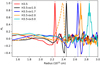 |
Fig. 24. Auto-correlation function (see Eq. (20)) of the radial velocities at the location of the composition interfaces (dotted vertical lines) at the end of the simulations for the 3.5 M⊙ models. The black dashed line shows the auto-correlation function at the Schwarzschild boundary of model H3.5-ov2.0. |
At this point we can also check whether our rms velocities fulfil the scaling relation  predicted by MLT. We find that our simulations in the analysed mass range agree fairly well with this scaling relation (see Fig. 25). However, the spread in
  for a given luminosity is much larger than expected. Models with the same stellar mass have a similar luminosity, but the mass of the convective core is quite different due to the self-consistent evolution of the one-dimensional models including overshooting (see Col. 5 in Tables 1 and 2). This suggests that second order effects like the mass of a CZ, or respectively its size, should also be considered in velocity estimates.
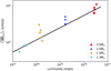 |
Fig. 25. Time-averaged convective velocities as a function of stellar luminosity. The predicted MLT scaling is shown by the black line. |
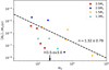 |
Fig. 26. Time-averaged mass entrainment rate as a function of the bulk Richardson number for all our models. Each symbol corresponds to a different model. The black dashed line represents an entrainment law according to Eq. (17) with n = 1.32. |
We find that the convective boundaries of our models have bulk Richardson numbers in the range 600 < Rib < 55 000, which is comparable to the unenhanced luminosity simulation in Cristini et al. (2019). Combining these values with the mixing rates in Tables 1 and 2 we are able to fit an entrainment law to our simulations. This fit gives n = 1.32 ± 0.79 and A = 4 ⋅ 10−2. Even though this is in agreement with the theoretical prediction n = 1 by Linden (1975) we would argue that the large error in the fit actually suggests that (1) our simulations should not be fitted by a single universal entrainment law, and that (2) they indicate that the entrainment law does not only depend on Rib. One possible extension to the entrainment law would be to include the Peclet number in the analysis as it was proposed by Noh & Fernando (1993). Obviously, further research is required to analyse the different influences on the entrainment process.
5. Conclusion
We presented a total of 21 two-dimensional simulations of convective cores in ZAMS stars ranging from 1.3 to 3.5 M⊙. The simulation domain covers the convective core and a large fraction of the convectively stable layer on top of it. Due to the pseudo incompressible approximation of Maestro, we were able to follow the convective flow for many convective turnover times at the nominal stellar luminosity, which allowed us to study the time evolution of the very low Mach number flows and their mixing across the convective core boundary in detail. By comparing a simulation that resolves high frequency IGW in time with one that only resolves the advection timescale we determined that high frequency IGW do not play a significant role in the mixing, and therefore decided to not fully resolve them in time. This allowed us to increase the numerical timestep further, and hence to simulate more than 100 convective turnover times in most of our simulations. In order to guarantee the accuracy of simulations using large timesteps, we replaced the advection scheme in the time integrator of Maestro with a 4th order Runge-Kutta scheme, which reduces the amplitude of numerical artefacts in the convectively stable layer.
We used Garstec one-dimensional stellar evolution models with a solar-like composition as input for our hydrodynamic simulations. During the mapping procedure from one-dimensional to two-dimensional we preserved the thermal stratification of the one-dimensional model following Edelmann et al. (2017), which reduced the influence of the transient phase due to thermal readjustments at the beginning of the simulations. We analysed the time evolution of the convective boundary in detail and identified three fundamental types of boundary definitions. We showed that for main-sequence convection dynamic (defined by the flow velocity) and structural (defined by the temperature stratification) boundaries remain mostly constant for the simulated timescales but at different radial locations. In contrast, the chemical boundary (defined by the composition) evolves in time, demonstrating the effects of mixing. While the time evolution of the chemical boundary indicates that mixing is slowing down with time, we were not able to simulate long enough to establish an equilibrium state. In order to estimate the maximum extent of the mixed region around a convective core we therefore used a series of one-dimensional models computed with increasing values of the overshooting parameter fov.
We found that increasing fov in the initial model reduces the mixing rate of hydrogen into the convective core. Furthermore, increasing fov beyond a certain limiting value leads to an abrupt change in the mixing characteristics, namely from a continuous entrainment process to an episodic mixing behaviour. We attribute this change to an increasing influence of diffusive mixing due to IGW and of numerics as the distance between the composition interface and the Schwarzschild boundary of the convective core increases.
We measured the diffusion coefficients of the flow with tracer particles, and we found that the results within the CZ and in the immediate surrounding of it are well converged in our simulations. However, this is not the case further away from the convective boundary, where the estimated diffusion coefficients are orders of magnitude smaller than in the CZ. On the one hand, the clear separation of these two regions hints that the overshooting description itself has to be altered to account for different mixing processes. On the other hand, comparing our results with asteroseismic constraints we argue that the contribution of diffusive mixing is largely overestimated in our simulations, which means that the simulations that are dominated by diffusion would show even smaller mixing rates in a higher resolved simulation. This allows us to constrain fov to values where no episodic mixing can be seen in our simulations.
With this procedure we determined fov to be in the range 0.01 < fov < 0.017 in a 3.5 M⊙ star, which is in rough agreement with empirical estimates. Reducing the simulated stellar mass and therefore the size of the convective core shows that the tight connection between fov and the pressure scale height requires a reduction of fov used on the main-sequence towards lower stellar masses, for example we could limit fov in a 1.3 M⊙ star with a tiny convective core to fov < 0.005. This result confirms findings when comparing isochrones with open cluster observations (e.g., Pietrinferni et al. 2004; Magic et al. 2010) and it agrees with results using eclipsing binaries (Claret & Torres 2016). In particular, we find that our overshooting estimates are in good agreement with asteroseismic observations of γ Dor stars by Mombarg et al. (2019).
Practically limiting the overshooting can be achieved by a mass dependent overshooting parameter or by geometrically limiting the overshooting region based on the size of the convective region itself, where the latter is the physically more relevant property. However, the exact functional form remains to be determined.
Moreover, we find that models with large values of fov develop a thin penetration region where the temperature gradient lies between the radiative and the adiabatic gradient as it was predicted by, for example van Ballegooijen (1982) and Zahn (1991). In models with small fov values this effect is probably masked by changes in the molecular gradient due to the strong chemical mixing in these simulations. Nevertheless, it is not possible to estimate the maximum extent of the penetration region in any of our simulations, since we are not able to simulate the relevant thermal timescales.
We also investigated the possibility to describe chemical mixing in the form of an entrainment law as proposed by Meakin & Arnett (2007). We were not able to find an acceptable universal fit that covers all stellar masses in this work, indicating that entrainment laws need to include more parameters as they currently do.
Three-dimensional simulations are needed to confirm these results. Initial tests in Higl (2019) point in this direction, but computational limits regarding the numerical stability of the convectively stable layer in these simulations currently prevent us from making conclusive statements. Proposed well-balancing methods (see e.g., Berberich et al. 2019) could potentially help to provide these answers in the future.
Acknowledgments
The J. H. would like to thank M. Zingale for fruitful discussion on the numerics of Maestro. The E3.5 simulation and most of the diffusion coefficient analysis has been computed on the Hydra and Draco clusters at the Max Planck Computing and Data Facility (MPCDF). J. H. acknowledges support by the Klaus Tschira Foundation. This work made use of the Matplotlib (Hunter 2007) package and used MPI4Py (Dalcin et al. 2011) for parallel data processing.
References
- Aerts, C., Christensen-Dalsgaard, J., & Kurtz, D. W. 2010, Asteroseismology (Springer Science+Business Media B.V.) [Google Scholar]
- Aerts, C., Mathis, S., & Rogers, T. 2019, ARA&A, 57, 35 [NASA ADS] [CrossRef] [MathSciNet] [Google Scholar]
- Almgren, A. S., Bell, J. B., Rendleman, C. A., & Zingale, M. 2006a, ApJ, 637, 922 [Google Scholar]
- Almgren, A. S., Bell, J. B., Rendleman, C. A., & Zingale, M. 2006b, ApJ, 649, 927 [Google Scholar]
- Almgren, A. S., Bell, J. B., Nonaka, A., & Zingale, M. 2008, ApJ, 684, 449 [Google Scholar]
- Andrassy, R., Herwig, F., Woodward, P., & Ritter, C. 2020, MNRAS, 491, 972 [Google Scholar]
- Angelou, G. C., Bellinger, E. P., Hekker, S., et al. 2020, MNRAS, 493, 4987 [Google Scholar]
- Aparicio, A., Bertelli, G., Chiosi, C., & Garcia-Pelayo, J. M. 1990, A&A, 240, 262 [Google Scholar]
- Batchelor, G. K. 1969, Phys. Fluids, 12, II [Google Scholar]
- Battino, U., Pignatari, M., Ritter, C., et al. 2016, ApJ, 827, 30 [Google Scholar]
- Bell, J. B., Day, M. S., Almgren, A. S., Lijewski, M. J., & Rendleman, C. A. 2002, Int. J. Numer. Methods Fluids, 40, 209 [Google Scholar]
- Berberich, J. P., Chandrashekar, P., & Klingenberg, C. 2019, ArXiv e-prints [arXiv:1903.05154] [Google Scholar]
- Bertelli, G., Bressan, A., & Chiosi, C. 1992, ApJ, 392, 522 [Google Scholar]
- Böhm-Vitense, E. 1958, Z. Astrophys., 46, 108 [Google Scholar]
- Bowman, D. M., Aerts, C., Johnston, C., et al. 2019, A&A, 621, A135 [NASA ADS] [CrossRef] [EDP Sciences] [Google Scholar]
- Brummell, N. H., Clune, T. L., & Toomre, J. 2002, ApJ, 570, 825 [Google Scholar]
- Christy, R. F. 1966, ApJ, 144, 108 [Google Scholar]
- Claret, A., & Torres, G. 2016, A&A, 592, A15 [NASA ADS] [CrossRef] [EDP Sciences] [Google Scholar]
- Constantino, T., & Baraffe, I. 2018, A&A, 618, A177 [NASA ADS] [CrossRef] [EDP Sciences] [Google Scholar]
- Couston, L.-A., Lecoanet, D., Favier, B., & Le Bars, M. 2018, Phys. Rev. Lett., 120, 244505 [Google Scholar]
- Cristini, A., Meakin, C., Hirschi, R., et al. 2017, MNRAS, 471, 279 [Google Scholar]
- Cristini, A., Hirschi, R., Meakin, C., et al. 2019, MNRAS, 484, 4645 [Google Scholar]
- Dalcin, L. D., Paz, R. R., Kler, P. A., & Cosimo, A. 2011, Adv. Water Resour., 34, 1124 [Google Scholar]
- Deheuvels, S., Brandão, I., Silva Aguirre, V., et al. 2016, A&A, 589, A93 [NASA ADS] [CrossRef] [EDP Sciences] [Google Scholar]
- Durran, D. R. 1989, J. Atmos. Sci., 46, 1453 [Google Scholar]
- Edelmann, P. V. F., Röpke, F. K., Hirschi, R., Georgy, C., & Jones, S. 2017, A&A, 604, A25 [NASA ADS] [CrossRef] [EDP Sciences] [Google Scholar]
- Edelmann, P. V. F., Ratnasingam, R. P., Pedersen, M. G., et al. 2019, ApJ, 876, 4 [Google Scholar]
- Freytag, B., Ludwig, H.-G., & Steffen, M. 1996, A&A, 313, 497 [Google Scholar]
- Gilet, C. E. 2012, PhD Thesis, University of California, Berkeley, USA [Google Scholar]
- Gilet, C., Almgren, A. S., Bell, J. B., et al. 2013, ApJ, 773, 137 [Google Scholar]
- Herwig, F., Freytag, B., Fuchs, T., et al. 2007, in Why Galaxies Care About AGB Stars: Their Importance as Actors and Probes, eds. F. Kerschbaum, C. Charbonnel, R. F. Wing, et al., ASP Conf. Ser., 378, 43 [Google Scholar]
- Higl, J. 2019, PhD Thesis, Technische Universität München, Germany [Google Scholar]
- Higl, J., & Weiss, A. 2017, A&A, 608, A62 [NASA ADS] [CrossRef] [EDP Sciences] [Google Scholar]
- Higl, J., Siess, L., Weiss, A., & Ritter, H. 2018, A&A, 617, A36 [NASA ADS] [CrossRef] [EDP Sciences] [Google Scholar]
- Horst, L., Edelmann, P. V. F., Andrassy, R., et al. 2020, A&A, 641, A18 [CrossRef] [EDP Sciences] [Google Scholar]
- Hunter, J. D. 2007, Comput. Sci. Eng., 9, 90 [NASA ADS] [CrossRef] [Google Scholar]
- Iben, I. Jr. 1975, ApJ, 196, 525 [Google Scholar]
- Jacobs, A. M., Zingale, M., Nonaka, A., Almgren, A. S., & Bell, J. B. 2016, ApJ, 827, 84 [Google Scholar]
- Jones, S., Andrassy, R., Sandalski, S., et al. 2017, MNRAS, 465, 2991 [Google Scholar]
- Jørgensen, A. C. S., Mosumgaard, J. R., Weiss, A., Silva Aguirre, V., & Christensen-Dalsgaard, J. 2018, MNRAS, 481, L35 [Google Scholar]
- Kercek, A., Hillebrandt, W., & Truran, J. W. 1998, A&A, 337, 379 [NASA ADS] [Google Scholar]
- Kippenhahn, R., Weigert, A., & Weiss, A. 2012, Stellar Struct. Evol., [Google Scholar]
- Korre, L., Garaud, P., & Brummell, N. H. 2019, MNRAS, 484, 1220 [NASA ADS] [CrossRef] [Google Scholar]
- Kraichnan, R. H. 1967, Physics of Fluids, 10, 1417 [Google Scholar]
- Lattanzio, J. C., Tout, C. A., Neumerzhitckii, E. V., Karakas, A. I., & Lesaffre, P. 2017, Mem. Soc. Astron. It., 88, 248 [Google Scholar]
- Lecoanet, D., Brown, B. P., Zweibel, E. G., et al. 2014, ApJ, 797, 94 [Google Scholar]
- Li, Y. 2017, ApJ, 841, 10 [Google Scholar]
- Linden, P. F. 1975, J. Fluid Mech., 71, 385 [Google Scholar]
- Magic, Z., Serenelli, A., Weiss, A., & Chaboyer, B. 2010, ApJ, 718, 1378 [Google Scholar]
- Magic, Z., Collet, R., Asplund, M., et al. 2013, A&A, 557, A26 [NASA ADS] [CrossRef] [EDP Sciences] [Google Scholar]
- Meakin, C. A., & Arnett, D. 2007, ApJ, 667, 448 [Google Scholar]
- Mellado, J. P. 2017, Ann. Rev. Fluid Mech., 49, 145 [Google Scholar]
- Michielsen, M., Pedersen, M. G., Augustson, K. C., Mathis, S., & Aerts, C. 2019, A&A, 628, A76 [NASA ADS] [CrossRef] [EDP Sciences] [Google Scholar]
- Miczek, F., Röpke, F. K., & Edelmann, P. V. F. 2015, A&A, 576, A50 [NASA ADS] [CrossRef] [EDP Sciences] [Google Scholar]
- Mocák, M., Müller, E., Weiss, A., & Kifonidis, K. 2009, A&A, 501, 659 [NASA ADS] [CrossRef] [EDP Sciences] [Google Scholar]
- Mombarg, J. S. G., Van Reeth, T., Pedersen, M. G., et al. 2019, MNRAS, 485, 3248 [Google Scholar]
- Moravveji, E., Townsend, R. H. D., Aerts, C., & Mathis, S. 2016, ApJ, 823, 130 [Google Scholar]
- Mosumgaard, J. R., Jørgensen, A. C. S., Weiss, A., Silva Aguirre, V., & Christensen-Dalsgaard, J. 2020, MNRAS, 491, 1160 [Google Scholar]
- Noh, Y., & Fernando, H. J. 1993, Dyn. Atmos. Oceans, 17, 187 [Google Scholar]
- Nonaka, A., Almgren, A. S., Bell, J. B., et al. 2010, ApJS, 188, 358 [Google Scholar]
- Pedersen, M. G., Aerts, C., Pápics, P. I., & Rogers, T. M. 2018, A&A, 614, A128 [NASA ADS] [CrossRef] [EDP Sciences] [Google Scholar]
- Pietrinferni, A., Cassisi, S., Salaris, M., & Castelli, F. 2004, ApJ, 612, 168 [NASA ADS] [CrossRef] [Google Scholar]
- Pols, O. R., Tout, C. A., Schroder, K.-P., Eggleton, P. P., & Manners, J. 1997, MNRAS, 289, 869 [Google Scholar]
- Pratt, J., Baraffe, I., Goffrey, T., et al. 2016, A&A, 593, A121 [NASA ADS] [CrossRef] [EDP Sciences] [Google Scholar]
- Pratt, J., Baraffe, I., Goffrey, T., et al. 2017, A&A, 604, A125 [NASA ADS] [CrossRef] [EDP Sciences] [Google Scholar]
- Pratt, J., Baraffe, I., Goffrey, T., et al. 2020, A&A, 638, A15 [CrossRef] [EDP Sciences] [Google Scholar]
- Ribas, I., Jordi, C., & Giménez, Á. 2000, MNRAS, 318, L55 [Google Scholar]
- Robinson, F. J., Demarque, P., Li, L. H., et al. 2003, MNRAS, 340, 923 [Google Scholar]
- Rogers, T. M. 2015, ApJ, 815, L30 [Google Scholar]
- Rogers, T. M., & McElwaine, J. N. 2017, ApJ, 848, L1 [Google Scholar]
- Rogers, T. M., Lin, D. N. C., McElwaine, J. N., & Lau, H. H. B. 2013, ApJ, 772, 21 [Google Scholar]
- Stancliffe, R. J., Fossati, L., Passy, J. C., & Schneider, F. R. N. 2015, A&A, 575, A117 [NASA ADS] [CrossRef] [EDP Sciences] [Google Scholar]
- Staritsin, E. I. 2013, Astron. Rep., 57, 380 [Google Scholar]
- Stevens, B. 2002, QJRAS, 128, 2663 [Google Scholar]
- Sutherland, B. R. 2010, Internal Gravity Waves (Cambridge University Press) [CrossRef] [Google Scholar]
- Timmes, F. X. 2000, ApJ, 528, 913 [Google Scholar]
- Timmes, F. X., & Swesty, F. D. 2000, ApJS, 126, 501 [Google Scholar]
- Turk, M. J., Smith, B. D., Oishi, J. S., et al. 2011, ApJS, 192, 9 [Google Scholar]
- Turner, J. S. 1986, J. Fluid Mech., 173, 431 [Google Scholar]
- Valle, G., Dell’Omodarme, M., Prada Moroni, P. G., & Degl’Innocenti, S. 2016, A&A, 587, A16 [NASA ADS] [CrossRef] [EDP Sciences] [Google Scholar]
- van Ballegooijen, A. A. 1982, A&A, 113, 99 [NASA ADS] [Google Scholar]
- VandenBerg, D. A., Bergbusch, P. A., & Dowler, P. D. 2006, ApJS, 162, 375 [Google Scholar]
- Vasil, G. M., Lecoanet, D., Brown, B. P., Wood, T. S., & Zweibel, E. G. 2013, ApJ, 773, 169 [Google Scholar]
- Viallet, M., Meakin, C., Arnett, D., & Mocák, M. 2013, ApJ, 769, 1 [Google Scholar]
- Wagstaff, G., Miller Bertolami, M. M., & Weiss, A. 2020, MNRAS, 493, 4748 [Google Scholar]
- Weaver, T. A., Zimmerman, G. B., & Woosley, S. E. 1978, ApJ, 225, 1021 [Google Scholar]
- Weiss, A., & Schlattl, H. 2008, Ap&SS, 316, 99 [Google Scholar]
- Yang, W. 2016, ApJ, 829, 68 [Google Scholar]
- Zahn, J. P. 1991, A&A, 252, 179 [Google Scholar]
- Zingale, M., Almgren, A. S., Bell, J. B., Nonaka, A., & Woosley, S. E. 2009, ApJ, 704, 196 [Google Scholar]
All Tables
Overview of our two-dimensional simulations of main-sequence stars of different masses.
All Figures
|
Fig. 1. Flow chart of the modified time advancement algorithm. The computed or updated quantities of each sub step are given in blue. |
| In the text | |
|
Fig. 2. Horizontally averaged profiles of a constructed stable atmosphere. The black solid line shows the initial N2 profile. Red lines give the velocity magnitude profile after 3 105 s for the predictor-corrector scheme (dashed) and the Runge-Kutta integrator (solid), respectively. |
| In the text | |
|
Fig. 3. Initial density (black) and superadiabaticity (red) of the model H3.5 (solid; see Table 1) and H3.5-T (dotted), respectively. Dashed lines give the stratification as predicted by Garstec. The vertical dashed and dotted lines indicate the boundary of the convective core and of the computational domain, respectively. In the shaded region we damp the velocities. |
| In the text | |
|
Fig. 4. Evolution of the density-averaged convective velocity magnitude |
| In the text | |
|
Fig. 5. Velocity magnitude (left panels) and deviations of the hydrogen mass fraction from its angulary averaged value X′(x, y) = X(x, y)−⟨X⟩(r) (right panels) of simulation H3.5, H3.5-ov1.7, and H3.5-ov3.0 (from top to bottom) after 2 107 s. The magenta dashed circles mark the initial size of the mixed core, while the black dashed circles show the size of the convective core according to the Schwarzschild criterion. The streamlines in the left panels indicate the flow direction. |
| In the text | |
|
Fig. 6. Time-averaged velocity profiles for different two-dimensional simulations of a 3.5 M⊙ star. The averages extend from 5 106 s to 107 s. The dashed black line shows, scaled up by a factor of 10, the velocity profile predicted by MLT. |
| In the text | |
|
Fig. 7. Various radial profiles in the neigbourhood of the convective boundary. ⟨⟨Uϕ⟩⟩t, ⟨⟨Ekin⟩⟩t, and ⟨⟨∇ex⟩⟩t are the combined spatial (indicated by ⟨.⟩) and time (⟨.⟩t) averages of the angular velocity Uϕ, the kinetic energy Ekin, and the superadiabaticity ∇ex = ∇mlt − ∇ad, respectively. The time averages are taken from 1.82 108 s to 2.06 108 s using 100 output files from the H3.5 simulation. ⟨σ(Ekin)⟩t is the time-averaged standard deviation of the kinetic energy (see Eq. (14)). The angularly averaged hydrogen mass fraction profile ⟨X⟩ is taken at 2.06 108 s. The curves of ⟨⟨Uϕ⟩⟩t, ⟨⟨Ekin⟩⟩t, ⟨⟨∇ex⟩⟩t, and ⟨σ(Ekin)⟩t are normalized to the values corresponding to their respective boundary definitions (see text), which means that the black dotted line indicates the boundary values of each line. The dashed vertical lines mark the radial locations of our favoured boundaries. |
| In the text | |
|
Fig. 8. Temporal evolution of the various convective boundary locations (see text) in the H3.5 simulation. |
| In the text | |
|
Fig. 9. Temperature fluctuations around the angularly average value in the H3.5 simulation at 8 107 s. |
| In the text | |
|
Fig. 10. Distribution of tracer particles for model H3.5 at several epochs. We show only 4000 of the 40 000 tracer particles used in the simulation, which are coloured according to their initial radial location given in the upper left panel. |
| In the text | |
|
Fig. 11. Radial diffusion coefficients estimated from the advection of 40 000 tracer particles followed for 1.5 106 s for models of different grid size. The dashed and dotted lines labelled ‘H3.5 – 1.6e5’ and ‘H3.5 – 1.0e6’ represent the same quantity but evaluated with 160 000 and 106 tracer particles in model H3.5, respectively. The dashed vertical line indicates Rdyn of model H3.5. |
| In the text | |
|
Fig. 12. Time evolution of the mean squared radial displacement of tracer particles in model H3.5. The particles which where used for the analysis were taken at r = 2.5 106 cm, 3.0 106 cm, and 4.0 106 cm. Stars, diamonds, and crosses correspond to analysis runs with a total of 40 000, 160 000, and 106 tracer particles, respectively. |
| In the text | |
|
Fig. 13. Change in the hydrogen mass for the initial convective core of our 3.5 M⊙ simulations. The top and bottom panels show the hydrogen mass relative to its initial value and the corresponding rate of change, respectively. |
| In the text | |
|
Fig. 14. Same as Fig. 13, but for simulations performed with different fov values. The vertical dashed line indicates t = 2 107 s. |
| In the text | |
|
Fig. 15. Illustration of our overshooting calibration method (see text). |
| In the text | |
|
Fig. 16. Radial diffusion coefficients estimated from 40 000 tracer particles over 2.5 106 s for the models with different initial values of fov. The lines have been shifted such that the radial position of the structural boundary matches for all the simulations. The dotted vertical lines indicate the position of Rchem in each run. The red dashed line shows D according to Eq. (11) with fov = 0.01 |
| In the text | |
|
Fig. 17. Comparison of the different ways to compute the superadiabaticity ∇ex in Maestro simulations (see text for more details). Shown are angularly averaged profiles from model H3.5 at 108 s. |
| In the text | |
|
Fig. 18. Angularly averaged profiles of the superadiabaticity in models of a 3.5 M⊙ star with different amounts of overshooting. Dashed and solid lines show profiles according to the Schwarzschild criterion at t = 0 and after 4 107 s, respectively. The dotted lines give the initial profiles according to the Ledoux criterion. |
| In the text | |
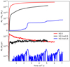 |
Fig. 19. Same as Fig. 13, but for a 2.0 M⊙ star. |
| In the text | |
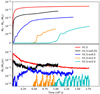 |
Fig. 20. Same as Fig. 13, but for a 1.5 M⊙ star. |
| In the text | |
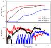 |
Fig. 21. Same as Fig. 13, but for a 1.3 M⊙ star. |
| In the text | |
|
Fig. 22. Colour plot of the evolution of angularly averaged velocity magnitude profiles in model H1.3 during a timespan of 1.3 108 s. The radial position of the initial Schwarzschild boundary and the propagation direction of IGWs are marked by white and black dashed lines, respectively. |
| In the text | |
|
Fig. 23. Convectively mixed core mass for models with (black dots) and without overshooting (black stars) on the ZAMS. Blue and green ellipses show the same quantity, but using a geometrical cutoff for the overshooting and observational constraints by Mombarg et al. (2019), respectively. The red triangles denote the derived upper limits from our simulations. The black cross indicates the size of the mixed core of a 2.0 M⊙ star close to the end of its main-sequence evolution when the model is computed without overshooting. |
| In the text | |
|
Fig. 24. Auto-correlation function (see Eq. (20)) of the radial velocities at the location of the composition interfaces (dotted vertical lines) at the end of the simulations for the 3.5 M⊙ models. The black dashed line shows the auto-correlation function at the Schwarzschild boundary of model H3.5-ov2.0. |
| In the text | |
|
Fig. 25. Time-averaged convective velocities as a function of stellar luminosity. The predicted MLT scaling is shown by the black line. |
| In the text | |
|
Fig. 26. Time-averaged mass entrainment rate as a function of the bulk Richardson number for all our models. Each symbol corresponds to a different model. The black dashed line represents an entrainment law according to Eq. (17) with n = 1.32. |
| In the text | |
Current usage metrics show cumulative count of Article Views (full-text article views including HTML views, PDF and ePub downloads, according to the available data) and Abstracts Views on Vision4Press platform.
Data correspond to usage on the plateform after 2015. The current usage metrics is available 48-96 hours after online publication and is updated daily on week days.
Initial download of the metrics may take a while.