| Issue |
A&A
Volume 645, January 2021
|
|
|---|---|---|
| Article Number | L12 | |
| Number of page(s) | 7 | |
| Section | Letters to the Editor | |
| DOI | https://doi.org/10.1051/0004-6361/202039966 | |
| Published online | 26 January 2021 | |
Letter to the Editor
Downflowing umbral flashes as evidence of standing waves in sunspot umbrae
1
Instituto de Astrofísica de Canarias, 38205 C/ Vía Láctea, s/n, La Laguna, Tenerife, Spain
e-mail: This email address is being protected from spambots. You need JavaScript enabled to view it.
2
Departamento de Astrofísica, Universidad de La Laguna, 38205 La Laguna, Tenerife, Spain
3
Institute of Theoretical Astrophysics, University of Oslo, PO Box 1029 Blindern, 0315 Oslo, Norway
4
Rosseland Centre for Solar Physics, University of Oslo, PO Box 1029 Blindern, 0315 Oslo, Norway
5
Institute for Solar Physics, Dept. of Astronomy, Stockholm University, AlbaNova University Centre, 10691 Stockholm, Sweden
Received:
23
November
2020
Accepted:
6
January
2021
Abstract
Context. Umbral flashes are sudden brightenings commonly visible in the core of some chromospheric lines. Theoretical and numerical modeling suggests that they are produced by the propagation of shock waves. According to these models and early observations, umbral flashes are associated with upflows. However, recent studies have reported umbral flashes in downflowing atmospheres.
Aims. We aim to understand the origin of downflowing umbral flashes. We explore how the existence of standing waves in the umbral chromosphere impacts the generation of flashed profiles.
Methods. We performed numerical simulations of wave propagation in a sunspot umbra with the code MANCHA. The Stokes profiles of the Ca II 8542 Å line were synthesized with the NICOLE code.
Results. For freely propagating waves, the chromospheric temperature enhancements of the oscillations are in phase with velocity upflows. In this case, the intensity core of the Ca II 8542 Å atmosphere is heated during the upflowing stage of the oscillation. However, a different scenario with a resonant cavity produced by the sharp temperature gradient of the transition region leads to chromospheric standing oscillations. In this situation, temperature fluctuations are shifted backward and temperature enhancements partially coincide with the downflowing stage of the oscillation. In umbral flash events produced by standing oscillations, the reversal of the emission feature is produced when the oscillation is downflowing. The chromospheric temperature keeps increasing while the atmosphere is changing from a downflow to an upflow. During the appearance of flashed Ca II 8542 Å cores, the atmosphere is upflowing most of the time, and only 38% of the flashed profiles are associated with downflows.
Conclusions. We find a scenario that remarkably explains the recent empirical findings of downflowing umbral flashes as a natural consequence of the presence of standing oscillations above sunspot umbrae.
Key words: methods: numerical / Sun: chromosphere / Sun: oscillations / sunspots / techniques: polarimetric
© ESO 2021
1. Introduction
Oscillations are a ubiquitous phenomenon in the Sun. Their signatures have been detected almost everywhere, from the solar interior to the outer atmosphere. One of the most spectacular manifestations of solar oscillations are umbral flashes (UFs). They were discovered by Beckers & Tallant (1969; see also Wittmann 1969), who observed them in sunspot umbrae as periodic brightness enhancements in the core of some chromospheric spectral lines. Following their first detection, UFs were associated with magneto-acoustic wave propagation in umbral atmospheres (Beckers & Tallant 1969), and soon after Havnes (1970) suggested that UFs in Ca II lines were formed due to the temperature enhancement during the compressional stage of these waves.
The analysis of spectropolarimetric data has become a common approach in the study of UFs over the last two decades, since the studies undertaken by Socas-Navarro et al. (2000a,b). They found anomalous polarization in the Stokes profiles and interpreted it as indirect evidence of very fine structure in UFs, unresolved in arc-second resolution observations. Their model had one hot upflowing component embedded in a cool downflowing medium. Further independent, but still indirect, evidence of such fine structure was obtained by Centeno et al. (2005). Subsequent studies, benefiting from observations acquired with higher spatio-temporal resolution, were able to resolve those components in imaging observations (Socas-Navarro et al. 2009; Henriques & Kiselman 2013; Bharti et al. 2013; Yurchyshyn et al. 2014; Henriques et al. 2015) and in full spectropolarimetric observations (Rouppe van der Voort & de la Cruz Rodríguez 2013; de la Cruz Rodríguez et al. 2013; Nelson et al. 2017). Nonlocal thermodynamical equilibrium (NLTE) inversions of Ca II 8542 Å sunspot observations using the NICOLE code (Socas-Navarro et al. 2015) have found that UF atmospheres are associated with temperature increments of around 1000 K and strong upflows (de la Cruz Rodríguez et al. 2013). These observational measurements exhibit a good agreement with the theoretical picture of UFs as a manifestation of upward propagating slow magneto-acoustic waves. The amplitude of these waves increases with height as a result of the density stratification, leading to the development of chromospheric shocks (Centeno et al. 2006; Felipe et al. 2010a) and UFs (Bard & Carlsson 2010; Felipe et al. 2014). The properties of those UF shocks have recently been evaluated by interpreting spectropolarimetric observations with the support of the Rankine-Hugoniot relations (Anan et al. 2019; Houston et al. 2020).
The first NLTE inversions of UFs (Socas-Navarro et al. 2001) were computationally very expensive (typically several hours per individual spectrum), and therefore only a few profiles from the same location and different times were inverted. Later improvements in code optimization, parallelization, and computer hardware allowed de la Cruz Rodríguez et al. (2013) to analyze a few 2D maps with spatial resolution. As this trend continued, it is now possible to make UF studies with higher spatial and temporal resolution and much better statistics (e.g., Henriques et al. 2017; Joshi & de la Cruz Rodríguez 2018; Houston et al. 2018, 2020). These recent results have revealed the existence of UFs whose Stokes profiles are better reproduced with atmospheres dominated by downflows (Henriques et al. 2017; Bose et al. 2019; Houston et al. 2020).
Accommodating the downflowing UFs in the widely accepted scenario of upward propagating shock waves is a theoretical challenge. Studies employing sophisticated synthesis tools and numerical simulations of the umbral atmosphere have validated the upflowing UF model (Bard & Carlsson 2010; Felipe et al. 2014, 2018a; Felipe & Esteban Pozuelo 2019). In those simulations, magneto-acoustic waves can propagate from the photosphere to the chromosphere. According to the phase relations of these propagating waves, velocity and temperature oscillations exhibit opposite phases (considering that positive velocities correspond to downflows), and the temperature increase responsible for the flash matches an upflow. However, recent studies have shown evidence of a resonant cavity above sunspot umbrae (see Jess et al. 2020a,b; Felipe 2021; Felipe et al. 2020). This cavity is produced by wave reflections at the strong temperature gradient in the transition region (e.g., Zhugzhda & Locans 1981; Zhugzhda 2008). Waves trapped in a resonant cavity produce standing oscillations whose temperature fluctuations are delayed by a quarter period with respect to the velocity signal, instead of the half-period delay from freely propagating waves (Deubner 1974; Felipe et al. 2020). In this study, we use numerical simulations and full-Stokes NLTE radiative transfer calculations to explore the generation of intensity emission cores in the Ca II 8542 Å line during the downflowing stage of standing umbral oscillations, as well as how they can support the existence of the recently reported downflowing UFs.
2. Numerical methods
Nonlinear wave propagation between the solar interior and the corona was simulated using the code MANCHA (Khomenko & Collados 2006; Felipe et al. 2010b) in a 2D domain. The details of the simulations can be found in Appendix A. We computed synthetic full-Stokes spectra in the Ca II 8542 Å line taking snapshots from our numerical simulation and then computing the spectra with the NICOLE code (Socas-Navarro et al. 2015, see details in Appendix B). The code assumes statistical equilibrium. Wedemeyer-Böhm & Carlsson (2011) showed that nonequilibrium effects in Ca II are small at the formation height of the infrared triplet lines, and, therefore, statistical equilibrium should suffice to model Ca II atoms. We calculated the transition probabilities between levels for Ca II in a sunspot model. They indicate characteristic transition times much shorter than one second (Appendix B), meaning that departures from statistical equilibrium are insignificant for the dynamics studied here.
3. Results
We analyzed how UFs are generated in the case of propagating and standing oscillations. In Appendix C, we discuss the differences in the phase relations between temperature and velocity fluctuations from propagating and standing waves as determined from the analysis of numerical simulations. In the following, for the examination of the propagating-wave case, we focus on the first wavefront of the simulation reaching the chromosphere, before any previous wavefronts are reflected and a standing wave is settled. We chose to follow this approach (instead of using an independent simulation without transition region) in order to employ exactly the same atmospheric stratification for both cases. This way, we can ensure that the differences in the properties of the UFs are produced by the nature of the oscillations and not by the changes in the background atmospheres.
3.1. Umbral flashes from propagating waves
Figure 1 illustrates the development of UFs generated by a propagating wave at the beginning of the simulation. This case is qualitatively comparable to the synthetic UFs analyzed by Bard & Carlsson (2010), Felipe et al. (2014, 2018a), and Felipe & Esteban Pozuelo (2019). We refer the reader to those papers for a detailed discussion of the formation of UFs. In the present paper, we focus on evaluating the chromospheric plasma motions during the appearance of the UF. Similarly to Henriques et al. (2017), we define a profile as “flashed” when the intensity around the core of the Ca II 8542 Å line is above the value of Stokes I at Δλ = 0.942 Å.
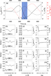 |
Fig. 1. Development of a UF produced by propagating waves as seen in Ca II 8542 Å. Panel a: temporal evolution of the vertical velocity (solid line, left axis), temperature (dashed black line, black right axis), and density (dashed red line, red right axis) fluctuations at z = 1.35 Mm. The blue shaded region corresponds to the time when a UF is identified in the Stokes profiles and the atmosphere is upflowing at log τ = −5.1. Lower panels: stokes I (left column), Stokes V (middle column), and atmospheric models (right column). Each row corresponds to a different time step, as indicated at the bottom of the first column panels and the vertical dotted lines in panel a. In the right column, the vertical velocity (solid line, left axis) and temperature (dashed line, right axis) of the atmospheric model is plotted. The vertical dashed line marks the height of log τ = −5.1. |
The time steps when flashed profiles take place are marked in blue in Fig. 1a. As expected, they coincide with a temperature enhancement at z = 1.35 Mm, which is roughly the height where the response of the Ca II 8542 Å line to temperature is at its maximum during UFs (Fig. A.1). The temperature maximum precedes the highest value of the upflow velocity by 9 s. Prior to the appearance of the flash (Fig. 1b), the atmosphere is downflowing, in accordance with observations (Henriques et al. 2020), but the temperature fluctuation is too low to produce an emission core (panel d). When the UF starts to develop (panel e), the atmosphere is upflowing at the optical depth where the response of the line is at its maximum (log τ ≈ −5.1, Fig. A.1) and is downflowing at higher layers (panel g). A similar situation can be seen at later steps (panels h and j). The change from upflows to downflows at a certain height is a manifestation of the propagating character of the waves since, for standing waves, we expect most of the chromosphere to be oscillating in phase.
3.2. Umbral flashes from standing waves
The atmospheres generating UFs in the case of standing oscillations exhibit several significant differences from those of propagating waves. First, as discussed in Appendix C, the phase shift between velocity and temperature fluctuations is different. In the UF illustrated in Fig. 2, the peak of the temperature enhancement at z = 1.35 Mm takes place 26 s before the maximum value of the upflow velocity (panel a). Second, higher chromospheric layers are oscillating in phase above the resonant node as a result of the standing oscillations (right column in the bottom subset of Fig. 2).
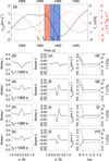 |
Fig. 2. Same as Fig. 1, but for standing oscillations. The red shaded region in panel a indicates the time when a UF is identified in the Stokes profiles and the atmosphere is downflowing at log τ = −5.1. |
Due to the earlier appearance of a positive temperature fluctuation (relative to the case of propagating waves), temperature enhancements partially coincide with the downflow of the velocity oscillation. This way, chromospheric temperatures high enough to generate UFs are reached while a strong downflow is still taking place (panels e–g from Fig. 2). The strongest UF (at the peak of the temperature fluctuation) is found when the chromosphere is already upflowing (panels h–j from Fig. 2). In this example, the total duration of the UF is 45 s. During most of this time, the atmosphere at the height where the response of the Ca II 8542 line is at its maximum is upflowing. However, in the first 12.5 s of the flash, the atmosphere exhibits a downflow at log τ = −5.1 (red shaded region in Fig. 2). The phase difference between velocity and temperature is not strictly π/2 (see Figs. 2a and A.2c), but the temperature peak is slightly shifted toward the time when the atmosphere is upflowing, contributing to the longer duration of the upflowing stage of the UF. At the beginning of the UF (t2 in Fig. 2), the chromospheric density is reduced (dashed red line in Fig. 2a). The UF develops during the compressional phase of the oscillations, and, thus, upflowing UFs are associated with a higher density.
3.3. Properties of standing wave umbral flashes
We identified a total of 1777 flashed profiles in the numerical simulation once the standing oscillations were established (see Appendix A). Approximately 38% of those profiles are associated with downflows at log τ = −5.1, and the rest of the cases are produced during upflows.
Figure 3 illustrates some of the properties of those UFs. Panel a shows the relation between the wavelength shift of the emission feature and the actual chromospheric velocity. For most of the UFs, the emission core is blueshifted, even when the atmosphere generating the flash is downflowing (see Fig. 2e). Henriques et al. (2017) showed how a downflowing UF can lead to an apparently blueshifted Ca II 8542 Å emission core. Our analysis is based on the evaluation of the velocity at a fixed log τ = −5.1. We cannot discard changes in the velocity response function during UFs.
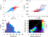 |
Fig. 3. Properties of UFs in a simulation with a chromospheric resonant cavity. Panel a: wavelength shift of the center of the emission core (Δv) as a function of the vertical velocity at log τ = −5.1 (vz). Panel b: maximum intensity of the emission feature as a function of the temperature fluctuation at log τ = −5.1. Panels a and b: blue dots represent upflowing UFs and red dots correspond to downflowing UFs. Panel c: histogram illustrating the duration of upflowing (blue bars) and downflowing (bars filled with red lines) UF events. Panel d: relation between the duration of the upflowing UFs and the preceding downflowing UFs. The color bar indicates the number of occurrences of UFs with the corresponding durations. |
Figure 3b shows the peak value of the emission core as a function of the temperature fluctuation. This fluctuation is defined as the difference between the actual temperature and that from the background model (at rest) at log τ = −5.1 (6100 K). Chromospheric temperature enhancements of at least 1000 K are required to produce a flashed profile. The intensity of the core shows small variations for temperature perturbations up to 1600 K. Higher temperature enhancements generate the strongest UFs found in the simulation, exhibiting a significant increase in the intensity of the core.
As previously pointed out, most of the flashes are associated with upflows, even in the case of standing oscillations. Panels c and d from Fig. 3 examine the duration of the upflowing and downflowing stages of UF events. We define the duration as the temporal span when the intensity core at a certain spatial location is continuously in emission (above the same previously defined threshold). Since upflowing UFs are generally preceded by downflowing UFs (Sect. 3.2), we measured the duration of each of these phases independently. Figure 3d shows that, in the vast majority of the cases, the upflowing stage lasts longer than the downflowing phase of the same event (the dashed white line marks the locations in the diagram where upflowing and downflowing UFs have the same duration). They are similar to the case illustrated in Fig. 2. For both downflowing and upflowing phases, the duration is generally in the range between 10 to 20 s, but the upflowing part of the UFs can extend longer than 25 s, whereas almost no downflows last that long. This explains the prevalence of detected UFs associated with upflows.
4. Discussion and conclusions
Umbral flashes are a well-known phenomenon, and their relation to the oscillatory processes in sunspot atmospheres is an established fact. Early modeling of UFs has characterized them as the result of upward-propagating waves (Havnes 1970; Bard & Carlsson 2010; Felipe et al. 2014). In this scenario, most of the line formation of UFs takes place at layers where the chromospheric flows generated by the oscillation are upflowing. The first spectropolarimetric analyses of UFs apparently confirmed this model (Socas-Navarro et al. 2000a; de la Cruz Rodríguez et al. 2013). However, recent studies have showed indications of a chromospheric resonant cavity above sunspot umbrae (Jess et al. 2020a), whose presence has been proved by Felipe et al. (2020) based on the analysis of the phase relations of chromospheric oscillations. Umbral chromospheric waves do not propagate but instead form standing waves.
In this study, we have modeled the development of UFs produced by standing oscillations for the first time. The phase shift between temperature and velocity fluctuations from standing waves differs from that of purely propagating waves. In the latter, temperature enhancements are associated with upflows, leading to upflowing UFs, whereas in standing oscillations the temperature increase takes place a quarter period earlier. This way, standing waves partially generate UFs during the downflowing stage of the oscillation. Interestingly, recent studies have started to report downflowing UFs (Henriques et al. 2017; Houston et al. 2020; Bose et al. 2019). Henriques et al. (2017) suggested that dowflowing UFs may be related to the presence of coronal loops rooted in sunspot umbrae since previous works have detected supersonic downflows in the transition region of such structures (e.g., Kleint et al. 2014; Kwak et al. 2016; Chitta et al. 2016). Our model offers an alternative explanation, interpreting downflowing UFs as a natural feature of the global process of sunspot oscillations. This is also the recent interpretation of Henriques et al. (2020), but here we show that such downflows are evidence of the standing-wave nature of these oscillations. Henriques et al. (2017) reported strong downflowing atmospheres for UFs, with velocities up to 10 km s−1, whereas our model produces downflowing UFs with velocities around 1 km s−1.
The development of UFs generated by standing waves is as follows. The chromospheric temperature starts to increase during the stage when the chromosphere is downflowing. All the chromospheric layers above the velocity resonant node are in phase and, thus, downflowing. This temperature increase is large enough to produce an emission core in the Ca II 8542 Å line. During the peak of the temperature fluctuation, the chromospheric plasma changes from downflowing to upflowing. The profiles remain flashed for the upflowing atmospheres until the chromospheric temperature again reaches a value closer to that of a quiescent umbra. Unfortunately, the temporal cadence of most Ca II 8542 Å observations to date, in the range between 25–28 s (e.g., Henriques et al. 2017; Joshi & de la Cruz Rodríguez 2018) and 48 s (Houston et al. 2020), is not sufficient to capture the evolution of UF events. The analysis is also challenged by the sudden variations in the atmosphere during the time required by Fabry-Perot spectrographs, such as the Interferometric BIdimensional Spectrometer (IBIS, Cavallini 2006) and the CRisp Imaging SpectroPolarimeter (CRISP, Scharmer et al. 2008), to scan the line (Felipe et al. 2018b). However, observations of small-scale umbral brightenings using a cadence of 14 s exhibit some indication of a temporal evolution consistent with that predicted by our modeling (Henriques et al. 2020). Upcoming observations with the National Science Foundation’s Daniel K. Inouye Solar Telescope (DKIST, Rimmele et al. 2020) will provide the ideal data for studying the temporal variations of UFs.
Our simulations show that the upflowing stage of UFs is generally longer than the downflowing part (Fig. 3d). This is in agreement with the prevalence of upflowing solutions in NLTE inversions of observed UFs (Socas-Navarro et al. 2000a; de la Cruz Rodríguez et al. 2013), even in studies where downflowing UFs are also reported (Houston et al. 2020).
This Letter provides a missing piece of the puzzle in what has been a convergence of observations and simulations: We have tied together the evidence for downflowing UFs and the existence of cavities in the chromosphere of the umbra as the latter will naturally generate the former. Finally, the case for a corrugated surface where downflows are significant (Henriques et al. 2020), together with the importance of cavities for such downflows, implies that future observations constraining the transition region of sunspots should find the transition region itself to be highly corrugated.
Acknowledgments
Financial support from the State Research Agency (AEI) of the Spanish Ministry of Science, Innovation and Universities (MCIU) and the European Regional Development Fund (FEDER) under grant with reference PGC2018-097611-A-I00 is gratefully acknowledged. VMJH is funded by the European Research Council (ERC) under the European Union’s Horizon 2020 research and innovation programme (SolarALMA, grant agreement No. 682462) and by the Research Council of Norway through its Centres of Excellence scheme (project 262622). JdlCR is supported by grants from the Swedish Research Council (2015-03994) and the Swedish National Space Agency (128/15). This project has received funding from the European Research Council (ERC) under the European Union’s Horizon 2020 research and innovation program (SUNMAG, grant agreement 759548). The authors wish to acknowledge the contribution of Teide High-Performance Computing facilities to the results of this research. TeideHPC facilities are provided by the Instituto Tecnológico y de Energías Renovables (ITER, SA). URL: http://teidehpc.iter.es.
References
- Al, N., Bendlin, C., & Kneer, F. 1998, A&A, 336, 743 [NASA ADS] [Google Scholar]
- Anan, T., Schad, T. A., Jaeggli, S. A., & Tarr, L. A. 2019, ApJ, 882, 161 [NASA ADS] [CrossRef] [Google Scholar]
- Avrett, E. H. 1981, in The Physics of Sunspots, eds. L. E. Cram, & J. H. Thomas, 235 [Google Scholar]
- Bard, S., & Carlsson, M. 2010, ApJ, 722, 888 [NASA ADS] [CrossRef] [Google Scholar]
- Beckers, J. M., & Tallant, P. E. 1969, Sol. Phys., 7, 351 [NASA ADS] [CrossRef] [MathSciNet] [Google Scholar]
- Berenger, J. P. 1994, J. Comput. Phys., 114, 185 [Google Scholar]
- Bharti, L., Hirzberger, J., & Solanki, S. K. 2013, A&A, 552, L1 [NASA ADS] [CrossRef] [EDP Sciences] [Google Scholar]
- Bose, S., Henriques, V. M. J., Rouppe van der Voort, L., & Pereira, T. M. D. 2019, A&A, 627, A46 [NASA ADS] [CrossRef] [EDP Sciences] [Google Scholar]
- Cavallini, F. 2006, Sol. Phys., 236, 415 [NASA ADS] [CrossRef] [Google Scholar]
- Centeno, R., Socas-Navarro, H., Collados, M., & Trujillo Bueno, J. 2005, ApJ, 635, 670 [NASA ADS] [CrossRef] [Google Scholar]
- Centeno, R., Collados, M., & Trujillo Bueno, J. 2006, ApJ, 640, 1153 [NASA ADS] [CrossRef] [PubMed] [Google Scholar]
- Chitta, L. P., Peter, H., & Young, P. R. 2016, A&A, 587, A20 [NASA ADS] [CrossRef] [EDP Sciences] [Google Scholar]
- Christensen-Dalsgaard, J., Dappen, W., Ajukov, S. V., et al. 1996, Science, 272, 1286 [CrossRef] [Google Scholar]
- de la Cruz Rodríguez, J., Rouppe van der Voort, L., Socas-Navarro, H., & van Noort, M. 2013, A&A, 556, A115 [NASA ADS] [CrossRef] [EDP Sciences] [Google Scholar]
- Deubner, F.-L. 1974, Sol. Phys., 39, 31 [NASA ADS] [CrossRef] [EDP Sciences] [Google Scholar]
- Felipe, T. 2019, A&A, 627, A169 [NASA ADS] [CrossRef] [EDP Sciences] [Google Scholar]
- Felipe, T. 2021, Nat. Astron., 5, 2 [NASA ADS] [CrossRef] [Google Scholar]
- Felipe, T., & Esteban Pozuelo, S. 2019, A&A, 632, A75 [NASA ADS] [CrossRef] [EDP Sciences] [Google Scholar]
- Felipe, T., Khomenko, E., Collados, M., & Beck, C. 2010a, ApJ, 722, 131 [NASA ADS] [CrossRef] [Google Scholar]
- Felipe, T., Khomenko, E., & Collados, M. 2010b, ApJ, 719, 357 [Google Scholar]
- Felipe, T., Khomenko, E., & Collados, M. 2011, ApJ, 735, 65 [NASA ADS] [CrossRef] [Google Scholar]
- Felipe, T., Socas-Navarro, H., & Khomenko, E. 2014, ApJ, 795, 9 [NASA ADS] [CrossRef] [Google Scholar]
- Felipe, T., Socas-Navarro, H., & Przybylski, D. 2018a, A&A, 614, A73 [NASA ADS] [CrossRef] [EDP Sciences] [Google Scholar]
- Felipe, T., Kuckein, C., & Thaler, I. 2018b, A&A, 617, A39 [NASA ADS] [CrossRef] [EDP Sciences] [Google Scholar]
- Felipe, T., Kuckein, C., González Manrique, S. J., Milic, I., & Sangeetha, C. R. 2020, ApJ, 900, L29 [Google Scholar]
- González-Morales, P. A., Khomenko, E., Downes, T. P., & de Vicente, A. 2018, A&A, 615, A67 [NASA ADS] [CrossRef] [EDP Sciences] [Google Scholar]
- Havnes, O. 1970, Sol. Phys., 13, 323 [NASA ADS] [CrossRef] [EDP Sciences] [Google Scholar]
- Henriques, V. M. J., & Kiselman, D. 2013, A&A, 557, A5 [NASA ADS] [CrossRef] [EDP Sciences] [Google Scholar]
- Henriques, V. M. J., Scullion, E., Mathioudakis, M., et al. 2015, A&A, 574, A131 [NASA ADS] [CrossRef] [EDP Sciences] [Google Scholar]
- Henriques, V. M. J., Mathioudakis, M., Socas-Navarro, H., & de la Cruz Rodríguez, J. 2017, ApJ, 845, 102 [NASA ADS] [CrossRef] [Google Scholar]
- Henriques, V. M. J., Nelson, C. J., Rouppe van der Voort, L. H. M., & Mathioudakis, M. 2020, A&A, 642, A215 [CrossRef] [EDP Sciences] [Google Scholar]
- Houston, S. J., Jess, D. B., Asensio Ramos, A., et al. 2018, ApJ, 860, 28 [NASA ADS] [CrossRef] [Google Scholar]
- Houston, S. J., Jess, D. B., Keppens, R., et al. 2020, ApJ, 892, 49 [NASA ADS] [CrossRef] [Google Scholar]
- Jess, D. B., Snow, B., Houston, S. J., et al. 2020a, Nat. Astron., 4, 220 [Google Scholar]
- Jess, D. B., Snow, B., Fleck, B., Stangalini, M., & Jafarzadeh, S. 2020b, Nat. Astron., 5, 5 [Google Scholar]
- Joshi, J., & de la Cruz Rodríguez, J. 2018, A&A, 619, A63 [NASA ADS] [CrossRef] [EDP Sciences] [Google Scholar]
- Khomenko, E., & Collados, M. 2006, ApJ, 653, 739 [Google Scholar]
- Kleint, L., Antolin, P., Tian, H., et al. 2014, ApJ, 789, L42 [NASA ADS] [CrossRef] [Google Scholar]
- Kwak, H., Chae, J., Song, D., et al. 2016, ApJ, 821, L30 [NASA ADS] [CrossRef] [Google Scholar]
- Maltby, P., Avrett, E. H., Carlsson, M., et al. 1986, ApJ, 306, 284 [Google Scholar]
- Nelson, C. J., Henriques, V. M. J., Mathioudakis, M., & Keenan, F. P. 2017, A&A, 605, A14 [NASA ADS] [CrossRef] [EDP Sciences] [Google Scholar]
- Rimmele, T. R., Warner, M., Keil, S. L., et al. 2020, Sol. Phys., 295, 172 [Google Scholar]
- Rouppe van der Voort, L., & de la Cruz Rodríguez, L., 2013, ApJ. 776, 56 [CrossRef] [Google Scholar]
- Scharmer, G. B., Narayan, G., Hillberg, T., et al. 2008, ApJ, 689, L69 [Google Scholar]
- Socas-Navarro, H., Trujillo Bueno, J., & Ruiz Cobo, B. 2000a, Science, 288, 1396 [NASA ADS] [CrossRef] [Google Scholar]
- Socas-Navarro, H., Trujillo Bueno, J., & Ruiz Cobo, B. 2000b, ApJ, 544, 1141 [NASA ADS] [CrossRef] [Google Scholar]
- Socas-Navarro, H., Trujillo Bueno, J., & Ruiz Cobo, B. 2001, ApJ, 550, 1102 [NASA ADS] [CrossRef] [Google Scholar]
- Socas-Navarro, H., McIntosh, S. W., Centeno, R., de Wijn, A. G., & Lites, B. W. 2009, ApJ, 696, 1683 [NASA ADS] [CrossRef] [Google Scholar]
- Socas-Navarro, H., de la Cruz Rodríguez, J., Asensio Ramos, A., Trujillo Bueno, J., & Ruiz Cobo, B. 2015, A&A, 577, A7 [NASA ADS] [CrossRef] [EDP Sciences] [Google Scholar]
- Wedemeyer-Böhm, S., & Carlsson, M. 2011, A&A, 528, A1 [NASA ADS] [CrossRef] [EDP Sciences] [Google Scholar]
- Wittmann, A. 1969, Sol. Phys., 7, 366 [NASA ADS] [CrossRef] [Google Scholar]
- Yurchyshyn, V., Abramenko, V., Kosovichev, A., & Goode, P. 2014, ApJ, 787, 58 [NASA ADS] [CrossRef] [Google Scholar]
- Zhugzhda, Y. D. 2008, Sol. Phys., 251, 501 [Google Scholar]
- Zhugzhda, Y. D., & Locans, V. 1981, Sov. Astron. Lett., 7, 25 [NASA ADS] [Google Scholar]
Appendix A: Numerical setup
The ideal magnetohydrodynamic (MHD) equations were solved using the code MANCHA (Khomenko & Collados 2006; Felipe et al. 2010b). The numerical simulations were computed using the 2.5D approximation. We employed a 2D domain, but vectors kept 3D coordinates. This code solves the nonlinear equations since UFs are characterized by acoustic shock waves. The shock-capturing capabilities of the code were validated by comparing its performance with analytic solutions of shock tube tests both in the MHD approximation (Felipe et al. 2010b) and including the effects of partial ionization (González-Morales et al. 2018). In this paper, we have restricted the analysis to ideal MHD. The vertical direction of the computational domain spans from z = −1140 km to z = 3500 km, with z = 0 set at the height where the optical depth at 5000 Å is unity (log τ = 0), and a constant spatial step of 10 km is used. At top and bottom boundaries, we imposed a perfectly matched layer (Berenger 1994), which damps waves with minimum reflection. The horizontal domain includes 96 points with a spatial step of 50 km. Periodic boundary conditions were imposed in the horizontal direction.
The code computes the temporal evolution of waves driven below the solar surface as they propagate in a background umbral model. The background atmosphere is constant in the horizontal direction. The vertical stratification of a modified (Avrett 1981) model was established at all horizontal locations. The modifications of this umbral atmosphere include the extension of the model to deeper layers by smoothly merging it with model S (Christensen-Dalsgaard et al. 1996) and the shift of the chromospheric temperature increase to higher layers. The latter was introduced to employ a model that generates Ca II 8542 Å profiles comparable to those observed in actual observations, similar to Felipe et al. (2018a). The model includes a sharp temperature gradient from chromospheric temperature values to coronal temperatures starting at z ≈ 1.8 Mm. The atmosphere is permeated by a vertical magnetic field with a constant strength of 2000 G. Waves are driven with a vertical force imposed at z = −180 km. The temporal and spatial dependences of the driver were extracted from temporal series measured in the photospheric Si I 10827 Å line (Felipe et al. 2018b) following the methods described in Felipe et al. (2011).
A total of 55 min of solar time were computed. The simulated atmospheres were saved with a temporal cadence of 5 s. For the analysis of the properties of UFs produced by standing waves (Sect. 3.3), we avoided the first 15 min of the simulation since during this time the first wavefronts are arriving in the chromosphere and the standing oscillations are not established. Thus, the analysis was restricted to the last 40 min of simulations.
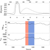 |
Fig. A.1. Response functions of the intensity profile of the Ca II 8542 Å line during the development of a UF. Panel a: response function of Stokes I to the temperature at the core of the line (dashed line) and to the velocity at the wavelength where the response is maximum (8542.2 Å, solid line) at t = 1405 s (see profile in Fig. 2k). The lower axis corresponds to the optical depth and the upper axis to the geometrical height. Panel b: optical depth of the maximum of the response function to temperature. Panel c: geometrical height of the maximum of the response function to temperature. The color-shaded regions in panels b and c have the same meaning as in Fig. 2. |
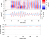 |
Fig. A.2. Numerical simulations of wave propagation in a sunspot umbra. Panel a: vertical velocity at z = 1.35 Mm for all the horizontal positions. Panel b: vertical velocity (red line, left axis) and temperature fluctuations (blue line, right axis) at X = −1.1 Mm (location indicated by the vertical green line in panel a). Panel c: average phase difference between velocity and temperature oscillations for waves with a frequency between 5 and 6 mHz as a function of atmospheric height. The red line represents the phase shift for standing waves from a simulation with a resonant cavity. The blue line corresponds to propagating waves from a simulation without a transition region. Dotted (dashed) lines indicate a phase shift of ±π/2 (0). |
Transition probabilities per second at log τ = −5 in the Maltby M sunspot model (Maltby et al. 1986).
Appendix B: Spectral synthesis
The Stokes profiles of the Ca II 8542 Å line were synthesized for all the spatial locations and time steps of the simulation using the NLTE code NICOLE (Socas-Navarro et al. 2015). NICOLE was fed with the velocity, temperature, gas pressure, density, and magnetic field vector stratification of each atmosphere (for a specific horizontal position and time) in a geometrical scale, as given by the output of the numerical simulation. An artificial macroturbulence of 1.8 km s−1 was added to compensate for the absence of small-scale motions in the numerical calculations and generate broader line profiles, similar to those measured in actual observations. The Stokes profiles were first synthesized with a spectral resolution of 5 mÅ. They were then degraded to a resolution of 55 mÅ by convolving them with a 100 mÅ full width half maximum Gaussian filter centered at the wavelengths chosen for the spectral sampling.
Table A.1 shows the transition probabilities from the lower level of the Ca II 8542 Å line to all other levels and vice versa. The large values point to very short characteristic transition times (below one second), confirming that the assumption of statistical equilibrium leads to very small decay times, shorter than the temporal scales of interest for our study. The only exceptions are the rates to and from the Ca II continuum (k = 6). The characteristic times for this transition are on the order of minutes, which means that ionization to Ca III might be lagging behind the dynamics. However, this is not relevant for our purposes since Ca II is the dominant species.
Figure A.1 illustrates the response function of the Ca II 8542 Å intensity to the temperature during the development of a UF. The main contribution to Stokes I comes from an optical depth around log τ = −5.1. We chose this optical depth as the reference for the analyses presented in this study since it is maintained as the main contribution to the formation of the line during the whole temporal span of UFs (color-shaded regions in Fig. A.1b). During this time, log τ = −5.1 samples a geometrical height around z = 1350 km (Fig. A.1c). Remarkable changes in the chromospheric region with higher sensitivity to the temperature are found between flashed and non-flashed profiles (ranging between log τ = −4.7 and log τ = −5.6).
Appendix C: Standing and propagating oscillations
Figure A.2 illustrates the chromospheric oscillations from the numerical simulation. Panel a shows the velocity wavefield for all the umbral spatial positions included in the simulation. We used the usual spectroscopic velocity convention in astrophysics where negative velocities correspond to upflows (blueshifts, indicated in blue in Fig. A.2a) and positive velocities represent downflows (redshifts, red in Fig. A.2a). Figure A.2b exhibits the temporal evolution of velocity (red line) and temperature (blue line) fluctuations at a randomly selected umbral location. Temperature wavefronts are delayed with respect to velocity wavefronts. For a better examination, Fig. A.2c shows the phase difference between temperature and velocity oscillations for waves with frequencies in the range 5–6 mHz (red line). Only the atmospheric heights of interest for the formation of the Ca II infrared lines are plotted. The phase shift is around π/2, indicating that temperature fluctuations lag velocity oscillations by a quarter period, in agreement with theoretical estimates of standing waves (Deubner 1974; Al et al. 1998).
The blue line in Fig. A.2c corresponds to the phase shift derived from a numerical simulation where the transition region is removed. Instead, a constant temperature atmosphere is set above z = 1.5 Mm (Felipe 2019; Felipe et al. 2020). In this situation, waves can freely propagate in the upper atmospheric layers and the phase relation between velocity and temperature fluctuations tends to π, the expected value for propagating waves. The phase shift from purely propagating waves (strictly π) is not obtained for two reasons. First, there are temperature gradients in the model (the temperature increase from the photospheric to the chromospheric temperature), which produce some partial wave reflections at z ≈ 1.6 Mm. Second, as waves propagate upward, they develop into shocks and temperature enhancements take place earlier, shifting toward the compression phase of the wave. To summarize, in the propagating-wave scenario (blue line in Fig. A.2c), temperature fluctuations are approximately in anti-phase with velocity oscillations, and temperature enhancements correspond to upflows. If a chromospheric resonant cavity is present (red line), temperature oscillations are shifted backward and their increase partially coincides with the downflowing stage of the oscillations. For waves with ≈5.5 mHz frequency, from z = 1.1 Mm to z = 1.8 Mm, the shift of temperature fluctuations is in the range between 25 and 80 s.
All Tables
Transition probabilities per second at log τ = −5 in the Maltby M sunspot model (Maltby et al. 1986).
All Figures
|
Fig. 1. Development of a UF produced by propagating waves as seen in Ca II 8542 Å. Panel a: temporal evolution of the vertical velocity (solid line, left axis), temperature (dashed black line, black right axis), and density (dashed red line, red right axis) fluctuations at z = 1.35 Mm. The blue shaded region corresponds to the time when a UF is identified in the Stokes profiles and the atmosphere is upflowing at log τ = −5.1. Lower panels: stokes I (left column), Stokes V (middle column), and atmospheric models (right column). Each row corresponds to a different time step, as indicated at the bottom of the first column panels and the vertical dotted lines in panel a. In the right column, the vertical velocity (solid line, left axis) and temperature (dashed line, right axis) of the atmospheric model is plotted. The vertical dashed line marks the height of log τ = −5.1. |
| In the text | |
|
Fig. 2. Same as Fig. 1, but for standing oscillations. The red shaded region in panel a indicates the time when a UF is identified in the Stokes profiles and the atmosphere is downflowing at log τ = −5.1. |
| In the text | |
|
Fig. 3. Properties of UFs in a simulation with a chromospheric resonant cavity. Panel a: wavelength shift of the center of the emission core (Δv) as a function of the vertical velocity at log τ = −5.1 (vz). Panel b: maximum intensity of the emission feature as a function of the temperature fluctuation at log τ = −5.1. Panels a and b: blue dots represent upflowing UFs and red dots correspond to downflowing UFs. Panel c: histogram illustrating the duration of upflowing (blue bars) and downflowing (bars filled with red lines) UF events. Panel d: relation between the duration of the upflowing UFs and the preceding downflowing UFs. The color bar indicates the number of occurrences of UFs with the corresponding durations. |
| In the text | |
|
Fig. A.1. Response functions of the intensity profile of the Ca II 8542 Å line during the development of a UF. Panel a: response function of Stokes I to the temperature at the core of the line (dashed line) and to the velocity at the wavelength where the response is maximum (8542.2 Å, solid line) at t = 1405 s (see profile in Fig. 2k). The lower axis corresponds to the optical depth and the upper axis to the geometrical height. Panel b: optical depth of the maximum of the response function to temperature. Panel c: geometrical height of the maximum of the response function to temperature. The color-shaded regions in panels b and c have the same meaning as in Fig. 2. |
| In the text | |
|
Fig. A.2. Numerical simulations of wave propagation in a sunspot umbra. Panel a: vertical velocity at z = 1.35 Mm for all the horizontal positions. Panel b: vertical velocity (red line, left axis) and temperature fluctuations (blue line, right axis) at X = −1.1 Mm (location indicated by the vertical green line in panel a). Panel c: average phase difference between velocity and temperature oscillations for waves with a frequency between 5 and 6 mHz as a function of atmospheric height. The red line represents the phase shift for standing waves from a simulation with a resonant cavity. The blue line corresponds to propagating waves from a simulation without a transition region. Dotted (dashed) lines indicate a phase shift of ±π/2 (0). |
| In the text | |
Current usage metrics show cumulative count of Article Views (full-text article views including HTML views, PDF and ePub downloads, according to the available data) and Abstracts Views on Vision4Press platform.
Data correspond to usage on the plateform after 2015. The current usage metrics is available 48-96 hours after online publication and is updated daily on week days.
Initial download of the metrics may take a while.