| Issue |
A&A
Volume 693, January 2025
|
|
|---|---|---|
| Article Number | A165 | |
| Number of page(s) | 11 | |
| Section | The Sun and the Heliosphere | |
| DOI | https://doi.org/10.1051/0004-6361/202452317 | |
| Published online | 14 January 2025 | |
Observations of umbral flashes in the resonant sunspot chromosphere
1
Instituto de Astrofísica de Canarias, 38205 C/ Vía Láctea, s/n, La Laguna, Tenerife, Spain
2
Departamento de Astrofísica, Universidad de La Laguna, 38205 La Laguna, Tenerife, Spain
3
Institut für Sonnenphysik (KIS), Georges-Köhler-Allee 401a, 79110 Freiburg, Germany
⋆ Corresponding author; This email address is being protected from spambots. You need JavaScript enabled to view it.
Received:
20
September
2024
Accepted:
24
November
2024
Abstract
Context. In sunspot umbrae, the core of some chromospheric lines exhibits periodic brightness enhancements known as umbral flashes. The consensus is that they are produced by the upward propagation of shock waves. This view has recently been challenged by the detection of downflowing umbral flashes and the confirmation of a resonant cavity above sunspots.
Aims. We aim to determine the propagating or standing nature of the waves in the low umbral chromosphere and confirm or refute the existence of downflowing umbral flashes.
Methods. Spectroscopic temporal series of Ca II 8542 Å, Ca II H, and Hα in a sunspot were acquired with the Swedish Solar Telescope. The Hα velocity was inferred using bisectors. Simultaneous inversions of the Ca II 8542 Å line and the Ca II H core were performed using the code NICOLE. The nature of the oscillations were determined and insights into the resonant oscillatory pattern were gained by analyzing the phase shift between the velocity signals and examining the temporal evolution.
Results. Propagating waves in the low chromosphere are more common in regions with frequent umbral flashes, where the transition region is shifted upward, making resonant cavity signatures less noticeable. In contrast, areas with fewer umbral flashes show velocity fluctuations that align with standing oscillations. Evidence suggests dynamic changes in the location of velocity-resonant nodes due to variations in the transition region height. Downflowing profiles appear at the onset of some umbral flashes, but upflowing motion dominates during most of the flash. These downflowing flashes are more common in standing umbral flashes.
Conclusions. We confirm the existence of a chromospheric resonant cavity above sunspot umbrae. It is produced by wave reflections at the transition region. The oscillatory pattern depends on the transition region height, which exhibits spatial and temporal variations due to the impact of the waves.
Key words: Sun: atmosphere / Sun: chromosphere / Sun: oscillations / sunspots
© The Authors 2025
 Open Access article, published by EDP Sciences, under the terms of the Creative Commons Attribution License (https://creativecommons.org/licenses/by/4.0), which permits unrestricted use, distribution, and reproduction in any medium, provided the original work is properly cited.
This article is published in open access under the Subscribe to Open model. This email address is being protected from spambots. You need JavaScript enabled to view it. to support open access publication.
1. Introduction
Umbral flashes are sudden brightenings that appear in the core of some chromospheric lines in sunspot umbrae. Since their first detection in the late 1960s (Beckers & Tallant 1969; Wittmann 1969), they were interpreted as the result of waves propagating from the photosphere to the upper chromospheric layers. Their amplitude increases due to the drop of the density (e.g., Centeno et al. 2006), leading to shocks that heat the umbral chromosphere and produce a reversal in the line core, which appears in emission during the umbral flash event (Havnes 1970).
Earlier studies of umbral flashes based on the analysis of spectropolarimetric observations revealed velocity fluctuations that agree with the scenario of an upward wave propagation. Using nonlocal thermodynamic equilibrirum (NLTE) inversions, Socas-Navarro et al. (2001) modeled umbral flashes as two atmospheric models inside the resolution element, including one hot upflowing component. Subsequent spectropolarimetric inversions from observations with higher spatial resolution also found that umbral flashes occur when the atmosphere exhibits strong upflows (de la Cruz Rodríguez et al. 2013). This association of upflows with intensity (temperature) enhancements agrees with the accepted consensus that umbral flashes are a sign of upward-propagating waves. Numerical modeling of sunspot oscillations, including the synthesis of the spectral line profiles, also supports the mechanism of propagating waves as the cause of upflowing umbral flashes (Bard & Carlsson 2010; Felipe et al. 2014, 2018).
However, recent NLTE inversions have identified umbral flash profiles that were better fit by atmospheric models with strong downflows (Henriques et al. 2017; Bose et al. 2019; Houston et al. 2020). The inversions by Henriques et al. (2017) found that 60% of the umbral flashes correspond to atmospheres with downflows stronger than 3 km s−1. These results challenge the widely accepted view of umbral flashes. Felipe et al. (2021a) proposed that downflowing umbral flashes can appear as a result of standing oscillations in the sunspot chromosphere. In this model, temperature enhancements produced by the standing wave partially coincide with the downflowing stage of the oscillation, and the core of the Ca II 8542 Å can appear in emission when the atmosphere is downflowing. The chromospheric temperature continues to increase, while the atmosphere suddenly changes from downflowing to upflowing. In this way, the atmosphere exhibits upflowing velocities during most of the umbral flash event. This model is based on the presence of a resonant cavity in sunspot chromospheres that is produced by waves that are trapped between the temperature gradients of the transition region and the photosphere (Zhugzhda & Locans 1981; Zhugzhda 2008). The existence of this cavity above sunspot umbrae was recently confirmed (see Jess et al. 2020, 2021; Felipe et al. 2020; Felipe 2021).
We present a thorough analysis of the intensity profiles of chromospheric lines in a sunspot umbra. We focus on the velocity inferences and velocity oscillatory phase to provide unique insights into the nature of umbral waves and the origin of umbral flashes. The organization of the paper is as follows: In Sect. 2 we present the observed data, Sect. 3 describes the methods we employed for the analysis of the observations, and Sect. 4 shows the results, which are further discussed in Sect. 5. Finally, the main conclusions are summarized in Sect. 6.
2. Observations
The target of the observations was the sunspot from active region NOAA 13001. The data were acquired on 2022 May 3, when the sunspot was located at solar coordinates (x = 93″, y = −457″), with the Swedish 1 m Solar Telescope (SST; Scharmer et al. 2003). Simultaneous multiline observations in the Ca II 8542 Å, Ca II H, Hα, and Hβ lines were taken using the CRisp Imaging SpectroPolarimeter (CRISP; Scharmer 2006; Scharmer et al. 2008) and CHROMospheric Imaging Spectrometer (Scharmer 2017). We study a temporal series of spectroscopic data acquired between 09:36 and 10:16 UT. The analysis is complemented by ten full spectropolarimetric maps of the Ca II 8542 Å line that were acquired immediately before the spectroscopic series, between 09:29 and 09:35 UT.
The CRISP instrument was employed to scan the Ca II 8542 Å and Hα lines. The spatial sampling was  . The diffraction limit of the SST (computed as λ/D, where λ is the wavelength of the observed line, and D = 0.97 m is the diameter of the telescope) is
  for Ca II 8542 Å and
  for Hα. The Ca II 8542 Å was sampled with a total of 25 wavelength points. Around the core of the line (between −390 and +390 mÅ), the step was δλ = 65 mÅ, and a coarser resolution of 2δλ was used in the wings up to ±1040 mÅ. Two additional points were scanned at ±1755 mÅ. The Hα line was sampled at 21 wavelength positions, with steps of 100 mÅ between −800 and +800 mÅ for the line center and a twice coarser resolution between ±800 and ±1200 mÅ. The temporal cadence of the CRISP spectroscopic series was 12.30 s.
The Ca II H and Hβ data were acquired with CHROMIS. It has a spatial sampling of  and a diffraction limit of
  and
and  at the wavelengths of the Ca II H and Hβ lines, respectively. The Ca II H line was sampled from −455 to +455 mÅ in steps of 65 mÅ, between ±455 and ±845 mÅ in steps of 130 mÅ, and between ±845 and ±1235 mÅ in steps of 195 mÅ. An additional scan at a wavelength of 4000 Å was also acquired for a total of 26 points. The Hβ line was scanned with the same wavelength sampling as was used for Hα. The temporal cadence of the CHROMIS spectroscopic series was 12.37 s.
The data were processed using the pipeline SSTRED (Löfdahl et al. 2021), which employs multi-object multi-frame blind deconvolution (MOMFBD; van Noort et al. 2005; Löfdahl 2002). It implements the methods to produce science-ready data from the CRISP and CHROMIS raw observations. The pipeline for the former instrument was previously described in de la Cruz Rodríguez et al. (2015).
3. Data analysis
3.1. Identification of umbral flash profiles
We focused on the study of umbral fluctuations. The umbral region was selected by applying an intensity threshold in the Ca II 8542 Å maps at Δλ = 1755 mÅ. Within the umbra, we labeled as umbral flashes those profiles in which the maximum intensity between Δλ = −325 mÅ and Δλ = 0 mÅ was higher than the intensity at Δλ = 650 mÅ. The bottom panels of Fig. 1 illustrate the location of the umbral flashes during the temporal period analyzed in this work (last 13 min of the spectroscopic temporal series).
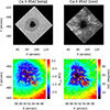 |
Fig. 1. Field of view of the observations and magnetic field inferred from the inversions of the polarimetric map. Top panels: intensity in the wing (left panel) and core (right panel) of the Ca II 8542 Å line. The white square delimits the region in which the spectropolarimetric inversions were performed. Bottom panels: line-of-sight magnetic field (left panel) and magnetic field inclination (right panel). The white contours mark the boundary between the umbra and penumbra. The red, orange, and yellow contours delimit the regions in which 14, 7, and 3 umbral flash profiles, respectively, were detected during the 13 min of the temporal series that we analyzed. |
3.2. Spectropolarimetric inversions
Full spectropolarimetric inversions of a Ca II 8542 Å map were performed using the NLTE inversion code NICOLE (Socas-Navarro et al. 2015). In the presence of magnetic fields, the code calculates the polarization resulting from Zeeman splitting. The Ca II atom model we employed encompasses five bound levels and a continuum (de la Cruz Rodríguez et al. 2012). Collision-induced line broadening was evaluated using the approach described by Anstee & O’Mara (1995).
We constructed a sunspot map free of umbral flash profiles as follows. From the series of ten spectropolarimetric maps, we chose the map that was acquired under better seeing conditions (as indicated by the Fried parameter r0) and replaced the profiles in which the core of the Ca II 8542 Å line was in emission by profiles from the same locations, scanned 69 s later. This approach provided us with a map of the quiescent umbra in which no locations were impacted by the striking changes produced by umbral flashes.
The inversions of the polarimetric map were restricted to the sunspot umbra and surroundings. They were performed using three cycles. The last cycle included ten nodes for temperature, six nodes for velocity, two nodes for microturbulence and longitudinal magnetic field, and one node for the transversal components of the magnetic field. Figure 1 illustrates the whole field of view of the observations in Ca II 8542 Å and the inversion results for the chromospheric magnetic field along the line of sight (LOS) and inclination. A median filter, replacing the value of each element by the median found in a 5 × 5 window around the element, was applied to the two inverted maps. The discrepancy between the umbra intensity contours and the LOS magnetic field strength arises from the position of the sunspot on the solar disk. Near the northern umbral boundary, the inclined magnetic field lines (concerning the local reference frame) are more aligned with the LOS, and thus, a stronger LOS magnetic field is measured there.
3.3. Multiline spectroscopic inversions and degeneracy of the solutions
Simultaneous inversions of the Ca II 8542 Å and Ca II H lines were performed using NICOLE. The code NICOLE operates under the assumption of a full angle and frequency redistribution, along with a plane-parallel atmosphere for every pixel. This is a suitable approximation for the Ca II 8542 Å since it is weakly affected by partial redistribution effects (Uitenbroek 1989). In contrast, the Ca II H and Ca II K lines are formed at higher chromospheric layers, in which partial redistribution is more important (Vardavas & Cram 1974; Uitenbroek 1989; Solanki et al. 1991; Bjørgen et al. 2018). These effects are especially fundamental in the wings of the lines. Previous works have independently modeled the core and the wings of some of these lines, including 3D radiative transfer and complete redistribution in the core and 1.5D radiative transfer and partial redistribution in the wings (Pereira et al. 2013). We restricted the multiline inversions to the core of the Ca II H line and to the full Ca II 8542 Å profile, where the impact of partial redistribution effects is weaker. Only the wavelengths of the Ca II H line between Δλ = −130 mÅ and Δλ = 65 mÅ (four spectral points) were used for the inversions. A weight twice higher than the weight of the Ca II 8542 Å was assigned to these points.
The Ca II 8542 Å and Ca II H profiles were acquired with different instruments that had a different spatial sampling and temporal cadence. For the inversions, we selected a Ca II 8542 Å profile (from the CRISP instrument because its spatial sampling is coarser) and searched for the Ca II H profile, whose spatial location and time is closer to the chosen Ca II 8542 Å spectrum. This means that the profiles of the two lines are not strictly cospatial and cotemporal. In the following analyses, we focused on 44 spatial locations to sample the sunspot umbra. These locations (illustrated by colored circles in Fig. 2) were selected at positions in which the distance between CRISP and CHROMIS pixels was smaller than 0″01. The maximum time shift between the profiles of the two instruments is around 6 s. We focused the analysis on the cases when the two lines were acquired nearly simultaneously, and we allowed a maximum time difference of roughly 2.5 s. The temporal cadence of the two instruments is similar (12.30 and 12.37 s for CRISP and CHROMIS, respectively), and the temporal coherence was therefore reasonably maintained for successive scans. Following this criterion, we focused the analysis on the last 13 min of the spectroscopic series.
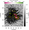 |
Fig. 2. V-V phase shift between the Ca II and Hα chromospheric velocities at the analyzed locations. The background shows an intensity map of the umbra and surroundings at the continuum around the Ca II 8542 Å line. The colored dots mark the analyzed locations, and the color corresponds to the V-V phase shift at 6.45 mHz according to the upper color bar. The contours indicate the number of umbral flash profiles as described in Fig. 1. The letters A-D indicate the locations illustrated in Figs. 6, 8, 9, and 10. |
In order to minimize the uncertainty of the results of the NLTE inversions due to the degeneracy of the solutions (e.g., Felipe et al. 2021b), we performed a total of 256 inversions from each analyzed profile. They differed in the initial guess atmosphere, the number of employed nodes, and the regularization parameter. Every independent inversion was carried out using a scheme of several cycles with increasing complexity in the node distribution. The number of nodes for the last cycle varied between six and ten for the temperature, two and six for the velocity, and one and two for the microturbulence. In the inversions of the spectroscopic temporal series, the magnetic field was not inverted. Instead, the value of the magnetic field vector extracted from the inversion of the spectropolarimetric map (Sect. 3.2) at the corresponding location was imposed. NICOLE inversions generally include regularization. This is a free parameter that can be set to values between zero and one. Values near one tend to favor vertically smooth profiles, whereas regularization near zero will allow solution atmospheres with strong vertical variations. In the set of control files we used for the inversions, the regularization ranged from 0.1 to 1. The process was parallelized using the parallel command (Tange 2018).
From the total of 256 independent inversions performed for each profile, we chose a set of best inversions. This selection was based on the χ2 value, which characterizes the difference between the synthetic profiles generated by the atmosphere obtained from the inversion and the actual observed atmosphere. Since a lower χ2 value indicates a better agreement, we imposed a maximum value in χ2. When fewer than five inversions satisfied this threshold in χ2, we selected the five inversions with lower χ2 instead. The value of χ2 computed by NICOLE depends on the weights of the wavelengths and on the regularization parameter. To illustrate the quality of the inversion fits, we plot an example umbral flash profile (top panels in Fig. 3). This example corresponds to a situation in which only one of the inversions is below the threshold, so that four out of the five selected inversions have a χ2 above that value (bottom panel in Fig. 3). The blue lines in the top panels show the synthetic profiles obtained from the inversion whose χ2 value is just below the chosen threshold, whereas the red lines indicate the profiles for the highest χ2 inversion from the five selected cases. The comparison shows that even when only a few inversions meet our threshold criterion, the fits are still sufficiently good. In general, during umbral flash events, the inversions are more challenging, and we restricted the analysis to a set of 5 to 20 inversions. For quiescent profiles, many inversions (up to ∼200) satisfy the threshold criterion.
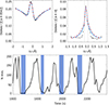 |
Fig. 3. Quality of the inversion fits and number of inversions that satisfy the threshold criterion. Top panels: observed umbral flash profile (black dots), the fit obtained from an inversion whose χ2 is near the chosen threshold (solid blue line), and the fit of the inversion with the worst χ2 (above the threshold) that was included in the analysis (dashed red line). The left panel corresponds to the Ca II 8542 Å line, and the right panel shows the Ca II H line. The vertical dotted lines in the right panel delimit the line core region we employed in the inversions. Bottom panel: temporal evolution of the number of inversions employed for the analysis of each profile at a selected umbral location. The blue shaded areas indicate the temporal steps when the core of the Ca II 8542 Å is in emission. The vertical dotted line corresponds to the time step illustrated in the top panels. |
Figure 4 illustrates the degeneracy of the solutions and the necessity of including the core of the Ca II H line in the inversions. It represents the results from the inversions at an umbral location, with the focus on the profiles from one temporal step with strong differences between the multiline and single-line inversions. The same approach was followed for both cases, and the only difference was that in the single-line inversions, the weights of the Ca II H line core were set to zero. The chromospheric velocity (averaged between log τ = −4.6 and log τ = −5.3) of the single-line inversions agrees well with that obtained from the multiline inversions in most of the temporal series, except around the end of the umbral flash events. At these times, the single-line inversion (violet line) shows a sudden change from negative (upflowing) to positive (downflowing) velocity. In contrast, the multiline inversion exhibits a progressive change in the velocity from upflows toward downflows, as expected from the temporal evolution of chromospheric velocity fluctuations in sunspot umbrae (e.g., Centeno et al. 2006). The bottom panels illustrate the inversions for one of the cases in which this discrepancy is obvious. The stratification of the velocity in the single-line inversion exhibits two independent branches, one with remarkably high negative velocities, and the other with strong positive velocities. The median velocity (solid violet line) tracks the latter branch of the solutions since most of them are gathered there. The addition of the core of the Ca II H line to the inversions breaks this degeneracy, and solutions with positive (downflowing) velocity are discarded. It also benefits temperature estimations. During the whole temporal series, the standard deviation of the multiline inversion temperature is significantly lower than that of the single-line inversions (second panel from Fig. 4). This is also shown in the temperature stratification (bottom panels from Fig. 4), where the dispersion of the solutions in the chromosphere is much larger when only the Ca II 8542 Å line is inverted.
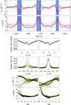 |
Fig. 4. Comparison of single-line inversions of the Ca II 8542 Å and multiline inversions of that line together with the core of the Ca II H at a randomly chosen umbral location. Top panel: temporal evolution of the chromospheric velocity inferred from multiline (red line) and single-line (violet) inversions. The velocity value is given by the median of the set of best inversions from the 256 independent inversions performed for each spectral profile. The error indicates the standard deviation of that set. Second panel: same as the top panel, but for the temperature. In the top two panels, the blue shaded areas indicate the times when the Ca II 8542 Å profile exhibits an umbral flash. The vertical dotted line at t = 1697 s marks the time illustrated in the bottom panels. Four bottom rows: inversion results for the single-line (left column) and multiline (right column) inversions. The top two rows illustrate the observed line profiles (red dots) and the fit of the inversions. The bottom two rows correspond to the stratification of the velocity and temperature inferred from the inversions. In all these panels, the green color scale indicates how common a solution is in the set of best inversions (a darker color corresponds to a more common solution). In the bottom two rows, the solid lines illustrate the median solution from the set of best inversions, and the dotted lines indicate the standard deviation. |
3.4. Hα velocity
The line-of-sight velocity of the Hα profiles was estimated using bisectors (Kulander & Jefferies 1966; González Manrique et al. 2020). This technique provides height-dependent velocity information by measuring the shift between the static line center and the line bisector. The measurement of the bisectors at different intensity levels, from the core to the wings of the line, gives the velocity at different atmospheric layers.
We derived the Hα velocity for all the sunspot locations and the full temporal series using several bisectors, with intensities at 5%, 10%, 20%, 30%, 40%, and 50% of the line, where 0% corresponds to the line core and 100% corresponds to the outer wings. The velocity computed with bisectors closer to the continuum level (beyond 60%) produced noisy velocity maps that were discarded. In the following, we focus on the analysis of the 10% bisectors. The other percentage line depths were also evaluated, but we found no significant differences with the 10% case.
3.5. V-V phase shift
The multiline spectroscopic inversions described in Sect. 3.3 were performed for 63 time steps (around 13 min) at 44 spatial positions. The locations were selected to sample sunspot regions with different umbral flash activities. The chosen locations are marked in Fig. 2 by colored dots. Several locations were selected in the umbral region in which flashed profiles are prevalent (more than 13 profiles during the analyzed period; red contour in Fig. 2), some in the region with a moderate frequency of umbral flashes (between 7 and 12 flashed profiles; orange contours) and with a low frequency of flashes (between 3 and 6 profiles; yellow contours). For completeness, we also included two locations without umbral flashes.
The color of the dots indicates the V-V phase difference between the chromospheric velocity inferred from the multiline inversion of the Ca II lines and the Hα velocity (ΔϕVV[Ca II 8542–Hα]) at the frequency at which the power of the chromospheric velocity oscillations is highest (6.45 mHz). The phases were directly computed from the Fourier transform of the velocity signals at the same spatial location. A phase shift of ΔϕVV[Ca II 8542–Hα] = 0 rad (dark pink) indicates that both velocity signals are in phase, whereas ΔϕVV[Ca II 8542–Hα] = π rad (dark green) corresponds to oscillations in opposite phase. A positive phase difference indicates a delay of the Hα velocity signal with respect to the Ca II chromospheric velocity.
Based on the height difference between the chromosphere probed by the inversions of the Ca II lines and the formation height of Hα (around 265 km; see Sect. 4.1) and the position of the sunspot on the solar disk, we expect a displacement of more than two pixels (from the CRISP instrument) across the plane of sky between both signals. We did not take this displacement into account when we computed the V-V phase shift between the velocity signals from these two atmospheric layers. However, we argue that this issue does not compromise the results from the phase difference analysis. We computed the phase difference between the Hα velocity in each selected location (44 cases) and all the surrounding positions within a diameter of four pixels. The results are shown in Fig. 5 as a function of the magnetic field inclination. In all cases, the average phase difference is around zero and the standard deviation is low, indicating that Hα velocity oscillations are coherent over spatial scales larger than the projection shift on the plane of the sky. The phase difference results between the Ca II 8542 Å and Hα velocities are not significantly impacted by the fine determination of the Hα location. The situation is more complex when the propagation of slow magnetoacoustic waves (e.g., those studied in this work) along the magnetic field lines is taken into account. Depending on the orientation of the magnetic field, they could balance the projection displacement or increase it. However, the results from Fig. 5 do not depend on the inclination, which proves that the measured dispersion in the Hα velocity phase of neighboring points is not due to the propagation of the waves along the magnetic field lines.
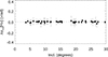 |
Fig. 5. Average phase difference between the velocity measured in Hα at the locations analyzed in this study and the surrounding pixels within a diameter of four pixels. The results are plotted as a function of the local magnetic field inclination. The error bars indicate the standard deviation. |
4. Standing or propagating nature of chromospheric umbral waves
The phase shift between the chromospheric velocity inferred from the inversion of the Ca II lines and the Hα velocity was used to determine the standing or propagating character of the waves at each analyzed location. Standing waves oscillate in time, but the peak amplitude of the wave does not move in space. Instead, they form a stationary wave pattern, with specific points of minimum amplitude (nodes) and maximum amplitude (antinodes). The locations in the same region of the wave pattern (e.g., between two nodes) oscillate in phase, whereas two points with an odd number of nodes between them oscillate in antiphase. Propagating waves move in space. For example, the wavefronts in the lower solar atmosphere progressively move upward. Each point throughout the wave has a different phase, as opposed to standing oscillations, and the measurement of the phase difference between the fluctuations at two layers can be used to track and characterize this wave propagation.
The phase shifts between the chromospheric velocity signals illustrated in Fig. 2 exhibit various values depending on the location. This indicates the inhomogeneous nature of the chromospheric waves at the layers probed by the Ca II lines and Hα. Moreover, the highly dynamic umbral chromosphere, with the umbral flashes as its main feature, produces shifts in the transition region and formation height of the lines. In this way, the oscillations can exhibit different behaviors in a fixed location. In the following subsections, we illustrate these insights by showing the results at some selected locations.
4.1. Propagating waves in regions with a high frequency of umbral flashes
Figure 6 shows the temporal evolution of the velocity and temperature chromospheric fluctuations in location A, indicated in Fig. 2. In the following, the discussion of the inverted velocity and temperature signals refers to the averages in the optical depth range between log τ = −4.6 and log τ = −5.3. Location A corresponds to a selected location within the region in which umbral flash profiles are most common (more than 13 flash profiles in the analyzed series). In this region, the phase shift between the two velocity signals is around 0.4π (shown in light pink in Fig. 2). This phase difference corresponds to a delay of around 31 s in the Hα velocity signal with respect to the Ca II chromospheric velocity, as shown in the top panel of Fig. 6. Since the wavefronts require more time to reach the higher formation heights of the Hα line, this result is consistent with the presence of upward-propagating waves between the layers probed by the Ca II lines and Hα. When we assume that waves are free to propagate vertically at the chromospheric sound speed (around 8.5 km s−1, Maltby et al. 1986) in all locations between these two layers, this delay corresponds to a height difference of roughly 265 km between the response height of the two velocity signals.
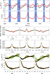 |
Fig. 6. Temporal evolution of the chromospheric fluctuations and inversion results at point A from Fig. 2, where propagating waves are found in the low chromosphere. Top panel: chromospheric velocity inferred from the multiline inversions of the Ca II lines (red line) and from Hα (black line). The inverted velocity corresponds to the median of the set of best inversions (out of 256 independent inversions) averaged in the optical depths between log τ = −4.6 and log τ = −5.3. The error bars indicate the standard deviation of the set of best inversions. Second panel: chromospheric temperature inferred from the inversion of the Ca II lines. The median temperature and error bars were determined similarly to the velocity. Middle panels: intensity of the Ca II 8542 Å (third row) and the Ca II H (fourth row) lines at three time steps indicated by vertical dashed lines in the top two panels. Bottom panels: inversion results for the velocity (fifth row) and temperature (last row) for the three selected time steps. The green color scale has the same meaning as in Fig. 4. |
The region with a high number of umbral flash profiles (locations in which we identified more than 13 flashed profiles; red contour in Fig. 2) was sampled in 14 locations. During the 13 min of the temporal series we analyzed, five independent umbral flash events took place in every location, as shown in the top panels of Fig. 6. The duration of umbral flash events is variable. The longest cases exhibit flash profiles in Ca II 8542 Å during five consecutive time steps (61.5 s). Almost all umbral flashes are associated with negative velocities (upflows), except for a few exceptions. Figure 7 illustrates one of these exceptions. The Ca II 8542 Å core is in emission for three consecutive time steps (36.9 s). At the first step, the chromospheric velocity inferred from the inversion of the Ca II lines exhibits a strong downflow. As the umbral flash event evolves, the Ca II velocity sharply changes from positive to negative (downflow to upflow) as the core emission is enhanced.
4.2. Umbral flashes produced by standing waves: Velocity fluctuations in phase
The phase shifts illustrated in Fig. 2 show a clear difference between the locations in the region with a high number of umbral flashes (red contour) and the surroundings. The analyzed positions located slightly further north exhibit a phase shift around zero, which indicates that the Ca II and Hα velocity fluctuations are in phase. When we take the height difference between the probed velocity signals into account (as seen in the previous section), this indicates that oscillations in these locations are mostly produced by standing waves.
Figure 8 shows the results at the position marked B in Fig. 2, which is one of the locations in which we detected standing waves. During most of the temporal series, especially between t ∼ 1660 s and t ∼ 2100 s, both velocity signals fluctuate in phase. The figure shows the spectral profiles and inversions during the first umbral flash event in the analyzed temporal series. In this case, the umbral flash begins when the chromospheric layer probed by the Ca II lines is downflowing, and it continues with a sudden change to upflows, similar to the propagating case illustrated in Fig. 7. Although the majority of umbral flash events are associated with upflowing chromospheres at all time steps with a Ca II 8542 Å emission core, in the case of standing oscillations the evolution from downflowing to upflowing during the flash is more common. Out of the 57 independent umbral flash events produced by standing oscillations that we sampled, 13 exhibit a downflowing chromosphere at the initial flashed profile. For the propagating waves we explored in the previous subsection, only 3 out of 64 events show this behavior.
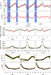 |
Fig. 8. Same as Fig. 6, but for point B in Fig. 2, where standing waves are found in the low chromosphere. |
4.3. Umbral flashes produced by standing waves: Velocity fluctuations in antiphase
In the region around [x = 89″, y = −455″], we found a moderate number of umbral flash profiles for which the phase difference between the two chromospheric velocity signals is around π, that is, the chromospheric velocity fluctuations in the Ca II lines and Hα are approximately in opposite phase. We also identified velocity fluctuations in antiphase in the two sampled locations in regions that are free of umbral flash profiles, corresponding to the darker part of the umbra, where the magnetic field is stronger.
Figure 9 illustrates the results in an interesting location in this region (location C in Fig. 2). Even though the velocity inferred from the inversions exhibits some dispersion, the solutions converge at the chromospheric height used for the velocity signal illustrated in the top panel (log τ between −4.6 and −5.3). The velocity fluctuations are in phase at some times, for example, after t = 2100 s and at the initial times (between t = 1600 and t = 1750 s). This is consistent with the results presented in the previous subsection, where velocity fluctuations in phase at different low chromospheric layers indicated that oscillations are mostly produced by standing waves.
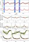 |
Fig. 9. Same as Fig. 6, but for point C in Fig. 2, where standing waves are found in the low chromosphere. |
In contrast, between t ∼ 1800 and t ∼ 2000 s (approximately for one and a half period), the two velocity signals fluctuate with opposite phases. This result is also consistent with the presence of standing oscillations. We expect to find this behavior when the heights of the chromospheric velocities probed with the inversions of the Ca II lines and with Hα are at different sides of a velocity-resonant node. The height of the inferred velocities with respect to the resonant node results from an interplay between changes in the formation height of the lines and dynamic variations in the height of the transition region. We identified different behaviors in the V-V phase shifts between the Hα y Ca II velocities (propagating waves, standing waves in phase, and standing waves in opposite phase), even though the chromospheric inferences (velocity and temperature evolutions) are similar. In this way, we consider that the main driver of the changes in the oscillatory pattern is the height of the transition region.
Our results show that the transition region height is not only inhomogeneous in the umbra, but also highly dynamic. A fixed spatial location can exhibit remarkable changes in the height of the reflecting layer that produces the resonant cavity, and thus, the height of the resonant nodes.
4.4. Umbral flashes produced by standing waves: Ca II 8542 Å core reversal with vanishing velocity
Figure 10 presents another example of a location (location D in Fig. 2) in which the velocity signals are predominantly in antiphase. This observation is consistent with standing oscillations, indicating that the probed heights are on opposite sides of a velocity node. Interestingly, between t = 1900 and t = 2030 s, the Hα velocity exhibits remarkable velocity fluctuations with a peak-to-peak amplitude of approximately 9 km s−1. In contrast, the Ca II velocity signal is absent, showing a velocity around zero for nearly an entire oscillatory period. However, during this time, the temperature fluctuations display a pronounced peak.
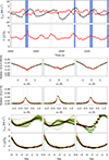 |
Fig. 10. Same as Fig. 6, but for point D in Fig. 2, where standing waves are found in the low chromosphere. |
The oscillatory behavior observed during this temporal period also supports the presence of standing oscillations. At the height of the velocity nodes, the velocity fluctuations have zero amplitude. In this example, the chromospheric height probed by the inversions of the Ca II lines corresponds for some time to the height of a velocity node. The Hα line, formed a few hundred kilometers above and away from the velocity node, does exhibit significant velocity fluctuations. We emphasize that the height difference between the response of the two velocity signals is not sufficient to explain the large difference in the amplitude of the observed velocity if it were produced by the drop in the density between the two layers. The presence of a velocity node at the formation height of the Ca II lines is the only scenario that can account for these observations.
We also stress that in the chromospheric resonant cavity, the height of the velocity-resonant nodes differs from that of the temperature resonant nodes (see, e.g., Fig. 3 from Fleck & Deubner 1989). Even when we assume that the velocity and temperature signals obtained from the inversion of the Ca II lines probe similar atmospheric layers, this region does not correspond to a temperature-resonant node. As a result, our observations exhibit a temperature peak (vertical dashed lines in the second panel of Fig. 10, illustrated in the middle and bottom panels of the same figure) that is not associated with a velocity counterpart. Interestingly, the Ca II 8542 Å profiles during these times (third row in Fig. 10) show a reversal in the core of the line. Although it is too weak to be labeled an umbral flash according to our criteria (defined in Sect. 3.1), these observations show that core reversals can even be found with velocities around zero and that the temperature enhancement produced by the waves is sufficient to produce the reversal, without shocks.
5. Discussion
We studied waves in the umbral chromosphere using observations in Hα, Ca II 8542 Å, and Ca II H. Our analysis focused on the nature of the oscillations associated with umbral flashes. With this aim, we performed simultaneous NLTE inversions of the two Ca II lines, and we determined the velocity fluctuations from Hα.
5.1. Umbral flashes in the chromospheric resonant cavity
The V-V phase difference between the velocity signal inferred from the inversions of the Ca II lines and the inversion obtained from Hα were employed to evaluate the propagating or standing nature of the waves. In the umbral region, in which umbral flashes are more common, we found evidence of wave propagation between the chromospheric layer probed by the Ca II lines and the response height of Hα. This contrasts with other umbral regions, in which we found numerous evidence of mostly standing oscillations at the same chromospheric heights. These insights include the detection of Ca II and Hα velocities that fluctuate in phase, consistent with a standing wave in which the two velocity signals originated in the same region of the resonant pattern (without velocity nodes between them). We also analyzed some locations in which the velocity signals were mostly in antiphase, which indicates a velocity node in between their response heights, and even an instance in which the Ca II chromospheric velocity vanished because its response height coincided with the location of a velocity-resonant node.
These different behaviors of the propagating or standing nature of the waves at the probed layers and the V-V phase relations are mainly due to the changes in the transition region height. Recent works reported evidence of a resonant cavity above sunspot umbrae (Jess et al. 2020; Felipe et al. 2020), produced by the strong temperature gradients in the photosphere and transition region. Numerical modeling from Felipe et al. (2020) showed that propagating and standing waves coexist in the umbral chromosphere. Waves propagate from the deep photosphere to the upper layers. The partial reflection of waves at the sharp temperature gradients from the transition region produces a standing-wave pattern from the interference of the upward-propagating waves with downward-reflected waves. Since some of the waves that reach the transition region leak into the corona, there is a net upward wave flux rather than a perfect standing-wave pattern. The oscillations are mostly standing waves in the high chromosphere closer to the reflecting transition region, and they exhibit propagating features in lower chromospheric layers.
The atmospheric height at which waves change from mostly propagating to mostly standing mainly depends on the height of the transition region. Our observations revealed that in the lower chromosphere, where the response of the Ca II lines is maximum (around log τ = −5), oscillations are mostly standing waves. Only in the region with many umbral flashes, that is, where the wave driving from the photosphere is stronger, do we find indications of propagating waves between the chromospheric heights probed by the Ca II lines and Hα. This is consistent with a higher transition region in locations with a stronger wave flux, indicating that waves play a fundamental role in determining the transition region height. In our observations, a high number of umbral flashes occur west of a region with many umbral dots (see Fig. 1). The umbral flash profiles appear to propagate horizontally, moving away from the umbral dot region toward the outer parts of the umbra. We interpret this as a visual pattern of waves that propagate from the photosphere to the lower chromosphere along the field lines, whose arrival time is delayed where the magnetic field lines are more inclined, similar to the common understanding of running penumbral waves. Our results indicate that the origin of the additional wave flux that pushes the transition region up is magnetoconvection that occurs at the umbral dots, which generates 3-minute oscillations (Chae et al. 2017).
Our observations also showed that the transition region height not only depends on the umbral location, but also changes dynamically at a fixed position. This was supported by the finding of locations in which the V-V phase shift switches between in-phase and anti-phase oscillations, or by the temporal vanishing of chromospheric velocity fluctuations in Ca II when their response coincides with the height of a velocity-resonant node. These insights point to the displacement of the resonant pattern, driven by variations in the height of the transition region. The confirmation of a chromosphere-resonant cavity above sunspot umbrae has led to proposals to use a Fourier analysis to conduct seismological studies of the umbral chromosphere (Jess et al. 2020; Felipe et al. 2020). The interpretation of these seismic analyses is challenged by the temporal scales of the changes in the transition region height. Figure 9 shows that this temporal scale can be some minutes, whereas the acquisition of an observation with a good enough frequency resolution in the Fourier space requires significantly longer time series.
Numerous observational and theoretical studies have interpreted umbral flashes as the result of an upward shock propagation (e.g., Socas-Navarro et al. 2001; Rouppe van der Voort et al. 2003; Bard & Carlsson 2010; de la Cruz Rodríguez et al. 2013; Felipe et al. 2014; Houston et al. 2018, to name a few). Recently, French et al. (2023) employed data from the National Science Foundation Daniel K. Inouye Solar Telescope (DKIST; Rimmele et al. 2020) to determine the properties of these shocks during an umbral flash event, including their Mach number and propagation speed. The shock interpretation apparently contradicts the standing oscillations reported in this work. However, we argue that both scenarios are consistent and coexist. At the low chromospheric layer probed by our inversions, we identified propagating shock waves, as indicated by the delay of the shock front measured at higher chromospheric layers (Hα), in regions in which umbral flashes are more common (Fig. 6). That is, many of the observed umbral flashes are generated by wave fronts that still propagate at the formation height of the Ca II 8542 Å, which is the spectral line employed by most studies of this phenomenon. These waves appear as propagating shocks in the low chromosphere, but turn into standing oscillations in higher chromospheric layers, closer to the transition region. We studied another type of umbral flash. This type appears in regions with a lower wave power, and thus, with a lower transition region height. As a result, the standing nature of the oscillations manifests in the low chromosphere probed by the Ca II 8542 Å spectral line.
5.2. Downflowing umbral flashes
We also shed light on the recent controversy regarding the existence of umbral flashes that are better described by downflowing atmospheres (Henriques et al. 2017; Bose et al. 2019). Our scanning and inversion strategy allowed us to study the evolution of umbral flashes with a high temporal cadence and with higher precision than previous works. We found a significant number of umbral flash events in which the first flashed profile in Ca II 8542 Å was associated with a downflowing chromosphere (22.8% of the standing umbral flashes, and 4.7% of the propagating umbral flashes). Then, the evolution of the umbral flash continues, and the chromospheric velocity suddenly changes from downflowing to upflowing while the core of the Ca II 8542 Å line is still reversed. Capturing the initial downflowing umbral flash depends on the properties of the event (how strong the core reversal is in the initial stages), the timing of the scanning concerning the development of the umbral flash, and the identification criterion for umbral flash profiles (Sect. 3.1). The prevalence of downflowing umbral flashes in the case of standing oscillations agrees with the predictions from numerical modeling by Felipe et al. (2021a).
Our analyses indicate that downflowing umbral flashes, while common, are a large minority of the total number of umbral flashes. This result disagrees with the inversions from Henriques et al. (2017), who found that most umbral flash profiles (around 60%) were better fit with downflowing solutions. They discussed that the downflowing family of solutions might be a radiative transfer effect without a counterpart in the solar atmosphere. Our analysis of the degeneracy of the inversions supports this idea because downflowing solutions are obtained when only the Ca II 8542 Å is inverted. The addition of the Ca II H core to the inversions helped us to discard these solutions and to only keep the upflowing atmospheres, which also offer a better match with the expected temporal evolution of the chromospheric velocity (Fig. 4). However, Chae et al. (2023) has recently confirmed the presence of intensity peaks during downflowing phases of umbral oscillations from observations in Hα. The existence of mostly downflowing umbral flashes remains an open question and will probably depend on the sunspot properties.
6. Concluding remarks
We have performed a detailed analysis of the chromospheric oscillations in the umbra, with special attention to the umbral flashes, in spectroscopic observations with a high temporal cadence. The chosen inversion strategy, while highly computationally demanding, offers a more robust insight into the temporal evolution of the chromospheric oscillations than previous analyses.
Our study confirmed the existence of a chromosphere-resonant cavity above sunspot umbrae and also provided novel results concerning the nature of the resonant pattern. We found that oscillations in the lower chromosphere are mostly standing, except in regions with a high frequency of strong waves. In these regions, waves shift the transition region to upper layers, and the effects of the resonant cavity are not noticeable in the low chromosphere, which exhibits indications of an upward wave propagation. The impact of waves in the transition region is also found in locations in which standing oscillations are detected at the formation height of the Ca II lines. We proved the dynamic change of the transition region height from the variations in the V-V phase relations between the chromospheric height probed by the inversion of the Ca II lines and Hα. In a fixed location, the V-V phase can switch between in-phase and anti-phase oscillations as a result of the displacement of the transition region, and it thus changes the atmospheric height of the resonant nodes.
We also clarified the existence of downflowing umbral flashes. In the early stages of an umbral flash event, the Ca II 8542 Å can exhibit an emission core when the chromospheric velocity is still positive (downflowing). Then, the velocity suddenly changes from positive to negative and remains upflowing for the rest of the event, so that most of the umbral flash profiles appear during chromospheric upflows. This behavior is more commonly found in locations in which standing oscillations are found at the formation height of the Ca II 8542 Å line. The use of multiline inversions, combining the Ca II 8542 Å and Ca II H lines, proved critical to distinguish among the solutions obtained from the single-line inversions of the Ca II 8542 Å line. In many cases, downflowing umbral flash solutions obtained from single-line inversions of the Ca II 8542 Å were discarded when the Ca II H line was added to the inversions.
Acknowledgments
The authors would like to express their gratitude to Mats Löfdahl for his invaluable support in processing the SST data. Financial support from grant PID2021-127487NB-I00, funded by MCIN/AEI/10.13039/501100011033 and by “ERDF A way of making Europe”, and from grant CNS2023-145233 funded by MICIU/AEI/10.13039/501100011033 and by “European Union NextGenerationEU/PRTR” is gratefully acknowledged. TF acknowledges grant RYC2020-030307-I funded by MCIN/AEI/10.13039/501100011033 and by “ESF Investing in your future”. SJGM acknowledges grant RYC2022-037565-I funded by MCIN/AEI/10.13039/501100011033 and by “ESF Investing in your future”. DM acknowledges support from the Spanish Ministry of Science and Innovation through the grant CEX2019-000920-S of the Severo Ochoa Program.
References
- Anstee, S. D., & O’Mara, B. J. 1995, MNRAS, 276, 859 [Google Scholar]
- Bard, S., & Carlsson, M. 2010, ApJ, 722, 888 [NASA ADS] [CrossRef] [Google Scholar]
- Beckers, J. M., & Tallant, P. E. 1969, Sol. Phys., 7, 351 [NASA ADS] [CrossRef] [Google Scholar]
- Bjørgen, J. P., Sukhorukov, A. V., Leenaarts, J., et al. 2018, A&A, 611, A62 [Google Scholar]
- Bose, S., Henriques, V. M. J., Rouppe van der Voort, L., & Pereira, T. M. D. 2019, A&A, 627, A46 [NASA ADS] [CrossRef] [EDP Sciences] [Google Scholar]
- Centeno, R., Collados, M., & Trujillo Bueno, J. 2006, ApJ, 640, 1153 [Google Scholar]
- Chae, J., Lee, J., Cho, K., et al. 2017, ApJ, 836, 18 [Google Scholar]
- Chae, J., Lim, E.-K., Lee, K., et al. 2023, ApJ, 944, L52 [NASA ADS] [CrossRef] [Google Scholar]
- de la Cruz Rodríguez, J., Socas-Navarro, H., Carlsson, M., & Leenaarts, J. 2012, A&A, 543, A34 [Google Scholar]
- de la Cruz Rodríguez, J., Rouppe van der Voort, L., Socas-Navarro, H., & van Noort, M. 2013, A&A, 556, A115 [NASA ADS] [CrossRef] [EDP Sciences] [Google Scholar]
- de la Cruz Rodríguez, J., Löfdahl, M. G., Sütterlin, P., Hillberg, T., & Rouppe van der Voort, L. 2015, A&A, 573, A40 [NASA ADS] [CrossRef] [EDP Sciences] [Google Scholar]
- Felipe, T. 2021, Nat. Astron., 5, 2 [NASA ADS] [CrossRef] [Google Scholar]
- Felipe, T., Socas-Navarro, H., & Khomenko, E. 2014, ApJ, 795, 9 [NASA ADS] [CrossRef] [Google Scholar]
- Felipe, T., Socas-Navarro, H., & Przybylski, D. 2018, A&A, 614, A73 [NASA ADS] [CrossRef] [EDP Sciences] [Google Scholar]
- Felipe, T., Kuckein, C., González Manrique, S. J., Milic, I., & Sangeetha, C. R. 2020, ApJ, 900, L29 [Google Scholar]
- Felipe, T., Henriques, V. M. J., de la Cruz Rodríguez, J., & Socas-Navarro, H. 2021a, A&A, 645, L12 [NASA ADS] [CrossRef] [EDP Sciences] [Google Scholar]
- Felipe, T., Socas Navarro, H., Sangeetha, C. R., & Milic, I. 2021b, ApJ, 918, 47 [NASA ADS] [CrossRef] [Google Scholar]
- Fleck, B., & Deubner, F.-L. 1989, A&A, 224, 245 [NASA ADS] [Google Scholar]
- French, R. J., Bogdan, T. J., Casini, R., de Wijn, A. G., & Judge, P. G. 2023, ApJ, 945, L27 [NASA ADS] [CrossRef] [Google Scholar]
- González Manrique, S. J., Quintero Noda, C., Kuckein, C., Ruiz Cobo, B., & Carlsson, M. 2020, A&A, 634, A19 [NASA ADS] [CrossRef] [EDP Sciences] [Google Scholar]
- Havnes, O. 1970, Sol. Phys., 13, 323 [NASA ADS] [CrossRef] [Google Scholar]
- Henriques, V. M. J., Mathioudakis, M., Socas-Navarro, H., & de la Cruz Rodríguez, J. 2017, ApJ, 845, 102 [NASA ADS] [CrossRef] [Google Scholar]
- Houston, S. J., Jess, D. B., Asensio Ramos, A., et al. 2018, ApJ, 860, 28 [NASA ADS] [CrossRef] [Google Scholar]
- Houston, S. J., Jess, D. B., Keppens, R., et al. 2020, ApJ, 892, 49 [NASA ADS] [CrossRef] [Google Scholar]
- Jess, D. B., Snow, B., Fleck, B., Stangalini, M., & Jafarzadeh, S. 2020, Nat. Astron., 4, 220 [NASA ADS] [CrossRef] [Google Scholar]
- Jess, D. B., Snow, B., Fleck, B., Stangalini, M., & Jafarzadeh, S. 2021, Nat. Astron., 5, 5 [NASA ADS] [CrossRef] [Google Scholar]
- Kulander, J. L., & Jefferies, J. T. 1966, ApJ, 146, 194 [NASA ADS] [CrossRef] [Google Scholar]
- Löfdahl, M. G. 2002, Proc. SPIE, 4792, 146 [CrossRef] [Google Scholar]
- Löfdahl, M. G., Hillberg, T., de la Cruz Rodríguez, J., et al. 2021, A&A, 653, A68 [Google Scholar]
- Maltby, P., Avrett, E. H., Carlsson, M., et al. 1986, ApJ, 306, 284 [Google Scholar]
- Pereira, T. M. D., Leenaarts, J., De Pontieu, B., Carlsson, M., & Uitenbroek, H. 2013, ApJ, 778, 143 [NASA ADS] [CrossRef] [Google Scholar]
- Rimmele, T. R., Warner, M., Keil, S. L., et al. 2020, Sol. Phys., 295, 172 [Google Scholar]
- Rouppe van der Voort, L. H. M., Rutten, R. J., Sütterlin, P., Sloover, P. J., & Krijger, J. M. 2003, A&A, 403, 277 [NASA ADS] [CrossRef] [EDP Sciences] [Google Scholar]
- Scharmer, G. B. 2006, A&A, 447, 1111 [NASA ADS] [CrossRef] [EDP Sciences] [Google Scholar]
- Scharmer, G. 2017, SOLARNET IV: The Physics of the Sun from the Interior to the Outer Atmosphere, 85 [Google Scholar]
- Scharmer, G. B., Bjelksjo, K., Korhonen, T. K., Lindberg, B., & Petterson, B. 2003, SPIE Conf. Ser., 4853, 341 [NASA ADS] [Google Scholar]
- Scharmer, G. B., Narayan, G., Hillberg, T., et al. 2008, ApJ, 689, L69 [Google Scholar]
- Socas-Navarro, H., Trujillo Bueno, J., & Ruiz Cobo, B. 2001, ApJ, 550, 1102 [NASA ADS] [CrossRef] [Google Scholar]
- Socas-Navarro, H., de la Cruz Rodríguez, J., Asensio Ramos, A., Trujillo Bueno, J., & Ruiz Cobo, B. 2015, A&A, 577, A7 [NASA ADS] [CrossRef] [EDP Sciences] [Google Scholar]
- Solanki, S. K., Steiner, O., & Uitenbroeck, H. 1991, A&A, 250, 220 [NASA ADS] [Google Scholar]
- Tange, O. 2018, https://doi.org/10.5281/zenodo.1146014 [Google Scholar]
- Uitenbroek, H. 1989, A&A, 213, 360 [NASA ADS] [Google Scholar]
- van Noort, M., Rouppe van der Voort, L., & Löfdahl, M. G. 2005, Sol. Phys., 228, 191 [Google Scholar]
- Vardavas, I. M., & Cram, L. E. 1974, Sol. Phys., 38, 367 [NASA ADS] [CrossRef] [Google Scholar]
- Wittmann, A. 1969, Sol. Phys., 7, 366 [NASA ADS] [CrossRef] [Google Scholar]
- Zhugzhda, Y. D. 2008, Sol. Phys., 251, 501 [Google Scholar]
- Zhugzhda, Y. D., & Locans, V. 1981, Sov. Astron. Lett., 7, 25 [NASA ADS] [Google Scholar]
All Figures
|
Fig. 1. Field of view of the observations and magnetic field inferred from the inversions of the polarimetric map. Top panels: intensity in the wing (left panel) and core (right panel) of the Ca II 8542 Å line. The white square delimits the region in which the spectropolarimetric inversions were performed. Bottom panels: line-of-sight magnetic field (left panel) and magnetic field inclination (right panel). The white contours mark the boundary between the umbra and penumbra. The red, orange, and yellow contours delimit the regions in which 14, 7, and 3 umbral flash profiles, respectively, were detected during the 13 min of the temporal series that we analyzed. |
| In the text | |
|
Fig. 2. V-V phase shift between the Ca II and Hα chromospheric velocities at the analyzed locations. The background shows an intensity map of the umbra and surroundings at the continuum around the Ca II 8542 Å line. The colored dots mark the analyzed locations, and the color corresponds to the V-V phase shift at 6.45 mHz according to the upper color bar. The contours indicate the number of umbral flash profiles as described in Fig. 1. The letters A-D indicate the locations illustrated in Figs. 6, 8, 9, and 10. |
| In the text | |
|
Fig. 3. Quality of the inversion fits and number of inversions that satisfy the threshold criterion. Top panels: observed umbral flash profile (black dots), the fit obtained from an inversion whose χ2 is near the chosen threshold (solid blue line), and the fit of the inversion with the worst χ2 (above the threshold) that was included in the analysis (dashed red line). The left panel corresponds to the Ca II 8542 Å line, and the right panel shows the Ca II H line. The vertical dotted lines in the right panel delimit the line core region we employed in the inversions. Bottom panel: temporal evolution of the number of inversions employed for the analysis of each profile at a selected umbral location. The blue shaded areas indicate the temporal steps when the core of the Ca II 8542 Å is in emission. The vertical dotted line corresponds to the time step illustrated in the top panels. |
| In the text | |
|
Fig. 4. Comparison of single-line inversions of the Ca II 8542 Å and multiline inversions of that line together with the core of the Ca II H at a randomly chosen umbral location. Top panel: temporal evolution of the chromospheric velocity inferred from multiline (red line) and single-line (violet) inversions. The velocity value is given by the median of the set of best inversions from the 256 independent inversions performed for each spectral profile. The error indicates the standard deviation of that set. Second panel: same as the top panel, but for the temperature. In the top two panels, the blue shaded areas indicate the times when the Ca II 8542 Å profile exhibits an umbral flash. The vertical dotted line at t = 1697 s marks the time illustrated in the bottom panels. Four bottom rows: inversion results for the single-line (left column) and multiline (right column) inversions. The top two rows illustrate the observed line profiles (red dots) and the fit of the inversions. The bottom two rows correspond to the stratification of the velocity and temperature inferred from the inversions. In all these panels, the green color scale indicates how common a solution is in the set of best inversions (a darker color corresponds to a more common solution). In the bottom two rows, the solid lines illustrate the median solution from the set of best inversions, and the dotted lines indicate the standard deviation. |
| In the text | |
|
Fig. 5. Average phase difference between the velocity measured in Hα at the locations analyzed in this study and the surrounding pixels within a diameter of four pixels. The results are plotted as a function of the local magnetic field inclination. The error bars indicate the standard deviation. |
| In the text | |
|
Fig. 6. Temporal evolution of the chromospheric fluctuations and inversion results at point A from Fig. 2, where propagating waves are found in the low chromosphere. Top panel: chromospheric velocity inferred from the multiline inversions of the Ca II lines (red line) and from Hα (black line). The inverted velocity corresponds to the median of the set of best inversions (out of 256 independent inversions) averaged in the optical depths between log τ = −4.6 and log τ = −5.3. The error bars indicate the standard deviation of the set of best inversions. Second panel: chromospheric temperature inferred from the inversion of the Ca II lines. The median temperature and error bars were determined similarly to the velocity. Middle panels: intensity of the Ca II 8542 Å (third row) and the Ca II H (fourth row) lines at three time steps indicated by vertical dashed lines in the top two panels. Bottom panels: inversion results for the velocity (fifth row) and temperature (last row) for the three selected time steps. The green color scale has the same meaning as in Fig. 4. |
| In the text | |
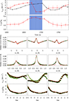 |
Fig. 7. Same as Fig. 6, but for a downflowing umbral flash profile. |
| In the text | |
|
Fig. 8. Same as Fig. 6, but for point B in Fig. 2, where standing waves are found in the low chromosphere. |
| In the text | |
|
Fig. 9. Same as Fig. 6, but for point C in Fig. 2, where standing waves are found in the low chromosphere. |
| In the text | |
|
Fig. 10. Same as Fig. 6, but for point D in Fig. 2, where standing waves are found in the low chromosphere. |
| In the text | |
Current usage metrics show cumulative count of Article Views (full-text article views including HTML views, PDF and ePub downloads, according to the available data) and Abstracts Views on Vision4Press platform.
Data correspond to usage on the plateform after 2015. The current usage metrics is available 48-96 hours after online publication and is updated daily on week days.
Initial download of the metrics may take a while.